Optimal Bidding of a Microgrid Based on Probabilistic Analysis of Island Operation

Abstract

Island operation of a microgrid increases operation survivability and reliability when there is a large accident in a main grid. However, because a microgrid typically has limited generation capability, a microgrid operator (MGO) has to take the risk of island operation into account in its market participation and generation scheduling to ensure efficient operation. In this paper, a microgrid islanding event is interpreted as a trade suspension of a contract, and a set of islanding rules is presented in the form of a market rule. The risk of island operation is evaluated by modeling the microgrid islanding stochastically using an islanding probability function, which is defined in the form of a conditional probability to reflect the influence of outside conditions. An optimal bidding strategy is obtained for the MGO by formulating and solving an optimization problem to minimize the expected operating cost. The effectiveness of the proposed method was investigated by numerical simulations in which the proposed method and two other methods were applied to the same microgrid. Numerical sensitivity analyses of the coefficients of the islanding probability function were conducted to determine how an MGO copes with changes in outside conditions.

1. Introduction

Microgrids are entities in medium- and low-voltage distribution networks that consist of small subsystems such as generators, loads, and energy storage systems. An entity called a microgrid operator (MGO) controls these distributed resources and makes decisions in the electricity market [1,2,3]. Normally, an MGO tries to maintain its connection to the main grid to obtain economic benefits from the market and to utilize ancillary services such as frequency control that are provided by the independent system operator (ISO). However, if a large accident occurs in the main grid, an MGO could cut its connection to the main grid and operate in islanded mode to protect its systems [4,5]. During island operation, the MGO must meet the demand by itself while simultaneously maintaining the system reliability. Because island operation of a microgrid is quite distinct from traditional power system operation, many studies on microgrid islanding have been conducted.

Microgrid stability analysis during the islanding process has been studied previously [6,7,8], in which the system modeling and control strategy of a microgrid was investigated. In [9,10], various control schemes for distributed generators were studied to determine how best to synchronize the frequency and voltage of an islanded microgrid with that of the main grid during the reconnection process. Generation scheduling of a microgrid in the case of an unexpected islanding event has also been studied [11,12,13].

In many previous studies [4,5,6,7,8,9,10,11,12,13], it was commonly assumed that microgrid islanding is a protective action that is intentionally taken by an individual MGO to ensure the reliability of its electricity supply. In contrast, [14] proposed a different perspective on microgrid island operation, which can be treated as load shedding by the ISO undertaken to ensure that the system operates stably. From this perspective, microgrids are viewed as a type of distribution network that can be isolated from the main grid by the ISO if they affect the system stability adversely. Microgrid islanding is thus associated with the system reserve operation in [14], and a probabilistic analysis approach was proposed that enables the MGO to consider uncertain islanding at the operational level; e.g., unit commitment and economic dispatch. However, the approach proposed in [14] has a practical limitation in that microgrid islanding only occurs according to a simple rule in the market: “A breach of contract unconditionally triggers an islanding event”.

The research work described in this paper was an extension of [14] and focused on realistic triggering situations for microgrid islanding in terms of not only a market contract but also grid conditions. Various causes of microgrid islanding were translated and added to the set of islanding rules presented in [14]. Given the inherent unpredictability of grid conditions, microgrid islanding events were modeled as stochastic events, and a probabilistic analysis was conducted using a conditional probability function to evaluate the islanding risk. An MGO’s risk hedging strategy for minimizing the expected daily operating cost of a microgrid was then formulated as an optimization problem, to determine the optimal amount of reserve band bid.

The remainder of this paper is organized as follows. In Section 2, a brief review of [14] is presented. Section 3 introduces a new set of microgrid islanding rules in the form of market rules. The results of a probabilistic and quantitative analysis of microgrid islanding risks are presented in Section 4. The results of an investigation of an MGO’s operation strategy based on these analysis results and conducted using numerical simulations are presented in Section 5. Finally, a discussion of the results and conclusions are presented in Section 6.

2. Microgrid Islanding Limited to Market Operation

Market participants, such as wind generators, whose generation output is difficult to forecast have recently increased in number. This increased uncertainty burdens an ISO with reserve operations more so than in the past [15,16,17]. Several electricity markets have attempted to impose penalty costs on participants when their actual consumption/generation was outside a specified range around the energy bid [18,19,20,21]. For example, in [21], a participant whose actual consumption/generation was outside the range of 95%–105% of its energy bid received a price penalty of 25%. Ilic et al. [22] proposed a new market structure, called a power-exchange-for-frequency-control (PXFC) market, to describe this type of system. In a PXFC market, each participant is expected to submit both an energy bid and a reserve band bid, and the latter is the criterion for imposing a penalty cost on its large uncertainty. In other words, the PXFC structure is postulated on the existence of smart and active market participants who can take on some role in the system reserve operation. Therefore, a PXFC market is regarded as a suitable market environment for microgrid operation and is used to describe the reserve market in [14].

In addition, reference [14] proposed a microgrid islanding rule in the form of a PXFC market rule, and microgrid islanding was regarded as another type of penalty that the market imposes on large uncertainty. Under this assumption, an MGO must accept its island operation when it breaches the reserve band bid. To evaluate the penalty associated with microgrid islanding, microgrid islanding was modeled as a binomial event between two states in [14]: grid-connected and islanded states. The probability of triggering an islanding event, $p_{ij}$, is determined by the purchased reserve band and the microgrid uncertainty model as follows:

$$p_{ij}={\displaystyle {\int }_{-\infty }^{-B{D}_i}{f}_{{\Delta }_{ij}}\cdot d{\Delta }_{ij}}+{\displaystyle {\int }_{B{D}_i}^{\infty }{f}_{{\Delta }_{ij}}\cdot d{\Delta }_{ij}}.$$

(1)

Because the probability in Equation (1) depends on the reserve band bid, an MGO can minimize its operating cost by strategically purchasing the band from the market, as expressed below:

$$\underset{BD}{\min }{C}_{\mathrm{TOT}}$$

(2)

According to [14], the microgrid islanding risk can be analyzed by defining a new index microgrid islanding probability (MIP), or $k$, which reflects the probability of being in the islanded state during a given period of time. Utilizing MIP, $C_{\mathrm{TOT}}$ can be represented in the form of a probabilistic linear combination of $CG$ and $CI$ as follows:

$$\begin{array}{cc}\hfill C_{\mathrm{TOT}}& ={(1-k(BD))}^T\cdot CG(BD)+k^T(BD)\cdot CI\hfill \\ & ={\displaystyle \sum _{i=1}^{N_{stg}}\left[\left\{1-k_i(BD)\right\}\cdot C{G}_i(B{D}_i)+k_i(BD)\cdot C{I}_i\right]}\hfill \end{array}$$

(3)

The MIP $k$ given by Equation (3) enables MGOs to evaluate the risk of an islanding event at the operation or planning level.

3. New Microgrid Islanding Rules, Including the Grid Condition

Unplanned islanding will interrupt the electricity trade of a microgrid, if the microgrid participates in an electricity market and makes a contract. In this situation, a market rule about the contract breach caused by microgrid islanding is necessary for protecting the rights and interests of market participants. In order to enact a market rule about microgrid islanding, the cause and responsibility for the occurrence of islanding should be initially analyzed. To this end, the observance of a market contract was selected as a criterion of an islanding occurrence in [14]. However, this method may too often trigger the island operation of microgrids, thereby possibly rendering the system operation unstable or inefficient. Furthermore, the market rule in [14] is incomplete in terms of describing the whole microgrid operation. This is because it does not include the islanding events as a protective action, which is a prime reason for utilizing the microgrid technology. Considering the above points, microgrid islanding rules must consider the operating condition of the grid as well as the market contract for real-world practical application. The following new set of microgrid islanding rules was proposed in this study.

• Rule I: The ISO can disconnect any microgrid whose actual consumption/generation is outside the contracted reserve band from the energy bid, if it is necessary to do so for system frequency regulation.
• Rule II: If an MGO violates its reserve band contract but does not get disconnected, it must pay a penalty for the violation.
• Rule III: If a disturbance occurs in the grid, an ISO/MGO can impose/adopt island operation as a protective action.
• Rule IV: If islanding occurs during a given step of a stage, it lasts for the duration of the remaining steps of that stage, as well as the next stage, after which the microgrid attempts to reconnect to the main grid.
• Rule V: A reconnection attempt by an islanded microgrid can fail. In the case of failure, the MGO can attempt to reconnect again during the next stage.
• Rule VI: When either an ISO or MGO make a decision concerning islanding, both entities individually cover the loss from trade suspension due to the islanding.

In Rule VI and V, the step and the stage represent time units for the imbalance settlement/islanding occurrence and the contract in the PXFC market, respectively. For example, if a contract in the energy market is on an hourly basis and the imbalance settlement is carried out every 15 min, a day consists of 24 stages and each stage consists of 4 steps.

According to Rule I, an islanding event may or may not occur even if an MGO violates its reserve band contract. In other words, Rule I shows that an MGO’s breach of the band contract is a soft condition of the occurrence of an islanding event, whereas it was a hard condition in [14]. This is much more realistic, considering that the effect on the system operation from an imbalance generated by a microgrid varies with the system status. For example, assume that the ISO imposes an island operation on a microgrid that violates the band contract when the system frequency is stable. In this case, the islanding event could be an unintentional disturbance caused by the ISO itself and could adversely affect the system stability. The ISO thus must consider not only the contract observance of a particular microgrid, but also the condition of the entire system for operating the system stably and reliably. However, if Rule I existed alone, some optimistic or selfish MGOs could purchase smaller reserve bands from the market than the imbalances that they actually generate. To address this problem, Rule II was created to impose a penalty cost on an MGO that violates the contract but is still connected to the main grid. Therefore, an MGO must purchase its reserve band capacity from the market, taking into consideration the risks of both island operation and penalty payments. Rule III represents another type of microgrid islanding caused by disturbance in the system. This islanding action can be taken by an MGO or ISO to protect the reliability of its operation [4,5], and this can occur at any time, regardless of the contract violation. Many accidents, such as an overflow due to a line fault in the network or a shortage of the system reserve due to a sudden demand increase, can trigger these types of microgrid islanding.

Rule IV specifies the minimum duration of an island operation in the same manner as in [14]. The minimum duration can be determined by market regulation and physical constraints [23,24]. During this time period, the MGO controls the frequency and voltage in the microgrid and prepares for reconnection to the main grid. This reconnection could end in failure without sufficient synchronization [9,10]. Because a reconnection failure affects the duration of the island operation, synchronization and reconnection of the microgrid need to be considered in evaluating the risk of islanding and in subsequently calculating the expected operating cost. Thus, the possibility of reconnection failure is specified in Rule V. Rule VI prescribes the responsibility between the MGO and ISO concerning trade suspension of electricity as a result of islanding. This type of responsibility rule, which defines the indemnification for a breach of the contract, is necessary for all types of future trading and varies from one contract to another [25,26,27]. Therefore, this paper proposes Rule VI as a simple example of an indemnification rule that requires that the ISO and MGOs handle their respective losses due to islanding.

4. Optimal Operation Strategy by MGO

4.1. Defining the Cost Functions

Prior to establishing its operation strategy, an MGO has to define its operating cost functions. The MGO’s operating cost in grid-connected mode can be defined as shown below:

$$C{G}_i=R{G}_i\left(B{D}_i\right)+E{G}_i$$

(4)

The reserve supply cost term $R{G}_i$ consists of the band purchase cost and the imbalance penalty cost imposed according to Rule II; i.e.,

$$R{G}_i={\lambda }_i^{BD}\cdot B{D}_i+{\displaystyle \sum _{j}P{G}_{ij}}$$

(5)

The imbalance penalty cost $P{G}_{ij}$ is determined according to a prearranged mutual agreement among the market participants. The penalty cost function was defined in this study as the product of the penalty price and the band violation capacity, as shown below [21].

$$P{G}_{ij}=\{\begin{array}{cc}{\lambda }_i^{PG}\cdot \left|{\Delta }_{ij}-B{D}_i\right|& \mathrm{if}\left|{\Delta }_{ij}\right|>B{D}_i\\ 0& \mathrm{otherwise}\end{array}$$

(6)

Similarly, an MGO’s operating cost in the islanded mode is expressed as follows:

$$C{I}_i=R{I}_i+E{I}_i$$

(7)

The reconnection cost $R{I}_i$ represents the total cost that the MGO has to pay during the island operation, except for the energy supply costs, which consist of the control cost for stabilization and reconnection, the wear cost associated with switching, etc. The values of the energy supply cost terms $E{G}_i$ and $E{I}_i$ in Equations (4) and (7) are determined using a procedure similar to the economic dispatch. An MGO can also arrive at its energy bidding ($P_i^{\mathrm{ext}}$) and generation schedule ($P_i^{G,\mathrm{int}}$ and $P_i^{I,\mathrm{int}}$) by solving the following sub-optimization problems:

$$E{G}_i=\underset{(P_i^{G,\mathrm{int}},P_i^{\mathrm{ext}})}{\min }\left[G_i(P_i^{G,\mathrm{int}})+M_i(P_i^{\mathrm{ext}})\right]$$

(8)

$$E{I}_i=\underset{(P_i^{I,\mathrm{int}},P_i^{LS})}{\min }\left[G_i(P_i^{I,\mathrm{int}})+L{S}_i(P_i^{LS})\right]$$

(9)

where the sum of $P_i^{G,\mathrm{int}}$ and $P_i^{\mathrm{ext}}$, as well as the sum of $P_i^{I,\mathrm{int}}$ and $P_i^{LS}$, should be equal to the forecasted demand for the microgrid, $D_i$. Assuming that load shedding does not occur in the grid-connected mode (i.e., assuming that the price of load shedding is much higher than the price of other generation resources), the load shedding cost term $L{S}_i$ is not considered in Equation (8).

4.2. Microgrid Islanding Model

Islanding Rules I and III in Section 3 generalize the triggering conditions for microgrid islanding. Because this generalized island operation can be affected by both the reserve band contract and the system condition, the triggering condition expressed by Equation (1) is not sufficient in this case. To resolve this problem, a conditional probability function, $g_{ij}$, which represents the islanding occurrence probability according to ${\Delta }_{ij}$, was newly defined in this study. An MGO can formulate the triggering condition using this conditional probability function, expressed as shown below:

$$p_{ij}={\displaystyle {\int }_{-\infty }^{\infty }\left\{g_{ij}\left({\Delta }_{ij},B{D}_i\right)\cdot f_{{\Delta }_{ij}}\left({\Delta }_{ij}\right)\right\}d{\Delta }_{ij}}$$

(10)

$$g_{ij}=\mathrm{Pr}\left(A|{\Delta }_{ij}\right)$$

(11)

where A in Equation (11) is a set of islanding events; $g_{ij}$ is a function of ${\Delta }_{ij}$ and $B{D}_i$, which are the basic variables of reserve operation in the PXFC market environment; and $g_{ij}$ reflects the system conditions that can affect microgrid islanding, which may be various types of functions, depending on the grid condition. In general, the value of $g_{ij}$ is close to zero when ${\Delta }_{ij}$ is smaller than or similar to $B{D}_i$, and it increases as ${\Delta }_{ij}$ increases. The following sigmoid-type function is an example of $g_{ij}$:

$$g_{ij}=\mathrm{C}+(1-\mathrm{C})\cdot {\left[1+e^{-\mathrm{a}\cdot (\left|{\Delta }_{ij}\right|-\mathrm{b}\cdot B{D}_i)}\right]}^{-1}$$

(12)

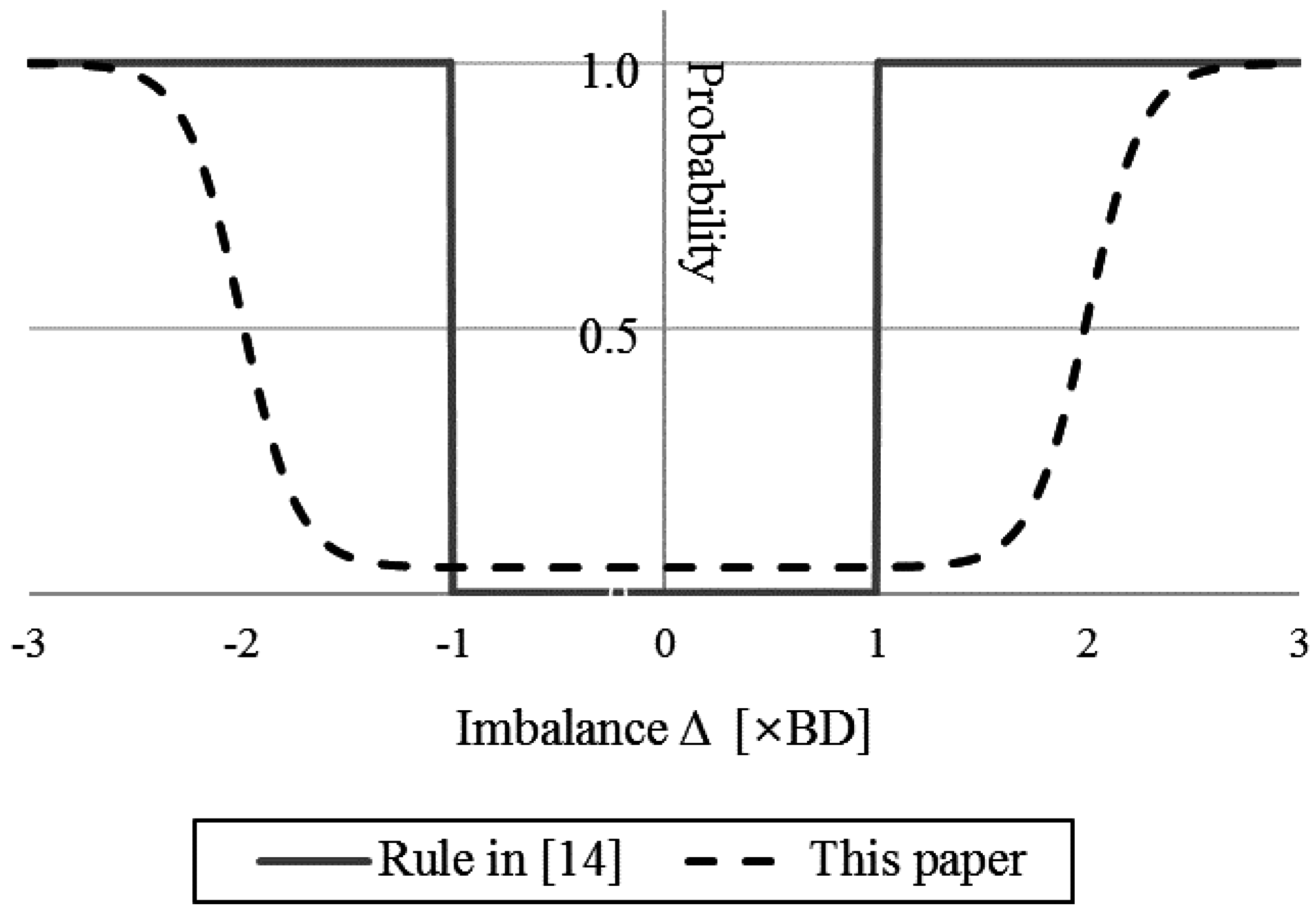
where $\mathrm{a}$, $\mathrm{b}$, and $\mathrm{C}$ are constant coefficients and can represent the grid condition. For example, two coefficients $\mathrm{a}$ and $\mathrm{b}$ may indirectly reflect the remains of spinning reserve or ISO’s load shedding operation scheme, and $\mathrm{C}$ can represent the line fault probability. The dashed line in Figure 1 is an example of Equation (12). This figure shows that an islanding event occurs stochastically even if an MGO violates its reserve band contract, and the occurrence probability increases as the imbalance generated by the MGO increases. A comparison of Equations (1) and (10) shows that the shape of the conditional probability function $g_{ij}$ in Equation (1) can be derived as the solid line in Figure 1. This quantum-well-shaped probability function is consistent with the fact that, according to [14], an islanding event occurs unconditionally when an MGO violates its reserve band contract.

The microgrid islanding model of Equation (10) with the conditional probability function clarifies the triggering condition for an islanding event and plays a key role in quantitative analysis of the calculated MIP. In other words, proper modeling of $g_{ij}$ is essential to evaluate the risk of island operation. However, the main subject of this paper is to present an optimal operation strategy for a microgrid, taking into consideration the stochastic island operation. Therefore, it is assumed that the islanding model $g_{ij}$ is given to the MGO as the demand uncertainty model $f_{{\Delta }_{ij}}$ is given.

4.3. Formulating the Objective Function and MIP

The MIP value of the ith stage, $k_i$, is the ratio of the expected number of steps in which the islanded state is maintained in the ith stage to the total number of steps in that stage. The expression of $k_i$ can be derived by examining the form of the expected incurred cost during the ith stage. To obtain this form, two cases are considered at the beginning of the ith stage: $X_{i,0+}=0$ (grid-connected) and $X_{i,0+}=1$ (islanded).

For the grid-connected mode ($X_{i,0+}=0$), the state may persist until the end of the ith stage with no islanding event (Case G1), or the state may transfer during the stage with an islanding event (Case G2). The expected cost of Case G1 can be calculated as follows:

$$C_i^{\mathrm{G}1}={\displaystyle {\int }_{{\overline{\Delta }}_i}C{G}_i\cdot {\displaystyle \prod _{j=1}^{N_{stp}}\left(1-g_{ij}\right)}\cdot f_{{\overline{\Delta }}_i}\cdot d{\overline{\Delta }}_i}$$

(13)

The pi-product of $1-g_{ij}$ in the integration indicates that no islanding event is triggered during the stage. $C{G}_i$ corresponds to the operating cost in that case. For Case G2, if an islanding event occurs during the jth step of the ith stage, the expected cost can be calculated as follows:

$$C_{ij}^{\mathrm{G}2}={\displaystyle {\int }_{{\overline{\Delta }}_{ij}}\left(C{G}_{ij}+C{I}_{ij}\right)\cdot \left\{{\displaystyle \prod _{m=1}^{j-1}\left(1-g_{ij}\right)}\cdot g_{ij}\right\}\cdot f_{{\overline{\Delta }}_{ij}}\cdot d{\overline{\Delta }}_{ij}}$$

(14)

The sum $C{G}_{ij}+C{I}_{ij}$ corresponds to the incurred cost during the stage, and its components can be calculated as follows.

$$C{G}_{ij}=\left(\frac{j-1}{N_{stp}}\right)\cdot \left(E{G}_i+{\lambda }_i^{BD}\cdot B{D}_i\right)+{\displaystyle \sum _{k=1}^{j-1}P{G}_{ik}}$$

(15)

$$C{I}_{ij}=\left(\frac{N_{stp}-j+1}{N_{stp}}\right)\cdot \left(C{I}_i\right)$$

(16)

where $C{G}_{ij}$ is the operating cost before the islanding event occurs, and $C{I}_{ij}$ is the operating cost after the islanding event occurs. The pi-product in Equation (14) represents the event-triggering probability of Case G2. Because an islanding event may occur during any step in the ith stage, the total expected cost of Case G2 can be represented as the summation of Equation (14):

$$C_i^{\mathrm{G}2}={\displaystyle \sum _{j=1}^{N_{stp}}{C}_{ij}^{\mathrm{G}2}}$$

(17)

For the islanded mode ($X_{i,0+}=1$), the calculation of the expected cost must reflect the situation in which the islanded microgrid attempts to synchronize and reconnect with the main grid during the ith stage. Because this trial results in success or failure (Case I1/I2), the expected values of the operating costs for these two cases are represented as follows:

$$C_i^{\mathrm{I}1}=C{I}_i\cdot {\alpha }_i$$

(18)

$$C_i^{\mathrm{I}2}=C{I}_i\cdot \left(1-{\alpha }_i\right)$$

(19)

where ${\alpha }_i$ in Equations (18) and (19) indicates the success probability of reconnection in the ith stage. As mentioned in Section 3, this probability depends on the grid condition and the synchronization capability of the MGO. Assuming that the synchronization error is a function of the time that is used for synchronizing, ${\alpha }_i$ can be represented as shown below:

$${\alpha }_i=J\left(i-s\right)$$

(20)

where index i and s represent the reconnection attempt stage and the islanding trigger stage, respectively. The value of ${\alpha }_i$ will be different, even if two identical microgrids tried to reconnect to the main grid at the same time, if the duration of island operation was different for the two microgrids. For example, if the success probability is inversely proportional to the synchronization time, or $i-s$, the following can serve as a possible reconnection attempt model.

$${\alpha }_i=J\left(i-s\right)=\{\begin{array}{ll}0.6& \mathrm{if}i-s=1\\ 0.8& \mathrm{if}i-s=2\\ 1.0& \mathrm{if}i-s\ge 3=N_{\alpha }\end{array}$$

(21)

The number in the probability step, $N_{\alpha }$, which has a value of 3 in Equation (21), can also be a part of this reconnection model. This means that this MGO is able to recover its grid connection in less than $N_{\alpha }$ stages.

Consequently, the expected value of the overall operating cost for all stages is given by the following:

$$C_{TOT}={\displaystyle \sum _{i=1}^{N_{stg}}[\left\{\mathrm{Pr}\left(X_{i,0+}=0\right)\cdot \left(C_i^{\mathrm{G}1}+C_i^{\mathrm{G}2}\right)\right\}}+\left\{\mathrm{Pr}\left(X_{i,0+}=1\right)\cdot \left(C_i^{\mathrm{I}1}+C_i^{\mathrm{I}2}\right)\right\}]$$

(22)

The MIP formulation can be derived by comparing Equation (22) to Equation (3). After substituting Equations (13) and (17)–(19) into each $C_i^X$ in Equation (22), and after some arrangement, MIP $k_i$ can be expressed as follows:

$$k_i=\mathrm{Pr}(X_{i,0+}=0)\times {\displaystyle \sum _{j=1}^{N_{stp}}\left[\left(\frac{N_{stp}-j+1}{N_{stp}}\right)\cdot P_{\mathrm{no}\_\mathrm{event}}^{i,j}\right]}+\mathrm{Pr}(X_{i,0+}=1)\times 1$$

(23)

$$P_{\mathrm{no}\_\mathrm{event}}^{i,j}={\displaystyle {\int }_{{\overline{\Delta }}_i}{\displaystyle \prod _{m=1}^j\left\{1-g_{im}\right\}}\cdot f_{{\overline{\Delta }}_i}\cdot d{\overline{\Delta }}_i}$$

(24)

According to Rules III and IV, $\mathrm{Pr}(X_{i,0+}=0)$ and $\mathrm{Pr}(X_{i,0+}=1)$ in Equation (23) can be represented by the following recurrence equation:

$$\begin{array}{ccc}\hfill \mathrm{Pr}\left(X_{i,0+}=0\right)& =& \left[\mathrm{Pr}\left(X_{i-1,0+}=0\right)\cdot P_{\mathrm{no}\_\mathrm{event}}^{i-1,N_{stp}}\right]\hfill \\ & & +{\displaystyle \sum _{k=1}^{N_{\alpha }}\left[\mathrm{Pr}\left(X_{i-(k+1),0+}=0\right)\cdot P_{\mathrm{event}}^{i-(k+1)}\cdot \left\{{\displaystyle \prod _{l=2}^k\left(1-{\alpha }_{i-l}\right)\cdot {\alpha }_{i-1}}\right\}\right]}\hfill \end{array}$$

(25)

$$P_{\mathrm{event}}^{i-(k+1)}=\left\{1-{\displaystyle {\int }_{{\overline{\Delta }}_{i-(k+1)}}{\displaystyle \prod _{j=1}^{N_{stp}}\left\{1-g_{i-(k+1),j}\right\}}\cdot f_{{\overline{\Delta }}_{i-(k+1)}}\cdot d{\overline{\Delta }}_{i-(k+1)}}\right\}$$

(26)

The first term on the right-hand side of Equation (25) represents the situation in which there is no islanding event during the (i − 1)th stage, as in Equation (13), and $X_{i-1,0+}=0$ is maintained until the beginning of the ith stage. The second term represents all of the situations in which the MGO recovers from the islanded state during the (i − 1)th stage and can start the ith stage in a grid-connected state. The summation in the second term indicates that a microgrid starts in the grid-connected state at the beginning of the (i – k + 1)th stage. This microgrid enters the islanded state during this stage and recovers its grid connection after k reconnection attempts.

5. Numerical Simulations

5.1. Simulation Settings

In the simulations, a day consisted of 24 stages, and each stage consisted of four steps. In other words, a contract in the energy market is on an hourly basis, and the imbalance settlement and islanding occurrence is carried out every 15-min. The cost functions of the microgrid in Equations (4)–(9) were formulated by taking the values given in [14] as follows:

$$G_i(P_i^{\mathrm{int}})=48.425\cdot P_i^{\mathrm{int}} \mathrm{for} 10\le P_i^{\mathrm{int}}\le 40$$

(27)

$$M_i(P_i^{\mathrm{ext}})={\lambda }_i^E\cdot P_i^{\mathrm{ext}} \mathrm{for} 10\le P_i^{\mathrm{ext}}\le 50$$

(28)

$$R{G}_i(B{D}_i)={\lambda }_i^{BD}\cdot B{D}_i+{\displaystyle \sum _{j}P{G}_{ij}}\left({\lambda }_i^{PG}\right)$$

(29)

$$L{S}_i(P_i^{LS})=3000\cdot P_i^{LS} \mathrm{for} 0\le P_i^{LS}\le P_i^{\mathrm{int}}+P_i^{\mathrm{ext}}$$

(30)

$$R{I}_i=30$$

(31)

where $P_i^{\mathrm{int}}$ represents either $P_i^{G,\mathrm{int}}$ or $P_i^{I,\mathrm{int}}$, depending on the corresponding operating mode, and ${\lambda }_i^E$ and ${\lambda }_i^{BD}$ are the hourly prices of the energy and reserve band market, respectively. It was assumed that ${\lambda }_i^E$ and ${\lambda }_i^{BD}$ have the same value and that the MGO is a price taker. These assumptions were made to exclude complex market phenomena, e.g., gaming in joint energy and reserve markets [28], and to focus on the MGO’s reserve bidding strategy with respect to the islanding risk. Day-ahead locational marginal prices from Pennsylvania–New Jersey–Maryland Interconnection LLC (PJM) on 20 August 2015 [29] were used for ${\lambda }_i^E$ and ${\lambda }_i^{BD}$. The penalty cost function given by Equation (6) was utilized and the penalty price ${\lambda }_i^{PG}$ was set to 125% of ${\lambda }_i^E$. The forecasted demand of the microgrid was determined based on the day-ahead market demand from PJM on the same day and scaled with a maximum of 50 MW. A normal Gaussian distribution with a mean of zero and a variance of ${\sigma }_{ij}$ was used as the uncertainty model of the demand in Equation (10). The standard deviation ${\sigma }_{ij}$ was randomly selected in the range of 5%–20% of the forecasted demand. The sigmoid-shaped function in Equation (12) was used for the microgrid islanding model. The coefficients in Equation (12) were determined to result in an islanding probability of 50% when each MGO violates the band contract by twice as much as the contracted capacity, expressed as follows:

$$g_{ij}=0.01+0.99\cdot {\left[1+e^{-10\cdot (\left|{\Delta }_{ij}\right|-2\cdot B{D}_i)}\right]}^{-1}$$

(32)

For the reconnection model, the probability step function in Equation (21) with $N_{\alpha }=3$ was assumed. To assess the effectiveness of the proposed method, three reserve bidding methods were studied and compared: Method I, in which the reserve band is 20% of the demand in each stage; Method II, proposed in [14]; and Method III, proposed in this paper. The values for all of the market and grid conditions are given in

Table 1. Simulation parameters.

Stage	1	2	3	4	5	6
Forecasted demand [MW]	35.68	33.59	32.50	31.70	32.00	33.31
Standard deviation [MW]	3.61	4.63	2.72	5.16	2.82	4.19
Market price [$/MWh]	22.99	21.80	19.52	18.23	18.49	21.60
Stage	7	8	9	10	11	12
Forecasted demand [MW]	36.09	38.71	41.03	43.10	45.40	47.00
Standard deviation [MW]	5.59	7.11	7.95	5.69	3.21	3.40
Market price [$/MWh]	23.48	24.23	25.60	27.89	31.79	32.16
Stage	13	14	15	16	17	18
Forecasted demand [MW]	48.33	49.31	49.57	49.90	50.00	49.48
Standard deviation [MW]	4.28	8.68	4.37	8.59	4.33	9.37
Market price [$/MWh]	33.16	36.15	37.57	37.75	36.37	34.63
Stage	19	20	21	22	23	24
Forecasted demand [MW]	47.78	46.29	46.23	44.83	40.63	37.15
Standard deviation [MW]	4.90	3.68	4.05	6.38	4.92	3.82
Market price [$/MWh]	31.85	30.73	31.16	28.36	24.42	23.69

. All the simulations were performed with MATLAB R2016a (Mathworks, Natick, MA, USA, and the optimization problems were solved by the pattern search algorithm [30].

5.2. Simulation Results: Cost Analysis

The simulated daily operating cost of each case is shown below, and the corresponding reserve band capacity and calculated MIP for each stage are listed in

Table 2. Optimal band capacity and MIP values for the three cases.

Stage		1	2	3	4	5	6
Band_Capacity [MW]	Method I	7.136	6.718	6.500	6.340	6.400	6.662
	Method II	8.468	11.497	7.157	11.015	7.522	11.315
	Method III	5.381	6.781	4.280	7.630	4.412	6.131
MIP [N/A]	Method I	0.025	0.072	0.090	0.115	0.128	0.099
	Method II	0.025	0.063	0.077	0.079	0.079	0.079
	Method III	0.032	0.082	0.097	0.097	0.096	0.097
Stage		7	8	9	10	11	12
Band Capacity [MW]	Method I	7.218	7.742	8.206	8.620	9.080	9.400
	Method II	11.625	21.218	25.610	20.891	12.376	11.942
	Method III	8.541	11.915	14.145	10.726	6.367	6.784
MIP [N/A]	Method I	0.108	0.177	0.263	0.235	0.132	0.086
	Method II	0.079	0.079	0.079	0.078	0.078	0.078
	Method III	0.098	0.093	0.085	0.081	0.080	0.079
Stage		13	14	15	16	17	18
Band Capacity [MW]	Method I	9.666	9.862	9.914	9.980	10.000	9.896
	Method II	16.479	30.497	15.535	28.224	16.400	31.827
	Method III	8.449	16.283	8.582	16.106	8.493	17.325
MIP [N/A]	Method I	0.077	0.130	0.158	0.151	0.150	0.177
	Method II	0.078	0.078	0.078	0.078	0.078	0.078
	Method III	0.079	0.079	0.079	0.079	0.079	0.080
Stage		19	20	21	22	23	24
Band Capacity [MW]	Method I	9.556	9.258	9.246	8.966	8.126	7.430
	Method II	17.528	14.186	15.089	22.687	12.726	7.660
	Method III	9.427	7.177	7.700	11.080	7.555	4.914
MIP [N/A]	Method I	0.196	0.119	0.084	0.089	0.098	0.088
	Method II	0.078	0.078	0.078	0.078	0.078	0.079
	Method III	0.080	0.079	0.079	0.080	0.085	0.109

.

• Method I: $81,511
• Method II: $68,950
• Method III: $64,582

The operating cost for the proposed method (Method III) is 20.77% less than that of Method I and 6.34% less than that of Method II. In Method I, the MGO prepared a reserve band proportional to its demand using a constant ratio and did not consider any other market or grid conditions. Therefore, the prepared reserve band is inefficient when the occurrence of an expensive islanding event is dependent on the market and grid conditions. In other words, the MGO sometimes pays too much in hedging the risk of island operation, and sometimes the MGO takes too much risk of island operation. In contrast, with Methods II and III, the MGO predicts the island operation based on the uncertainty modeling and determines the reserve band based on the market condition. Therefore, these two methods yield relatively small MIP values for the MGO and better performance, in terms of operating cost, than Method I.

However, as mentioned in Section IV, there is a large difference between Methods II and III in terms of the islanding model. Method III models microgrid islanding as a stochastic event that is dependent on the grid conditions, whereas Method II models it with a simple rule in the market. Given that the imbalance generated by a microgrid generally does not have a large effect on the main grid when the system is stable, Method II tends to overstate the risk of island operation. As a result, the operating costs associated with Method III are smaller than the operating costs associated with Method II, and the MIP values during 24 stages by Method III are always larger with Method III than with Method II. Specifically, Method III reduces the band purchase cost by $5,206 compared to Method II, while the larger MIP values of Method III only increase the expected islanded operating cost by $214 compared to Method II.

5.3. Simulation Results: Sensitivity Analysis

To investigate the effect of the grid condition on the MGO’s reserve bidding strategy, the simulation results were examined by varying the values of two of the coefficients, $\mathrm{b}$ and $\mathrm{C}$, in Equation (12), as well as the penalty price ${\lambda }_i^{PG}$. The results of these simulations provide indirect insight into how an MGO can cope with changes in the system operating conditions, such as the ISO’s frequency regulation policy ($\mathrm{b}$ and ${\lambda }_i^{PG}$) and the probability of a line fault that trips the circuit breaker between the microgrid and the main grid ($\mathrm{C}$). To clarify the relationship between the MGO’s reserve bidding and each parameter, the following simulations were performed only for the 1st stage in Table 1.

The coefficient $\mathrm{b}$, which is related to the increasing speed of islanding probability when the amount of the MGO’s contract violation increases, was varied from 1.5 (fast increase) to 10 (slow increase). The other coefficients $\mathrm{a}$ and $\mathrm{C}$ were fixed as in Equation (29), and the penalty price was fixed at 125% of ${\lambda }_i^E$.

Table 3. Optimal reserve band capacities, MIPs, and operating costs according to islanding policy changes.

b	1.5	2.0	5.0	10.0
$B{D}^{*}$ [MW]	5.932	4.691	2.226	1.406
MIP [N/A]	0.058	0.047	0.030	0.025
$C_{\mathrm{TOT}}$ [$]	1244	1211	1151	1140
$k_1\cdot C{I}_1$ [$]	103	85	53	45
$\left(1-k_1\right)\cdot C{G}_1$ [$]	1141	1126	1098	1095

shows the optimal reserve band capacities and corresponding MIPs and operating costs. The results show that MGO’s reserve bidding is highly sensitive to the change of $\mathrm{b}$. Specifically, the MGO decreases the purchase amount of the reserve band as the value of $\mathrm{b}$ increases. The reason for this is that an increase in $\mathrm{b}$ enables the MGO to have the same occurrence probability of an islanding event with the reduced reserve band. For example, the expected value of the islanded operating cost decreases by 47.1% when $\mathrm{b}$ changes from 2 to 10, as shown in Table 3, even though the MGO decreases the amount of band purchase by 70%.

On the other hand, the MGO’s reserve bidding is conditionally sensitive to changes in ${\lambda }_i^{PG}$. As

Table 4. Optimal reserve band capacities according to penalty price and islanding policy changes.

${\mathit{\lambda }}_{\mathit{i}}^{\mathit{P}\mathit{G}}$[$\times {\mathit{\lambda }}_{\mathit{i}}^{\mathit{E}}$]		1.00	1.25	1.50	2.00
$\mathbf{b}$	1.5	5.932	5.932	5.932	5.932
	2.0	4.690	4.691	4.692	4.693
	5.0	2.207	2.226	2.246	2.286
	10.0	1.321	1.406	1.516	1.745

shows, the amount of reserve band purchased by the MGO is proportional to the value of ${\lambda }_i^{PG}$, especially when $\mathrm{b}$ has a large value. This is related to the proportion of the imbalance penalty cost to the total operating cost. In other words, if the value of $\mathrm{b}$ is large, the MGO can easily hedge the islanding risk and maintain its grid connection with a smaller reserve band, but it will have to pay a considerable penalty cost for the band contract violation. Therefore, the influence of the imbalance penalty cost on the MGO’s reserve bidding strategy is larger in this case. In contrast, because a small value of $\mathrm{b}$ compels the MGO to prepare a large reserve band, the chance that the MGO violates its band contract decreases.

Next, the value of the coefficient $\mathrm{C}$ was varied from 0 to 0.5.

Table 5. Optimal reserve band capacities, MIPs, and operating costs according to fault probability changes.

C	0	0.01	0.05	0.10	0.50
$B{D}^{*}$ [MW]	4.695	4.691	4.679	4.661	4.464
MIP [N/A]	0.023	0.047	0.139	0.244	0.771
$C_{\mathrm{TOT}}$ [$]	1196	1211	1267	1330	1648
$k_1\cdot C{I}_1$ [$]	41	85	249	436	1378
$\left(1-k_1\right)\cdot C{G}_1$ [$]	1155	1126	1018	894	270

shows the specific values of $\mathrm{C}$ and the corresponding results for the optimal reserve band capacity, MIP, and operating cost. As Table 5 shows, the MGO slightly decreases the purchase amount of the reserve band as $\mathrm{C}$ increases. This reserve bidding strategy may seem to be irrational because a large $\mathrm{C}$ increases the values of MIP and $C_{\mathrm{TOT}}$. However, this is a reasonable decision, considering that an islanding event caused by $\mathrm{C}$ is irrelevant to the amount of the MGO’s band contract, according to Rule III. In other words, the MGO increasingly regards islanding as an inevitable event as $\mathrm{C}$ increases because the portion of islanding risk that the MGO can manage with its reserve band decreases. In the extreme case, the optimal reserve band capacity is 0 when $\mathrm{C}=1$. However, it has been verified that the influence of $\mathrm{C}$ on an MGO’s operation strategy is negligible in the region of realistic values (approximately 1%) [31].

6. Conclusions

We have described a method for analyzing the risk of microgrid island operation and determining an MGO’s optimal reserve band, based on the MIP analysis approach described in [14]. After examining the occurrence conditions for an islanding event in a real grid, microgrid islanding rules that interpret islanding as a trade suspension and define the indemnification in terms of a market contract were established. To reflect the uncertainty associated with the main grid in the islanding model, an islanding probability function in the form of a conditional probability was defined and was applied to the MIP analysis process. The effectiveness of the proposed method was verified by a numerical comparison with the constant ratio reserve method and the method presented in [14]. In addition, a numerical sensitivity analysis of possible uncertainties in the system operating conditions was conducted. The simulation results suggest that an MGO’s reserve bidding under PXFC market conditions is highly dependent on the ISO’s frequency regulation policy.

Using the proposed method, an MGO can develop a stochastic islanding model and establish its optimal reserve bidding strategy based on both market condition and the conditions outside the grid. However, further research on practical $g_{ij}$ modeling needs to be independently conducted to evaluate the islanding risk accurately. For this purpose, an investigation into the composition of the ISO’s reserve generation or the ISO’s load shedding scheme may be necessary.

References

1. Hatziargyriou, N.; Asano, H.; Iravani, R.; Marnay, C. Microgrids. IEEE Power Energy Mag. 2007, 5, 78–94. [Google Scholar] [CrossRef]
2. Lasseter, R.H.; Paigi, P. Microgrid: A conceptual solution. In Proceedings of the 35th Annual IEEE Power Electronics Specialists Conference, Aachen, Germany, 20–25 June 2004; pp. 4285–4290.
3. Lasseter, R.; Akhil, A.; Marnay, C.; Stephens, J.; Dagle, J.; Guttromson, R.; Meliopoulous, A.S.; Yinger, R.; Eto, J. Integration of distributed energy resources. In The CERTS Microgrid Concept; Lawrence Berkeley National Laboratory: Berkeley, CA, USA, 2002. [Google Scholar]
4. Grau, I.; Cipcigan, L.M.; Jenkins, N.; Papadopoulos, P. Microgrid intentional islanding for network emergencies. In Proceedings of the 44th International Universities Power Engineering Conference, Glasgow, UK, 1–4 September 2009; pp. 1–5.
5. Laaksonen, H.J. Protection principles for future microgrids. IEEE Trans. Power Electr. 2010, 25, 2910–2918. [Google Scholar] [CrossRef]
6. Tang, X.; Deng, W.; Qi, Z. Investigation of the dynamic stability of microgrid. IEEE Trans. Power Syst. 2014, 29, 698–706. [Google Scholar] [CrossRef]
7. Jayawarna, N.; Wu, X.; Zhang, Y.; Jenkins, N.; Barnes, M. Stability of a microgrid. In Proceedings of the 3rd IET International Conference on Power Electronics, Machines and Drives, Dublin, Ireland, 4–6 April 2006; pp. 316–320.
8. Peças Lopes, J.A.; Moreira, C.L.; Madureira, A.G. Defining control strategies for microgrids islanded operation. IEEE Trans. Power Syst. 2016, 21, 916–924. [Google Scholar] [CrossRef]
9. Cho, C.; Jeon, J.; Kim, J.; Kwon, S.; Park, K.; Kim, S. Active synchronizing control of a microgrid. IEEE Trans. Power Elec. 2011, 26, 3707–3719. [Google Scholar] [CrossRef]
10. Laaksonen, H.; Kauhaniemi, K. Synchronized re-connection of island operated LV microgrid back to utility grid. In Proceedings of the Innovative Smart Grid Technologies Conference Europe, Gothenburg, Sweden, 11–13 October 2010; pp. 1–8.
11. Hawkes, A.D.; Leach, M.A. Modelling high level system design and unit commitment for a microgrid. Appl. Energy 2009, 86, 1253–1265. [Google Scholar] [CrossRef]
12. Hernandez-Aramburo, C.A.; Green, T.C.; Mugniot, N. Fuel consumption minimization of a microgrid. IEEE Trans. Ind. Appl. 2005, 41, 673–681. [Google Scholar] [CrossRef]
13. Khodaei, A. Microgrid optimal scheduling with multi-period islanding constraints. IEEE Trans. Power Syst. 2014, 29, 1383–1392. [Google Scholar] [CrossRef]
14. Lee, S.; Jin, Y.; Yoon, Y. Determining the optimal reserve capacity in a microgrid with islanded operation. IEEE Trans. Power Syst. 2016, 31, 1369–1376. [Google Scholar] [CrossRef]
15. Holttinen, H.; Milligan, M.; Ela, E.; Menemenlis, N.; Dobschinski, J.; Rawn, B.; Bessa, R.J.; Flynn, D.; Gomez-Lazaro, E.; Detlefsen, N.K. Methodologies to determine operating reserves due to increased wind power. IEEE Trans. Sustain. Energy 2012, 3, 713–723. [Google Scholar] [CrossRef]
16. Ela, E.; Kirby, B.; Lannoye, E.; Milligan, M.; Flynn, D.; Zavadil, B.; O’Malley, M. Evolution of operating reserve determination in wind power integration studies. In Proceedings of the IEEE PES General Meeting, Minneapolis, MN, USA, 25–29 July 2010; pp. 1–8.
17. Ela, E.; Milligan, M.; Kirby, B. Operating Reserves and Variable Generation; NREL Technical Report, NREL/TP-5500-51978; National Renewable Energy Laboratory: Golden, CO, USA, 2011.
18. Makarov, Y.V.; Blatchford, J.; Alarian, H.; DeMarse, K.; O’Hara, M.; Scholz, M.; Jercich, S.; Vidov, J.; Leuze, E.; Abernathy, R.; et al. Incorporation of wind power resources into the California energy market. In Proceedings of the Windpower Conference Exhibition, Denver, CO, USA, 17 May 2005; pp. 15–18.
19. Porter, K.; Fink, S.; Rogers, J.; Mudd, C.; Buckley, M.; Clark, C. Review of industry practice and experience in the integration of wind and solar generation. PJM-GE Energy Task Rep. 2012. Available online: https://www.pjm.com/~/media/committees-groups/subcommittees/irs/postings/pris-task3b-best-practices-from-other-markets-final-report.ashx (accessed on 11 October 2016).
20. U.S. Federal Energy Regulatory Commission (FERC) Order No. 890; FERC: Washington, DC, USA, 2007. Available online: https://www.ferc.gov/whats-new/comm-meet/2007/021507/E-1.pdf (accessed on 11 October 2016).
21. Business Practice Manual for the Energy Imbalance Market; California Independent System Operator (CAISO): Folsom, CA, USA, 2014; Available online: https://bpmcm.caiso.com/Pages/BPMDetails.aspx?BPM=Energy%20Imbalance%20Market (accessed on 11 October 2016).
22. Ilic, M.; Skantze, P.; Yu, C.N.; Fink, L.; Cardell, J. Power exchange for frequency control (PXFC). In Proceedings of the IEEE Power Engineering Society Winter Meeting, New York, NY, USA, 31 January–4 February 1999; pp. 809–819.
23. Office of Investor Education and Advocacy in U.S. Securities and Exchange Commission. Investor Bulletin: Trading Suspensions. Available online: http://www.sec.gov/investor/alerts/tradingsuspensions.pdf (accessed on 10 October 2016).
24. Wood, A.F.; Wollenberg, B.F.; Sheble, G.B. Power Generation, Operation, and Control, 3rd ed.; Wiley Publishers: New York, NY, USA, 2014; pp. 147–186. [Google Scholar]
25. John, H.B. The economic basis of damages for breach of contract. J. Legal Stud. 1972, 1, 277–304. [Google Scholar]
26. Spier, K.E.; Whinston, M.D. On the efficiency of privately stipulated damages for breach of contract: Entry barriers, reliance, and renegotiation. RAND J. Econ. 1995, 26, 180–202. [Google Scholar] [CrossRef]
27. Cooter, R.; Eisenberg, M.A. Damages for Breach of Contract. Calif. Law Rev. 1985, 73, 1432–1481. [Google Scholar] [CrossRef]
28. Haghighat, H.; Seifi, H.; Kian, A.R. Gaming analysis in joint energy and spinning reserve markets. IEEE Trans. Power Syst. 2007, 22, 2074–2085. [Google Scholar] [CrossRef]
29. Day-Ahead LMP Data on PJM homepage. Available online: http://www.pjm.com/markets-and-operations/energy/day-ahead/lmpda.aspx (accessed on 10 October 2016).
30. Kolda, T.G.; Lewis, R.M.; Torczon, V. Optimization by direct search: New perspectives on some classical and modern methods. SIAM Rev. 2003, 45, 385–482. [Google Scholar] [CrossRef]
31. Chen, Q.; McCalley, J.D. Identification and Prevention of Rare Events in Power Systems. Ph.D. Thesis, Department of Electrical and Computer Engineering, Iowa State University, Ames, IA, USA, 2004. [Google Scholar]
Figure 1. Comparison of the conditional probability functions proposed in [14] and this paper.
Energies 09 00814 g001