Coordinated Control of Wave Energy Converters Subject to Motion Constraints

Abstract

In this paper, a generic coordinated control method for wave energy converters is proposed, and the constraints on motion amplitudes and the hydrodynamic interaction between converters are considered. The objective of the control problem is to maximize the energy converted from ocean waves, and this is achieved by coordinating the power take-off (PTO) damping of each wave energy converter in the frequency domain in each sea state. In a case study, a wave energy farm consisting of four converters based on the concept developed by Uppsala University is studied. In the solution, motion constraints, including constraints on the amplitudes of displacement and velocity, are included. Twelve months of sea states, based on measured wave data at the Lysekil test site on the Swedish west coast, are used in the simulation to evaluate the performance of the wave energy farm using the new method. Results from the new coordinated control method and traditional control method are compared, indicating that the coordinated control of wave energy converters is an effective way to improve the energy production of wave energy farm in harmonic waves.

1. Introduction

Ocean wave energy is one of most promising options among renewable energy sources, and can be captured by wave energy converters (WECs) in a variety of manners [1,2,3,4,5,6,7,8,9,10,11,12,13,14]. The process of energy conversion by a WEC usually consists of several steps. The primary conversion step is the wave energy absorption by the capture system. The second step is the conversion of mechanical energy into electricity by the power take-off (PTO) system. The generated electricity can be transmitted to the grid or consumed by the electrical load directly [15]. One of the objectives in the design of WECs is to ensure that they are efficient in the wave field they encounter [16]. In the 1970s and 1980s, some analytical work was done to improve the power absorption by the capture system of single WEC or arrays of WECs, with or without considering their motion constraints.

In [17,18], the maximum mean power that can be absorbed by a single WEC was derived theoretically. The maximum is reached in the optimal condition, where the excitation force will be in phase with the velocity of the buoy, and the optimal amplitude can be calculated mathematically. In [5,6], the maximum power absorption from an array of WECs was studied with unconstrained amplitudes. Regardless of whether it is a single WEC or arrays of WECs, there are physical constraints on the amplitudes of displacement and the velocity of the WECs in practical application, and these physical limits can influence the hydrodynamic environment, as well as the maximum power production of a wave energy farm (WEF). In [19], an expression was derived for the maximum mean power that can be absorbed by a system of oscillating bodies in waves under a global constraint on their motions, and results indicate that the maximum efficiency can be affected by restricting the motion of the device.

Later, it was found that the PTO parameters can influence the output power of WECs [20,21,22]. It should be noted that, instead of the absorbed power, it is more interesting to consider the output power of the WEC, i.e., the real useful power converted by the PTO, defined as a product of the PTO load force and the velocity. To study the output power generated by the PTO, the main component of the capture system, usually a buoy, is not freely floating, and its motion will be damped by the PTO load.

The influence of the PTO damping on the energy conversion has been demonstrated in some literatures [21,23,24,25]. In [25], experimental results from single WEC indicate that different constant PTO damping results in different power production in the same sea states. In [26], the performance of a large array of WECs in 34 sea states was studied with constant PTO damping. In [27], the distribution of PTO load on the various array elements, as induced by the incoming sea state, was investigated. The load was controlled independently for each array element, and results were calculated in a frequency domain hydrodynamic model. In [16], the same constant PTO damping was used for all WECs in a farm in the given sea state. The total mean power from the farm was calculated for a range of PTO load, and the damping value producing the highest mean power was chosen as the optimal damping coefficient. It should be noted that, in the above articles, no constraints are considered in those frequency models. More recently [28,29], a time domain model was developed to calculate the optimal PTO damping for individual WECs at each time instant. This model can handle the constraints on motions and PTO force. However, the PTO parameters were tuned at each time instant, even for regular waves, and those calculated optimal values can be negative, which is difficult to implement in some cases [24].

For regular waves, to avoid frequent control leading to an increase in operational costs, constant PTO parameters for WECs in each sea state are preferred in this study. Compared to other models introduced above, constraints on motion amplitudes of the WECs are considered in this new method, and the PTO damping coefficients are defined as nonnegative. In each regular wave, the PTO damping for each WEC will be calculated, and the values leading to the maximum mean power will be chosen while satisfying all the constraints. Therefore, the optimal PTO damping for individual WECs in a farm can be different.

This method is based on linear potential flow theory with full hydrodynamic interactions between buoys. It is well known that, in a WEF, individual WECs interact with each other [30,31]. The radiated wave due to oscillation of the WEC can lead to destructive or constructive interference, and this is influenced by the PTO damping of each WEC. Therefore, the absorption of wave energy can be considered as a phenomenon of interference between incident and radiated waves, or as a function of PTO damping [32]. To maximize the total output power of a WEF, the PTO damping for individual units are coordinated and the optimal values are used.

This paper is organized as follows. The theory for the coordinated control (CC) method is introduced in Section 2. Hydrodynamic theory is presented in Section 2.1. The equations of the motion and power of WECs are introduced in Section 2.2. The new control method is presented in Section 2.3, where the problem is converted to an optimization problem to find the maximum power without violating system limits, and its solution is also introduced. In Section 2.4, the Q factor is defined to evaluate the performance of the CC method.

As an illustrative example, Section 3 describes the application of the CC method to a small wave energy farm consisting of four WECs, where the values of constraints are based on the design parameters of WEC developed by Uppsala University. A 12-month scenario is created based on wave data from the measurement of ocean waves at the Lysekil test site.

2. Theory

2.1. Hydrodynamic Theory

The buoy of each WEC may oscillate independently with up to six degrees of freedom. Consider a wave energy farm consisting of $N_C$ converters, the maximum number of degrees of freedom is increased from 6 for a single WEC to 6$N_C$ for the farm. The six modes for WEC $p$ are numbered as $p,n$, viz. $p,1$ for surge, $p,2$ for sway, $p,3$ for heave, $p,4$ for roll, $p,5$ for pitch, $p,6$ for yaw, or alternatively, the individual modes can be denoted by the subscript $j=6\left(p-1\right)+n$ with integer $p$ in the interval $\left[1,N_C\right]$.

Using linear potential flow theory [33,34], the velocity potential satisfies the Laplace equation in the fluid domain as follows:

$${\nabla }^2\left[Re\left(\widehat{\phi }{e}^{iwt}\right)\right]=0$$

(1)

where $\widehat{\phi }$ is the complex velocity potential, $w$ the angular frequency of the incident wave, and $t$ the time. The velocity potential can be decomposed into the incident component, the diffraction component ${\widehat{\phi }}_d$ when all bodies are fixed, and the radiation component ${\widehat{\phi }}_r$, which is due to the oscillation of all bodies.

The velocity potential of the incident wave can be expressed as

$${\widehat{\phi }}_0=\frac{ig\widehat{A}}{w}\frac{\text{cosh}\left[k\left(z+H\right)\right]}{\text{cosh}\left(kH\right)}{e}^{-ikxcos\beta -ikysin\beta }$$

(2)

where k is the wave number and can be solved from the dispersion relation, $g$ is the acceleration of gravity, and $H$ is the water depth. $\beta$ is the angle of incident wave to the positive x axis. $\widehat{A}$ is the complex amplitude of incident wave. The co-ordinate system with the z axis pointing upwards and the plan $z=0$ coinciding with the free water surface is used.

The incident wave will cause an excitation force on the buoys. Here the diffraction effects caused by the fixed bodies are also included. Define a column vector for the excitation force as follows

$${\widehat{\mathit{F}}}_e={\left[{\widehat{\mathit{F}}}_{e,1},\dots ,{\widehat{\mathit{F}}}_{e,p},\dots ,{\widehat{\mathit{F}}}_{e,N_C}\right]}^T$$

(3)

where ${\widehat{\mathit{F}}}_{e,p}={\left[{\widehat{F}}_{e,p,1},{\widehat{F}}_{e,p,2},{\widehat{F}}_{e,p,3},{\widehat{F}}_{e,p,4},{\widehat{F}}_{e,p,5},{\widehat{F}}_{e,p,6}\right]}^T$ is the excitation force vector for buoy $p$ in the complex representation. ${\widehat{F}}_{e,p,n}$ is a translatory excitation force for the modes surge, sway and heave ($n=1,2,3$), and an angular excitation force for the modes roll, pitch and yaw ($n=4,5,6$). The time domain expression can be written as

$$F_{e,p,n}\left(t\right)=Re\left({\widehat{F}}_{e,p,n}{e}^{iwt}\right)$$

(4)

A radiated wave will be created due to the oscillation of the buoy. This is described by the radiation potential that can be written as

$${\widehat{\phi }}_r={\displaystyle \sum }_j{\widehat{u}}_j{\widehat{\phi }}_{r,j}$$

(5)

where ${\widehat{u}}_j$ is the complex velocity of buoy $p$ at mode $n$. ${\widehat{\phi }}_{r,j}$ is the velocity potential due to the unit velocity amplitude of buoy $p$ at mode $j$.

When buoy $p^{\prime }$ oscillates with a complex velocity amplitude ${\widehat{\mathit{u}}}_{p^{\prime }}$, it radiates a wave which acts on buoy $p$ with an additional force having a complex amplitude $-{\mathit{Z}}_{p{p}^{\prime }}{\widehat{\mathit{u}}}_{p^{\prime }}$. In linear water wave theory, the complex coefficients $-{\mathit{Z}}_{p{p}^{\prime }}$ is a factor of proportionality, but it depends on the incident wave frequency and the geometry of the converters. For the whole farm, the total radiation impedance can be expressed as (for more details, see [35])

$$\mathit{Z}=\left[\begin{array}{ccccc}\ddots & ⋮& & ⋮& \\ \cdots & {\mathit{Z}}_{pp}& \cdots & {\mathit{Z}}_{p{p}^{\prime }}& \cdots \\ & ⋮& \ddots & ⋮& \\ \cdots & {\mathit{Z}}_{p^{\prime }p}& \cdots & {\mathit{Z}}_{p^{\prime }{p}^{\prime }}& \cdots \\ & ⋮& & ⋮& \ddots \end{array}\right]$$

(6)

The element of row $j$ and column $j^{\prime }$ can be written as

$$Z_{j{j}^{\prime }}=-iw\rho \underset{S}{\overset{}{{\displaystyle \iint }}}{\widehat{\phi }}_{j^{\prime }}\frac{\partial {\widehat{\phi }}_j}{\partial n}dS=R_{j{j}^{\prime }}+iw{m}_{j{j}^{\prime }}$$

(7)

The integral is taken over the totality of submerged surfaces S. The $R_{j{j}^{\prime }}$ is the radiation damping coefficients, and $m_{j{j}^{\prime }}$ is the hydrodynamic added mass.

2.2. Motion Equation and Power

The motion equation for the WEC $p$ can be written as follows according to Newton’s law,

$${\mathit{M}}_p{\ddot{\mathit{x}}}_p\left(t\right)={\mathit{F}}_{e,p}\left(t\right)+{\mathit{F}}_{r,p}\left(t\right)+{\mathit{F}}_{s,p}\left(t\right)+{\mathit{F}}_{PTO,p}\left(t\right)$$

(8)

where ${\mathit{M}}_p$ represents the inertia matrix of the WEC $p$, with a size of 6 by 6, ${\mathit{F}}_{e,p}\left(t\right)$ is the excitation force, and ${\mathit{F}}_{r,p}\left(t\right)$ is the radiation force. ${\mathit{F}}_{s,p}=-{\mathit{S}}_p{\mathit{x}}_p\left(t\right)$, and ${\mathit{S}}_p$ is the buoyancy stiffness matrix. ${\mathit{F}}_{PTO,p}\left(t\right)$ is the PTO force and can be expressed as ${\mathit{F}}_{PTO,p}\left(t\right)=-{\mathit{R}}_p{\dot{\mathit{x}}}_p\left(t\right)-{\mathit{K}}_p{\mathit{x}}_p\left(t\right)$ with ${\mathit{R}}_p$ being the PTO damping matrix and ${\mathit{K}}_p$ being the PTO stiffness matrix. All the elements of ${\mathit{S}}_p$ ${\mathit{M}}_p$, ${\mathit{R}}_p$ and ${\mathit{K}}_p$ are real numbers.

In the frequency domain, the above equation can be expressed as follows:

$${\widehat{\mathit{F}}}_{PTO,p}=({\mathit{S}}_p-w^2{\mathit{M}}_p){\widehat{\mathit{x}}}_p+iw{\displaystyle \sum }_{p^{\prime }}{\mathit{Z}}_{p{p}^{\prime }}{\widehat{\mathit{x}}}_{p^{\prime }}-{\widehat{\mathit{F}}}_{e,p}$$

(9)

or as

$${\mathit{R}}_p{\widehat{\mathit{u}}}_p={\widehat{\mathit{F}}}_{e,p}+w^2{\mathit{M}}_p{\widehat{\mathit{x}}}_p-{\mathit{K}}_p{\widehat{\mathit{x}}}_p-{\mathit{S}}_p{\widehat{\mathit{x}}}_p-iw{\displaystyle \sum }_{p^{\prime }}{\mathit{Z}}_{p{p}^{\prime }}{\widehat{\mathit{x}}}_{p^{\prime }}$$

(10)

where ${\widehat{\mathit{x}}}_p$ is the complex amplitude of displacement of buoy $p$, and ${\widehat{\mathit{u}}}_p=iw{\widehat{\mathit{x}}}_p$ is the complex amplitude of its velocity.

The energy converted by the WEC $p$ in the time range $\left[t{t}_0\right]$ can be written as

$$E_p={{\displaystyle \int }}_{t_0}^t-{\mathit{F}}_{PTO,p}\left(t\right){\dot{\mathit{x}}}_p\left(t\right)dt$$

(11)

Taking a long-term average, the mean power can be written as follows

$${\overline{P}}_p=\frac{1}{4}[{\widehat{\mathit{u}}}_p{}^T\left({\mathit{R}}_p{\widehat{\mathit{u}}}_p{)}^{*}+{\widehat{\mathit{u}}}_p{{}^{*}}^T{\mathit{R}}_p{\widehat{\mathit{u}}}_p\right]$$

(12)

where * represents the complex conjugate, and $T$ represents transpose.

The total active power converted by the whole WEF can be written as

$${\overline{P}}_T={\displaystyle \sum }_p\frac{1}{4}\left[{\widehat{\mathit{u}}}_p{}^T{({\mathit{R}}_p{\widehat{\mathit{u}}}_p)}^{*}+{\widehat{\mathit{u}}}_p{{}^{*}}^T{\mathit{R}}_p{\widehat{\mathit{u}}}_p\right]$$

(13)

The total mean absorbed power can be written as

$${\overline{P}}_{T,absorb}={\displaystyle \sum }_p\frac{1}{4}\left({\widehat{\mathit{u}}}_p{}^T{\widehat{\mathit{F}}}_e{}^{*}+{\widehat{\mathit{u}}}_p{{}^{*}}^T{\widehat{\mathit{F}}}_e\right)$$

(14)

Inserting Equation (10) into Equation (13), we find that

$${\overline{P}}_T={\displaystyle \sum _p\frac{1}{4}[}{{\widehat{\mathit{u}}}_p}^T{({\widehat{\mathit{F}}}_{e,p}+w^2{\mathit{M}}_p{\widehat{\mathit{x}}}_p-{\mathit{K}}_p{\widehat{\mathit{x}}}_p-{\mathit{S}}_p{\widehat{\mathit{x}}}_p-iw{\displaystyle \sum }_{p^{\prime }}{\mathit{Z}}_{p{p}^{\prime }}{\widehat{\mathit{x}}}_{p^{\prime }})}^{*}+{\widehat{\mathit{u}}}_p{{}^{*}}^T({\widehat{\mathit{F}}}_{e,p}+w^2{\mathit{M}}_p{\widehat{\mathit{x}}}_p-{\mathit{K}}_p{\widehat{\mathit{x}}}_p-{\mathit{S}}_p{\widehat{\mathit{x}}}_p-iw{\displaystyle \sum }_{p^{\prime }}{\mathit{Z}}_{p{p}^{\prime }}{\widehat{\mathit{x}}}_{p^{\prime }})]$$

(15)

2.3. Coordinated Control Strategy and Solution Subject to Constraints

For a given incident wave and layout of the WEF, the motion and power production of each WEC will be influenced by its PTO damping and the radiated waves from the other WECs. The mutual interaction between WECs is complex. A change of the PTO damping of WEC $p$ may lead to a change of its velocity, as well as a different radiated wave, which will influence the velocity of other WECs, resulting in new radiated waves from them. The new radiated waves will again influence WEC $p$. This variation of PTO damping and velocity can influence the power production of individual WECs, as well as the total production of the whole farm.

It should be noted that the motion amplitudes of the WECs, influenced by the hydrodynamic interaction and the PTO damping, should not exceed the motion constraints. Therefore, we need to consider the hydrodynamic interaction and motion constraints in the search for the optimal PTO damping. Two constraints are considered here, including the limits on the maximum value of displacement and velocity of each WEC. This can be expressed as follows

$$\{\begin{array}{c}\left|{\widehat{x}}_j\right|\le x_{j,max}\\ \left|{\widehat{u}}_j\right|\le w{x}_{j,max}\end{array}$$

(16)

where $x_{j,max}$ is the maximum displacement amplitude at mode $j$, and $j=1,2,\dots ,6N_C.$

The objective is to maximize the total energy production subject to constraints on motion amplitudes. This problem is converted into an optimization problem, stated as follows

$$\max {\overline{P}}_T\left(\widehat{\mathit{x}}\right), \text{subject to} Equation\left(16\right)$$

(17)

Now, this constrained optimization is a function of displacement amplitudes of WECs. Using the displacement amplitudes as the optimization variables, the maximum mean power can be found for the whole farm. Then, the optimal damping coefficients for each WEC can be found from Equation (10). It should be noted that the optimal damping can be different for each WEC, determined by the hydrodynamic interaction, incident wave and the geometries of the WECs.

To search for the optimal values of the solution, different methods are used in literatures. As introduced in [16], total mean power from the farm can be calculated for a range of PTO loads, and the damping values producing the highest mean power while satisfying all constraints are chosen as the optimal damping coefficients. Other methods searching the optimal variables are based on constrained optimization theory, which is a process of optimizing an objective function with respect to some variables in the presence of constraints on those variables [36,37].

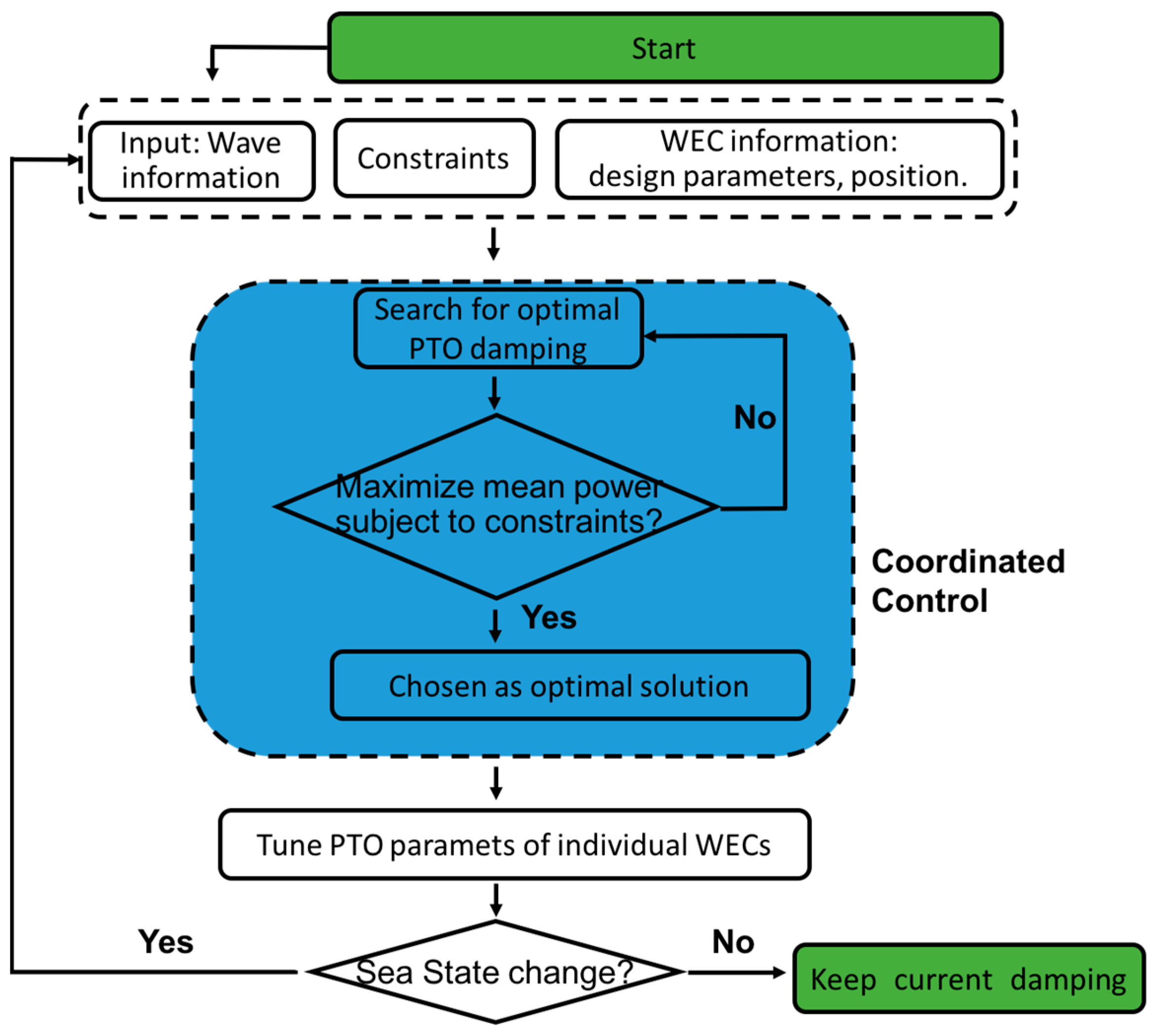
The scheme of the control method is shown in Figure 1. For each regular wave, the PTO damping of individual WECs will be coordinated. The hydrodynamic parameters, such as the added mass, damping coefficients, can be calculated by analytical methods or numerical methods. The numerical method is preferred in this paper.

2.4. Performance Evaluation

For the case in which only one WEC exists, no hydrodynamic cross-coupling will take place and its motion equation can be written as follows,

$${\displaystyle \sum }_{n=1}^6\left[-w^2\left(M_{n^{\prime }n}+m_{n^{\prime }n}\right)+iw\left(R_{n^{\prime }n}+C_{n^{\prime }n}\right)+S_{n^{\prime }n}+K_{n^{\prime }n}\right]{\widehat{x}}_n={\widehat{F}}_{e,n^{\prime }}$$

(18)

where $M_{n^{\prime }n}$, $m_{n^{\prime }n}$, $C_{n^{\prime }n}$, $S_{n^{\prime }n}$, $K_{n^{\prime }n}$, $R_{n^{\prime }n}$ are the elements of matrix $\mathit{M}$, $\mathit{m}$, $\mathit{C}$, $\mathit{S}$, $\mathit{K}$, $\mathit{R}$ representing the inertia matrix, added mass matrix, radiation damping matrix, hydrostatic matrix, PTO reactance matrix, PTO resistance matrix, respectively. The mean active power converted by this WEC, ${\overline{P}}_{single}$, can be calculated from Equation (12) while meeting the requirements of motion constraints, and will be used in the calculation of the Q factor.

The Q factor is a dimensionless parameter to evaluate the performance of the whole WEF, defined as the ratio of the total active power (mean value) converted by the WEF over the product of WEC numbers $N_C$ and power converted by an isolated WEC ${\overline{P}}_{single}$, written as

$$Q=\frac{{{\displaystyle \sum }}_p{\overline{P}}_p}{N_C{\overline{P}}_{single}}$$

(19)

Maximizing the energy production of the farm under the given sea state requires maximizing the Q factor.

3. Case Study

A small WEF consisting of four identical WECs based on the concept developed by Uppsala University is taken as an illustration in this section, and its performance using the CC method will be evaluated. The WEC has a semi-submerged buoy to absorb the wave energy and a linear generator to convert the absorbed energy into electricity. The buoy has small dimensions compared to the incident wave length, and belongs to the class of point absorber. The connection between the buoy and the generator is via a rope, which is modeled as a stiff rod. The performance of this WEC has been studied by numerical methods as well as real sea trials at the Lysekil test site [38,39,40].

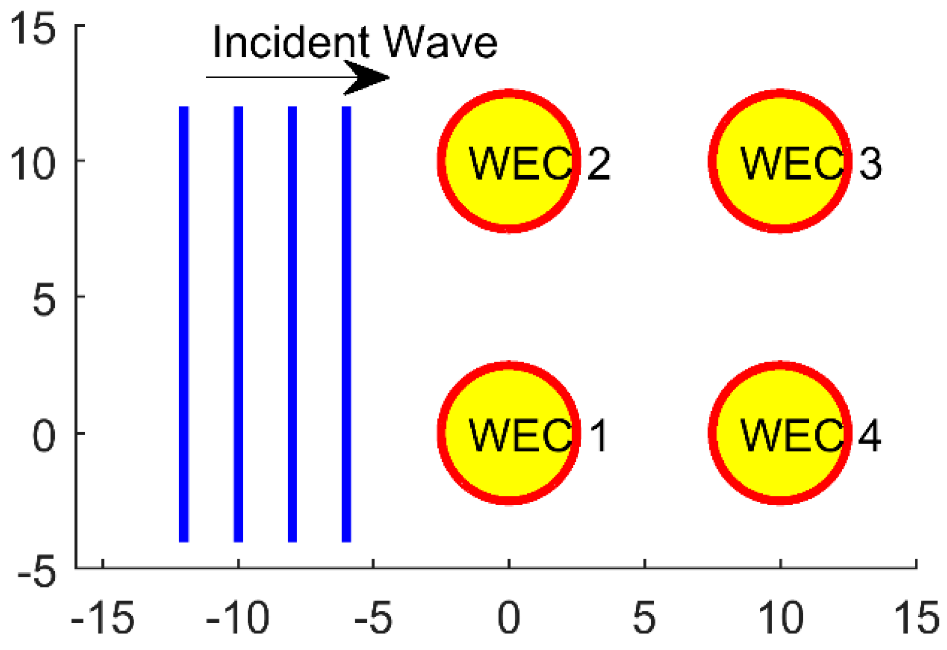
The layout of the farm is shown in Figure 2. Only one degree of freedom, the heave motion, is considered for each WEC. Therefore, a total of four degrees of freedom exists for this WEF system, denoted by $j=3,9,15,21$, and for the heave mode of WEC $p=1,2,3,4$, respectively.

To calculate the ${\overline{P}}_{single}$ in the Q factor, only the motion and power associated with the heave mode are considered, viz. $p=1,n=3,j=3$, and the motion equation can be expressed as follows:

$$\left[-w^2\left(M_{33}+m_{33}\right)+iw\left(R_{33}+C_{33}\right)+S_{33}+K_{33}\right]{\widehat{x}}_3={\widehat{F}}_{e,3}$$

(20)

The converted power can be written as

$${\overline{P}}_{single,3}=\frac{R_{33}}{2}{\left|{\widehat{u}}_3\right|}^2=\frac{\frac{{\left|{\widehat{F}}_{e,3}\right|}^2{R}_{33}}{2}}{{\left(R_{33}+C_{33}\right)}^2+{\left[w\left(M_{33}+m_{33}\right)-\frac{S_{33}+K_{33}}{w}\right]}^2}, \text{subject to} \{\begin{array}{c}\left|{\widehat{x}}_3\right|\le x_{3,max}\\ \left|{\widehat{u}}_3\right|\le w{x}_{3,max}\end{array}$$

(21)

As indicated by early research or can be seen from Equation (21), the value of PTO damping will influence the mean power converted by the isolated WEC, and therefore influence the value of the Q factor. In this paper, the maximum power converted by the isolated WEC will be found and used in the calculation of the Q factor.

It is well known that the maximum power of an isolated WEC in theory will be achieved in resonance. In the case when the motion is not constrained or the optimal motion amplitudes do not exceed the constraints, the maximum power can be described by

$${\overline{P}}_{single,3,max}=\frac{{\left|{\widehat{F}}_{e,3}\right|}^2{R}_{33}/2}{{\left(R_{33}+C_{33}\right)}^2}$$

(22)

However, sometimes the resonance condition cannot be achieved, such that the optimal displacement amplitude will be higher than the displacement limit. In such cases, the maximum converted power can be written as follows:

$${\overline{P}}_{single,3,max}=max {\overline{P}}_{single,3}\left(R_{33}\right), \text{subject to} \{\begin{array}{c}\left|{\widehat{x}}_3\right|\le x_{3,max}\\ \left|{\widehat{u}}_3\right|\le w{x}_{3,max}\end{array}$$

(23)

3.1. Coordinated Control

With the incident wave, four WECs will interact with each other. The motion of each WEC will produce a radiated wave, which will influence the heave motion of other WECs. Equation (10) can be written as

$$R_{p,33}{\widehat{u}}_j={\widehat{F}}_{e,j}+w^2{M}_{p,33}{\widehat{x}}_j-K_{p,33}{\widehat{x}}_j-S_{p,33}{\widehat{x}}_j-iw{\displaystyle \sum }_{j^{\prime }}{Z}_{j{j}^{\prime }}{\widehat{x}}_{j^{\prime }}$$

(24)

The total mean power converted by the WEF can be written as

$${\overline{P}}_{T,Nc=4}={{\displaystyle \sum }}_{p=1}^{Nc}\frac{1}{2}{R}_{p,33}{\left|{\widehat{u}}_j\right|}^2={{\displaystyle \sum }}_{p=1}^4\frac{1}{2}{R}_{p,33}{\widehat{u}}_j{\widehat{u}}_j^{*}={{\displaystyle \sum }}_{p=1}^4-\frac{1}{2}iw{\widehat{x}}_j^{*}[{\widehat{F}}_{e,j}+w^2{M}_{p,33}{\widehat{x}}_j-K_{p,33}{\widehat{x}}_j-S_{p,33}{\widehat{x}}_j-iw{{\displaystyle \sum }}_{j^{\prime }}{Z}_{j{j}^{\prime }}{\widehat{x}}_{j^{\prime }}]$$

(25)

The optimization problem is reformulated as

$$\mathrm{Maximize}{\overline{P}}_{T,Nc=4}\left({\widehat{x}}_{j=3},{\widehat{x}}_{j=9}, {\widehat{x}}_{j=15},{\widehat{x}}_{j=21}\right), \text{subject to} \{\begin{array}{c}\left|{\widehat{x}}_j\right|\le x_{j,max},j=3,9,15,21\\ \left|{\widehat{u}}_j\right|\le w{x}_{j,max},j=3,9,15,21\end{array}$$

(26)

where $x_{j,max}$ with $j=3,9,15,21$ indicates the maximum displacement amplitude of WEC $p$ with $p=1,2,3,4$ in heave mode.

3.2. Traditional Control

Here we define the use of a constant resistive load as traditional control (TC), and the same constant damping is used for each WEC. In this case, the power equation can be reformulated as

$${\overline{P}}_{T,tradi}={\displaystyle \sum }_{p=1}^{Nc}\frac{1}{2}{R}_{tr}{\left|{\widehat{u}}_j\right|}^2=\frac{1}{2}{R}_{tr}{\displaystyle \sum }_{p=1}^4{\left|{\widehat{u}}_j\right|}^2$$

(27)

where $R_{tr}$ is the PTO damping, which is same for each WEC. For the WEF with given incident wave, its performance will be influenced by the PTO damping. Different values of $R_{tr}$ will lead to different displacement amplitudes and energy production of the WECs. In this section, the optimal damping value $R_{tr,opt}$ will be calculated and used. Here, the optimal damping means the value to maximize the energy conversion of the WEF without violating motion constraints and can be expressed as follows:

$$R_{tr,opt}={}_{R_{tr}}{}^{argmax}(\frac{1}{2}{R}_{tr}{{\displaystyle \sum }}_{p=1}^4{\left|{\widehat{u}}_{p3}\right|}^2), \text{subject to} \{\begin{array}{c}\left|{\widehat{x}}_j\right|\le x_{j,max},j=3,9,15,21\\ \left|{\widehat{u}}_j\right|\le w{x}_{j,max},j=3,9,15,21\end{array}$$

(28)

3.3. Sea States and Parameters Used in Simulation

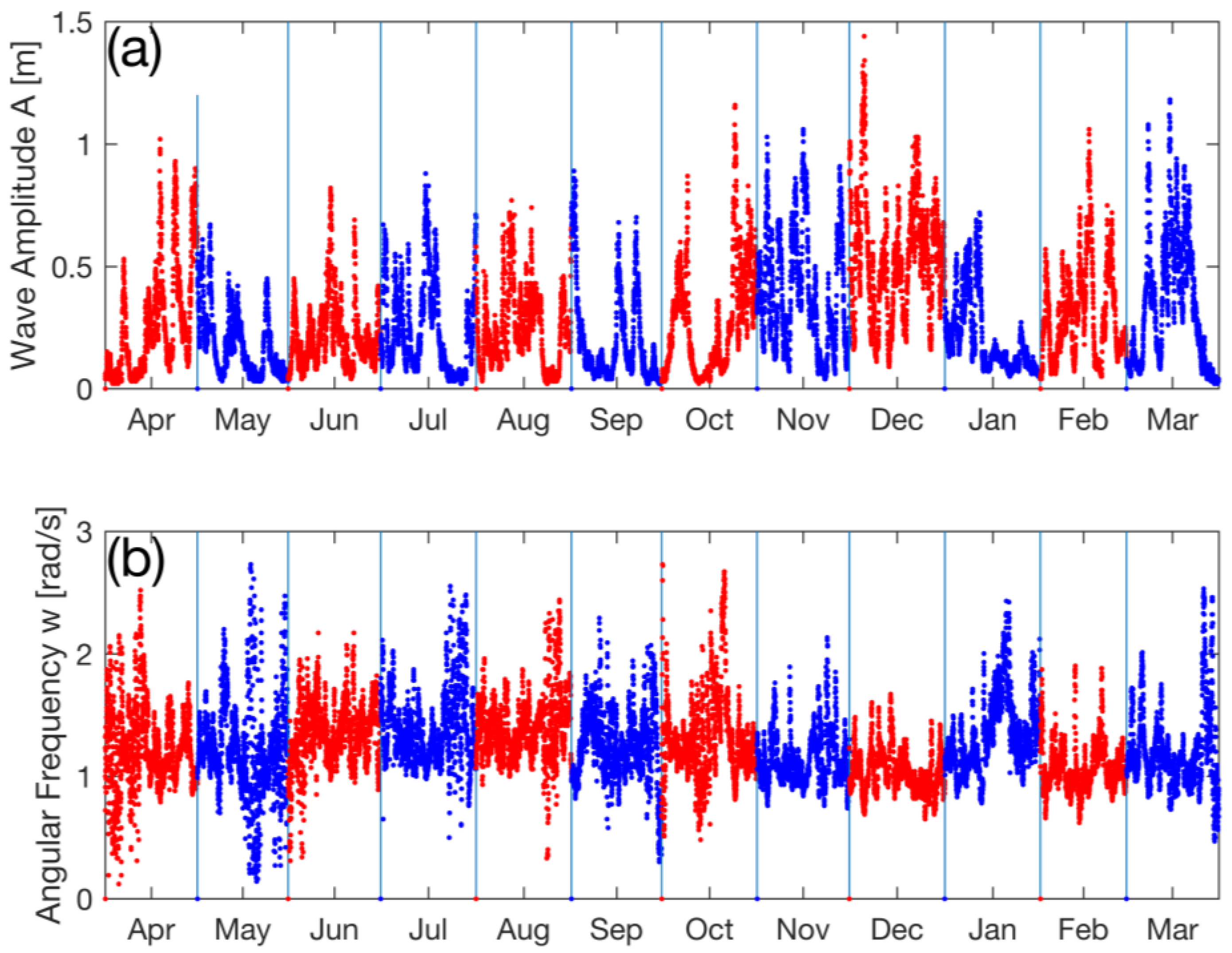
To evaluate the performance of a farm under the two control strategies in different regular waves, a scenario of wave data is created, as shown in Figure 3. This sea state used in the simulation are based on 12 months of measurement from April 2013 to March 2014 by a Waverider™ wave measurement buoy installed at the Lysekil test site. This involved the collection of 30 min time series of wave elevation sampled at 2.56 Hz, with a total of 17,134 time series (removed data are not included). These data are a reflection of the wave climate off the Swedish west coast, a location of a wave energy research site run by the Centre for Renewable Electric Energy Conversion at Uppsala University. This site has had a wave power plant installed since the spring of 2006 [41].

For a deep-water sinusoidal wave with amplitude of $h$ and period of $T$, the power level can be expressed as [42]

$$J=\frac{\rho g^{2}T{\mathrm{h}}^2}{32\pi }$$

(29)

The buoys have a radius of 2.0 m and draft of 0.5 m. Intervals for the control strategies are set to 30 min to coincide with the wave elevation time series. Hydrodynamic coefficients are calculated in WAMIT [43], and the optimization problem is solved in MATLAB based on the fmincon function. The main parameters used in the simulations are shown in

Table 1. Parameters used in case study.

Parameter	Value
WEC radius	2 m
WEC draft	0.5 m
${\mathrm{M}}_{\mathrm{p},33}, \text{where p}=1,2,3,4$	6434 kg
${\mathrm{K}}_{\mathrm{p},33}, \text{where p}=1,2,3,4$	5 kN/m
${\mathrm{x}}_{\mathrm{j},\text{max}},j=3,9,15,21$	1 m
Water depth	20 m
WEC 1 coordinate	(0, 0)
WEC 2 coordinate	(0, 10)
WEC 3 coordinate	(10, 10)
WEC 4 coordinate	(10, 0)

.

3.4. Results and Analysis

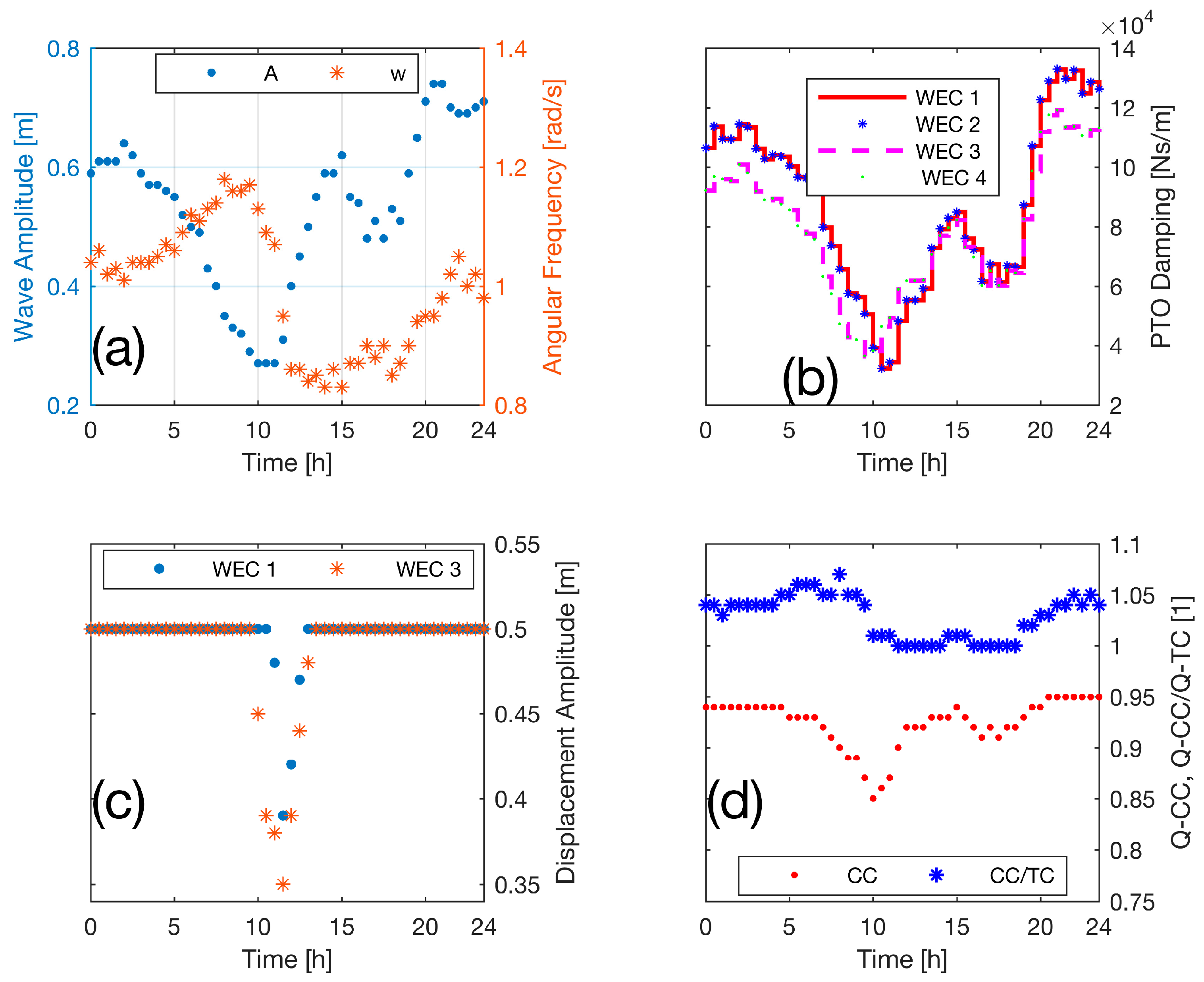
Sea states for a selected time window of 24 h are presented in Figure 4a. It is related to the sea states of 16 March 2014, also shown in Figure 3. Each point represents the sea states of 30 minutes, and there are 48 sea states in this period of 24 h. The wave amplitude varies in the range of 0.27 m–0.74 m. The angular frequency of the incident wave is in the range of 0.83 rad/s–1.18 rad/s, corresponding to a period of 5.32 s–7.57 s.

Figure 4b illustrates the optimal PTO damping for the WECs using CC versus time. WEC 1 and WEC 2 have same optimal damping in all sea states, and WEC 3 and WEC 4 also have the same situation. This is due to the fact that the incident angle of all incident waves are assumed to be zero in the simulation, resulting in the symmetry of the WEC 1 and WEC 2, or WEC 3 and WEC 4, with respect to the centerline of the WEF parallel to the incident wave direction. It should be noted that the optimal PTO damping for different WECs is sensitive to the sea states, and it can be same or largely different. The maximum value of optimal PTO damping is 133 kNm/s, while the minimum is 32 kNm/s.

Figure 4c shows the optimal displacement amplitudes of WECs using CC. For most sea states (41 in total), all WECs have a displacement amplitude of 0.5 m, the same as the displacement constraint. When the wave amplitude reaches 0.27 m, the minimum value within 24 h, the displacement of WEC 3 drops quickly, and this continues with the decrease of the angular frequency of the incident wave. After that, the displacement amplitude increases with the wave amplitude when the angular frequency of the incident wave fluctuates in a narrow range and becomes 0.5 again. WEC 1 shows the same pattern, only smoother.

Figure 4d plots the Q factor of the WEF using CC, as well as the ratio of Q factors using two different control strategies. Note that the trend of the Q factor cannot be predicted directly based on the sea states from this figure. Since both the numerator and denominator of Equation (19) vary with sea states. Their ratio, the Q factor, can vary with sea states or not. We can also see that the Q factor from CC control varies in the interval of [0.85,0.95], lower than 1, which indicates that the wave interactions have a destructive effect on the energy conversion of the WEF. Another line in this figure, the comparison of two strategies, indicates that the CC can give a higher power production for the WEF in most sea states in this 24-hour interval, and this improvement can sometimes be up to 7.0%.

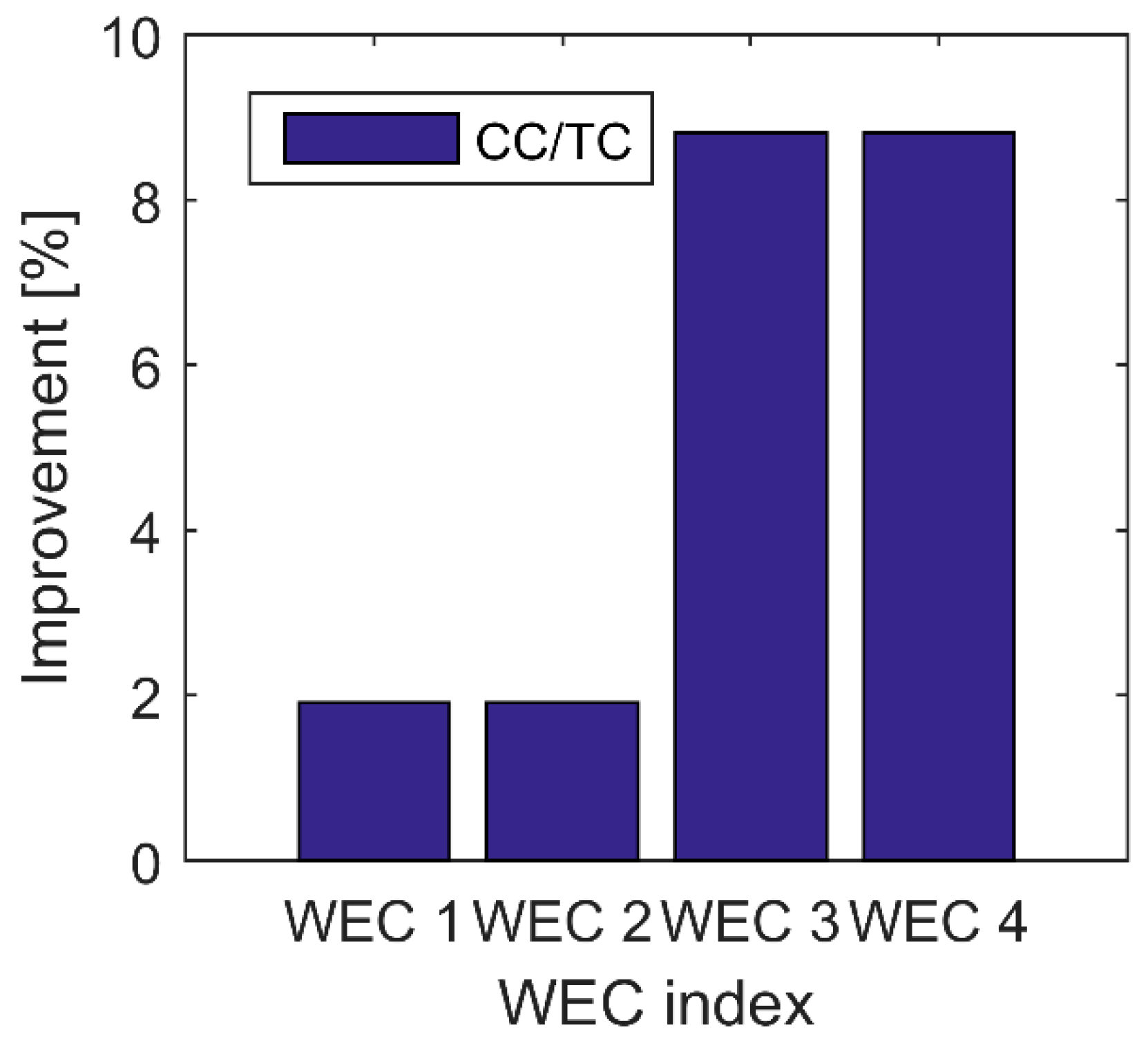
The benefits of the CC compared with TC are also shown in Figure 5 and Figure 6. Figure 5 shows the total improvement of energy conversion in 12 months for each WEC. For WEC 1 and WEC 2, the CC can improve the energy production by about 2.0%. For WEC 3 and WEC 4, this performance can be improved by 8.8%. This indicates that the CC can decrease the shadowing effect and improve the performance of the shadowed WECs.

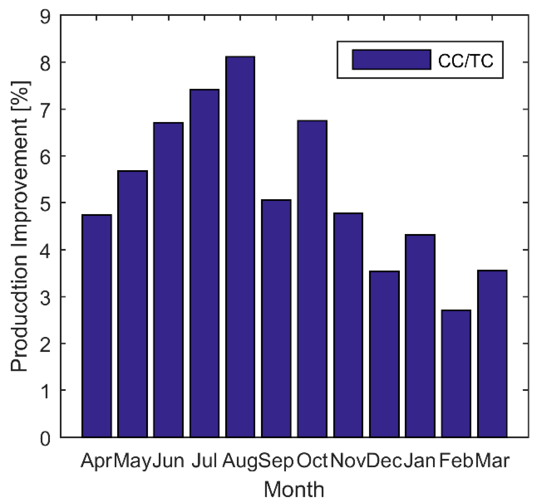
From Figure 6, the production improvement of the whole farm in each month can be seen clearly. For April, the production of the farm can be improved 4.74% by using the CC method compared to that using TC. This ratio increases gradually and reaches the maximum value of 8.11% in August. After that, it decreases to the minimum value of 2.71% in February. As stated before, the performance improvement caused by the CC control method can be influenced by the sea states, and this will also be explained in Figure 7.

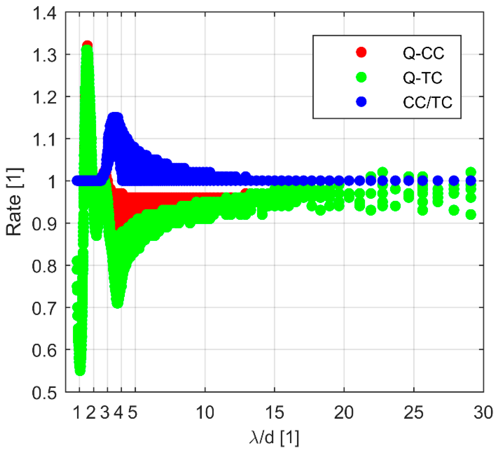
Figure 7 shows the Q factors of the WEF using two different control methods, as well as the ratio of two Q factors. The results include Q factor information of 12 months. It is found that, no matter which control method is used, the Q factor is sensitive to the incident wave length when the wave length is less than 15 times the gap distance between WECs. The Q factors have the lowest values when the incident wave length λ equals the gap distance, and the highest values when the wave length is 1.5 times the gap distance. The second trough, second peak and third trough of the Q factor line occur when the wave length is about 2.0, 2.5, 4.0 times the gap distance, respectively. After that, the trend line tends to be stable, and close to 1. It can also be seen that, when λ/d is too small or too large, the ratio of two Q factors is 1, which indicates that the performance of the WEC cannot benefit from the CC. However, when the ratio of the incident wave length and the gap distance is in the interval [3,6], the ratio of two Q factors is larger than 1, with the maximum value of 1.15, which means that the performance of the WEF can be strongly improved by the CC in this range.

4. Conclusions

Considering the hydrodynamic interaction of the WECs, as well as the motion constraints, a new control strategy coordinating the PTO damping of each WEC is described in this paper. The optimal PTO damping for each WEC are found in given sea states, which are different for shadowed and non-shadowed wave energy converters. The optimal PTO damping for each wave energy converter varies over sea states and influences the motion of converters as well as the hydrodynamic interaction between them.

Results indicate that, with the optimal PTO damping, the displacements of all converters will be the same as the displacement constraint value in some sea states. The performance of the shadowed wave energy converters can be improved significantly, with an average improvement of 8.8% compared with the TC method in the given sea states of 12 months. The performance of the whole wave energy farm can also be improved by this coordinated control method.