Article

Techno-Economic Planning of a Fully Renewable Energy-Based Autonomous Microgrid with Both Single and Hybrid Energy Storage Systems

1
Department of Electronic and Electrical Engineering, University of Sheffield, Sheffield S10 2TN, UK
2
Sheffield University Management School, University of Sheffield, Sheffield S10 2TN, UK
3
School of Engineering, University of Southampton, Southampton SO17 1BJ, UK
*
Author to whom correspondence should be addressed.
Energies 2024, 17(4), 788; https://doi.org/10.3390/en17040788
Submission received: 16 January 2024 / Revised: 2 February 2024 / Accepted: 5 February 2024 / Published: 6 February 2024
(This article belongs to the Special Issue Hybrid Battery Energy Storage System)

Abstract

:
This paper presents both the techno-economic planning and a comprehensive sensitivity analysis of an off-grid fully renewable energy-based microgrid (MG) intended to be used as an electric vehicle (EV) charging station. Different possible plans are compared using technical, economic, and techno-economic characteristics for different numbers of wind turbines and solar panels, and both single and hybrid energy storage systems (ESSs) composed of new Li-ion, second-life Li-ion, and new lead–acid batteries. A modified cost of energy (MCOE) index including EVs’ unmet energy penalties and present values of ESSs is proposed, which can combine both important technical and economic criteria together to enable a techno-economic decision to be made. Bi-objective and multi-objective decision-making are provided using the MCOE, total met load, and total costs in which different plans are introduced as the best plans from different aspects. The number of wind turbines and solar panels required for the case study is obtained with respect to the ESS capacity using weather data and assuming EV demand according to the EV population data, which can be generalized to other case studies according to the presented modelling. Through studies on hybrid-ESS-supported MGs, the impact of two different global energy management systems (EMSs) on techno-economic characteristics is investigated, including a power-sharing-based and a priority-based EMS. Single Li-ion battery ESSs in both forms, new and second-life, show the best plans according to the MCOE and total met load; however, the second-life Li-ion shows lower total costs. The hybrid ESSs of both the new and second-life Li-ion battery ESSs show the advantages of both the new and second-life types, i.e., deeper depths of discharge and cheaper plans.

1. Introduction

The number of electric vehicles (EVs) is expected to increase significantly in developed countries to both decrease fossil fuel usage and achieve healthier and less polluted air in urban areas. This is supported by government policies on different scales. As an example, the United Kingdom (UK) government announced that all new passenger cars will be zero-emissions vehicles (ZEVs) at the tailpipe from 2035 to reduce the transport sector emissions [1], which is now the highest emitting sector in the UK, having overtaken the energy sector [2]. Additionally, the UK’s introduction of the ZEV mandate in 2024 requires car manufacturers to increase their percentage of ZEV’s sold as new vehicles per year [3]. However, to maximise the impact of the decarbonisation of road transport, EVs alone are not enough, particularly whilst they are supplied by an electricity grid that still relies heavily on fossil fuel-based power plants. The second necessity to completely achieve the above-mentioned goal of decarbonisation is to ensure that EVs are supplied electricity from renewable energy resources (RESs). However, connecting a large number of EVs to the electricity grid causes a considerable increase in the load demand, overloading various components of the power grid, changing load profile patterns, distorting the voltage or frequency of the grid, and generating power system imbalances [4]. Therefore, RES-oriented off-grid EV charging stations, which form autonomous microgrids (MGs), provide a good solution to address these current EV/grid challenges.
The Future Electric Vehicle Energy networks supporting Renewables (FEVER) project [5] is investigating solutions to develop autonomous EV charging MGs, where energy storage systems (ESSs) are necessary to compensate for renewable energy source (RES) uncertainties. A combination of RESs and ESSs is needed to provide a level of reliability, availability, and flexibility to the issue of charging EVs. However, it is crucial to properly size various components of these systems to avoid excessive costs for the system and to minimize the amount of load not being met by generation sources such as PV systems and wind turbines [6].
The sizing/planning of the main MG modules is the first step to designing and implementing EV charging MGs to be sure to achieve the best plans, considering both technical and economic aspects. Different approaches and software packages have been used for MG planning in the literature. HOMER is a software package specially designed for MG planning studies [7], which can model different types of RESs, ESSs, and loads [8]. In [9], a scheme is presented for EV charging station planning for a remote microgrid. However, fossil fuel-based generation systems are involved in the planning, and the amount of greenhouse gas emission is considered as an objective function in addition to the planning costs. Optimal battery planning is presented in [10] for a microgrid, assessing the state of health (SOH) of the batteries. The authors used two types of technologies, including lithium-ion (Li-ion) and lead–acid (LA) batteries, for the proposed solution. A two-stage planning scheme is presented in [11] for sizing batteries in a microgrid, where, in the first stage, the size and maximum depth of discharge are extracted, and in the second stage, an appropriate battery technology is chosen. In addition to planning costs, system reliability is also investigated in [12]. Nonetheless, once again, the authors assumed diesel generation systems that lead to greenhouse gas emissions.
Hybridizing ESSs is a solution to obtain a more reliable and flexible off-grid MG, particularly since a hybrid ESS (HESS) can achieve a higher SOH than that of an individual ESS unit [13,14]. Various types of energy storage systems have different advantages in terms of cost, longevity, capacity, and response time. Another FEVER case study has been investigated for an MG, including a Li-ion battery ESS and a supercapacitor ESS, in terms of technical modelling and planning [15]. The utilisation and the economics of renewable energy have been enhanced by considering a HESS, as shown in [16]. Planning costs are illustrated to decrease in [17] by utilising a HESS, when compared to the case that merely relies on Li-ion batteries. The utilisation of both Li-ion and lead–acid batteries is reported in [18] for stationary applications, and the relative benefits of each of these technologies are discussed. Also, the concurrent use of Li-ion and lead–acid batteries is also reported in [19] for microgrid applications. Another FEVER case study has covered the DC coupling of Lithium-ion and lead–acid batteries in a HESS, which showed that in a fully optimised generation and battery storage scenario, the hybrid system alone could further reduce the overall system cost by 10% [20].
In recent years, second-life batteries have also been studied as an option to be deployed in a HESS. These are typically EV batteries that have lost almost 20% of their original capacity and can be used for stationary applications in stand-alone energy systems based on renewable generation due to their lower costs and capabilities for harnessing volatility and interrupted performance for these generation sources [21]. In [22], the authors investigate the possibility of reusing battery cells after vehicle use for an energy grid and show the environmental advantages of this utilisation. Batteries retired from EVs are proposed for a large stand-alone MG composed of EV charging stations, PV generation systems, and second-life batteries [23]. The results of this research illustrate a decreased operational cost for the system by using second-life batteries of EVs alongside new batteries in a twenty-year planning period. However, using only second-life batteries in such a large MG is not reasonable due to the high replacement costs and sharp increases in power losses during charging/discharging. The application of second-life batteries has also been investigated for ancillary services for grids [24]. The results in this reference illustrate how their usage can lead to the reduction in EV prices and an increase in the advantages of electrifying the transportation sector. Centralized charging stations were planned in [25] based on second-life batteries, where the researchers used an optimized charge/discharge approach to increase the lifetime of these batteries.
This paper presents a sensitivity analysis-based techno-economic planning of off-grid renewable-supplied MGs employed for electrifying EV charging stations using the MCOE and considering both single and hybrid ESSs. The major contributions of this paper are as stated below:
  • A general power-in-power-out model of ESSs is extended for long-term studies, e.g., the sizing and planning of ESSs, which is also improved in terms of the local energy management system (EMS) against the original model [26].
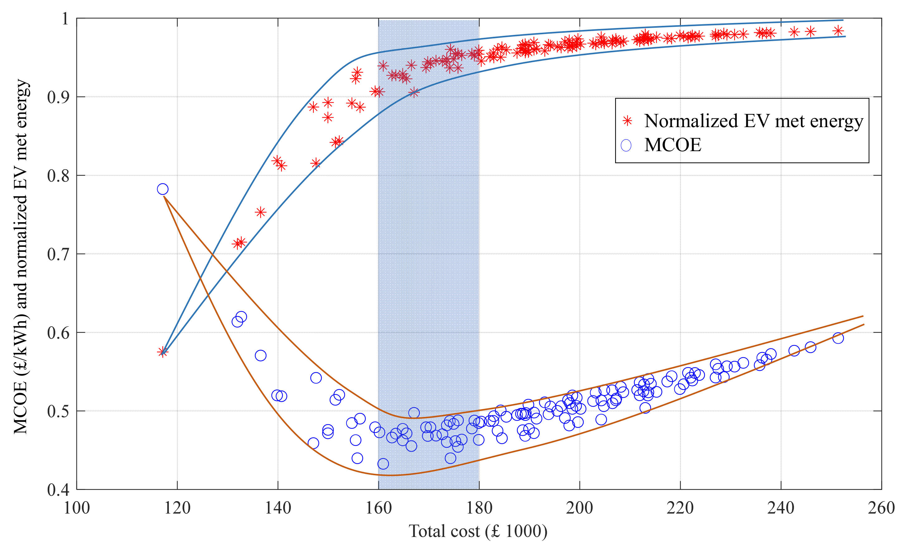
  • A modified COE (MCOE) is proposed as the main characteristic to compare different plans including the main terms of COE, i.e., total costs and total provided energy for the EV demand, and two added terms including the present value of ESSs and the EV unmet energy, i.e., the EV energy demand that could not be supplied by either RESs or ESSs. The first additional term helps to make the economic analysis free from the ESS lifetime, and the second increases the weighting coefficient of the technical aspect in the techno-economic sizing and decision-making.
  • Sensitivity analysis is used for both single and hybrid ESSs to compare different combinations of participants in the techno-economic planning studies. In the single-ESS studies, the feasible search space is composed of the number of wind turbines, the number of solar panels, and the single-ESS nominal capacity, and in the HESS studies, it includes the nominal capacity of different ESS battery technologies. The sensitivity analysis-based planning provides several suitable plans with reasonable conditions.
  • The impact of the global EMS strategy of the HESS on the techno-economic characteristics is studied, where a power-sharing-based EMS is developed to be compared with a simpler logic-based EMS.
The rest of this paper is organized as follows. Section 2 presents the technical and economic modelling methods of the studied autonomous MG. Section 3 represents the sensitivity analysis-based planning method of the MG. Section 4 addresses the simulation results and the corresponding discussions. In Section 5, the key findings and results of the study are summarized.

2. Techno-Economic Modelling

An off-grid EV charging station can be assumed as an autonomous MG since it includes the main components of an MG, namely, generation units, storage units, load, and control and protection infrastructure to operate the MG stably and securely. Figure 1 shows a schematic of the studied MG, including solar energy and wind energy generation units, HESS, some EV charging points, and required power conversion devices to connect all modules to a common ac bus.
As an example, a general outdoor ground-level car park where there is sufficient area to build the charging station is considered. However, space management is critical in a real project, especially one constructed in an urban area, because the targeted car parks would not be typically designed for an EV charging station from the outset. This limits the size of potential renewable energy generation technologies as well as the types of ESS deployed.
Since wind and solar energies are available for most of the potential locations considered for an off-grid EV charging station MG in the UK, they are preferred as renewable energy sources in the planning study. The weather data required for RES generation prediction and modelling are obtained at the target location, which is a visitor attraction in Southern England. Different combinations of various available ESS technologies can be used to provide suitable power density and energy density for the studied MG. However, in this paper, the HESS is assumed to consist of a combination of three battery ESS technologies consisting of a new Li-ion ESS, a second-life Li-ion ESS, and a new lead–acid ESS to compare in different plans. Moreover, battery ESSs are easy to install and require a ground level as close as possible to the car park, which is important in this study to decrease cable losses.
Note that both the technical and economic models of the MG were required for the techno-economic analysis performed in this study. The technical modelling of the system addresses power flow modelling, where details of currents and voltages are not required. Therefore, detailed models of power converters, which are usually used in dynamic studies, are not taken into account here but are rather considered as efficiency blocks denoting a loss contribution.

2.1. Technical Modelling

Figure 2 shows all MG modules that should be modelled and their interrelationships. Three data sets are required to model the renewable energy generation units and EV charging station demand: these are solar radiation, wind speed, and the number of visiting vehicles along with their arrival times. Modules of the studied MG include an EV charging station demand, a wind generation unit, a solar generation unit, the HESS EMS, and ESSs, which are modelled in the next subsections, and then a comprehensive technical model of the MG is obtained by connecting the individual module models.

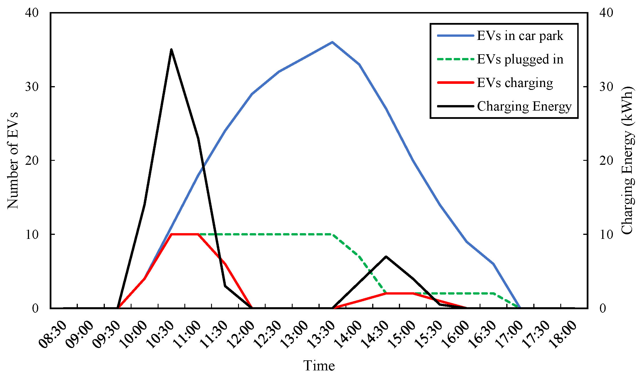
2.1.1. EV Demand Power

To determine the normal EV loading on the system, it is possible to examine typical travel profiles for car park users at the visitor attraction, which is assumed to be open from 10.00 until 17.00 on working days. These opening times set a boundary for when EVs can plug in and charge at the car park. The EV charging station is modelled assuming 10 ac chargers with a power rating of 7 kW and rated voltage of 240 V each. Therefore, the charging station is classified as level II. The daily energy load demand for charging the EVs is then calculated using the chargers’ usage profile based on data regarding the total number of vehicles arriving at the car park each day in 2019, and the hourly vehicle arrival profile. The model then calculates the number of EVs arriving at the car park, assuming 3% of the total car arrivals are EVs according to recent EV statistics in the UK [27].
Cars are assumed to be parked for 4 h based on typical customer dwell times at the visitor attraction; thus, 4 h is used in this model as the plug-in period for each EV if any of the 10 chargers are unoccupied when arriving at the car park. The model assumes the average efficiency of an EV is 4 miles per kWh, and each vehicle needs to charge to cover a total distance of 30 miles, which is determined to be the average customer distance travelled to the visitor attraction. Figure 3 shows typical EV behaviour at the car park and EV charging demand for a single day. Hourly charging energy demand provides the EV demand power, P e v , in hourly steps, which can easily be converted to a second-by-second power signal.

2.1.2. Wind Generation Power

Electrical yield is calculated from wind speed data [28] by first converting them from the measurement height to the generator’s hub height. The log law is used here as it delivers consistent results up to a height of 20 m above ground level, and a 20 m wind turbine is chosen for the EV charging station as a small wind turbine suitable for MG applications:
U z = U z , r e f × ln z z 0 / l n ( z r e f z 0 ) ,
where z and z r e f are new height (m) and reference height (m), respectively, and U z and U z , r e f are mean wind speed at the new height (m/s) and mean wind speed at the reference height (m/s), respectively. z 0 is surface roughness length (m). Surface roughness is a value based on the protrusion of land cover, e.g., grass, trees, buildings.
Next, wind yield (kWh) is calculated by the interpolation of the manufacturer’s power curve (kW), which is based on verified measurements. In this study, the Aventa AV-7 WT power curve is used, with a rated power of 6.2 kW, as follows [29]:
P w t = 0 ,                                                                                                       U z < 2   o r   U z > 14     0.36 × U z 2 1.48 × U z + 1.72 .         2 U z 6.17 6.2 ,                                                                                                     6.17 < U z 14

2.1.3. Solar Generation Power

To model the solar generation power, a photovoltaic geographical information system [28] is used to obtain hourly data of three main components of the solar irradiance on the inclined plane in k W / m 2 , i.e., diffuse irradiance ( I d i f ), direct irradiance ( I d i r ), and ground-reflected irradiance ( I r e f ). It is assumed that the slope and azimuth have been optimised to obtain the maximum solar irradiance at the target location. Therefore, the total irradiance on the inclined plane ( I t o t ) can be obtained as follows:
I t o t = I d i f + I d i r + I r e f .
The hourly solar generation power ( P p v ) can easily be calculated as below:
P p v = I t o t × η i × η p × p d × N p v ,
where η i is the PV converter efficiency, η p is the panel efficiency, p d is the panel dimension m 2 , N p v is the number of panels, and P p v is obtained in k W .

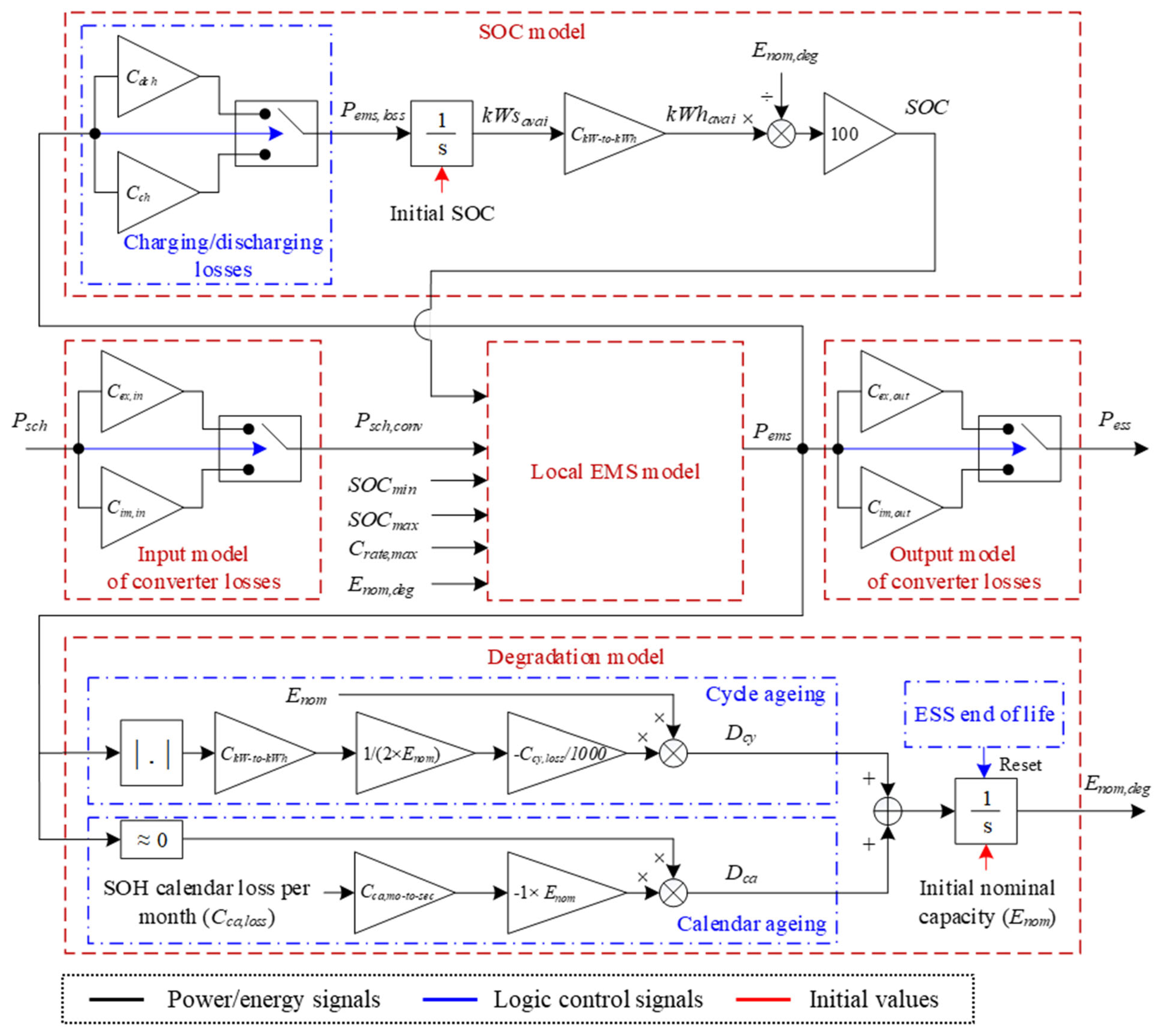
2.1.4. ESS Power-in-Power-out Model

The ESS model is an extension of the power-in-power-out model presented in [26], which provides long-term MG modelling and is required for planning and sizing studies. Figure 4 shows a comprehensive schematic of this enhanced power-in-power-out ESS model, including five main parts indicated by red dashed boxes, namely, input model of converter losses, local EMS model, output model of converter losses, SOC model, and degradation model.
Input model of converter losses: The scheduled power of the ESS, P s c h , determined by the HESS EMS is the main input of the ESS model, where it is the input of the converter losses model block inside the ESS model. This block includes two different gains as power converter loss coefficients for power import and power export situations, i.e., C i m , i n and C e x , i n , where C i m , i n = 1 K c o n v , l o s s / 100 , C e x , i n = 1 / ( 1 K c o n v , l o s s / 100 ) , and K c o n v , l o s s is the converter export/import power loss parameter, which is usually less than 10%. The scheduled power after assuming input converter losses, P s c h , c o n v , is obtained according to the sign of the scheduled ESS power as follows:
P s c h , c o n v = C e x , i n × P s c h ,     P s c h 0 C i m , i n × P s c h .     P s c h < 0
Local EMS model: The P s c h , c o n v is assumed as an input for the local EMS model to calculate the allowable amount of power charged/discharged by the ESS, P e m s , considering the allowable band of the SOC determined by S O C m i n and S O C m a x , and maximum c-rate, C r a t e , m a x . In fact, two conditions should be satisfied at every time step:
S O C m i n S O C S O C m a x , P e m s P r a t e d ,
where P r a t e d is the allowable rated power usually assumed to be calculated as
P r a t e d = C r a t e , m a x × E n o m , d e g ,
where E n o m , d e g is the degraded nominal capacity obtained from the degradation model (see Figure 4). However, the allowable rated power is not only influenced by the maximum c-rate but is also affected by the maximum allowable charging/discharging power based on the difference in SOC from the S O C m i n or S O C m a x in each sample time of the model simulation. This power can be calculated as follows:
P s o c , m a x c h , m a x = S O C m a x S O C 100 × E n o m , d e g × 3600 T s a m p l e , P s o c , m i n d c h , m a x = S O C S O C m i n 100 × E n o m , d e g × 3600 T s a m p l e ,
where T s a m p l e is the sample time of the model simulations, and E n o m , d e g is the degraded nominal capacity of the ESS in kWh, which is obtained as the output of the degradation model. P s o c , m a x c h , m a x is the maximum allowable power change during charging limited by maximum SOC at each sample time in kW/sample time, and P s o c , m i n d c h , m a x is the maximum allowable power change during discharging limited by minimum SOC at each sample time in kW/sample time. Therefore, one can represent the improved allowable rated powers, P r a t e d , i m p c h and P r a t e d , i m p d c h , during charging and discharging, respectively, as follows:
P r a t e d , i m p c h = m i n ( P r a t e d , P s o c , m a x c h , m a x ) , P r a t e d , i m p d c h = m i n ( P r a t e d , P s o c , m i n d i s c h , m a x ) ,
where min(.) indicates finding the minimum of the input argument. Finally, P r a t e d is replaced by P r a t e d , i m p c h or P r a t e d , i m p d c h in (6), and conditions in (6) are applied in the local EMS model using logic rules to assume the maximum allowable part of the P s c h , c o n v as the output power, i.e., P e m s .
SOC model: As shown in Figure 4, the SOC model block uses P e m s from the local EMS model and E n o m , d e g from the degradation model to calculate the SOC as follows:
S O C = C k W t o k W h × P e m s , l o s s d t E n o m , d e g × 100 ,
where C k W t o k W h is 1/3600 to convert the available ESS energy in kWs to the available ESS energy in kWh, and P e m s , l o s s is obtained from the P e m s after applying charging/discharging losses as follows:
P e m s , l o s s = C d c h × P e m s ,     P e m s 0 C c h × P e m s ,     P e m s < 0
where C d c h = 1 K c h , l o s s / 100 , C c h = 1 + K c h , l o s s / 100 , and K c h , l o s s is the charging/discharging loss parameter, which can yield different percentage values according to the ESS technology (see Table 1).
Degradation model: In the degradation model shown in Figure 4, cycle ageing and calendar ageing are modelled through their equivalent degradation terms, namely, D c y and D c a , as follows:
D c y = C k W t o k W h × P e m s 2 E n o m × C k W t o k W h × P e m s × ( C c y , l o s s / 1000 ) ,
D c a = C c a , l o s s × C c a , m o t o s e c × E n o m ,   P e m s 0
where the first term of (12) calculates the equivalent cycles of charging/discharging according to micro-cycling, and C c y , l o s s is the SOH loss parameter per 1000 cycles. The terms in (13) are as follows: C c a , l o s s is the SOH calendar loss per month, and C c a , m o t o s e c is a coefficient to convert the calendar loss per month to the calendar loss per second. Note that the calendar losses are assumed to only occur during storing times, when P e m s 0 , i.e., when ESS is not in use. Therefore, the degraded nominal capacity of the ESS can be calculated as follows:
E n o m , d e g = ( D c y + D c a ) d t .
Note that the ESS end-of-life can be modelled as a percentage of the nominal ESS capacity, where it is compared with the degraded capacity. When the degraded capacity decreases to the end-of-life value (see Table 1), a logic signal resets the integrator used in the degradation model.
Output model of converter losses: The last part of the ESS model is the output model of the converter losses, which has the same structure as the input model of the converter losses. Therefore, the output ESS power, P e s s , can be obtained as follows:
P e s s = C e x , o u t × P e m s ,     P e m s 0   ( d i s c h a r g e ) C i m , o u t × P e m s ,     P e m s < 0   ( c h a r g e )
However, the converter loss coefficients for power import and power export situations in the output model, i.e., C i m , o u t and C e x , o u t , have different relationships as follows:
C i m , o u t = 1 / ( 1 K c o n v , l o s s / 100 ) , C e x , o u t = 1 K c o n v , l o s s / 100 .              
The enhanced ESS model can be utilised for different types of electrical and electro-chemical ESSs without any structural changes and by only assuming suitable parameters, which are obtained here using some experimental tests and validated models in the literature [30,31,32]. Table 1 shows the parameters for the studied hybrid ESS, including the new and second-life Li-ion battery ESSs and the new lead–acid battery ESS. The second-life Li-ion battery ESS is made up of second-life modules, which are tested to select healthy, reduced-capacity modules to prevent possible variability and nonlinearity in their performance and, thus, provide a reliable ESS.

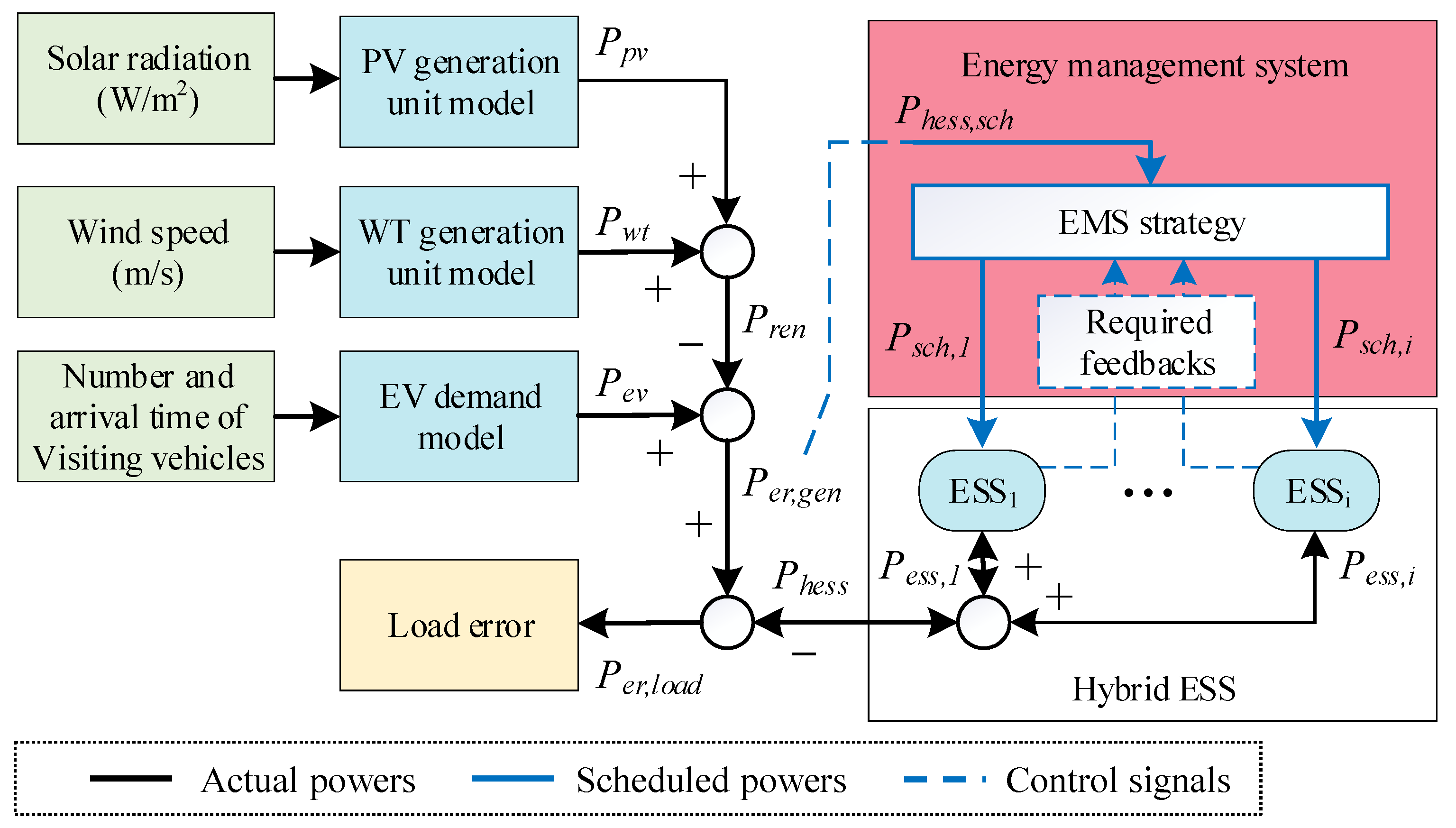
2.1.5. HESS Energy Management Model

Here, a two-level energy management system is used, i.e., local and global EMSs. The first level, i.e., the local EMS, is performed separately for each ESS as explained in Section 2.1.4. The second level, i.e., the global EMS, determines the share of the HESS scheduled power, P h e s s , s c h , for each ESS, i.e., P s c h , 1 ,…, P s c h , i (see Figure 2). To this end, it requires some information of each ESS whose type depends on the EMS strategy. Here, two different strategies are considered for the global EMS to show the impact of the global EMS on the MG planning results, including a HESS. A priority-based EMS and a power-sharing-based EMS are studied.
Priority-based EMS: In this type of global HESS EMS, a very simple logic rule is considered to apply a priority between different ESSs for charging and discharging. Due to the features of the studied ESSs such as depth of discharge (DOD), SOH, and the end of life, the new Li-ion battery ESS is considered the first priority, and the second-life Li-ion battery ESS and the new lead–acid battery ESS are assumed to be the second and third priorities for charging/discharging, respectively. Although this global EMS has a very simple structure and does not need input signals, e.g., SOC and SOH, it may be very far from optimised management due to its inability to consider details of the ESSs to charge or discharge them. To implement the priority-based EMS, the difference between the ESS scheduled power and the ESS real power of the higher priority at each sample time, i.e., P s c h , i ( t ) P e m s , i ( t ) , is assumed as the scheduled power of the lower priority as follows:
P s c h , 2 ( t ) = P s c h , 1 ( t ) P e m s , 1 ( t ) ,
P s c h , 3 t = P s c h , 2 t P e m s , 2 t ,
where 1, 2, and 3 in subscripts are used for the first, second, and third priorities of ESSs, respectively.
Power-sharing-based EMS: In this strategy, more details of the ESSs’ information are used in the global EMS to improve their SOH. Moreover, different charging and discharging rules are used to satisfy these situations with their required input data. The main idea is to compare the DOD and maximum c-rate of the ESSs during charging and to compare the SOC and maximum c-rate of the ESSs during discharging to share the HESS scheduled power among the ESSs.
The charging rule is to consider the empty ESS capacity according to DOD and the maximum c-rate of participating ESSs during charging, which is converted to the equivalent power. To this end, the charging parameters are determined as follows:
K c h , i = C r a t e , m a x i × E n o m , d e g , i × D O D i % 100 ,
where K c h , i is the charging parameter of the i-th ESS. Hence, the charging power share of the i-th ESS can be calculated using a sharing rule as follows:
P s c h , i = K c h , i i K c h , i × P h e s s , s c h ,
where P h e s s , s c h and P s c h , i are the negative values of the HESS scheduled power and the i-th ESS scheduled power. Therefore, ESSs, which have greater charging parameters, participate in charging with greater shares. This helps to improve SOH by increasing small SOCs of the ESSs, which results in smaller cycle ageing.
The discharging rule is to consider the available ESS power according to the SOC and the maximum c-rate of participating ESSs in discharging. This available power for discharging is calculated using a discharging parameter, which can be obtained as follows:
K d c h , i = C r a t e , m a x i × E n o m , d e g , i × S O C i % 100 ,
where K d c h , i is the discharging parameter of the i-th ESS. The discharging power share of the i-th ESS can be calculated as follows:
P s c h , i + = K d c h , i i K d c h , i × P h e s s , s c h + ,
where P h e s s , s c h + and P s c h , i + are the positive values of the HESS scheduled power and the i-th ESS scheduled power. Therefore, the ESSs with greater discharging parameters participate in discharging with greater shares. This improves SOH by decreasing the high SOCs of the ESSs during discharge, which causes more calendar ageing if they are maintained.
After determining the scheduled power of each ESS according to (17) and (18) for the priority-based EMS or (20) and (22) for the power-sharing-based EMS, it is considered as the input of the ESS model indicated by P s c h in Figure 4. Finally, as shown in Figure 2, the actual HESS output is obtained by summing the actual output of all ESSs as follows:
P h e s s = i = 1 N P e s s , i .

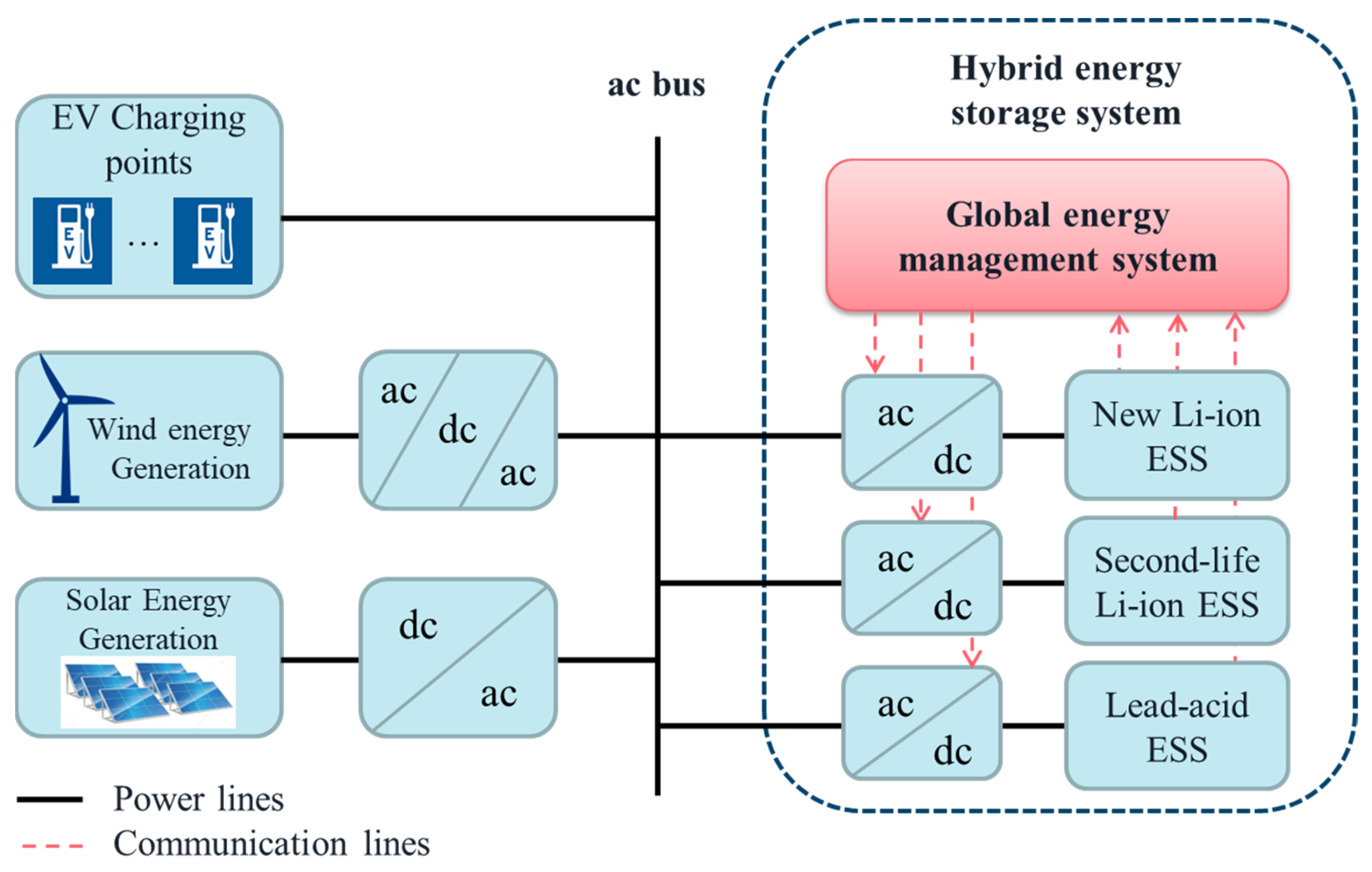
2.1.6. Autonomous Microgrid Model

As the MG modules were modelled separately, they may be configured into the entire MG model. Figure 2 shows the connections between different modules of the studied MG. The total renewable generation power, P r e n , is the sum of the WT generation power, P w t , and the solar generation power, P p v . From this, it is possible to calculate the difference between the renewable generation power and the EV demand power, P e v , as follows:
P e r , g e n ( t ) = P e v ( t ) P r e n ( t ) .
where P e r , g e n is the generation error power. When its value is positive, it means the generation is not enough, and its negative value implies more generation power than the EV demand power. Assuming the charging/discharging power of the HESS, P h e s s , one can write the instantaneous power balance of the MG as follows:
P e r , l o a d t = P e r , g e n t + P h e s s ( t ) ,
where P e r , l o a d is the load error power. A positive value of the P e r , l o a d means the EV demand power is not met, and a negative value of the P e r , l o a d means excess RES power is neither consumed by the EV load nor stored in the HESS. Note that P h e s s in (25) has positive values during discharging the HESS and negative values during charging the HESS. The HESS power, P h e s s , is the sum of the ESSs’ real powers obtained according to the global EMS calculations and the ESS models.
The HESS scheduled power and the generation error power, i.e., P h e s s , s c h and P e r , g e n , are the same values (See Figure 2). Nevertheless, the generation error power and its equivalent energy are the actual power and energy signals, but the HESS scheduled power and its equivalent energy are control signals which are used in the EMS. Note that the HESS scheduled energy and the generation error energy can be easily calculated by integrating P h e s s , s c h and P e r , g e n with respect to time. Some more details about the MG model signalling shown in Figure 2 can be found in [15].

2.2. Economic Modelling

Alongside the technical analysis and modelling of the charging station, this study also modelled the economic aspects of the system. There are several reasons for this approach. Firstly, as the objective of this work was to provide a design framework for an off-grid charging station that can be applied to a wide range of possible scenarios, for any proposed design of a system to be considered valid, it must be viable from both technical and economic perspectives. That is, the system must not only meet the technical requirements of the specified site, but it must also do so in a way that makes economic sense at the same site. Clearly, given the wide range of potential site ownership and operational configurations possible, it is not practical to give a single measure of economic viability. However, by considering the economic aspects of any proposed design it is possible to provide various metrics for that design, such as COE, payback period, etc., which can be used by the stakeholders of any given site to assess the economic viability of a proposed design, given their specific requirements.
A second key aspect of economic modelling is that of producing designs that are practical to construct in the real world. Whilst the technical models can produce designs which best meet the objectives of the site, they often result in systems that cannot be practically constructed due to the specification of equipment sizes or ratings that are not available commercially from suppliers. Using real-world data for equipment and other costings allows for the economic model to produce, as accurate as possible, an assessment of the cost of constructing and operating a given system. It is also used to feedback into the techno-economic model to ensure that any design produced is based on real components which are available for use in the system.
To this end, the economic analysis of the system is divided into categories covering each of the major components of the system. In this way, the economics of any one individual aspect can be isolated, and the methodology is also flexible enough to allow for the addition or removal of system components as required by the technical analysis. Note that the economic analysis does not cover any aspects relating to the land on which the site is located, as there is simply too much variation in land costs and acquisition options to present a meaningful analysis. The technical modelling does, however, give an overall area specification for the site, so this can be used along with local costings to arrive at an estimate of the land costs for the system at a given location.

2.2.1. Wind Generation Costs

Wind generation is modelled using the system topology as given in Section 2 and assumes that the turbines themselves include all the converter equipment to give a standard ac supply output. In this way, the economic model of each turbine is assumed as follows:
C t o t , w t = C p , w t + C i n s , w t + C r e p , w t + C o m , w t + C b r , w t .
Turbine costs are then further broken down into the initial capital costs of purchasing and installation (CAPEX costs), and operational and maintenance costs (OPEX). CAPEX costings cover the initial purchase, C p , w t , and installation, C i n s , w t , of the turbine equipment, together with forecasted replacement costs at the end of the turbine’s operational life, C r e p , w t . OPEX costings cover a yearly operation and maintenance budget, C o m , w t , along with blade replacement costs, C b r , w t , at intervals as specified by the manufacturer, e.g., seven years for a 6 kW wind turbine [33].

2.2.2. Solar Generation Costs

The economic modelling of the solar generation system is performed in a similar way to that of the wind generation by identifying the CAPEX and OPEX costs associated with the generation. In the case of solar, however, the analysis is somewhat more complex due to the more modular nature of the generation. Unlike the wind generation unit which consists of a single element containing all the generation equipment, the solar system is a collection of panels and inverters which, together, form the generation source. For this analysis, the modelling is based on basic units of 405 W ( = P r a t e d , p a n e l ) PV panels and 15 kW ( = P r a t e d , i n v ) solar inverters, and their purchasing costs can be calculated as follows:
C p a n e l s , p v = N p v × P r p a n e l ,
C i n v , p v = ( [ N p v × P r a t e d , p a n e l ( k W ) P r a t e d , i n v ( k W ) ] + 1 ) × P r i n v , p v ,
where P r p a n e l and P r i n v , p v are the unit price (GBP) of the PV panel and the inverter, respectively. An additional complication arises from the fact that the panels themselves require additional infrastructure for their operation. As multiple panels supply one inverter, and the inverters are generally physically distant from the panels, there is a wiring cost associated with connecting each panel to the system. The panels also need to be supported mechanically to ensure they are appropriately oriented to achieve maximum generation; again, this adds a structural cost to each panel. The economic model accounts for these balance of system (BOS) costs and considers the electrical, C e b o s , p v , and structural, C s b o s , p v , costings separately. Another term is also assumed as overhead costs, C o h , p v , to cover any other initial costs not categorized in previous terms. All these costs are modeled as follows:
C e b o s , p v = N p v × P r e b o s , p a n e l ,
C s b o s , p v = N p v × P r s b o s , p a n e l ,
C o h , p v = N p v × P r a t e d , p a n e l × P r o h , p v ,
where P r e b o s , p a n e l , P r s b o s , p a n e l , and P r a t e d , p a n e l are unit prices of electrical BOS in GBP/panel, structural BOS in GBP/panel, and overhead costs in GBP/kW, respectively. The final term of the CAPEX costs is replacement costs, C r e p , p v , assumed as 1.2 times the purchasing costs as a total replacement cost prediction after the PV lifetime. On the other hand, the OPEX costs are considered as follows:
C o m , p v = N p v × Y t o t × P r o m , p a n e l ,
where Y t o t is the total years under study in the planning, and P r o m , p a n e l is the operation and maintenance costs of each panel in GBP/year. Therefore, the total solar generation unit costs can be calculated as follows:
C t o t , p v = C p a n e l s , p v + C i n v , p v + C e b o s , p v + C s b o s , p v + C o h , p v + C r e p , p v + C o m , p v

2.2.3. EV Charging Station Costs

For this analysis, 7 kW ac chargers are assumed for the EV charging station. As self-contained units, the costings associated with this are taken to be simply the purchase costs of the chargers themselves, indicated by C c h a r g e r , e v .

2.2.4. ESS Costs

As described in the previous section, the design chosen for the ESS is of a hybrid type comprising three separate storage systems. For the economic model, costs are obtained for purchasing each of the three storage elements, C p u r , e s s , together with the associated electrical component costs, i.e., the electrical BOS, C e b o s , e s s , and installation costs, C i n s , e s s . Costings are also sourced for the bidirectional inverters required for each storage type, C i n v , e s s , together with the associated electrical cabinet and switchgear costs, C c a b , e s s . Given the relatively complex nature of the ESS, with the need to manage the power flow through the separate types of storage, a cost is included for control equipment and IT infrastructure associated with the ESS energy management system in C e b o s , e s s . The costs are calculated for each ESS as follows:
C p u r , e s s = E n o m , e s s × P r k W h , e s s ,
C i n s , e s s = E n o m , e s s × P r k W h , i n s ,
C i n v , e s s = ( [ C r a t e , m a x × E n o m , e s s P r a t e d , i n v ] + 1 ) × P r i n v , e s s ,
C c a b , e s s = [ E n o m , e s s E n o m , c a b ] × P r c a b , e s s ,
where P r k W h , e s s , P r k W h , i n s , P r i n v , e s s , and P r c a b , e s s are the unit prices for purchasing the energy storage per kWh (GBP/kWh), its installation per kWh (GBP/kWh), purchasing each inverter, and purchasing each cabinet, respectively. P r a t e d , i n v is the rated power of the inverter, and E n o m , c a b is the nominal capacity of the cabinet. Note that C e b o s , e s s is assumed as a constant cost for each ESS. The replacement cost of the ESS, C r e p , e s s , is considered to be the same as the purchasing cost, i.e., C p u r , e s s . The costs of the container, C c o n , h e s s , in which to house all the ESSs, is also considered for the HESS according to required volume of the ESS and enough room for operation and maintenance.
The estimated costs for energy storage systems vary quite widely depending on the source, and, often, the quoted price per kWh for battery technologies is based on the price of the cells alone without any of the additional hardware required to make those cells into a practical ESS. For this study, quotes were obtained for plug-and-play ESSs of the types required, which include not only the storage elements but also the associated battery management systems (BMSs), enclosures, contactors, etc., required for a working system. As with the previous elements, costings for each storage technology are modelled separately, allowing for the model to easily handle the number or types of storage being changed. Therefore, the total costs of a HESS including N number of ESSs, C h e s s , is calculated as follows:
C h e s s = i = 1 N ( C p u r , e s s i + C i n s , e s s i + C i n v , e s s i + C c a b , e s s i + C e b o s , e s s i + C r e p , e s s i ) + C c o n , h e s s .

2.2.5. Construction Costs

Aside from the costs associated with the physical equipment required, establishing the charging station will also incur additional costs associated with preparing the site. These construction, design, and management (CDM) costs cover a wide range of activities including planning and permit approval from the local authorities, site access, groundworks, contractor accommodation, health and safety compliance, etc.
Given the broad area covered, the specific CDM costing for any given site is highly variable and extremely difficult to predict in advance. It is, however, likely to be a significant proportion of the total costs and, therefore, should be accounted for in the economic modelling. To this end, the estimated CDM cost, C c d m , (GBP) is included in the model, with the value being taken from the authors’ recent experiences with projects similar in scope to that investigated here [34].

2.2.6. Total Costs

The total costs for the proposed system are given in (38) by taking the sum of the costings for each individual element, accounting for the projected lifetime of the system. The total cost is used to inform the overall economic viability of the proposed design, and it feeds into the overall present-value analysis of the system.
C T , m g = C t o t , w t + C t o t , p v + C c h a r g e r , e v + C h e s s + C c d m .

3. Microgrid Planning

Firstly, a planning characteristic is developed according to COE. Then, the sensitivity analysis method is explained, which is used to compare feasible plans according to the planning characteristics. Two sensitivity analysis algorithms are used to investigate two different combinations of changeable parameters, for example, one studies a simple single ESS in the system, and the second one investigates a HESS.

3.1. Proposed MCOE as a Planning Characteristic

There are a lot of economic, technical, and techno-economic characteristics to be considered as MG planning indices, such as total cost, net present cost, EV unmet energy (UME), and COE. Although all these characteristics are important in a sizing/planning study to consider different aspects of the MG design and implementation, a comprehensive characteristic or a smaller group of these characteristics is required to make a decision about the best plans for the MG. Here, a modified COE is proposed, namely, the MCOE, in which the original COE is strengthened for techno-economic planning by adding two important technical features. The first feature is the HESS present value, which calculates the total value of all ESSs used in the HESS after the nominal operating period of the MG. The present value of i-th ESS is given as follows:
E S S i   p r e s e n t   v a l u e = ( S O H i E O L i / 100 ) × E n o m × P r e s s , i ,
where S O H i = ( E n o m , d e g / E n o m ) × 100 . The second feature is the UME penalty, which can be assumed as a virtual cost as:
U M E   p e n a l t y = W u m e k W h × C t a r i f f ( £ / k W h ) ,
where W u m e is the EV unmet energy calculated by integrating the positive values of the load error with respect to time, i.e., W u m e = P e r , l o a d + ( t ) d t . Therefore, the MCOE (GBP/kWh) is proposed as follows:
M C O E = C T , m g i E S S i p r e s e n t   v a l u e + U M E   p e n a l t y   E V   m e t   e n e r g y ( k W h ) .
where the EV met energy is the total energy provided either directly by renewable energies or by discharging the HESS, which can be calculated from the corresponding EV met power, P e v , m e t ( t ) , as follows:
P e v , m e t ( t ) = ( P r e n ( t ) + P h e s s + ( t ) ) , P e r , g e n ( t ) > 0 P e v ( t ) , P e r , g e n ( t ) 0
E V   m e t   e n e r g y = P e v , m e t ( t ) d t .
Note that assuming the present value of the ESSs in the MCOE results in a degree of freedom in selecting the study years, which is especially less than the ESS lifetime. It makes the planning studies flexible because the input data for renewable generations and the EV demand may not always be available with good precision for any number of years. On the other hand, although the EV met energy is presented in the original COE to reflect this technical aspect, with the economic feature of total cost in decision-making, the UME penalty increases the share of technical features to consider a greater safety margin in the planning process.
In addition to the MCOE, the original economic and technical characteristics are used in the planning studies, e.g., total costs, EV met energy percentage, and COE. The COE can be easily calculated using (42) without considering the two added terms, and the EV met energy percentage can be calculated using (44) as follows:
E V   m e t   e n e r g y   p e r c e n t a g e = E V   m e t   e n e r g y ( k W h ) E V   e n e r g y   d e m a n d ( k W h ) × 100 ,
where E V   e n e r g y   d e m a n d k W h = P e v ( t ) d t .

3.2. Sensitivity Analysis-Based Planning

To find the RES and ESS sizes according to techno-economic characteristics introduced in Section 3.1, two sensitivity analysis-based planning (SAP) scenarios are investigated. In the first one, namely, SAP1, the techno-economic sizes of the wind generation unit, solar generation unit, and a single ESS are obtained while the single ESS can be each one of the studied technologies. In the second planning scenario, namely, SAP2, the techno-economic sizes are obtained simultaneously for all ESS technologies of the HESS while the wind and solar generation units’ sizes are assumed fixed based on the SAP1 results.

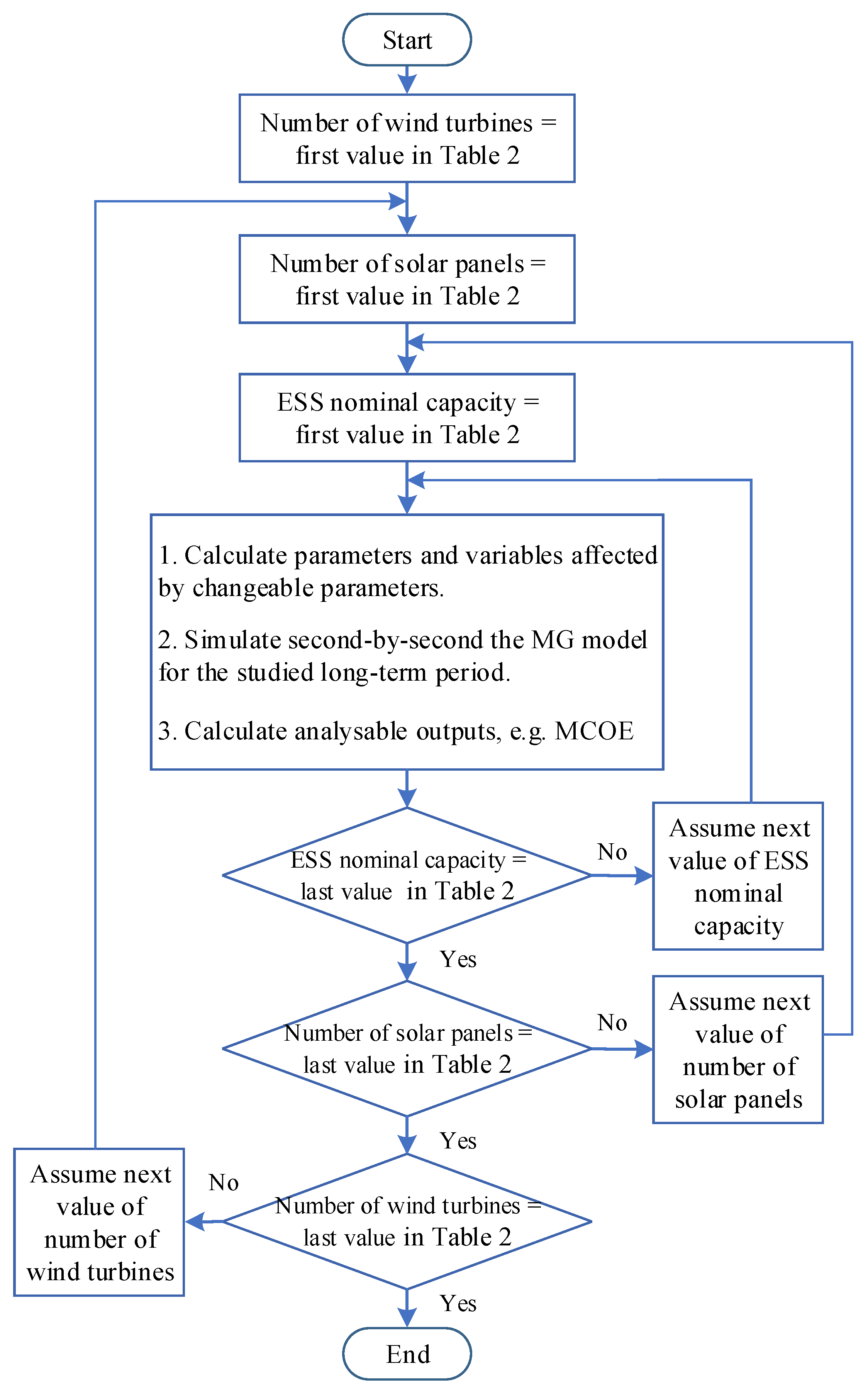
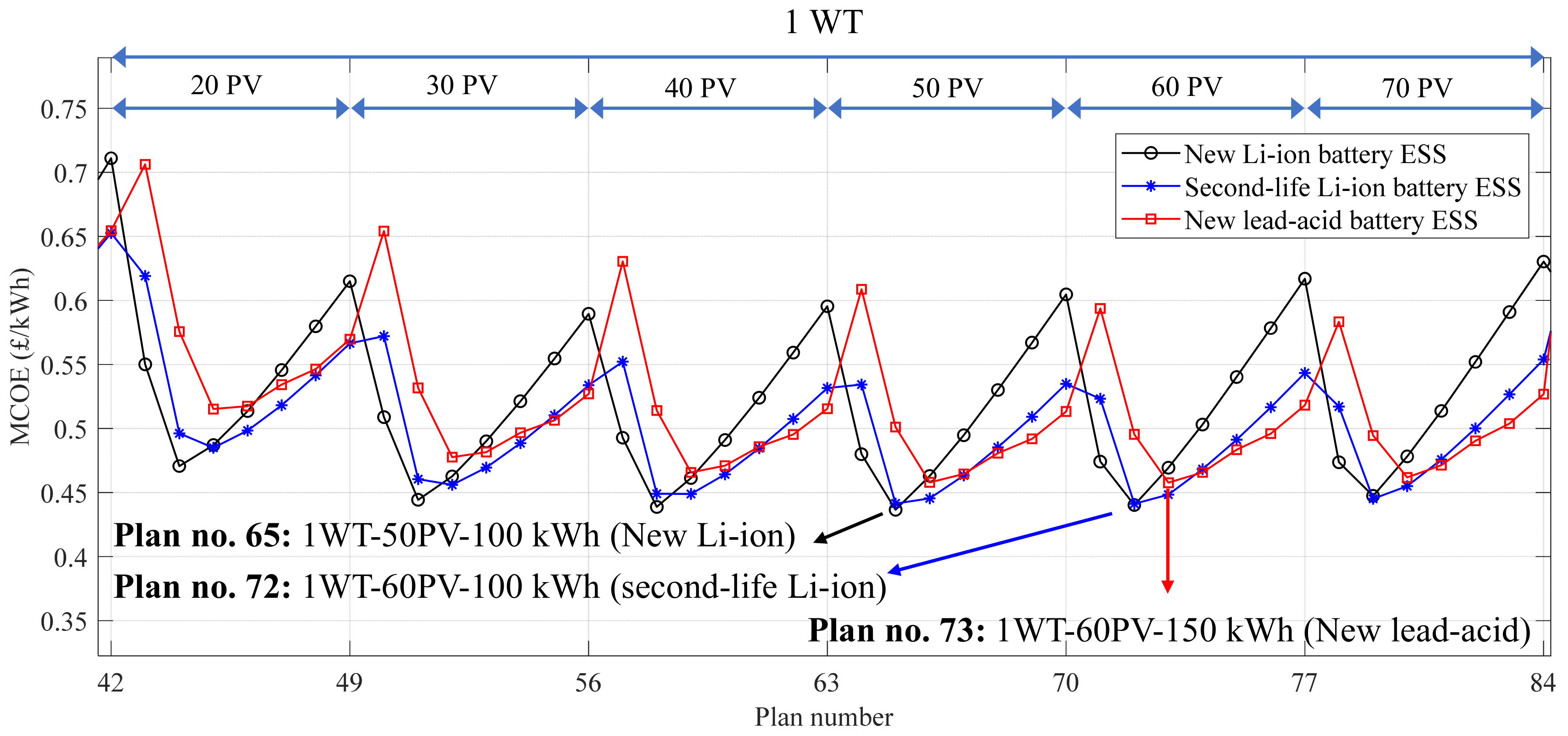
3.2.1. Wind Generation, Solar Generation, and Single ESS Planning (SAP1)

Figure 5 shows a flowchart of SAP1 for the simultaneous sizing of wind generation, solar generation, and a single ESS. The number of wind turbines, the number of solar panels, and the ESS nominal capacity are the changeable parameters of SAP1, and their possible values are represented in Table 2. The ranges were selected based on some preliminary studies to ensure that the combination of the RESs and the ESS could provide reasonable energy values for the EV charging station demand, on the one hand, as well as to satisfy the feasibility of the targeted location, on the other hand. These preliminary studies cannot be presented here due to the limited space of the paper. Each wind turbine had a 6 kW rated power with a 20 m hub height, which is a suitably small wind turbine for installation near a car park, which is a busy place. The solar panels had ratings of 405 W, 1.95 m2, and 20% efficiency, and their maximum number is also limited by the available area for the installation of the EV charging station.
The wind speed and solar radiation data were obtained for 2013–2022. Each one of the ESS technologies presented in Table 1 is assumed as a single ESS. The EV demand was predicted for 10 years using the predicted total and electric car populations for 2022–2031 [35]. After calculating the parameters and variables affected by changeable parameters for each combination of the number of wind turbines, number of solar panels, and ESS nominal capacity, the MG model was simulated second-by-second for the studied 10 years. It is noteworthy to mention that the steps in the number of solar panels and the ESS nominal capacity should neither be very small, which causes numerous simulations and very long simulation times, nor very large, which leads to being away from the ideal optimal plan.
The simulation results include some analysable outputs, e.g., the EV met load, and the MCOE, which can be compared for different plans, i.e., the MG model for different combinations of the changeable parameters.

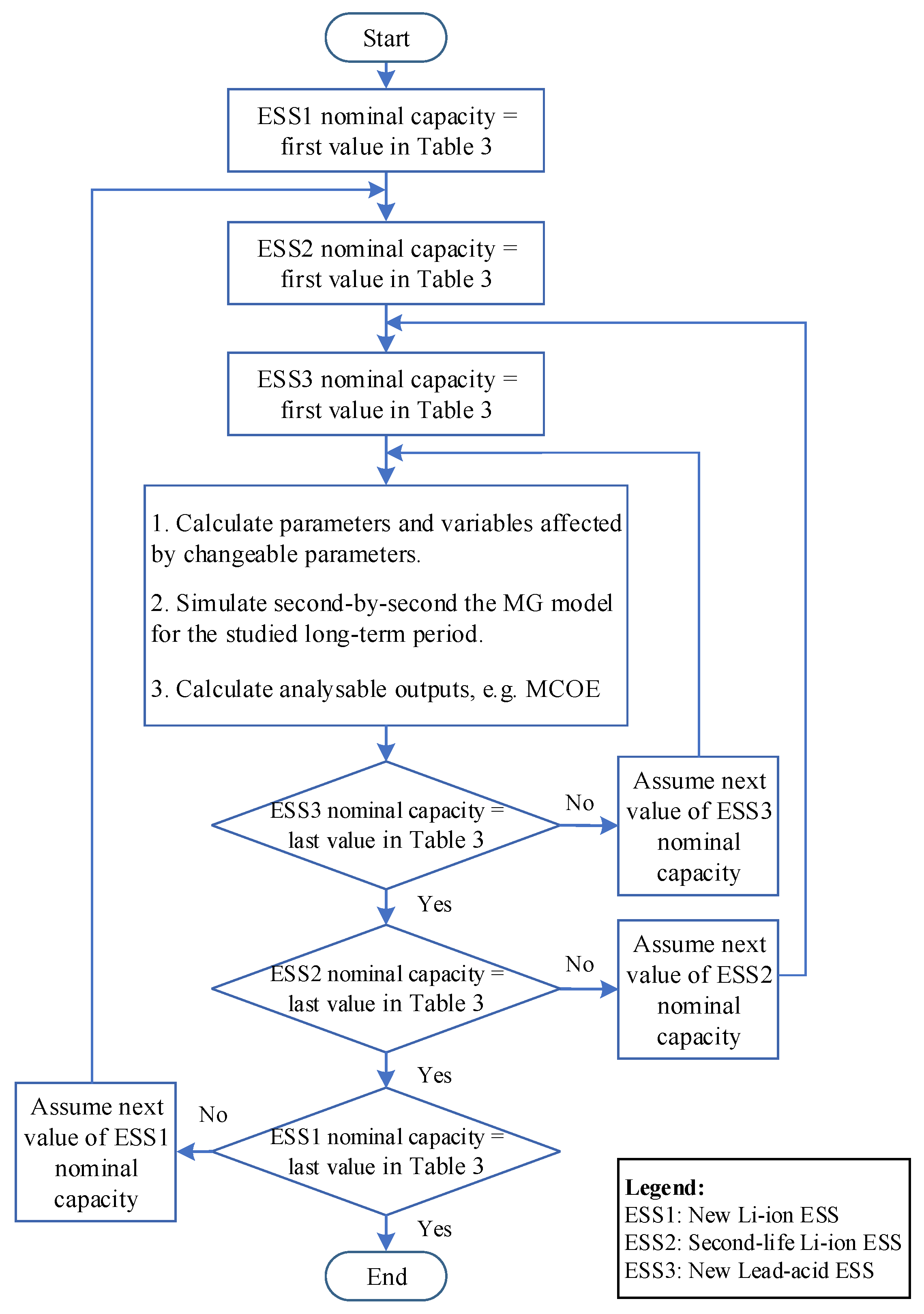
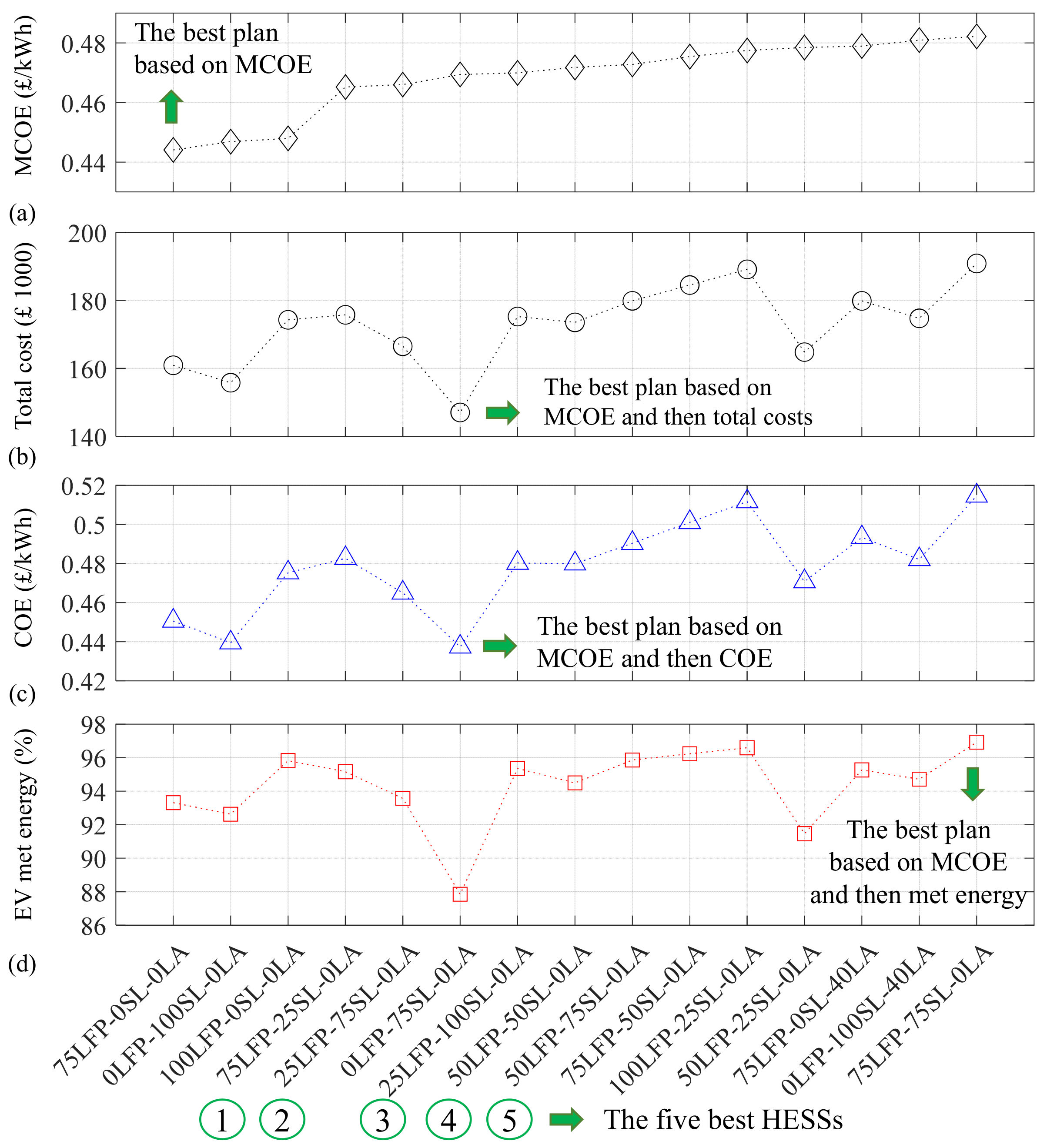
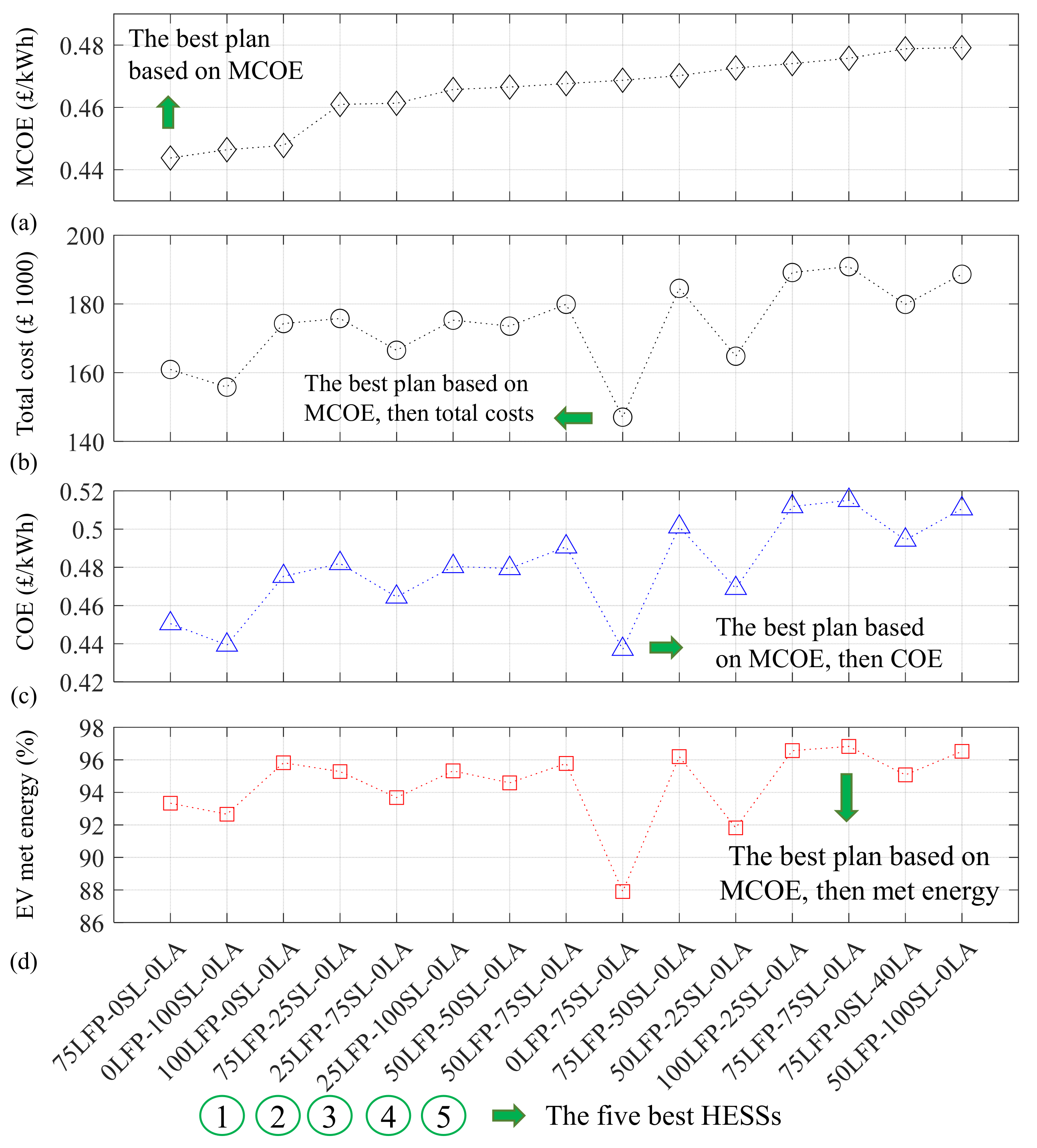
3.2.2. Hybrid ESS Planning (SAP2)

Figure 6 shows a flowchart of SAP2 for the simultaneous sizing of different ESS technologies in the HESS. The nominal capacities of the new Li-ion, the second-life Li-ion, and the new lead–acid battery ESSs are considered the changeable parameters of SAP2, and their feasible values are shown in Table 3. A zero value means removing the relevant ESS from the HESS. One wind turbine and 60 solar panels of the types presented in SAP1 are assumed as fixed numbers here. This decision is according to the SAP1 results, which are explained in Section 4.2 and Section 4.3.1. The EV demand is the same as SAP1. The characteristics of the ESS technologies are found in Table 1. After calculating the parameters and variables affected by changeable parameters for each combination of the nominal capacities of the three ESS technologies, the MG model was simulated second-by-second for the studied years. The simulation outputs are compared for different plans to find the best HESSs.

4. Simulation Results and Discussions

4.1. Studied System

The main structure of the studied system is shown in Figure 1, including the EV charging station, a wind generation unit, a solar generation unit, and the HESS (a single ESS in some studies), which is modelled in Figure 2 and Section 2 through technical and economic modelling. The technical parameters and inputs are already presented in Section 2 and Section 3. Unit prices and costs used in the simulations are presented in Table 4. All the results were obtained for the sensitivity analysis-based planning scenarios known as SAP1 and SAP2. The simulations were executed in a combined environment of Editor and Simulink in MATLAB 2022b (https://www.mathworks.com/, accessed on 15 January 2024). The iterative process of the sensitivity analysis-based planning algorithms shown in Figure 5 and Figure 6 was implemented in Editor using three cascaded for loops. The pre-simulation calculation of the parameters and variables affected by the changeable parameters and post-simulation calculation of the analysable outputs, respectively, shown in items 1 and 3 in the flowcharts, were also performed in Editor using appropriate coding of the input parameters and corresponding formulas. The MG simulation, shown in item 2 in the flowcharts, was performed in Simulink using only Simulink library tools. Appropriate codes/blocks were used to connect these two environments of MATLAB, e.g., sim to simulate a Simulink model in Editor and the To Workspace block to make Simulink outputs available in Editor.
A discrete solver with a fixed-step sample time of 10 min was used in Simulink to simulate the studied MG for each ten-year plan. The simulations were performed on a PC with a 3.0 GHz Intel(R) Core (TM) i5-8500 CPU and 8 GB RAM.

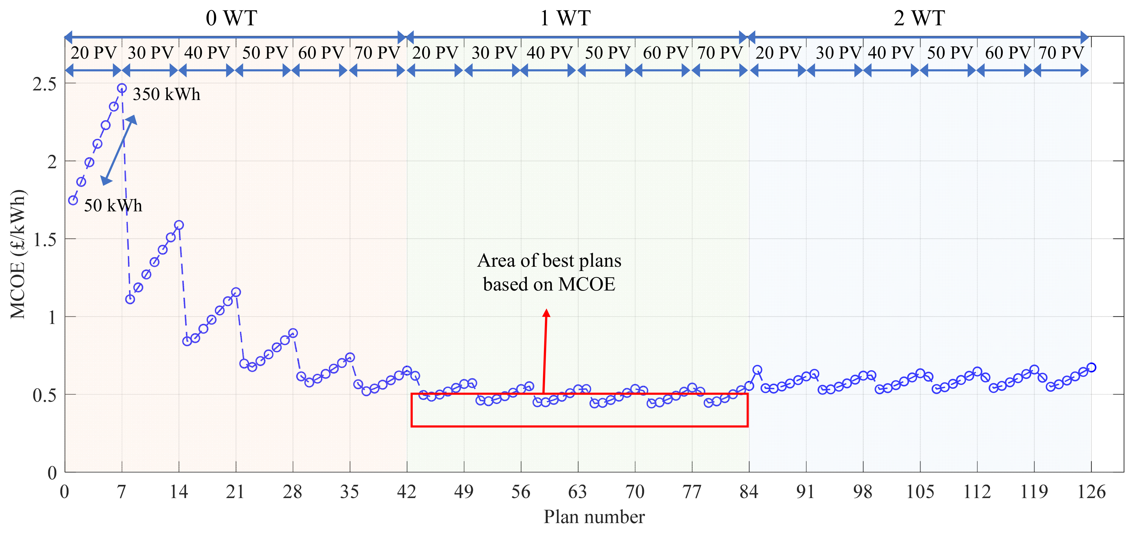
4.2. Comparing All Feasible Plans in SAP1

The impact of changing the number of wind turbines and solar panels as well as the nominal capacity of the single ESS on the decision-making characteristics was worth investigating in SAP1, where the techno-economic sizes of the renewable energy resources and an ESS should be obtained. This was performed for when the single ESS is the second-life Li-ion battery ESS and the proposed MCOE were considered as the decision-making characteristic. The results are shown in Figure 7, where each circle shows a plan, e.g., in plan number 14, no wind turbine and only 30 PV panels are used, and the ESS nominal capacity is 350 kWh. The dashed line is used to follow the changes on the MCOE more easily. The results show the area of the best plans, including one wind turbine, any number of solar panels, and the lower values of the second-life Li-ion battery ESS capacity. To select the best plans, more details are required; therefore, other technical/economic characteristics are added into the analysis, as presented in the next scenarios.

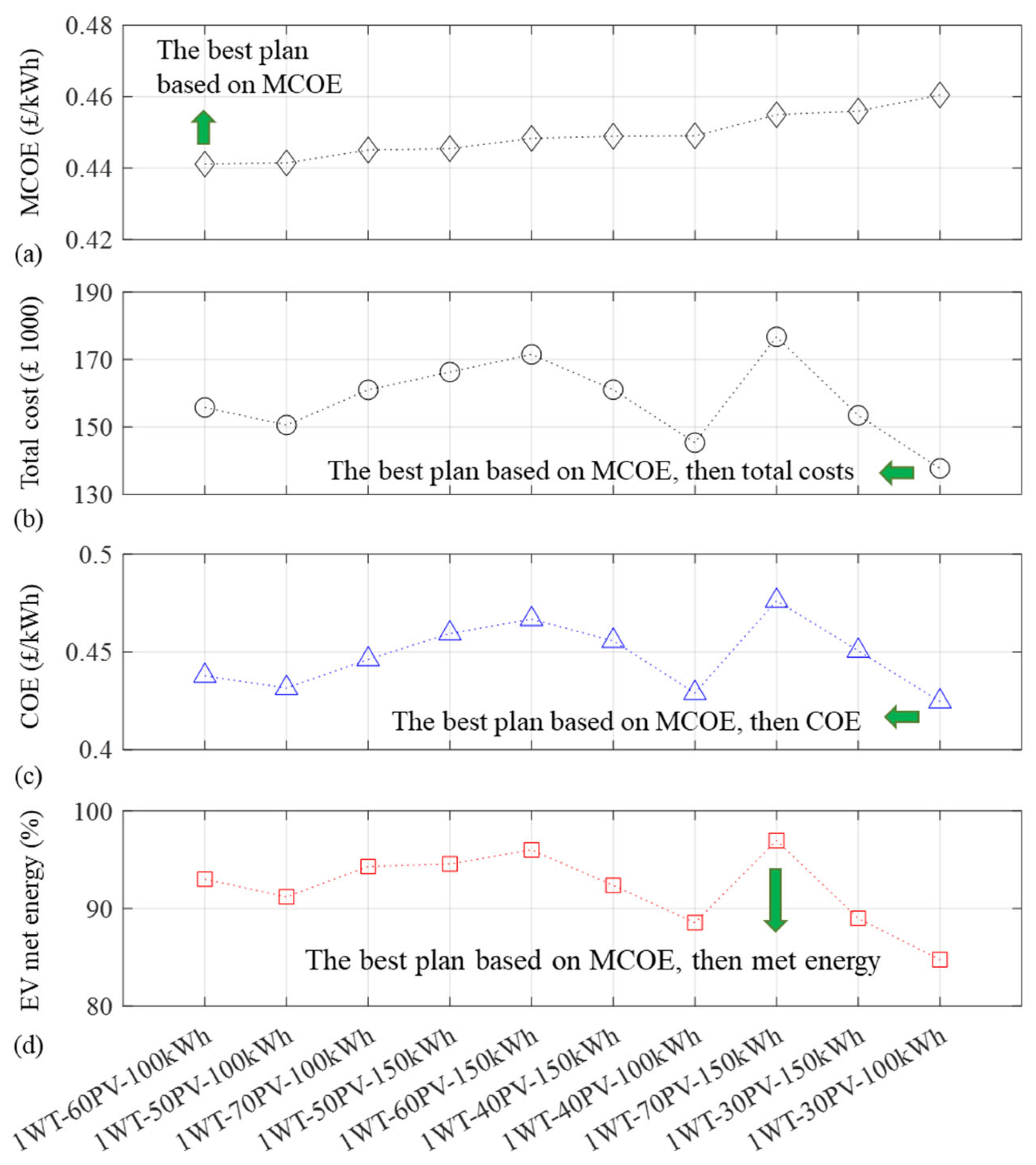
4.3. Techno-Economic Comparison of Best Plans in SAP1

4.3.1. Ten Best Plans in SAP1

The ten best plans from Figure 7, discussed in the previous section, are selected according to their MCOE, which are shown in Figure 8a. The horizontal axis shows the number of wind turbines, the number of solar panels, and the ESS nominal capacity of the plans in the form of the number of wind turbine, WT, number of solar panels, PV, and nominal ESS capacity, kWh. Therefore, all ten best plans based on MCOE require only one wind turbine, and the best plan needs one wind turbine (6.2 kW), 60 solar panels (each one being 405 W, 20%), and 100 kWh as the nominal capacity of the second-life Li-ion battery ESS. Figure 8b shows the total cost of the ten best plans based on the MCOE, where there are some other plans with a lower total cost than the best plan based on the MCOE. One can select 1WT-30PV-100kWh as the best plan based on the MCOE and total costs. As shown in Figure 8c, this plan is also the best plan based on the COE after sorting the best plans based on the MCOE. However, this plan has about 85% EV met energy as shown in Figure 8d, which is a low value in comparison with the best plan based on the MCOE, which has 93% met energy. Nevertheless, there is another best plan based on the criteria of the MCOE and the EV met energy with the highest met energy. It includes one wind turbine, 70 solar panels, and the ESS with a 150 kWh nominal capacity, which yields about 97% EV met energy. Therefore, there are different options to selected as the best plan, which should be constrained by real limitations in different aspects.

4.3.2. Comparing Different Single ESS Technologies in SAP1

The same studies in Section 4.2 and Section 4.3.1 are performed for the other two ESS technologies, i.e., the new Li-ion and the new lead–acid battery ESSs, with all other conditions of the wind turbines, the solar panels, and the EV energy demand being kept without any changes. The area of best plans based on the MCOE is the same for all three ESS technologies, which implies using one wind turbine. Therefore, this area is shown in Figure 9, where all three ESSs can be compared for a different number of solar panels and different values of ESS capacities. The best plans based on the MCOE are shown in Figure 9, which are also represented in Table 5 for all single ESS technologies under the study. By selecting the new Li-ion battery ESS, a nominal capacity of 100 kWh, one wind turbine, and 50 solar panels are required to provide 94.6% EV met energy and 86.4% SOH. Although selecting the second-life Li-ion battery needs 10 more solar panels and results in 93% met energy and 68.9% SOH, the corresponding plan is cheaper by about GBP14,000, and it has a lower COE. Note that the SOH decrease of both the new and second-life batteries is approximately in the same range. The total costs of the new Li-ion and the new lead–acid battery ESS technologies are nearly the same. However, the MCOE, the COE, and the met energy of the new Li-ion battery ESSs are better than the equivalent amounts of the new lead–acid battery ESS. Moreover, the new lead–acid battery ESS requires a replacement. Therefore, both the new and second-life battery ESSs are more suitable choices than the new lead–acid battery ESS. Furthermore, the second-life battery ESS is the most cost-effective choice and can satisfy the technical requirements well.

4.4. Techno-Economic Comparison of Best Plans in SAP2

In SAP2, the HESS can be managed by both the priority-based EMS and the power-sharing-based EMS. Here, these EMSs are studied separately to compare their performance in the MG planning studies as well as to compare their technical performance, e.g., their SOH.

4.4.1. Best Plans Using the Priority-Based EMS

Figure 10 shows fifteen best plans obtained in SAP2, including HESS plans and using the priority-based EMS based on the MCOE. The horizontal axis shows the plans by their HESS capacity, where the first value is the nominal capacity of the new Li-ion battery ESS, where LFP is an abbreviated equivalent for Lithium Iron Phosphate as the type of the Li-ion battery ESS used in the studies; the second value shows the nominal capacity of the second-life battery ESS, where SL is an acronym for the second-life Li-ion battery ESS; the third value indicates the nominal capacity of the new lead–acid battery ESS, and LA is an acronym for this ESS.
The MCOE shown in Figure 10a changes in a low range, from GBP 0.44/kWh to about GBP 0.47/kWh, for all fifteen plans. The best plan based on the MCOE includes only the new Li-ion battery ESS with a 75 kWh nominal capacity. Figure 10b,c show the total cost and the COE of the best plans, where the best plan based on these two features is another single ESS including only the second-life Li-ion battery ESS with a 75 kWh nominal capacity. The MCOE, COE, and total costs, as the techno-economic and pure economic characteristics, show the suitability of single-ESS plans, e.g., 75LFP-0SL-0LA and 0LFP-75SL-0LA, with respect to the HESS-included plans. The five best HESS plans are indicated by numbers in circles, where they are generally more expensive than the best single-ESS plans. However, they have higher EV met energy percentages. After sorting plans based on the MCOE, the best plan based on the EV met energy is a HESS including both the new and second-life Li-ion battery ESSs with the same nominal capacities of 75 kWh (see Figure 10d). This plan provides an EV met energy of about 97%, which shows a high availability of the RESs and ESSs. Nevertheless, the new law of the UK government about charging points require the provision of 99% reliability/availability during each calendar year [41], which will be a challenge for a future work.

4.4.2. Best Plans Using the Power Sharing-Based EMS

Figure 11 shows fifteen best plans obtained in SAP2 including HESS plans and using the power-sharing-based EMS, based on the MCOE. The techno-economic results are similar to those of the priority-based EMS shown in Figure 10. The best plans based on the MCOE, total costs, and the COE are single-ESS plans as shown in Figure 11a–c. However, similar to the results of priority-based EMS, the best plan based on the EV met energy, after sorting plans according to the MCOE, is a HESS including a 75 kWh of each new and second-life battery ESS (see Figure 10d and Figure 11d). The five best HESSs based on the MCOE are also the same as those obtained using the priority-based EMS. Therefore, the studied EMS strategies do not have a considerable impact on the techno-economic planning results. Nevertheless, the next subsection compares these two EMS strategies in more detail, emphasizing their SOH.
Note that the plans including the new lead–acid battery EMS are not favourable, either from technical aspects, or in terms of being cost-effective. Their faster ageing when compared to the Li-ion battery ESS, and, consequently, their replacement, at least once for a ten-year lifetime, are the main reasons. Furthermore, the majority of the best plans include only two types of ESS technologies, which is due to adding the required infrastructure for each ESS, e.g., an independent inverter for each ESS.

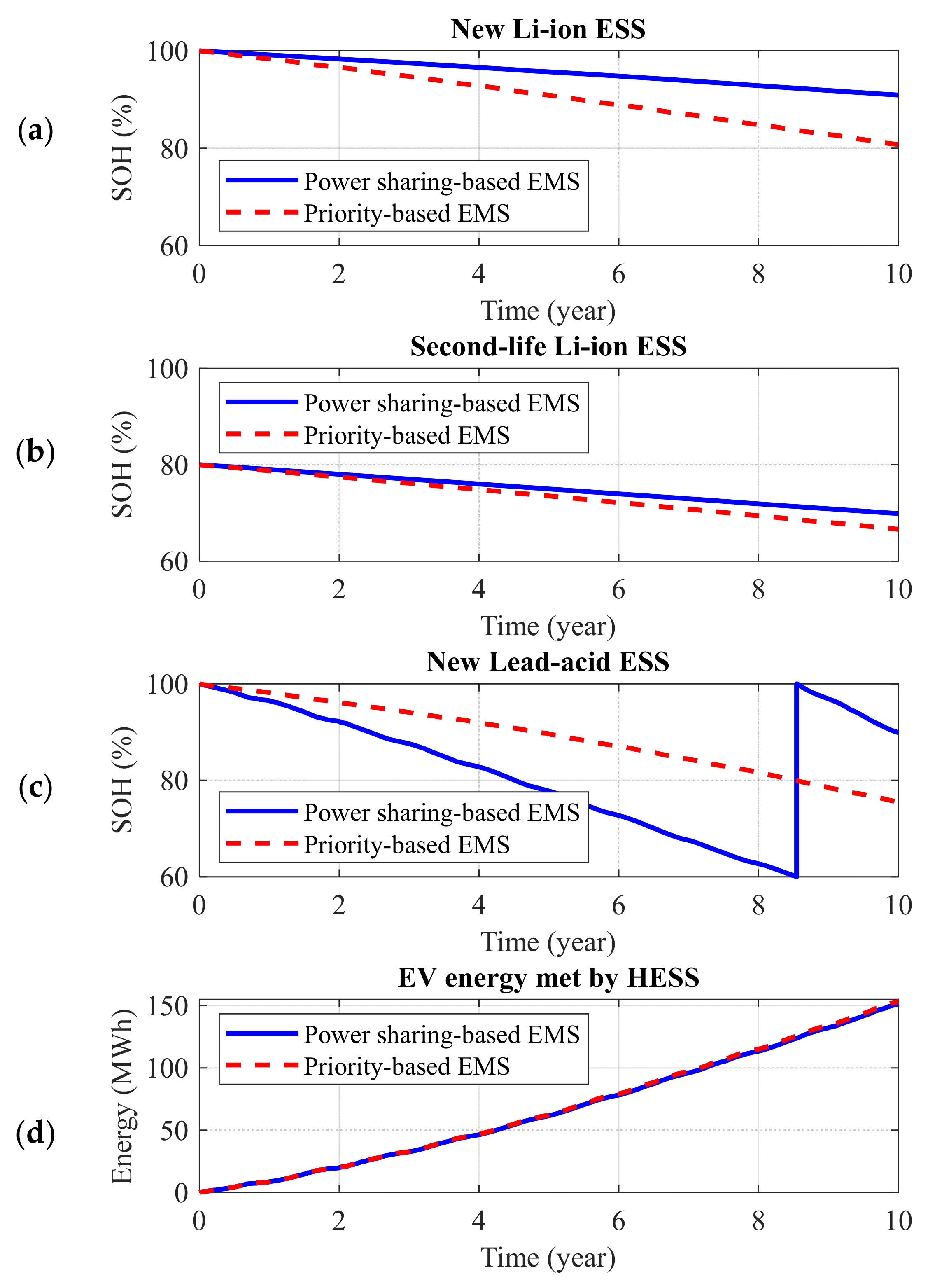
4.4.3. Comparing EMS Strategies for Best HESS Plans

Figure 12 shows a comparison of the priority-based and power-sharing-based EMSs for a HESS including a 50 kWh new Li-ion, a 50 kWh second-life Li-ion, and a 50 kWh new lead–acid ESS. Other simulation requirements, i.e., MG structure and information, are those used in SAP2 studies. Figure 12a–c show the SOH of the ESS technologies, where the power-sharing-based EMS leads to higher SOHs for both new and second-life ESSs than the priority-based EMS after ten years. However, the new lead–acid ESS needs one replacement in the ninth year when using the power-sharing-based EMS, while this is not required when using the priority-based EMS due to the very low usage of the third priority, i.e., the lead–acid ESS. According to Figure 12d, the EV met energy provided by the HESS is approximately the same for both EMS strategies. Therefore, to complete a comparison of the EMSs, some other characteristics need to be investigated.
Table 6 shows a comparison of the best plans of HESS in SAP2 for both EMS strategies including the MCOE, the COE, the EV met energy, and the SOH of the ESSs. As discussed generally in Section 4.4.2, and as illustrated in Table 6, the most important MG planning features like the MCOE, the COE, and the EV met energy are not affected considerably by changing the EMS strategy for each plan. In fact, the difference in MCOE and COE values is <GBP 0.01/kWh, and the EV met energy difference is around 0.1%. Moreover, total costs, which are not shown in Table 6, are the same for both EMSs due to the absence of replacements. Nevertheless, by focusing on the HESS SOH column, a remarkable improvement in the ESS SOHs can be seen for all plans when the power-sharing-based EMS is used. Therefore, the power-sharing-based EMS can improve the HESS SOH, but it does not have a considerable impact on the techno-economic characteristics of the MG planning.

4.4.4. Multi-Objective Decision-Making Constrained by Total Costs

Single and multi-objective decision-making are presented for single/hybrid ESSs in Section 4.4.1 and Section 4.4.2 by sorting SAP2 plans based on the MCOE and then searching for the best plans according to total costs, the COE, and the EV met energy. On the one hand, the MCOE is a powerful techno-economic characteristic including the COE benefits in MG planning studies and more benefits due to its added terms. On the other hand, pure economic and technical characteristics such as the total costs and the met energy are still important for MG designers due to their straightforward and easily analysable information for decision-making. Therefore, multi-objective decision-making assuming all these three characteristics, i.e., the MCOE, total costs, and the EV met energy, can be of high interest. Figure 13 shows the MCOE (blue circles) and EV met energy (red stars) of all plans in SAP2 employing the power sharing-based EMS, while total costs are restricted in a range of values by designers. This range is also selected to include the minimum values of the MCOE, which results in holding the EV met energy higher than 90%. Table 7 shows the best single/hybrid ESS plans when assuming that the total costs range between GBP160,000 and GBP180,000 and that the MCOE is less than GBP 0.5/kWh. Therefore, a wide range of plans are provided, including suitable values of the MCOE and the EV met energy as well as reasonable amounts of total costs based on the designers’ decision. Moreover, since the power-sharing-based EMS is used, the SOHs of ESS technologies show high values without any replacements during the 10-year study period.

4.5. Limitations and Future Work Potentials

Due to both the project and paper limitations, some valuable studies and analyses could not be performed, and they are listed below for future works.
  • Uncertainty analysis for the inputs of the model like renewable energies and EV charging station parameters can be performed to study the impact of uncertainties on the planning results.
  • Standard requirements for EV charging station availability can be considered as a necessary minimum EV met energy percentage, which is now 99% in the UK [41]. Therefore, the best plans can be found according to the MCOE and other introduced features assuming this constraint.
  • Different combinations of existing ESS technologies can be considered to improve the technical features of the HESS and overall MG, e.g., less overall HESS capacity fade, less EV unmet energy demand, and higher energy density. Soluble lead flow batteries can be hybridized with lead–acid and Li-ion batteries.
  • Global energy management for HESS plays an important role in ESSs’ SOH and an indirect role in planning features like total costs and cost of energy. Different methods of global energy management can be compared to study their impact on both HESS and MG features and select the best ones.
  • Due to the intermittency of renewable energies as the only sources of energy for off-grid EV charging station MGs, it would be valuable to study seasonal long-term storages, e.g., hydrogen storage systems.
  • Since ESS technologies and EV charging station infrastructures develop very fast nowadays, considering potential technological advancements in modelling, it would be a good idea to investigate, especially, their impact on economic modelling.

5. Conclusions

In this paper, the techno-economic planning of a fully renewable energy-based electric vehicle charging station as an isolated microgrid (MG) is presented. Technical and economic modelling of all MG components are provided, where an enhanced power-in-power-out model of energy storage systems (ESSs) is presented, which is suitable for long-term studies, e.g., the planning and sizing of hybrid ESSs and MGs. This model can be generalized for a considerable number of electrical and electro-chemical energy storage technologies without any structural modification. A modified cost of energy (MCOE) is proposed as a new techno-economic characteristic for MG planning, which reflects the ESS values and the unmet energy penalty to the normal cost of energy in long-term studies. The MCOE provides a more comprehensive characteristic than other technical, economic, and techno-economic characteristics for decision-making alone. Using it for evaluating the plans in a sensitivity analysis-based planning resulted in a wide range of sorted plans for comparison. As the second criterion in double-objective decision-making, the total costs of the MG construction, cost of energy, and total met energy were used to provide more understandable values to compare plans. In the single ESS sensitivity analysis studies, the required number of wind turbines and solar panels, and the required capacity of a single ESS, were changed to find the best plans satisfying the demand for the electric vehicle charging station constrained by economic limitations. In the hybrid ESS studies, the best nominal capacities of different ESS technologies were obtained through multi-objective decision-making according to the MCOE, total costs, and met energy. Although the proposed power-sharing-based energy management system does not have a considerable impact on the techno-economic features of the best plans, it improves the state of health of some ESS technologies. However, future work will fully focus on the impact of more types of global energy management systems in hybrid ESSs on the sizing and planning characteristics.

Author Contributions

The authors confirm their contribution to the paper as follows: conceptualization: M.N. and D.A.S.; modelling and simulation: M.N., D.P. and Y.A.-W.; data collection: E.F. and A.C.; discussion, analysis, and interpretation of results: M.N., M.J.S., E.E.F.B., D.A.S., M.P.F. and D.T.G.; draft manuscript preparation: M.N., D.P., M.J.S., A.K. and Y.A.-W.; editing and review: M.N., E.E.F.B., D.A.S., M.P.F., D.T.G. and A.C. All authors have read and agreed to the published version of the manuscript.

Funding

This research was funded by the Engineering and Physical Sciences Research Council (EPSRC) through the ‘Future Electric Vehicle Energy Networks supporting Renewables (FEVER)’ grant number EP/W005883/1 and the APC was funded by the University of Southampton.

Data Availability Statement

Restrictions apply to the availability of the car park data. It is obtained from a third party, where sharing is not allowed.

Conflicts of Interest

The authors declare no conflict of interest.

Nomenclature

Abbreviations
BMSBattery management system
BOSBalance of system
CAPEXCapital costs (GBP)
CDMConstruction, design, and management
COECost of energy (GBP/kWh)
DODDepth of discharge
EMSEnergy management system
ESSEnergy storage system
EVElectric vehicle
FEVERFuture electric vehicle energy networks supporting renewables
HESSHybrid energy storage system
ITInformation technology
LALead acid
Li-ionLithium-ion
MCOEModified cost of energy (GBP/kWh)
MGMicrogrid
OPEXOperational and maintenance costs
PVPhotovoltaic
RESRenewable energy resource
SAPSensitivity analysis-based planning
SOHState of health (%)
SOCState of health (%)
UMEUnmet energy (kWh)
WTWind turbine
ZEVZero emissions vehicle
Variables:
P e v The EV demand power (kW)
P w t Wind turbine power (kW)
P p v Solar generation power (kW)
P r e n Total renewable power (kW)
P e r , g e n The generation error power (kW)
P e r , l o a d The load error power (kW)
P s c h   ( P h e s s , s c h )The ESS (HESS) scheduled power (kW)
P e s s ( P h e s s )The ESS (HESS) output power (kW)
U z Mean wind speed at the new height (m/s)
U z , r e f Mean wind speed at the reference height (m/s)
I d i f Diffuse irradiance ( k W / m 2 )
I d i r Direct irradiance ( k W / m 2 )
I r e f Ground-reflected irradiance ( k W / m 2 )
I t o t The total irradiance on the inclined plane ( k W / m 2 )
N p v The number of PV panels
P s c h , c o n v The ESS scheduled power after assuming input converter losses (kW)
P e m s The allowable power charged/discharged by the ESS (kW)
P e s s ,   r a t e d The allowable rated power of the ESS (kW)
E n o m , d e g The degraded nominal capacity of the ESS (kWh)
P r a t e d , i m p c h ( P r a t e d , i m p d c h )Improved allowable rated power during charging (discharging) (kW)
D c y ( D c a )The cycle (calendar) ageing of the ESS (kWh)
K c h , i ( K d c h , i )The charging (discharging) parameter of i-th ESS in power-sharing-based EMS
P s c h , i ( P s c h , i + )The negative (positive) values of the i-th ESS scheduled power (kW)
C t o t , w t The total costs of a wind turbine (GBP)
C p , w t ( C i n s , w t )The initial purchase (installation) costs of a wind turbine (GBP)
C r e p , w t The replacement cost of a wind turbine (GBP/25 year)
C o m , w t The OPEX cost of a wind turbine (GBP/year)
C b r , w t The blade replacement cost of a wind turbine (GBP/7 year)
C t o t , p v The total costs of the solar generation system (GBP)
C p a n e l s , p v ( C i n v , p v )The initial purchase of the PV panels (inverters) (GBP)
C e b o s , p v ( C s b o s , p v )The electrical (structural) PV BOS costs (GBP)
C o h , p v The total overhead costs of the PV system (GBP)
C r e p , p v The replacement cost of the PV panels (GBP/25 year)
C o m , p v The OPEX cost of the PV panels (GBP/year)
C c h a r g e r , e v The purchase costs of the EV chargers (GBP)
C p u r , e s s ( C r e p , e s s )The initial purchase (replacement) costs of each ESS (GBP)
C i n s , e s s The installation costs of each ESS (GBP)
C i n v , e s s ( C c a b , e s s )The inverter (cabinet) purchase costs for each ESS (GBP)
C e b o s , e s s The electrical BOS costs of each ESS (GBP)
C c o n , h e s s The costs of the container for the HESS (GBP)
C h e s s The total costs of the HESS (GBP)
C c d m The estimated CDM costs (GBP)
C T , m g The total costs of the MG (GBP)
N e s s The number of ESSs used in the HESS
W u m e The EV unmet energy (kWh)
Constants:
z r e f The new height, i.e., hub height of the wind turbine (m)
z The reference (measurement) height of the wind speed (m)
z 0 Surface roughness length (m)
η i Converter efficiency (%)
η p Panel efficiency (%)
p d Panel dimension m 2
S O C m i n   ( S O C m i n ) The minimum (maximum) allowable SOC of the ESS (%)
E n o m The nominal capacity of the ESS (kWh)
C r a t e , m a x The maximum c-rate of the ESS (kW/kWh)
C i m , i n ( C e x , i n )Power converter import (export) loss coefficient in the converter input model
C i m , o u t ( C e x , o u t )Power converter import (export) loss coefficient in the converter output model
K c o n v , l o s s Converter export/import power loss parameter
C c h ( C d c h )The charging (discharging) loss coefficient of the ESS
K c h , l o s s The charging/discharging loss parameter
C c y , l o s s The SOH loss parameter of the ESS (%/1000 cycles)
C c a , l o s s The SOH calendar loss parameter of the ESS (%/month)
P r a t e d , p a n e l The PV panel rated power (kW)
P r a t e d , i n v The PV inverter rated power (kW)
P r p a n e l ( P r i n v , p v )The unit price of the PV panel (inverter) (GBP)
P r e b o s , p a n e l ( P r s b o s , p a n e l )The unit price of electrical (structural) PV BOS (GBP/panel)
P r o h , p v The unit overhead costs of the PV system (GBP/kW)
P r o m , p a n e l The OPEX costs of each panel (GBP/year)
P r k W h , e s s ( P r k W h , i n s )The unit price for purchasing (installation) the ESS (GBP/kWh)
P r i n v , e s s ( P r c a b , e s s )The unit price for purchasing each inverter (cabinet) (GBP)
E n o m , c a b The nominal capacity of the cabinet (kWh)
C t a r i f f The energy purchase tariff (GBP/kWh)
T s a m p l e The sample time of model simulations (s)
Y t o t The total years under the planning study

References

  1. DfT. Transport Decarbonisation Plan. UK Government. 2021. Available online: https://www.gov.uk/government/publications/transport-decarbonisation-plan (accessed on 15 January 2024).
  2. DfT. Transport and Environment Statistics 2021 Annual Report. UK Government, May 2021. Available online: https://assets.publishing.service.gov.uk/media/60992fe1e90e0735799d7ed3/transport-and-environment-statistics-2021.pdf (accessed on 15 January 2024).
  3. DfT. A Zero-Emission Vehicle (ZEV) Mandate and CO2 Emissions Regulation for New Cars and Vans in the UK. UK Government. 2023. Available online: https://www.gov.uk/government/consultations/a-zero-emission-vehicle (accessed on 15 January 2024).
  4. Mahmud, I.; Medha, M.B.; Hasanuzzaman, M. Global challenges of electric vehicle charging systems and its future prospects: A review. Res. Transp. Bus. Manag. 2023, 49, 101011. [Google Scholar] [CrossRef]
  5. FEVER. Future Electric Vehicle Energy Networks Supporting Renewables. 2023. Available online: https://www.fever-ev.ac.uk/ (accessed on 15 January 2024).
  6. Hajipour, E.; Bozorg, M.; Fotuhi-Firuzabad, M. Stochastic Capacity Expansion Planning of Remote Microgrids with Wind Farms and Energy Storage. IEEE Trans. Sustain. Energy 2015, 6, 491–498. [Google Scholar] [CrossRef]
  7. HOMER Software. Available online: https://www.homerenergy.com/index.html (accessed on 15 January 2024).
  8. Naderi, M.; Bahramara, S.; Khayat, Y.; Bevrani, H. Optimal planning in a developing industrial microgrid with sensitive loads. Energy Rep. 2017, 3, 124–134. [Google Scholar] [CrossRef]
  9. Shaaban, M.F.; Mohamed, S.; Ismail, M.; Qaraqe, K.A.; Serpedin, E. Joint planning of smart EV charging stations and DGs in eco-friendly remote hybrid microgrids. IEEE Trans. Smart Grid 2019, 10, 5819–5830. [Google Scholar] [CrossRef]
  10. Masaud, T.M.; El-Saadany, E. Optimal Battery Planning for Microgrid Applications Considering Battery Swapping and Evolution of the SOH During Lifecycle Aging. IEEE Syst. J. 2023, 17, 4725–4736. [Google Scholar] [CrossRef]
  11. Masaud, T.M.; El-Saadany, E.F. Correlating optimal size, cycle life estimation, and technology selection of batteries: A two-stage approach for microgrid applications. IEEE Trans. Sustain. Energy 2019, 11, 1257–1267. [Google Scholar] [CrossRef]
  12. Wu, X.; Zhao, W.; Wang, X.; Li, H. An MILP-based planning model of a photovoltaic/diesel/battery stand-alone microgrid considering the reliability. IEEE Trans. Smart Grid 2021, 12, 3809–3818. [Google Scholar] [CrossRef]
  13. Hajiaghasi, S.; Salemnia, A.; Hamzeh, M. Hybrid energy storage system for microgrids applications: A review. J. Energy Storage 2019, 21, 543–570. [Google Scholar] [CrossRef]
  14. Zhang, L.; Hu, X.; Wang, Z.; Ruan, J.; Ma, C.; Song, Z.; Dorrell, D.G.; Pecht, M.G. Hybrid electrochemical energy storage systems: An overview for smart grid and electrified vehicle applications. Renew. Sustain. Energy Rev. 2021, 139, 110581. [Google Scholar] [CrossRef]
  15. Naderi, M.; Palmer, D.; Munoz, M.N.; Al-Wreikat, Y.; Smith, M.; Fraser, E.; Ballantyne, E.E.F.; Gladwin, D.T.; Foster, M.P.; Stone, D.A. Modelling and sizing sensitivity analysis of a fully renewable energy-based electric vehicle charging station microgrid. In Proceedings of the International Exhibition and Conference for Power Electronics, Intelligent Motion, Renewable Energy and Energy Management, Nuremberg, Germany, 11–13 June 2024. submitted. [Google Scholar]
  16. Wang, Y.; Zhang, Y.; Xue, L.; Liu, C.; Song, F.; Sun, Y.; Liu, Y.; Che, B. Research on planning optimization of integrated energy system based on the differential features of hybrid energy storage system. J. Energy Storage 2022, 55, 105368. [Google Scholar] [CrossRef]
  17. Gao, M.; Han, Z.; Zhang, C.; Li, P.; Wu, D. Optimal configuration for regional integrated energy systems with multi-element hybrid energy storage. Energy 2023, 277, 127672. [Google Scholar] [CrossRef]
  18. Kebede, A.A.; Coosemans, T.; Messagie, M.; Jemal, T.; Behabtu, H.A.; Van Mierlo, J.; Berecibar, M. Techno-economic analysis of lithium-ion and lead-acid batteries in stationary energy storage application. J. Energy Storage 2021, 40, 102748. [Google Scholar] [CrossRef]
  19. Esparcia, E.A., Jr.; Castro, M.T.; Odulio, C.M.; Ocon, J.D. A stochastic techno-economic comparison of generation-integrated long duration flywheel, lithium-ion battery, and lead-acid battery energy storage technologies for isolated microgrid applications. J. Energy Storage 2022, 52, 104681. [Google Scholar] [CrossRef]
  20. Dascalu, A.; Fraser, E.J.; Al-Wreikat, Y.; Sharkh, S.M.; Wills, R.G.; Cruden, A.J. A techno-economic analysis of a hybrid energy storage system for EV off-grid charging. In Proceedings of the IEEE International Conference on Clean Electrical Power (ICCEP), Terrasini, Italy, 27–29 June 2023; pp. 83–90. [Google Scholar] [CrossRef]
  21. Koh, S.C.; Smith, L.; Miah, J.; Astudillo, D.; Eufrasio, R.M.; Gladwin, D.; Brown, S.; Stone, D. Higher 2nd life Lithium Titanate battery content in hybrid energy storage systems lowers environmental-economic impact and balances eco-efficiency. Renew. Sustain. Energy Rev. 2021, 152, 111704. [Google Scholar] [CrossRef]
  22. Cicconi, P.; Landi, D.; Morbidoni, A.; Germani, M. Feasibility analysis of second life applications for Li-Ion cells used in electric powertrain using environmental indicators. In Proceedings of the IEEE International Energy Conference and Exhibition (ENERGYCON), Florence, Italy, 9–12 September 2012; pp. 985–990. [Google Scholar] [CrossRef]
  23. Yang, Y.; Qiu, J.; Zhang, C.; Zhao, J.; Wang, G. Flexible integrated network planning considering echelon utilization of second life of used electric vehicle batteries. IEEE Trans. Transp. Electrif. 2021, 8, 263–276. [Google Scholar] [CrossRef]
  24. Viswanathan, V.V.; Kintner-Meyer, M. Second use of transportation batteries: Maximizing the value of batteries for transportation and grid services. IEEE Trans. Veh. Technol. 2011, 60, 2963–2970. [Google Scholar] [CrossRef]
  25. Deng, Y.; Zhang, Y.; Luo, F.; Mu, Y. Operational planning of centralized charging stations utilizing second-life battery energy storage systems. IEEE Trans. Sustain. Energy 2020, 12, 387–399. [Google Scholar] [CrossRef]
  26. Hutchinson, A.J.; Gladwin, D.T. Verification and analysis of a Battery Energy Storage System model. Energy Rep. 2022, 8, 41–47. [Google Scholar] [CrossRef]
  27. National Statistics: Vehicle Licensing Statistics. UK Gevernment. 2023. Available online: https://www.gov.uk/government/statistics/vehicle-licensing-statistics (accessed on 15 January 2024).
  28. Photovoltaic Geographical Information System. Available online: https://re.jrc.ec.europa.eu/pvg_tools/en/#TMY (accessed on 15 January 2024).
  29. Aventa AV-7. Available online: https://en.wind-turbine-models.com/turbines/1529-aventa-av-7 (accessed on 15 January 2024).
  30. Mathews, I.; Xu, B.; He, W.; Barreto, V.; Buonassisi, T.; Peters, I.M. Technoeconomic model of second-life batteries for utility-scale solar considering calendar and cycle aging. Appl. Energy 2020, 269, 115127. [Google Scholar] [CrossRef]
  31. Krupp, A.; Beckmann, R.; Diekmann, T.; Ferg, E.; Schuldt, F.; Agert, C. Calendar aging model for lithium-ion batteries considering the influence of cell characterization. J. Energy Storage 2022, 45, 103506. [Google Scholar] [CrossRef]
  32. Lewerenz, M.; Münnix, J.; Schmalstieg, J.; Käbitz, S.; Knips, M.; Sauer, D.U. Systematic aging of commercial LiFePO4| Graphite cylindrical cells including a theory explaining rise of capacity during aging. J. Power Sources 2017, 345, 254–263. [Google Scholar] [CrossRef]
  33. SD6 Wind Turbine. Available online: https://sd-windenergy.com/small-wind-turbines/sd6-6kw-wind-turbine/ (accessed on 15 January 2024).
  34. Rogers, D.; Gladwin, D.; Stone, D.; Strickland, D.; Foster, M. Willenhall energy storage system: Europe’s largest research-led lithium titanate battery. IET Eng. Technol. Ref. 2017. [Google Scholar] [CrossRef]
  35. Statista—UK Electric Vehicles. Available online: https://www.statista.com/outlook/mmo/electric-vehicles/united-kingdom#units (accessed on 15 January 2024).
  36. Li-Ion Batteries. Available online: https://www.solartradesales.co.uk/solar-pv-batteries (accessed on 15 January 2024).
  37. Lead-Acid Batteries. Available online: https://www.amazon.co.uk/SuperBatt-LM110-Leisure-Battery-Motorhome/dp/B00Q8N66B0 (accessed on 15 January 2024).
  38. Energy Storage System Inverters. Available online: https://www.tradesparky.com/solarsparky/inverters (accessed on 15 January 2024).
  39. Solar Panels. Available online: https://www.energian.co.uk/collections/solar-panels (accessed on 15 January 2024).
  40. Solar Inverters. Available online: https://eco-angels.uk/brand/xsolax/ (accessed on 15 January 2024).
  41. The Public Charge Point Regulations. Available online: https://www.legislation.gov.uk/ukdsi/2023/9780348249873/regulation/7 (accessed on 15 January 2024).
Figure 1. A simple schematic of the studied MG topology (ac: alternative current, dc: direct current).
Energies 17 00788 g001
Figure 2. Power flow and EMS control signals in the studied MG.
Energies 17 00788 g002
Figure 3. EV behaviour and load demand for an example day (20th of April).
Energies 17 00788 g003
Figure 4. Enhanced power-in-power-out model of ESS suitable for long-term studies.
Energies 17 00788 g004
Figure 5. Flowchart of the sensitivity analysis-based planning for simultaneous sizing of wind generation, solar generation, and single ESS (SAP1).
Energies 17 00788 g005
Figure 6. Flowchart of the sensitivity analysis-based planning for simultaneous sizing of different ESS technologies in the HESS (SAP2).
Energies 17 00788 g006
Figure 7. Impact of changing the number of wind turbines and solar panels, and the nominal capacity of the single second-life Li-ion ESS on the MCOE.
Energies 17 00788 g007
Figure 8. Ten best plans of wind generation, solar generation, and single second-life Li-ion ESS capacity planning (SAP1) based on the MCOE: (a) MCOE, (b) Total cost, (c) COE, and (d) EV met energy.
Energies 17 00788 g008
Figure 9. The MCOE comparison of all three ESS technologies in the area of best plans, i.e., including one wind turbine.
Energies 17 00788 g009
Figure 10. Fifteen best plans obtained in SAP2 including HESS plans and using the priority-based EMS based on the MCOE: (a) MCOE, (b) Total cost, (c) COE, and (d) EV met energy.
Energies 17 00788 g010
Figure 11. Fifteen best plans obtained in SAP2 including HESS plans and using the power-sharing-based EMS based on the MCOE: (a) MCOE, (b) Total cost, (c) COE, and (d) EV met energy.
Energies 17 00788 g011
Figure 12. Comparison of the priority-based and power-sharing-based EMSs for a HESS including a 50 kWh new Li-ion, a 50 kWh second-life Li-ion, and a 50 kWh new lead–acid ESSs: (a) the SOH of new Li-ion ESS, (b) the SOH of second-life Li-ion ESS, (c) the SOH of new lead–acid ESS, and (d) the EV met energy by the HESS.
Energies 17 00788 g012
Figure 13. The MCOE and EV met energy of all plans in SAP2 using the power-sharing-based EMS while being constrained by total costs.
Energies 17 00788 g013
Table 1. ESS parameters and their values used in the studies.
ESS Parameters (Unit)Parameter NameNew Li-Ion ESSSecond-Life
Li-Ion ESS
New Lead–Acid ESS
Charging/discharging loss (%) K c h , l o s s 3715
Converter import/export loss (%) K c o n v , l o s s 333
Maximum C-rate C r a t e , m a x 110.6
SOC low limit (%) S O C m i n 202050
SOC high limit (%) S O C m a x 10080100
Initial SOC (%) S O C i n i t 606060
SOH loss per 1000 cycles (%) C c y , l o s s 4.54.561.5
SOH calendar loss per month (%) C c a , l o s s 0.1250.1250.125
End of life (%) E O L 404060
Table 2. Values of the changeable parameters in SAP1.
Number of Wind TurbinesNumber of Solar PanelsESS Nominal Capacity (kWh)
0, 1, 220, 30, 40, 50, 60, 7050, 100, 150, 200, 250, 300, 350
Table 3. Values of the changeable parameters in SAP2.
New Li-Ion ESS Nominal Capacity (kWh)Second-Life Li-Ion ESS Nominal Capacity (kWh)New Lead–Acid ESS Nominal Capacity (kWh)
0, 25, 50, 75, 1000, 25, 50, 75, 1000, 40, 80, 120, 150
Table 4. Items of unit prices and costs used in the simulations.
ItemCostItemCost
Wind turbine (each) [33]Energy storage system
PurchasingGBP 33,000Purchasing a new modular Li-ion battery [36]GBP 335/kWh
InstallationGBP 5000Purchasing a second-life modular Li-ion batteryGBP 150/kWh
Operation and maintenanceGBP 500/yearPurchasing a new modular lead–acid battery [37]GBP 83/kWh
ReplacementGBP 30,000/25 yearsInverter (50 kW) [38]GBP 3000/inverter
Blade repl.GBP 3000/7 yearsInstallationGBP 80/kWh
Solar energy generation systemCabinetGBP 600/42 kWh
Panel (405 W) [39]GBP 122.5/panelContainer 20 ft (40 ft)GBP2500 (4000)
Inverter (15 kW) [40]GBP 2400/inverterElectrical BOS (in total)GBP 3000
Structural BOSGBP 30/panelEV charger
Electrical BOSGBP 80/panelCharger (7 kW)GBP 1500/charger
OverheadGBP 0.22/WCDM costsGBP 20,000
Operation and maintenanceGBP 20/panel/year
ReplacementGBP 150/panel
Table 5. Comparison of the best plans of single ESS technologies in SAP1.
ESS TechnologyBest PlanMCOE (GBP/kWh)Total Cost (GBP)COE (GBP/kWh)Met Energy (%)SOH (%)
New Li-ion1WT-50PV-100kWh0.436169,1000.46794.686.4
Second-life Li-ion1WT-60PV-100kWh0.445155,8000.43893.068.9
New lead–acid1WT-60PV-150kWh0.507167,9000.47891.667.1 *
* SOH of the second pack after one replacement.
Table 6. Comparison of the best plans of HESS in SAP2 including both priority-based and power sharing-based EMS strategies.
Best HESS PlansEMSMCOE (GBP/kWh)COE (GBP/kWh)EV Met Energy (%)HESS SOH (%)
75LFP-25SL-0LAPriority-based0.4650.48395.283.7-67.1-NA
Power sharing0.4610.48295.388-68.8-NA
25LFP-75SL-0LAPriority-based0.4660.46593.677.3-66.5-NA
Power sharing0.4610.46493.789.4-68.9-NA
25LFP-100SL-0LAPriority-based0.4700.48095.477.3-67.5-NA
Power sharing0.4660.48095.391.4-70-NA
50LFP-50SL-0LAPriority-based0.4710.47994.580.8-66.6-NA
Power sharing0.4660.47994.689.1-68.9-NA
50LFP-75SL-0LAPriority-based0.4720.45895.880.8-67.4-NA
Power sharing0.4670.45395.891.4-69.9-NA
NA—not applicable.
Table 7. Best single/hybrid ESS plans of all SAP2 plans shown in Figure 13, assuming G B P 160,000 < C T , m g < G B P 180,000 and M C O E < G B P 0.5   / k W h .
Nominal Capacity
(kWh)
Total Cost (GBP)EV Met Energy (%)MCOE (GBP/kWh)New Li-Ion SOH (%)Second-Life Li-Ion SOH (%)New Lead–Acid SOH (%)
New Li-IonSecond-Life Li-IonNew Lead–Acid
7500160,90093.30.4483.9--
50250164,80091.80.4785.867.4-
07540166,00092.10.48-68.776.8 *
25750166,50093.70.4689.468.9-
50040168,90091.70.4983.6-61.1 *
50500173,50094.60.4689.168.9-
10000174,30095.80.4586.1--
010040174,70094.30.48-69.987.3 *
251000175,30095.30.4691.470-
75250175,80095.30.468868.8-
07580176,400940.49-69.686.5 *
50080179,30094.30.4986-72 *
75040179,80095.10.4886-73.1 *
50750179,90095.80.4691.470-
* SOH after one replacement.
Disclaimer/Publisher’s Note: The statements, opinions and data contained in all publications are solely those of the individual author(s) and contributor(s) and not of MDPI and/or the editor(s). MDPI and/or the editor(s) disclaim responsibility for any injury to people or property resulting from any ideas, methods, instructions or products referred to in the content.

