
Global and Local Approaches for Forecasting of Long-Term Natural Gas Consumption in Poland Based on Hierarchical Short Time Series

AGH University, Faculty of Management, 30-059 Krakow, Poland
*
Authors to whom correspondence should be addressed.
Energies 2024, 17(2), 347; https://doi.org/10.3390/en17020347
Submission received: 8 December 2023
/
Revised: 5 January 2024
/
Accepted: 8 January 2024
/
Published: 10 January 2024
(This article belongs to the Section C: Energy Economics and Policy)
Abstract
:This study presents a novel approach for predicting hierarchical short time series. In this article, our objective was to formulate long-term forecasts for household natural gas consumption by considering the hierarchical structure of territorial units within a country’s administrative divisions. For this purpose, we utilized natural gas consumption data from Poland. The length of the time series was an important determinant of the data set. We contrast global techniques, which employ a uniform method across all time series, with local methods that fit a distinct method for each time series. Furthermore, we compare the conventional statistical approach with a machine learning (ML) approach. Based on our analyses, we devised forecasting methods for short time series that exhibit exceptional performance. We have demonstrated that global models provide better forecasts than local models. Among ML models, neural networks yielded the best results, with the MLP network achieving comparable performance to the LSTM network while requiring significantly less computational time.
1. Introduction
The energy mix of a country determines the sustainability of its energy sources, which, in turn, significantly affects the environmental, economic, and social facets of energy production and consumption. This mix is largely shaped by a nation’s geographical location and historical context. In the case of Poland, its energy infrastructure has traditionally been coal-centric, making its energy sector the sixth largest in Europe. Roughly, 49% of Poland’s energy originates from hard coal, followed by 26% from lignite, and about 8% from the combustion of natural gas. When contrasted with the energy mix of the European Union, distinct differences emerge. In 2019, renewable energy sources comprised 35%, nuclear energy accounted for 25.5%, and natural gas stood at 21.7%. The smallest proportion, 14.7%, was attributed to energy produced through coal combustion [1].
Although Poland’s energy mix has remained largely unchanged for the past three decades, the next thirty years might see a significant shift due to evolving EU policies. Particularly noteworthy in this context is the role of natural gas, which is being viewed as a transitional fuel in the journey towards a greener Polish energy sector. Consequently, there is a growing need to develop more sophisticated tools for analyzing gas consumption patterns.
In Poland, the industrial sector consumes 65% of the natural gas, with the remaining 35% linked to household (domestic) consumption. This consumption meets the needs of over 7.2 million private consumers, who represent more than 93% of the gas recipients in Poland [1]. The annual natural gas consumption trends in Poland are illustrated in Figure 1. In this article, we focus on building methods for forecasting gas consumption in the household sector (individual consumers and small industry).
Forecasting long-term household natural gas consumption is intrinsically more challenging than its industrial counterpart. This complexity stems from various factors. First, the ongoing expansion of the gas network infrastructure influences consumption patterns. As of 2017, gas was accessible in only 58% of Polish municipalities. However, the strategic plan of the Polish Gas Company, the primary distribution operator in the country, aims to extend it. The goal is to bring gas to an additional 300 municipalities, raising the penetration rate to about 70%, thereby covering 90% of Poland’s populace [2]. Second, population migrations between regions cause shifts in local gas consumption, even if the overall national consumption remains unchanged. The next limitation lies in the length and level of aggregation of time series provided by the Polish Statistical Office [3]. A potential solution is the decomposition of this time series into lower administrative levels, but this approach comes with its own challenges. Specifically, such data are often noisy, making it scientifically challenging to develop an effective method for forecasting hierarchical, short time series. The political transformations in Central Europe were not just systemic changes but also marked a shift in data collection methodologies. Consequently, many time series from the Central Statistical Office are short. Moreover, climate change added complexity by causing temperature fluctuations that influence gas consumption. Within homes, natural gas is mainly used for heating and cooking.

The above-mentioned reasons highlight two main challenges faced by the authors of the article. The first is building a method for long-term forecasting of gas consumption in the household sector within the territorial divisions of Poland. The second challenge relates to the data set structure, particularly the hierarchy of short time series. This article aims to find a method that can effectively forecast this kind of data. There are two main approaches to forecasting hierarchical time series [5,6]. The first is the local (series-by-series) approach, which handles each time series separately. However, in our data set, this approach can face issues such as limited number of observations and the risk of overfitting. The second approach, known as the global or cross-learning approach, assumes that all time series in the data set come from the same stochastic process. This can lead to better forecasting accuracy because of the larger sample size. Even though the global approach might seem limiting, recent studies show it works well even with heterogeneous data sets (time series comes from different objects). A challenge with using the global approach for such data sets is the wide variation in time series, which arises from different consumption patterns of Polish territorial units.
Recently, there has been a debate in the scientific literature about the best forecasting methods for hierarchical time series—whether traditional statistical methods such as ARIMA and ETS applied to local models or machine learning methods such as LSTM applied to global model are more effective. In [7], the authors found that for univariate hierarchical time series forecasting, statistical methods are often more accurate than machine learning methods. However, ref. [8] showed that this is mostly true for shorter time series. As the time series becomes longer, or when more series are considered, machine learning methods start performing better. In [9], similar research for hierarchical time series found that machine learning methods outperformed others, both in the series-by-series and cross-series approaches. Unfortunately, individual time series in these data sets were quite lengthy (over 100 observations), and machine learning generally excels in such situations. There are no studies in the literature on the hierarchy of short time series.
To develop a forecasting method for such a data set, the authors needed to address four research questions.
- A common approach to forecasting the above-mentioned data set involves using classical statistical methods series-by-series. The first hypothesis sought to answer the question: Can classical statistical forecasting methods, when applied locally, ensure accurate predictions for multiple hierarchy levels and short time series?
- Methods based on machine learning, which typically struggle with short time series, might surpass the results of classical statistical methods when using a global model. The next hypothesis aimed to verify whether employing the global approach would enhance forecast accuracy in such data sets;
- Subsequently, the authors tested if using the global approach, along with explanatory variables, could improve the model’s performance;
- The next hypothesis assessed whether incorporating multiple explanatory variables would notably enhance forecast accuracy compared to the time series predictions alone:
- Lastly, the study evaluated if the LSTM network might outperform other forecasting techniques for short time series.
The rest of the paper is organized as follows. In Section 2, a general overview of the current state-of-art of natural gas forecasting research and hierarchical time series forecasting methodology is presented. In Section 3, data used in the study, our methodology and forecasting procedure are presented. Results of research, comparison of model’s performance and discussion are presented in Section 4. The article ends with short conclusions and directions for future research.
2. Related Work
2.1. Natural Gas Forecasting Research
While long-term natural gas demand forecasting is a widely recognized research area, it has yet to yield fully satisfactory solutions [10]. This is due to a wide range of factors influencing demand in the long horizon and differences in gas consumption patterns between countries. The most well-known model for predicting the production of fossil fuels is the Hubbert model [11]. According to his theory, the production of any fossil fuel first increases due to the discovery of new resources and technology improvements, then reaches its peak and declines. The Hubbert model is regarded as a foundational work and one of the first studies in natural gas forecasting. Despite its simplicity, it worked reasonably well in long-term forecasts. It was popular from 1950 to 1970. Since then, there has been significant development in gas consumption forecasting methods, including the increasing use of machine learning methods in forecasting in recent years.
Wang et al. [12] utilized the multicycle Hubbert model for forecasting gas production in China, whereas the Grey model was used for forecasting consumption. Grey theory is exceptionally useful for building forecasts with small amounts of incomplete data, which is a typical situation in long-term forecasting. Models based on Grey theory have been popular in the last decade [13,14,15] and they have given good results in short-time forecasting.
Long-term forecasting is the subject of only about 20% of studies [10,16,17]. Usually, long-term forecasts are constructed on the basis of dependent macroeconomic variables (such as GDP, population, unemployment rate, etc.) to estimate a nation’s overall consumption, neglecting considerations of regional disparities and the diverse categories of gas consumers (private-industrial). Illustrative instances of such detailed models include Forouzanfar et al.’s forecasts for Iran [18], utilizing logistic regression and genetic algorithms; Gil and Deferrari’s predictions for Argentina [19], employing logistic models, computer simulations, and optimization models; and Khan’s analysis of Pakistan [20], involving regression and elasticity coefficients.
Long-term forecasting models should additionally account for the examination of challenging-to-quantify elements, such as political regulations or shifts in private consumption patterns. To address this, efforts are underway to approximate consumer behavior by leveraging textual data streams on the web and employing sentiment analysis [18].
Long-term forecasting methodology of natural gas consumption is frequently created for individual countries. Some important studies for particular countries include: [19] (decomposition method), [20] (neural networks, Belgium), [21] (Spain, stochastic diffusion models), [22] (Poland, logistic model), [23] (Turkey, machine learning, neural networks), [13] (Turkey, Gray models), [24] (Argentina, aggregation of short- and long-run models), [15] (China, grey model). However, these models are usually country-specific, which makes it difficult to use for other countries. The necessity for such specificity arises from the differing economic, social, and geographical landscapes, as well as unique data availability, regulatory environments, and energy infrastructures in each country.
Short-term natural gas consumption is an important area of research in forecasting. Short-term consumption forecasts traditionally use time series forecasting models such as ETS family [25] or ARIMA/SARIMA [26]. The use of BATS/TBATS models is a relatively new approach [27,28]. Traditional time series models are often replaced by artificial neural networks, including deep neural networks and long short-term memory (LSTM) [29,30,31]. Long-term forecasting is the research area in only about 20% of studies [10,16,17,32]. Usually, long-term forecasts are constructed using models with dependent macroeconomic variables (GDP, population, unemployment rate, etc.), without distinguishing between spatial and types of gas consumption (private–industrial), which is the core of our analysis in this paper. Exceptions are the forecasts for Iran [33] (logistic regression and genetic algorithms) and Argentina [24] (logistic models, computer simulation and optimization models), [34] (regression, elasticity coefficients). Medium-term forecasting of natural gas incorporates mainly economic and temperature variables [35].
Traditionally, econometric and statistical models have been frequently used in forecasting. The most popular group of models are econometric models (e.g., [36,37]) and statistical models [19,38]. Recent research focused attention on artificial intelligence methods [20,39,40,41]. One of the latest studies [10] compares the accuracy of more than 400 models of energy demand forecasting. The authors of this study found that statistical methods work better in short- and medium-term models, while in the long-term models, methods based on computational intelligence are more appropriate. One of the reasons is that computational intelligence methods are more advantageous for poorly cleaned data. Typical data sets used in gas demand forecasts are gas consumption profiles, macro- and microeconomic data (e.g., households) and climatic data [42].
Forecasting natural gas consumption in households (or domestic, residential) has been the subject of very few scientific studies. Bartels and others [42] used gas consumption profiles of households and their economic characteristics, macro- and microeconomic data including regional differences in natural gas consumption and climatic data. Sakas et al. [43] proposed a methodology for modeling energy consumption, including natural gas, in the residential sector in the medium term, taking into account economic, weather and demographic data. Hribar et al. [44] used various machine learning models to forecast short-term natural gas consumption in the city of Ljubljana. The best results were obtained with linear regression and a recurrent neural network that incorporated past and predicted ambient temperatures as regressors. Lu et al. [45] utilized a model based on a fruit fly optimization algorithm and support vector machine to forecast short-term load for urban natural gas for Kunming City. A comprehensive and up-to-date literature review on energy demand modeling can be found in the work of Verwiebe et al. [46].
Poland experienced a decade of strong economic growth, leading to a significant increase in energy demand, including that of natural gas, which is a crucial element in Poland’s energy sector. Forecasting natural gas consumption in Poland is not a particularly popular research focus. Researchers concentrate on models with a local territorial scope, as highlighted in [47,48]. Cieślik and others [49] studied the impact of infrastructural development (electrical network, water supply, sewage system) on natural gas consumption in Polish counties. Szoplik [50] used neural networks to construct medium-term forecasts for households located in a single urban area. Research akin to that proposed in this article includes [51], which employs a combination of ARIMA and LSTM models to construct forecasts for the entire country. In this study, alongside historical natural gas consumption in Poland, factors such as global prices of primary fuels are also utilized. In contrast, our model focuses on hierarchical forecasting of territorial units (especially county (poviat) level).
A common practice is forecasting the demand for gas for business purposes for distribution companies. An example of such forecasts are studies on gas demand for Eastern and Southeastern Australia [52]. Similar forecasts are made for Polska Spółka Gazownictwa—the main Polish distribution company. Commercial forecasts consider detailed data on existing customers and their past gas consumption. The challenge remains in accounting for future changes in the number of recipients and their gas consumption characteristics.
2.2. Forecasting of Short Time Series
A time series is typically represented as a sequence of observations, given by . When forecasting a time series, the goal is to estimate the future values , where h represents the forecasting horizon. The forecast is typically denoted as . There are two primary groups of forecasting. The univariate method predicts future observations of a time series based solely on its past data. In contrast, multivariate methods expand on univariate techniques by including additional time series as explanatory variables [53].
In the literature [8], univariate methods are generally classified into three main groups. The first group comprises simple forecasting methods that are often used as benchmarks. The most common example is the naive method, which predicts future values of the time series based on the most recent observation:
Other methods in this group are mean, seasonal naive, or drift.
Statistical groups encompass classical techniques such as the well-known ARIMA and ETS families of methods. The ARIMA model, which stands for autoregressive integrated moving average, represents a univariate time series using both autoregressive AR and moving average MA components. The AR(p) component predicts future observations as a linear combination of past p observations using the equation:
where c is constant, represents the model’s parameters and is white noise.
The MA(q) component, on the other hand, models the time series using past errors. It can be represented as:
where denotes the mean of the observation and models’ parameters.
Selecting parameters manually for ARIMA models can be challenging, particularly with forecasting numerous time series simultaneously. However, the auto-ARIMA method provides a solution by automatically testing multiple parameter combinations to identify the model with the lowest AIC (Akaike Information Criterion).
The ETS family is a smoothing technique that uses weighted averages of past values, with the weights decreasing exponentially for older data points. Each component of ETS: Error, Trends and Seasonality is modeled by one recursive equation. The auto-ETS procedure, analogous to auto-ARIMA, automates the process of identifying the best-fitting ETS model for a given time series [54].
An important aspect of statistical forecasting is stationarity, which refers to a time series whose statistical properties, such as mean and variance, remain constant over time. Many real-world processes lack stationary structures. While models such as ETS do not require constant stationarity, others, such as ARIMA, use differencing transformations to achieve it.
The third group is Machine Learning (ML) models. In this approach, time series forecasting corresponds to the task of autoregressive modeling AR(p). This necessitates transforming the time series into a data set format. Let constitute a set of observations referred to as the training set. Transformation between time series and training set is modeled by equation:
The xi is called feature vector.
Machine learning (ML) in time series forecasting learns relationships between input features and an output variable. In general, the assumptions of ML models lead to multiple regression problems.
Regardless of the chosen approach, time series forecasting is strongly influenced by the number of available observations. Gas consumption data for households in Poland constitute a short time series due to the limited historical data available. Forecasting with this kind of time series can be tricky. As noted by Hyndman [9], two rules should be met when utilizing a short time series for forecasting: Firstly, the number of parameters in the model should be fewer than the number of observations; secondly, forecast intervals should be limited. The literature on short time series forecasting is limited. The comprehensive article “Forecasting: Theory and Practice” [55] does not mention short time series. The literature suggests [56,57] that uncomplicated models such as ARIMA, ETS, or regression perform exceptionally well with small time series.
Using ML to forecast short time series seems counterintuitive, as machine learning methods demonstrate a significant improvement in predictive performance as the sample size increases. Cerqueira et al. [8] counter those results that favored traditional statistical methods, revealing that such conclusions were only valid under extremely small sample sizes. In scenarios with a more substantial amount of data, machine learning methods outperform their statistical counterparts. This advantage is attributed to the inherent nature of machine learning algorithms, which are designed to learn and adapt from larger data sets, thereby enhancing their forecasting accuracy and reliability. Machine learning’s capacity to handle complex, nonlinear relationships within data further strengthens its suitability for diverse and intricate forecasting scenarios.
Machine learning (ML) methods can be particularly advantageous for short time series forecasting in certain conditions. For short series with intricate patterns or nonlinear relationships, ML algorithms can outperform traditional statistical methods due to their ability to capture complex dependencies and interactions within the data. Furthermore, ML methods are beneficial in scenarios where short time series data are high-dimensional or when integrating multiple data sources, as ML algorithms can efficiently process and analyze such complex data sets. However, it is important to note that the success of ML in short time series forecasting also depends on the quality and nature of the data, and in some cases, traditional statistical methods might still be more appropriate.
2.3. Hierarchical Forecasting
Time series often follow a structured system called hierarchical time series (HTS), where each unique time series is arranged into a hierarchy based on dimensions such as geographical territory or product categories (Figure 2). Many studies, such as [58,59,60,61], discuss forecasting HTS. In HTS, level 0 consists of a completely aggregated main time series. Level 1 to k − 2 breaks down this main series by features. The k − 1 level contains a disaggregated time series. The hierarchy vector of time series can be described as follows:
where is an observation of the highest level, and vector of observations at the bottom level. The summing matrix S defines the structure of the hierarchy:
In this context, the summing matrix S is a mathematical construct that transforms disaggregated time series data at the bottom level into a coherent hierarchical structure , ensuring accurate aggregation and alignment across different levels of the hierarchy.
When forecasting with HTS, it is important to obtains consistent results at every level. Firstly, each series is predicted on its own, creating base forecasts. Then, these forecasts are reconciled to be coherent [60]. Traditionally, there are four strategies for reconciling forecasts: top-down, bottom-up, middle-out and min-T. The top-down strategy begins by forecasting at the highest level of the hierarchy and then breaks down the forecasts for lower-level series using weighting systems. This disaggregation is done using the proportion vector , which represents the contribution of each time series. Typical ways to calculate p are averages of historical proportions, averages of the historical values or proportions of forecasts. A detailed explanation of disaggregation methods is included in Appendix A.
Let is a vector of reconciled, forecasted observations. The top-down approach can be expressed as
Similarly, the bottom-up approach produces forecasts at the bottom level k − 1 and then aggregates them to upper levels:
Another approach, known as the middle-out strategy, combines elements of both the top-down and bottom-up strategies. It estimates models from an intermediary stage of the hierarchy where predictions are most reliable. Forecasts at higher levels than this are synthesized using a bottom-up approach, while forecasts for observations below this midpoint are calculated using a top-down approach. One of the most promising reconciliation methods is the min-T [62]. In this approach, the total joint variance of all obtained consistent forecasts is minimized. The approach described here is usually called local. Another modern ML-based approach is the work of Pang et al. [63], who adopted k-means clustering along with geographical hierarchy. Mancuso et al. [64] presented the idea of using a deep neural network to directly produce accurate and reconciled forecasts. They extracted information about the structure of the hierarchy straight through a neural network.
3. Materials and Methods
3.1. Data Set Description
The data set details the consumption of natural gas by households in Poland, categorized by territorial units. The data set contained data at 4 levels of hierarchy: country, provinces (voivodships), counties (poviats), and municipalities (communes). Natural gas consumption from several or a dozen municipalities is aggregated into a county of which they are a part. Subsequently, the gas consumption of counties (ranging from 12 to 42, depending on the province) is summed up to determine the gas consumption of the province. In turn, the gas consumption of all 16 provinces is aggregated to determine the gas consumption of the entire country. The information used to forecast natural gas consumption in Poland from 2000 to 2020 came from the Polish Central Statistical Office’s local database (known as GUS—Local Data Bank, 2022). Each time series included yearly data, and the longest series had 20 observations. Given the short length of these series, it is not possible to identify seasonality. Table 1 presents the structure of the data set.
In the analyzed period, the average annual gas consumption for a single county was approximately 149,917 MWh. Individual observation ranged from 0 to 3,508,184 MWh, with the latter being for the county with the highest natural gas consumption. For individual provinces, the average consumption stood at 3,189,765 MWh, while a single commune had an average consumption of 27,603 MWh. In 2000, the total gas consumption for all territorial units covered in our study was 45,888,090 MWh, which increased to 58,584,611 MWh by 2020.
3.1.1. Data Preprocessing
Before forecasting, the input data set required preparation. The raw data were collected in various units of measurement. Up until 2014, data in the data set were recorded in volume units (m3). Starting from 2014, data were provided in megawatt hours (MWh). To ensure consistency, volume data from the preceding period were converted to MWh using the average calorific value of natural gas.
Territorial units with either a lifespan shorter than 15 years or less than 15 years of gas network coverage were omitted from the research sample. Additionally, territorial units affected by division or aggregation due to changes in territory were also excluded. These exclusions were necessary to maintain the data set’s integrity and alignment with the research objectives.
The final data set comprises a total of 46,297 observations, representing natural gas consumption in the investigated territorial units. However, it is important to note that this count is slightly lower than the theoretical count of territorial units multiplied by the number of analyzed years. This discrepancy arises due to the formation, combination, or dissolution of certain counties during the study period.
3.1.2. Explanatory Variables
The data set for natural gas consumption was expanded to include several explanatory variables to enhance forecast performance. The initially chosen variables are listed in Table 2, and they were selected based on their availability in hierarchical form and their potential significant impact on the dependent variable. We chose variables that were most strongly correlated with the dependent variable and also had the highest impact on the dependent variable based on entropy estimation from k-nearest neighbors distances, and additionally chosen by AIC criterion used in forward stepwise selection [65,66,67]. Consequently, we selected the variables: population, households with gas access, and number of dwellings. Descriptive statistics of selected explanatory variables are presented in Table 3. In the further part of the article, we will be using two data sets—univariate refers to forecasting using only data on household gas consumption, while univariate also includes explanatory variables.
3.2. Methodology
In the current state of scientific knowledge, no consensus has been reached regarding whether statistical models or machine learning (ML) models offer superior accuracy in hierarchical time series forecasting. Makridakis demonstrated in [7,9] that the choice of model depends on the characteristics of the data set. After analyzing the two aforementioned works, it was hard to determine which approach would be more suitable for our data set. On the one hand, the data set comprises numerous short time series, which suggests that statistical models might be appropriate. On the other hand, the relationships between the series, the similarities in individual series’ behaviors, and the data set’s size indicate that ML methods might perform better.
The next challenge is the application of local and global approaches. The local approach (series-by-series) processes each time series independently. The global approach, assuming that all time series come from the same stochastic process, constructs a model on all available data in a data set. The local approach has two drawbacks [5]. The size of a single time series can lead to the situation that individual forecasting models for each time series become too specialized and suffer from overfitting. Temporal dependencies that may not be adequately modeled by algorithms. To avoid this problem, analysts should manually input their knowledge into algorithms, which is time-consuming and makes the models less accurate and harder to scale up, as each time series needs human supervision.
There is another way to approach this problem, known as global [68] or cross-learning [69]. In the global approach, all the time series data are treated as a single comprehensive group. This approach assumes that all the time series data originate from objects that behave in a similar manner. Some researchers have found that the global approach can yield surprisingly effective results, even for sets of time series that do not seem to be related. Ref. [70] demonstrates that even if this assumption does not hold true, the methods still provide better performance than the local approach.
In the global approach, a single prediction model is created using all the available data, which helps mitigate overfitting due to the larger data set for learning. However, this approach has its own limitations: It employs the same model for all time series, even when they exhibit differences, potentially lacking the flexibility of the local approach.
Therefore, the decision was made to compare the predictive capabilities of two approaches: a local approach based on statistical models and a global approach utilizing machine learning models. Consequently, three models were built: local univariate statistical model, a global univariate ML model, and a global ML multivariate model.
3.2.1. Local Univariate Model
As stated below, the local model assumes that an individual forecasting model is estimated for each time series. The optimal hyperparameters for such a model are obtained through an automated procedure that minimizes the Akaike Information Criterion. Given the number of parameters to be estimated during forecasting, we limited the tested models to univariate statistical models. Due to the length of individual series, we could not employ ARIMAX or LSTM networks because the number of parameters to be estimated exceeds the number of observations in a single time series. To construct the classical hierarchical approach, we considered the following families of forecasting models as base forecasts:
- NAÏVE—naïve forecast (benchmark);
- 3MA—moving average using three last observations;
- ARIMA—the auto-regressive integrated moving average model;
- ETS—the exponential smoothing state-space model.
Due to the absence of seasonality in the data, other automated forecasting models such as TBats were omitted. The selection of methods for generating forecasts was conducted based on an analysis of the literature [57].
In the next step, the best base forecast is reconciled by four common reconciliation algorithms: bottom-up, top-down, middle-out, and Minimum Trace. The outcomes of the reconciled models were compared against two global models—univariate and multivariate.
The benchmark time series models described above were implemented using the ‘fable’ package (v.0.3.3) in R (v.4.3.1) [71]. The ‘hts’ (v.6.0.2) R package was employed for conducting hierarchical time series forecasting [72]. Additionally, the ‘fable’ package was utilized to automatically fine-tune the parameters for ARIMA and ETS.
3.2.2. Global Univariate and Multivariate Models
To create univariate and multivariate global models, we employed the following machine learning algorithms:
- Multilayer Perceptron (MLP): An artificial neural network architecture with multiple layers capable of learning complex patterns across various data types. It is an example of the classic architecture of neural networks;
- Long Short-Term Memory (LSTM): A form of recurrent neural network designed to capture sequential dependencies, making it effective for tasks involving sequences and time-series data. Very often used in forecasting;
- LightGBM: A high-performance gradient boosting framework used for structured/tabular data, utilizing ensemble learning to enhance predictive accuracy. It is an example of a machine learning algorithm being an efficient alternative to artificial neural networks.
Both LSTM and MLP networks were implemented using the TensorFlow (v.2.10.0) library in Python (v.3.7) [73], and lightGBM in R (library ‘lightgbm’ v.4.0.2) [74]. The LSTM is very popular for forecasting time series [6,51,75]. We also used a classic perceptron neural network MLP. While the feed-forward network is not as adept at forecasting time series as the LSTM network, short time series might not provide sufficient data for the LSTM network to showcase its advantages. LightGBM is a gradient-boosting framework that utilizes tree-based algorithms. Although not intrinsically designed for time series, LightGBM’s ability to handle large data sets, rapid training speed, and efficiency in feature selection make it a versatile choice for forecasting tasks.
In both variants of the global model, the data set was divided into training and testing data using the cross-validation methodology. In the univariate variant, we employed three regressors representing lags up to three periods. The univariate model for natural gas consumption in any territorial unit i in period t can be expressed as:
We set the lag based on the analysis of the automatically tuned ARIMA models. In multivariate models, explanatory variables also include lagged values up to three periods. Explanatory variables in multivariate models were natural gas consumption, population, households with gas access, and the number of dwellings. Additionally, the set of explanatory variables was expanded to include the following regressor: province code. A detailed explanation of these variables is included in Section 3.1.2. Due to nonlinear activation, the data are scaled before training using min–max scaling. The multivariate model for natural gas consumption in any territorial unit i in period t is as follows:
where xn is n-th explanatory variable and vi is the province (voivodeship) code for i-th territorial unit.
To obtain training and testing sets for machine learning algorithms, we needed to create variables representing the lag in gas consumption over time. In the context of the global model, increasing the lag by subsequent years extended the length of the training series but decreased the size of the training set. For instance, for the training set spanning 2000 to 2015, using the entire time series produced only one observation for each territorial unit. Yet, incorporating a 3-year lag as delayed variables resulted in 13 observations for each unit. This decision yielded 28,626 observations from 2003 to 2015 in the training set for forecasts spanning 2016 to 2020, and 19,790 observations in the training set for forecasts from 2012 to 2016.
A further consideration was how to obtain lagged variables for gas consumption in the testing set. For 5-year forecasts, the last four years must be forecasts. Two strategies were possible here. The first, a rolling approach, involves populating the testing set with forecasts from the global model for the forthcoming years, necessitating the creation of five global models. Alternatively, the second approach involves forecasting the explanatory variables—in this scenario, gas consumption—using time series forecasting methods for the entire testing set. Thus, the global model is constructed only once. This methodology is both quicker and less labor-intensive, making it a more pragmatic option. We adopted this latter approach, with gas consumption forecasts derived from the ARIMA model. It also enabled a standardized forecasting methodology in comparison to the multidimensional model with explanatory variables, elaborated upon in the subsequent subsection. A brief overview of the forecasting procedure can be seen in Figure 3, and the scheme of the cross-validation technique is depicted in Figure 4.
In all cases, we employed the recursive multistep forecasting strategy for both individual and global models. The direct strategy is inappropriate for short time series and long forecasting horizons as this strategy can cause a high variance of forecasts [76].
The entire process of forecasting with the use of the global model is outlined in the following steps:
- Select potential explanatory variables;
- Preprocess data: Fill in missing data, correct outliers, and consider territorial unit divisions, mergers, and formations in the past;
- Conduct explanatory variable selection, retaining variables with the greatest impact on the explained variable;
- Normalize the variables;
- Add variables indicating affiliation to the level of territorial hierarchy (e.g., provinces). Apply one-hot encoding for region codes;
- Divide the data set into training and testing sets. Multiple splits for the training and test sets can be achieved using fixed-origin or rolling-origin setups, alternatively employing expanding-window or rolling-window setups for cross-validation [77,78]. The subsets of training and testing sets created for cross-validation are called folds;
- Forecast the explanatory variables for h forecasted years using the selected forecasting method (e.g., ETS, ARIMA, LSTM or other) separately for each training fold;
- Introduce additional explanatory variables into the model, representing lagged values of selected variables for 1, 2, …, p prior years;
- Choose a machine learning algorithm for building the global model;
- Train one model on the first entire training set (fold) constructed for cross-validation to obtain the first global model;
- Generate forecasts for each territorial unit independently using the global model and the first testing set data;
- Reconcile forecasts using the selected method;
- Repeat this procedure for all training subsets and corresponding test subsets to acquire models and forecasts for cross-validation;
- Evaluate models and results [78];
- If results are not acceptable, choose another machine learning algorithm and repeat steps 9–14;
- Select and accept the final model to be used for forecasting;
- Take the entire data set and generate forecasts for the next h periods.
All steps describe the construction of the global multivariate model. For the global univariate model, the procedure is limited to steps 2, 4, 6 and 8–17.
Both LSTM and MLP networks were constructed with a single hidden layer, generally deemed suitable for time series forecasting. The learning rate parameter, which prevents becoming stuck in local minima during learning, was set to the default for the Adam optimizer, which is 0.001. The number of neurons in the input layer was determined using results from the SciKit Learn library with grid search. We began with the guideline that the number of neurons in the input layer should be roughly half of the total input variables and that the number in the hidden layer should be the average of neurons in the input and output layers. The final count of neurons was optimized using the SciKit Learn library. The same library determined the dropout rate for each layer—a parameter essential for curtailing model overfitting and enhancing generalization. This parameter defines the likelihood that some layer cells will be temporarily omitted during neural network training. The optimizer parameter, which determines the method for error function optimization, was selected empirically. It governs how weights are adjusted throughout the neural network training. In line with our methodology, the built-in RMSprop optimizer from the Keras library produced the most optimal outcomes. The number of epochs was evaluated experimentally: Beginning with a range from 50 down to 10 epochs, we observed that the learning error stabilized after just 10 epochs. Bearing in mind the need to shorten learning time, we fixed the number of epochs at 20. The hyperparameters of both neural networks are presented in Table 4.
LightGBM, as a gradient boosting framework, has numerous hyperparameters that users can tune to optimize model performance. We use ‘keras’ library to choose the best combination of parameters. For this data set, the most important parameters (most impact of solution) are ‘max_depth’: 3, ‘learning_rate’: 0.01, boosting_type: ‘gbdt’. For hierarchical reconciliation, we used ‘hierarchical forecast library’ [79].
3.2.3. Model Selection
To evaluate models, we divided the data into two sets: training (in-sample) and testing (out-of-sample). The forecasting horizon (h) was set to 5. The training set was used for estimating hyperparameters, while the test data helped determine performance metrics. We employed the rolling origin out-of-sample cross-validation technique [78,80] to assess our model’s robustness. This technique maintains the forecast length constant but shifts the forecast’s starting point over time. We segmented our data set into five folds spanning 2012 to 2016, with each fold representing a split point into training and testing data (Figure 4). This created multiple train/test partitions. For each fold, the best-performing model was retrained using the in-sample data. Forecasts are then recursively generated for the out-of-sample period. By averaging the errors across these folds, we were able to derive a robust estimate of the model’s error.
To evaluate forecasting performance, we use two metrics, root mean square error (RMSE):
and mean absolute percentage error (MAPE):
The MAPE and RMSE are scale-independent, so they can also be used to compare the performance of forecasts across different series. Therefore, by averaging their values from multiple series, we can obtain a single measure of how accurately the forecasts predict a group of series.
We also analyzed the execution time of methods. The execution time of the algorithm is averaged between folds.
4. Results and Discussion
4.1. Local Univariate Model
Table 5 showcases the comparison between benchmark and local statistical models without reconciliation. The “average performance” refers to the mean value obtained through cross-validation based on five consecutive folds from 2012 to 2016 and averaged across all hierarchy levels. The table underscores the difficulties of forecasting short time series. In the training sample, exponential smoothing methods excel, aligning with findings from [57]. Yet, when comparing results from test and training samples, a notable discrepancy emerges, suggesting the model’s overfitting to the training data. All methods have similar outcomes, with an average error of around 15% on the testing set.
Ultimately, the best model was the ETS family. In terms of matching, the simple models (M,N,N) and (A,N,N) were the best, accounting for 90% of the fitted local models. This is also consistent with literature results, where simple exponential smoothing is typically the best solution for short time series (e.g., [57]). Based on those results, the ETS model was adopted as the base forecast.
In the subsequent step, we reconciled the base forecast, as shown in Table 6. Reconciliation does not substantially improve the forecasting performance. The average MAPE for the local model stands at just over 15%. This means that statistical models cannot be used to build an accurate prediction for the analyzed data set.
4.2. Global Univariate and Multivariate Model
In the next step, we compared the performance between the best local model and the global univariate (Global) and multivariate models (with explanatory variables—Global ex). Table 7 summarizes the results. Figure 5 presents boxplots depicting the distribution of MAPE mean errors for individual folds. The boxplot indicates that the distribution of MAPE errors for ETS is significantly narrower than for benchmark, although average MAPE is practically the same. Global models overperform local ones, but choosing the best global univariate model is not easy.
Univariate LSTM and MLP neural network models have a similar average; however, the errors from the MLP model exhibit greater volatility. LightGBM, despite obtaining an average MAPE higher than methods based on neural networks, yields results with low variability. It is challenging to determine which ML model is superior. The LSTM model has shorter whiskers, while the MLP model’s box is slightly lower in position. Furthermore, it is evident that the MLP model fails in several folds, as indicated by the outliers on the boxplot. Global, univariate models outperform local ones, although distinguishing between the two can be difficult. Based on the variability of results, it seems that the LSTM models offer the best performance, but the average MAPE and RMSE are slightly lower for MLP.
We use the Nemenyi test [81] to compare how well different methods perform. This test ranks the methods in each fold, then averages those ranks and produces confidence bounds (CI) for those means. The means of ranks correspond to medians, so this means that by using this test, we compare the medians of errors of different methods. If CI for different methods overlaps, it means their medians are statistically the same. The results are presented in Figure 6. The forecasting methods are sorted vertically according to the MAPE mean rank. The graph shows that the MLP Global ex, LSTM Global ex, LSTM global, and MLP global have similar medians at the 95% confidence level (because their bounds intersect). For these methods, we conducted another Nemenyi test for each hierarchy level in all folds. So, we evaluated 20 forecasts (5 (folds) times 4 (methods) times 1 (time series)) at country levels, 320 forecasts at the voivodship level, 6820 forecasts at county levels, and 37,020 forecasts at commune levels. The results are presented in Figure 7 and in Table 8. This meant evaluating 20 forecasts at the country level (5 folds × 4 methods × 1 time series), 320 at the voivodship level, 6820 at the county level, and 37,020 at the commune level. Detailed results can be found in Figure 7 and Table 8.
These results highlight that models’ performances vary significantly across the hierarchy and are influenced by the hierarchical level. Only at the country level are the differences between methods statistically insignificant. Interestingly, the univariate LSTM and multivariate MLP models show comparable performance. As we go deeper into the hierarchy, the multivariate MLP method consistently outperforms the others, with the advantage becoming more pronounced at lower levels. Comparing the univariate models, LSTM consistently outperforms MLP, with this advantage increasing at lower hierarchical levels. A comparison of results for different folds used in cross-validation procedure is presented in Table 9. The overall result of hierarchical forecasts for all 16 provinces (voivodeships) for the period 2016–2020 obtained using the MLP network is presented in Figure 8.
Compared with ref. [51], the accuracy of our model at the country level is worse (3.3% vs. 2% in the mentioned study). This means that potentially great benefits for the accuracy of the model could introduce a combination of our approach with a model of forecasting gas consumption based on global factors.
Using the prepared data set, we additionally assessed the performance of classical econometric models, such as linear regression and panel data models. However, these methods proved to be inadequate for forecasting territorial gas consumption, yielding MAPE errors of over 30%. This is likely due to the nonlinear relationship between the explanatory variables and the forecasted variable. It would be worth exploring the addition of higher-order variables, logarithmic transformations, or variable interactions in these models. Nevertheless, the classical and labor-intensive econometric approaches, which do not guarantee success, are clearly outperformed by neural network models. However, the interpretability of the impact of individual variables on the dependent variable is compromised in neural network models.
Finally, we compared the execution times of the algorithms. The results are as expected: Statistical methods outpace ML methods in terms of speed. The computation time for the global univariate MLP model is significantly faster than that of the LSTM, further emphasizing the advantages of this model over others. Calculations were performed on a Dell PowerEdge R440 computer, 2 Intel Xeon Silver 4210, 2.2 Ghz processors, 128 GB RAM, operating system: Windows Server 2019 Datacenter. A comparison of computational time for all models is presented in Table 10.
Our research demonstrates the superiority of global model approaches over local ones for data sets comprised of very short time series. These series were further shortened due to the division of the data set into training and testing sets, along with the application of cross-validation. In the shortest version subjected to validation, a single time series in the data set consisted of only eight observations. We compare the forecasting performance of our global method with a local statistical approach and top-down, bottom-up, middle-down, and min-T reconciliation. Regardless of the reconciliation approach used, the local method’s average forecast accuracy was lower than that of the global method, considering the mean MAPE. The difference between the best MAPE for the local approach and the worst for the global exceeded six percentage points. In general, global models with reconciliation ensured higher accuracy of forecasts measured by MAPE metrics by six to nine percentage points compared to the benchmark—the naïve method without reconciliation.
This suggests that for such data sets, the accuracy improvement from introducing a data hierarchy is insufficient. The similarity in territorial behavior plays a much more significant role. This is surprising given that Poland, due to its historical and demographic conditions, is not considered territorially homogenous. Imperial borders from before World War I still affect the average age in rural areas, subsistence farming, infrastructure, forestation, and central heating in houses. All these factors indirectly influence gas consumption. Figure 8 clearly illustrates this diversity. It shows the 16 provinces and their gas consumption, which varies significantly across different regions. The global method managed this well.
In the global approach, the choice of method greatly influences the final outcome. While in our approach, the MLP variable, on average, most accurately predicted outcomes, it is important to note that it also had the greatest variance (Figure 5). The forecast’s accuracy of MLP exhibits notable sensitivity to the partitioning of the data set into training and testing subsets. This implies that the point at which the data are divided between these two sets significantly influences the model’s performance. The accuracy of LightGBM forecasts depended least on the division between the test and training variables. This observation is important for long-term forecasting, where consistent accuracy is more desirable than high accuracy with large fluctuations.
Introducing additional information, such as a multivariate series, does increase forecast accuracy, though interestingly, this improvement is not as significant (averaging just over one percentage point) as introducing the global approach. This indicates that better territorial grouping should improve forecast results.
For the two best methods, we returned the average forecast error for each hierarchical level. To formally test whether the forecasts produced by the considered hierarchical methods are different, we used the Nemenyi test. The Nemenyi test finds groups of predictions that do not seem to be significantly different from each other. The good thing about this method is that it does not make any guesses about how the data are spread out, and it does not need many one-on-one comparisons between predictions, which could negatively affect the results. Then, the different methods of forecasting are organized by their average score based on the measurement we are looking at. Figure 7 shows the Nemenyi test with a 95% confidence interval for different hierarchical levels. As seen, the lower the hierarchy level, the greater the advantage of MLP with additional variables. For univariate approaches, LSTM performs significantly better. This approach demonstrates that the lower the hierarchy level, and thus the smaller the territory, the more crucial the choice of forecasting method becomes. This is due to the fact that at the lowest level, data are extremely noisy and difficult to forecast, as confirmed by the low bottom-up results in the local approach.
5. Conclusions and Future Studies
In this article, we address forecasting on large hierarchical data sets with short individual series. Our insights can be used to forecast scenarios with limited information. We demonstrate that, for this data set, classical forecasting methods implemented locally, even when reconciled, are surpassed by ML global models. Specifically, models such as LSTM or MLP exhibit a commendable ability to generate coherent forecasts across various hierarchical levels. A noteworthy observation is that the efficacy of the right ML methods varies based on the context, underscoring the need for a nuanced approach in their application.
Global ML methods outperform their statistical counterparts in hierarchical forecasting. For a univariate approach, the LSTM has a slight edge over the MLP. Multivariate methods surpass univariate ones, but the significance of this advantage becomes apparent only when considering hierarchical levels. Bottom-level series are noisy and challenging to predict, yet univariate MLP methods handle them effectively. Incorporating additional explanatory variables also enhances forecasting accuracy.
Research on the use of global models is a relatively new and highly promising area of study. Our research has shown that in the case of short time series, training the model on the entire data set leads to generalization and higher accuracy in forecasting individual time series related to specific territorial units. Forecasting gas consumption, considering hierarchical structure, can be practically conducted using any of the ML methods we employed. The differences in forecast quality are not too significant. The key practical issue may be the computational cost, which is noticeably lower for gradient-based methods than for neural networks. In the case of artificial neural networks, the LSTM network has proven to be computationally inefficient, resulting in no significant improvement in forecast accuracy despite the long computation time, which may arise from the issue of short time series.
The proposed approach proves effective in forecasting domestic natural gas consumption, with the resulting errors acceptable for long-term planning. However, our approach exhibits significant forecast variability at lower hierarchical levels. More research could target optimizing bottom levels and investigating reconciliation at different aggregation tiers.
Our study introduces a new method for predicting hierarchical time series with a limited number of observations. We found that global modeling techniques (transfer learning), which apply machine learning, are more effective for data sets with a limited number of observations than local statistical modeling approaches. Our research highlights the benefits of using simpler network structures like Multilayer Perceptrons (MLPs), proving them to be more efficient for forecasting. Furthermore, we observed that adding more explanatory variables offers only a minor improvement to the global model. This suggests that in data sets of short time series, utilizing transfer learning is more advantageous than adding extra variables. However, the extent of these benefits seems to depend on the depth of the territorial hierarchy to which the time series belongs, indicating a need for further research. When compared to the results of Manowska et al. [51] on short time series at the country level, our model shows worse accuracy, even though both approaches yield precise forecasts. This implies that including variables that describe the global behavior of phenomena could enhance the accuracy of country forecasting. Therefore, an interesting direction for future research would be to develop a hybrid model that combines our global MLP or LSTM model at lower territorial levels with a model presented in [51] at the country level, using reconciliation to maintain forecast consistency. This approach would allow for effective forecasting across different levels of a country’s territorial hierarchy, aiding in strategic decisions for gas network expansion.
The second important contribution of our study is demonstrating the robustness of our method. A major challenge in such time series is the risk of overfitting due to a limited number of observations [82]. By employing a rolling-origin method and the Nemenyi test, we showed that changing the forecasting horizon, and thus the length of a single time series, does not significantly impact the method’s effectiveness. While the forecast error varies with different forecasting horizons, the ranking of methods remains consistent and stable. Our proposed approach outperforms other comparable methods in time series modeling regardless of the specific series chosen.
A limitation of our research is the employment of unmodified standard ML algorithms, where customized adaptations might enhance forecasting accuracy. A promising solution would also involve applying time series decomposition and ensemble learning with various machine learning algorithms, as demonstrated in [83]. Additionally, our study utilizes a reduced data set, excluding municipalities with a very small number of observations. Future forecasting endeavors should incorporate these municipalities, albeit with a potential minor decrease in forecast accuracy. This holistic methodology and its associated limitations pave the way for refined models and expanded data sets in future research.
For future work, exploring the structural aspects of hierarchy—including the number of levels, series, and other elements such as correlations between territories at different levels—would be beneficial. There is a need for more research to select the best forecasting model not only for size of time series but also considering such criteria as hierarchical level, time series characteristics (such as variability) and forecast horizon. Integrating these as features in a global ML model could help pinpoint the best forecasting and reconciliation methods.
While our proposed method can generate five-year forecasts based on recursive multistep forecasting, further studies should focus on other multistep forecasting techniques. Lastly, our findings indicate that ML approaches to hierarchical forecasting excel for point forecasting. A potential avenue for future research is to expand this evaluation to forecasting uncertainty.
Author Contributions
Conceptualization, B.G. and A.P.; methodology B.G. and A.P.; software, B.G. and A.P.; validation, B.G. and A.P.; formal analysis, B.G. and A.P.; investigation, B.G. and A.P.; resources, B.G. and A.P.; data curation, B.G. and A.P.; writing—original draft preparation, B.G. and A.P.; writing—review and editing, B.G. and A.P.; visualization, B.G. and A.P.; supervision, B.G. and A.P.; project administration, B.G. and A.P.; funding acquisition, B.G. and A.P. All authors have read and agreed to the published version of the manuscript.
Funding
The APC was funded under subvention funds for the Faculty of Management and by program “Excellence Initiative—Research University” for the AGH University of Krakow.
Institutional Review Board Statement
Not applicable.
Informed Consent Statement
Not applicable.
Data Availability Statement
Publicly available datasets were analyzed in this study. This data can be found here: https://bdl.stat.gov.pl/bdl/dane/podgrup/temat (accessed on 10 March 2022), https://ec.europa.eu/eurostat/data/database (accessed on 27 August 2023).
Conflicts of Interest
The authors declare no conflicts of interest.
Appendix A
Hierarchy Disaggregation of Forecasts in the Top-Down Strategy
Disaggregation of hierarchy from higher level to lower one is done using the proportion vector , which represents the contribution of each time series. Typical ways to calculate p are:
- Averages of historical proportions
- Average of the historical values
- Or proportions of forecasts
References
- Report—Natural Gas. Dolnośląski Instytut Studiów Energetycznych. 2020. Available online: https://dise.org.pl/en/report-natural-gas (accessed on 10 March 2022).
- Gaz-System, S.A. Krajowy Dziesięcioletni Plan Rozwoju Systemu Przesyłowego. 2019. Available online: https://www.gaz-system.pl/pl/system-przesylowy/rozwoj-systemu-przesylowego/krajowe-plany-rozwoju.html (accessed on 10 March 2022).
- GUS—Bank Danych Lokalnych (Local Data Bank). Available online: https://bdl.stat.gov.pl/bdl/dane/podgrup/temat (accessed on 10 March 2022).
- Database—Eurostat. Available online: https://ec.europa.eu/eurostat/data/database (accessed on 27 August 2023).
- Montero-Manso, P.; Hyndman, R.J. Principles and Algorithms for Forecasting Groups of Time Series: Locality and Globality. Int. J. Forecast. 2021, 37, 1632–1653. [Google Scholar] [CrossRef]
- Buonanno, A.; Caliano, M.; Pontecorvo, A.; Sforza, G.; Valenti, M.; Graditi, G. Global vs. Local Models for Short-Term Electricity Demand Prediction in a Residential/Lodging Scenario. Energies 2022, 15, 2037. [Google Scholar] [CrossRef]
- Makridakis, S.; Spiliotis, E.; Assimakopoulos, V. Statistical and Machine Learning Forecasting Methods: Concerns and Ways Forward. PLoS ONE 2018, 13, e0194889. [Google Scholar] [CrossRef] [PubMed]
- Cerqueira, V.; Torgo, L.; Soares, C. Machine Learning vs. Statistical Methods for Time Series Forecasting: Size Matters. arXiv 2019, arXiv:1909.13316. [Google Scholar]
- Spiliotis, E.; Makridakis, S.; Semenoglou, A.-A.; Assimakopoulos, V. Comparison of Statistical and Machine Learning Methods for Daily SKU Demand Forecasting. Oper. Res. Int. J. 2022, 22, 3037–3061. [Google Scholar] [CrossRef]
- Tamba, J.G.; Essiane, S.N.; Sapnken, E.F.; Koffi, F.D.; Nsouandélé, J.L.; Soldo, B.; Njomo, D. Forecasting Natural Gas: A Literature Survey. Int. J. Energy Econ. Policy 2018, 8, 216–249. [Google Scholar]
- Hubbert, M.K. Energy from Fossil Fuels. Science 1949, 109, 103–109. [Google Scholar] [CrossRef]
- Wang, J.; Jiang, H.; Zhou, Q.; Wu, J.; Qin, S. China’s Natural Gas Production and Consumption Analysis Based on the Multicycle Hubbert Model and Rolling Grey Model. Renew. Sustain. Energy Rev. 2016, 53, 1149–1167. [Google Scholar] [CrossRef]
- Boran, F.E. Forecasting Natural Gas Consumption in Turkey Using Grey Prediction. Energy Sources Part B Econ. Plan. Policy 2015, 10, 208–213. [Google Scholar] [CrossRef]
- Wu, L.; Liu, S.; Chen, H.; Zhang, N. Using a Novel Grey System Model to Forecast Natural Gas Consumption in China. Math. Probl. Eng. 2015, 2015, 686501. [Google Scholar] [CrossRef]
- Zeng, B.; Li, C. Forecasting the Natural Gas Demand in China Using a Self-Adapting Intelligent Grey Model. Energy 2016, 112, 810–825. [Google Scholar] [CrossRef]
- Soldo, B. Forecasting Natural Gas Consumption. Appl. Energy 2012, 92, 26–37. [Google Scholar] [CrossRef]
- Scarpa, F.; Bianco, V. Assessing the Quality of Natural Gas Consumption Forecasting: An Application to the Italian Residential Sector. Energies 2017, 10, 1879. [Google Scholar] [CrossRef]
- Levenberg, A.; Levenberg, A.; Pulman, S.; Moilanen, K.; Simpson, E.; Roberts, S. Predicting Economic Indicators from Web Text Using Sentiment Composition. Int. J. Comput. Commun. Eng. 2014, 3, 109–115. [Google Scholar] [CrossRef]
- Sanchez-Ubeda, E.F.; Berzosa, A. Modeling and Forecasting Industrial End-Use Natural Gas Consumption. Energy Econ. 2007, 29, 710–742. [Google Scholar] [CrossRef]
- Suykens, J.; Lemmerling, P.; Favoreel, W.; de Moor, B.; Crepel, M.; Briol, P. Modelling the Belgian Gas Consumption Using Neural Networks. Neural Process. Lett. 1996, 4, 157–166. [Google Scholar] [CrossRef]
- Gutiérrez, R.; Nafidi, A.; Gutiérrez Sánchez, R. Forecasting Total Natural-Gas Consumption in Spain by Using the Stochastic Gompertz Innovation Diffusion Model. Appl. Energy 2005, 80, 115–124. [Google Scholar] [CrossRef]
- Siemek, J.; Nagy, S.; Rychlicki, S. Estimation of Natural-Gas Consumption in Poland Based on the Logistic-Curve Interpretation. Appl. Energy 2003, 75, 1–7. [Google Scholar] [CrossRef]
- Olgun, M.; ÖZDEMİR, G.; Aydemir, E. Forecasting of Turkey’s Natural Gas Demand Using Artifical Neural Networks and Support Vector Machines. Energy Educ. Sci. Technol. 2011, 30, 15–20. [Google Scholar]
- Gil, S.; Deferrari, J. Generalized Model of Prediction of Natural Gas Consumption. J. Energy Resour. Technol. 2004, 126, 90–98. [Google Scholar] [CrossRef]
- Hyndman, R.; Koehler, A.B.; Ord, J.K.; Snyder, R.D. Forecasting with Exponential Smoothing: The State Space Approach; Springer Science & Business Media: Berlin/Heidelberg, Germany, 2008. [Google Scholar]
- Jeong, K.; Koo, C.; Hong, T. An Estimation Model for Determining the Annual Energy Cost Budget in Educational Facilities Using SARIMA (Seasonal Autoregressive Integrated Moving Average) and ANN (Artificial Neural Network). Energy 2014, 71, 71–79. [Google Scholar] [CrossRef]
- De Livera, A.M.; Hyndman, R.J.; Snyder, R.D. Forecasting Time Series with Complex Seasonal Patterns Using Exponential Smoothing. J. Am. Stat. Assoc. 2011, 106, 1513–1527. [Google Scholar] [CrossRef]
- Naim, I.; Mahara, T.; Idrisi, A.R. Effective Short-Term Forecasting for Daily Time Series with Complex Seasonal Patterns. Procedia Comput. Sci. 2018, 132, 1832–1841. [Google Scholar] [CrossRef]
- Merkel, G.; Povinelli, R.; Brown, R. Deep Neural Network Regression for Short-Term Load Forecasting of Natural Gas. In Proceedings of the 37th Annual International Symposium on Forecasting, Cairns, Australia, 25–28 June 2017. [Google Scholar]
- Marziali, A.; Fabbiani, E.; De Nicolao, G. Forecasting Residential Gas Demand: Machine Learning Approaches and Seasonal Role of Temperature Forecasts. IJOGCT 2021, 26, 202. [Google Scholar] [CrossRef]
- Wei, N.; Li, C.; Peng, X.; Li, Y.; Zeng, F. Daily Natural Gas Consumption Forecasting via the Application of a Novel Hybrid Model. Appl. Energy 2019, 250, 358–368. [Google Scholar] [CrossRef]
- Gaweł, B.; Paliński, A. Long-Term Natural Gas Consumption Forecasting Based on Analog Method and Fuzzy Decision Tree. Energies 2021, 14, 4905. [Google Scholar] [CrossRef]
- Forouzanfar, M.; Doustmohammadi, A.; Menhaj, M.B.; Hasanzadeh, S. Modeling and Estimation of the Natural Gas Consumption for Residential and Commercial Sectors in Iran. Appl. Energy 2010, 87, 268–274. [Google Scholar] [CrossRef]
- Khan, M.A. Modelling and Forecasting the Demand for Natural Gas in Pakistan. Renew. Sustain. Energy Rev. 2015, 49, 1145–1159. [Google Scholar] [CrossRef]
- Liu, J.; Wang, S.; Wei, N.; Chen, X.; Xie, H.; Wang, J. Natural Gas Consumption Forecasting: A Discussion on Forecasting History and Future Challenges. J. Nat. Gas Sci. Eng. 2021, 90, 103930. [Google Scholar] [CrossRef]
- Bianco, V.; Scarpa, F.; Tagliafico, L.A. Analysis and Future Outlook of Natural Gas Consumption in the Italian Residential Sector. Energy Convers. Manag. 2014, 87, 754–764. [Google Scholar] [CrossRef]
- Bianco, V.; Scarpa, F.; Tagliafico, L.A. Scenario Analysis of Nonresidential Natural Gas Consumption in Italy. Appl. Energy 2014, 113, 392–403. [Google Scholar] [CrossRef]
- Erdogdu, E. Natural Gas Demand in Turkey. Appl. Energy 2010, 87, 211–219. [Google Scholar] [CrossRef]
- Šebalj, D.; Mesarić, J.; Dujak, D. Predicting Natural Gas Consumption—A Literature Review. In Proceedings of the Central European Conference on Information and Intelligent Systems, Varaždin, Croatia, 27–29 September 2017; Faculty of Organization and Informatics Varazdin: Varaždin, Croatia, 2017; pp. 293–300. [Google Scholar]
- Paliński, A. Data Warehouses and Data Mining in Forecasting the Demand for Gas and Gas Storage Services. Nafta-Gaz 2018, 74, 283–289. [Google Scholar] [CrossRef]
- Paliński, A. Forecasting Gas Demand Using Artificial Intelligence Methods. Nafta-Gaz 2019, 75, 111–117. [Google Scholar] [CrossRef]
- Bartels, R.; Fiebig, D.G.; Nahm, D. Regional End-Use Gas Demand in Australia. Econ. Rec. 1996, 72, 319–331. [Google Scholar] [CrossRef]
- Sakkas, N.; Yfanti, S.; Daskalakis, C.; Barbu, E.; Domnich, M. Interpretable Forecasting of Energy Demand in the Residential Sector. Energies 2021, 14, 6568. [Google Scholar] [CrossRef]
- Hribar, R.; Potočnik, P.; Šilc, J.; Papa, G. A Comparison of Models for Forecasting the Residential Natural Gas Demand of an Urban Area. Energy 2019, 167, 511–522. [Google Scholar] [CrossRef]
- Lu, H.; Azimi, M.; Iseley, T. Short-Term Load Forecasting of Urban Gas Using a Hybrid Model Based on Improved Fruit Fly Optimization Algorithm and Support Vector Machine. Energy Rep. 2019, 5, 666–677. [Google Scholar] [CrossRef]
- Verwiebe, P.A.; Seim, S.; Burges, S.; Schulz, L.; Müller-Kirchenbauer, J. Modeling Energy Demand—A Systematic Literature Review. Energies 2021, 14, 7859. [Google Scholar] [CrossRef]
- Panek, W.; Włodek, T. Natural Gas Consumption Forecasting Based on the Variability of External Meteorological Factors Using Machine Learning Algorithms. Energies 2022, 15, 348. [Google Scholar] [CrossRef]
- Szoplik, J.; Muchel, P. Using an Artificial Neural Network Model for Natural Gas Compositions Forecasting. Energy 2023, 263, 126001. [Google Scholar] [CrossRef]
- Cieślik, T.; Kogut, K.; Metelska, K.; Narloch, P.; Szurlej, A.; Wnęk, P. Wpływ wybranych czynników na zużycie gazu ziemnego w powiatach. Rynek Energii 2019, 143, 3–8. [Google Scholar]
- Szoplik, J. Forecasting of Natural Gas Consumption with Artificial Neural Networks. Energy 2015, 85, 208–220. [Google Scholar] [CrossRef]
- Manowska, A.; Rybak, A.; Dylong, A.; Pielot, J. Forecasting of Natural Gas Consumption in Poland Based on ARIMA-LSTM Hybrid Model. Energies 2021, 14, 8597. [Google Scholar] [CrossRef]
- Gas Statement of Opportunities GSOO. Available online: https://aemo.com.au/energy-systems/gas/gas-forecasting-and-planning/gas-statement-of-opportunities-gsoo (accessed on 27 July 2023).
- Castán-Lascorz, M.A.; Jiménez-Herrera, P.; Troncoso, A.; Asencio-Cortés, G. A New Hybrid Method for Predicting Univariate and Multivariate Time Series Based on Pattern Forecasting. Inf. Sci. 2022, 586, 611–627. [Google Scholar] [CrossRef]
- Hyndman, R.J.; Athanasopoulos, G. Forecasting: Principles and Practice; OTexts: Melbourne, Austria, 2018; ISBN 978-0-9875071-1-2. [Google Scholar]
- Petropoulos, F.; Apiletti, D.; Assimakopoulos, V.; Babai, M.Z.; Barrow, D.K.; Ben Taieb, S.; Bergmeir, C.; Bessa, R.J.; Bijak, J.; Boylan, J.E.; et al. Forecasting: Theory and Practice. Int. J. Forecast. 2022, 38, 705–871. [Google Scholar] [CrossRef]
- Hyndman, R.J.; Kostenko, A.V. Minimum Sample Size Requirements for Seasonal Forecasting Models. Foresight 2017, 6, 12–15. [Google Scholar]
- Thomakos, D.; Wood, G.; Ioakimidis, M.; Papagiannakis, G. ShoTS Forecasting: Short Time Series Forecasting for Management Research. Br. J. Manag. 2023, 34, 539–554. [Google Scholar] [CrossRef]
- Gross, C.W.; Sohl, J.E. Disaggregation Methods to Expedite Product Line Forecasting. J. Forecast. 1990, 9, 233–254. [Google Scholar] [CrossRef]
- Athanasopoulos, G.; Gamakumara, P.; Panagiotelis, A.; Hyndman, R.J.; Affan, M. Hierarchical Forecasting. In Macroeconomic Forecasting in the Era of Big Data: Theory and Practice; Fuleky, P., Ed.; Advanced Studies in Theoretical and Applied Econometrics; Springer International Publishing: Cham, Switzerland, 2020; pp. 689–719. ISBN 978-3-030-31150-6. [Google Scholar]
- Hyndman, R.J.; Athanasopoulos, G. Forecasting: Principles and Practice, 3rd ed.; OTexts: Melbourne, Austria, 2021. [Google Scholar]
- Spiliotis, E.; Abolghasemi, M.; Hyndman, R.J.; Petropoulos, F.; Assimakopoulos, V. Hierarchical Forecast Reconciliation with Machine Learning. Appl. Soft Comput. 2021, 112, 107756. [Google Scholar] [CrossRef]
- Wickramasuriya, S.L.; Athanasopoulos, G.; Hyndman, R.J. Optimal Forecast Reconciliation for Hierarchical and Grouped Time Series through Trace Minimization. J. Am. Stat. Assoc. 2019, 114, 804–819. [Google Scholar] [CrossRef]
- Pang, Y.; Zhou, X.; Zhang, J.; Sun, Q.; Zheng, J. Hierarchical Electricity Time Series Prediction with Cluster Analysis and Sparse Penalty. Pattern Recognit. 2022, 126, 108555. [Google Scholar] [CrossRef]
- Mancuso, P.; Piccialli, V.; Sudoso, A.M. A Machine Learning Approach for Forecasting Hierarchical Time Series. Expert Syst. Appl. 2021, 182, 115102. [Google Scholar] [CrossRef]
- Ross, B.C. Mutual Information between Discrete and Continuous Data Sets. PLoS ONE 2014, 9, e87357. [Google Scholar] [CrossRef] [PubMed]
- Sklearn.Feature_selection.SelectKBest. Available online: https://scikit-learn.org/stable/modules/generated/sklearn.feature_selection.SelectKBest.html (accessed on 22 July 2023).
- Perktold, J.; Seabold, S.; Sheppard, K.; ChadFulton; Shedden, K.; jbrockmendel; j-grana6; Quackenbush, P.; Arel-Bundock, V.; McKinney, W.; et al. Statsmodels/Statsmodels: Release 0.14.1. Available online: https://www.statsmodels.org/stable/index.html (accessed on 10 November 2023).
- Salinas, D.; Flunkert, V.; Gasthaus, J.; Januschowski, T. DeepAR: Probabilistic Forecasting with Autoregressive Recurrent Networks. Int. J. Forecast. 2020, 36, 1181–1191. [Google Scholar] [CrossRef]
- Dudek, G.; Pelka, P.; Smyl, S. A Hybrid Residual Dilated LSTM and Exponential Smoothing Model for Midterm Electric Load Forecasting. IEEE Trans. Neural Netw. Learn. Syst. 2022, 33, 2879–2891. [Google Scholar] [CrossRef] [PubMed]
- Oreshkin, B.N.; Carpov, D.; Chapados, N.; Bengio, Y. N-BEATS: Neural Basis Expansion Analysis for Interpretable Time Series Forecasting. arXiv 2019, arXiv:1905.10437. [Google Scholar]
- Forecasting Models for Tidy Time Series. Available online: https://fable.tidyverts.org/ (accessed on 22 August 2023).
- Hierarchical and Grouped Time Series. Available online: https://pkg.earo.me/hts/ (accessed on 22 August 2023).
- TensorFlow. Available online: https://www.tensorflow.org/ (accessed on 2 December 2023).
- Welcome to LightGBM’s Documentation!—LightGBM 4.0.0 Documentation. Available online: https://lightgbm.readthedocs.io/en/stable/ (accessed on 2 December 2023).
- Siami-Namini, S.; Tavakoli, N.; Namin, A.S. The Performance of LSTM and BiLSTM in Forecasting Time Series. In Proceedings of the 2019 IEEE International Conference on Big Data (Big Data), Los Angeles, CA, USA, 9–12 December 2019; pp. 3285–3292. [Google Scholar]
- Taieb, S.B.; Hyndman, R.J. Recursive and Direct Multi-Step Forecasting: The Best of both Worlds; Department of Econometrics and Business Statistics, Monash University: Clayton, Australia, 2012. [Google Scholar] [CrossRef]
- Tashman, L.J. Out-of-Sample Tests of Forecasting Accuracy: An Analysis and Review. Int. J. Forecast. 2000, 16, 437–450. [Google Scholar] [CrossRef]
- Hewamalage, H.; Ackermann, K.; Bergmeir, C. Forecast Evaluation for Data Scientists: Common Pitfalls and Best Practices. Data Min. Knowl. Discov. 2023, 37, 788–832. [Google Scholar] [CrossRef]
- Hierarchicalforecast—Hierarchical Forecast 👑. Available online: https://nixtla.github.io/hierarchicalforecast/ (accessed on 30 August 2023).
- Bergmeir, C.; Benítez, J.M. On the Use of Cross-Validation for Time Series Predictor Evaluation. Inf. Sci. 2012, 191, 192–213. [Google Scholar] [CrossRef]
- Demšar, J. Statistical Comparisons of Classifiers over Multiple Data Sets. J. Mach. Learn. Res. 2006, 7, 1–30. [Google Scholar]
- Casolaro, A.; Capone, V.; Iannuzzo, G.; Camastra, F. Deep Learning for Time Series Forecasting: Advances and Open Problems. Information 2023, 14, 598. [Google Scholar] [CrossRef]
- Lin, R.; Lv, X.; Hu, H.; Ling, L.; Yu, Z.; Zhang, D. Dual-Stage Ensemble Approach Using Online Knowledge Distillation for Forecasting Carbon Emissions in the Electric Power Industry. Data Sci. Manag. 2023, 6, 227–238. [Google Scholar] [CrossRef]
Figure 2.
Simple hierarchy structure with territorial division.

Figure 3.
Forecasting and cross-validation process scheme applied in this study.

Figure 4.
Procedure of cross-time validation.

Figure 5.
Comparison of boxplots of accuracy between the local and global models.

Figure 6.
Nemenyi test results at 95% confidence level for all 5 folds of the data set.

Figure 7.
Nemenyi test for each level of hierarchy. The forecasting methods are sorted vertically according to the MAPE mean rank.
Figure 7.
Nemenyi test for each level of hierarchy. The forecasting methods are sorted vertically according to the MAPE mean rank.

Figure 8.
Reconciled MLP forecasts and actual values of natural gas consumption of Polish provinces for the fold 2016.
Figure 8.
Reconciled MLP forecasts and actual values of natural gas consumption of Polish provinces for the fold 2016.


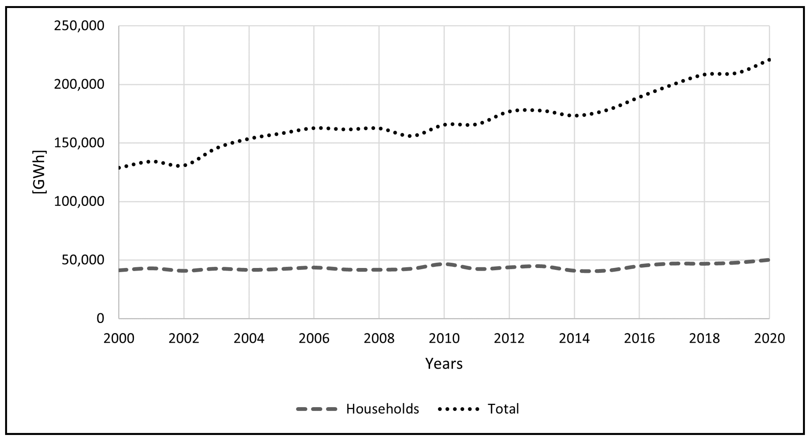
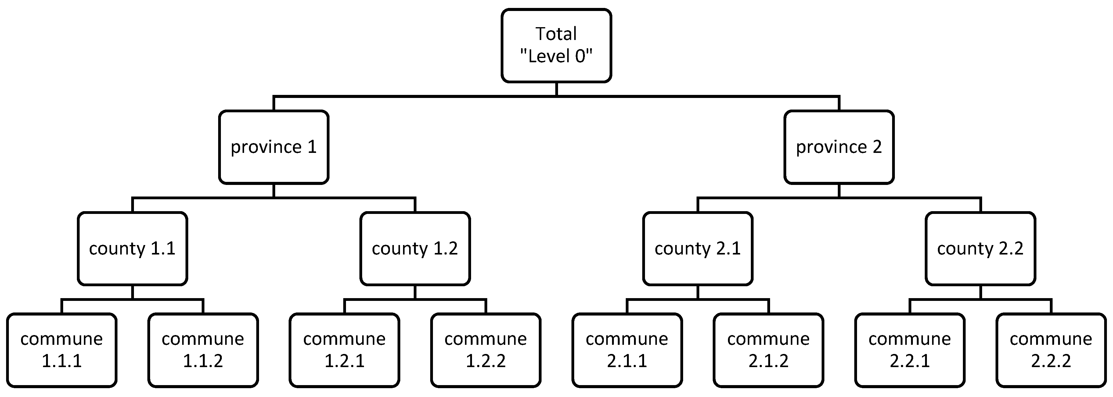
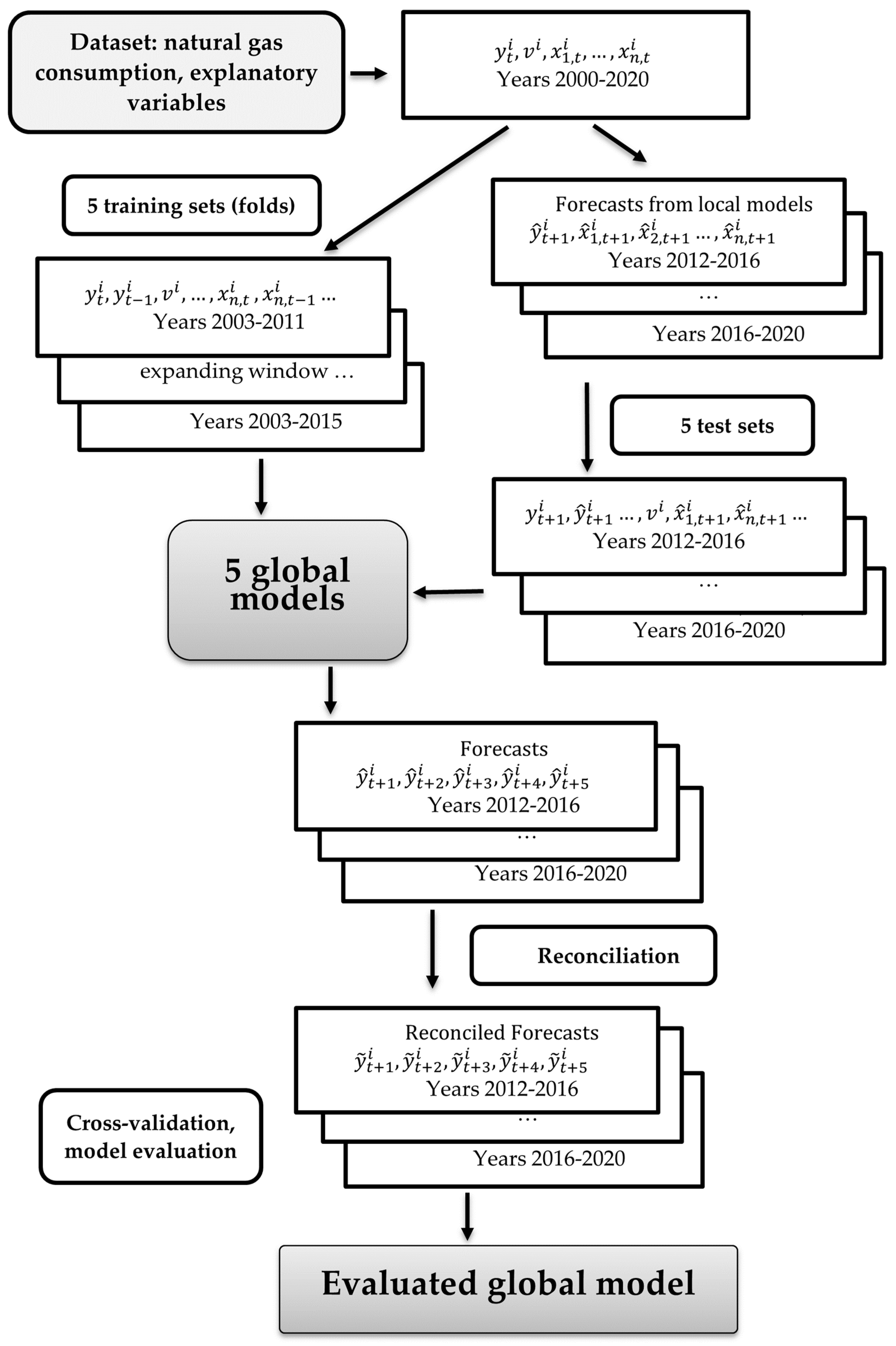
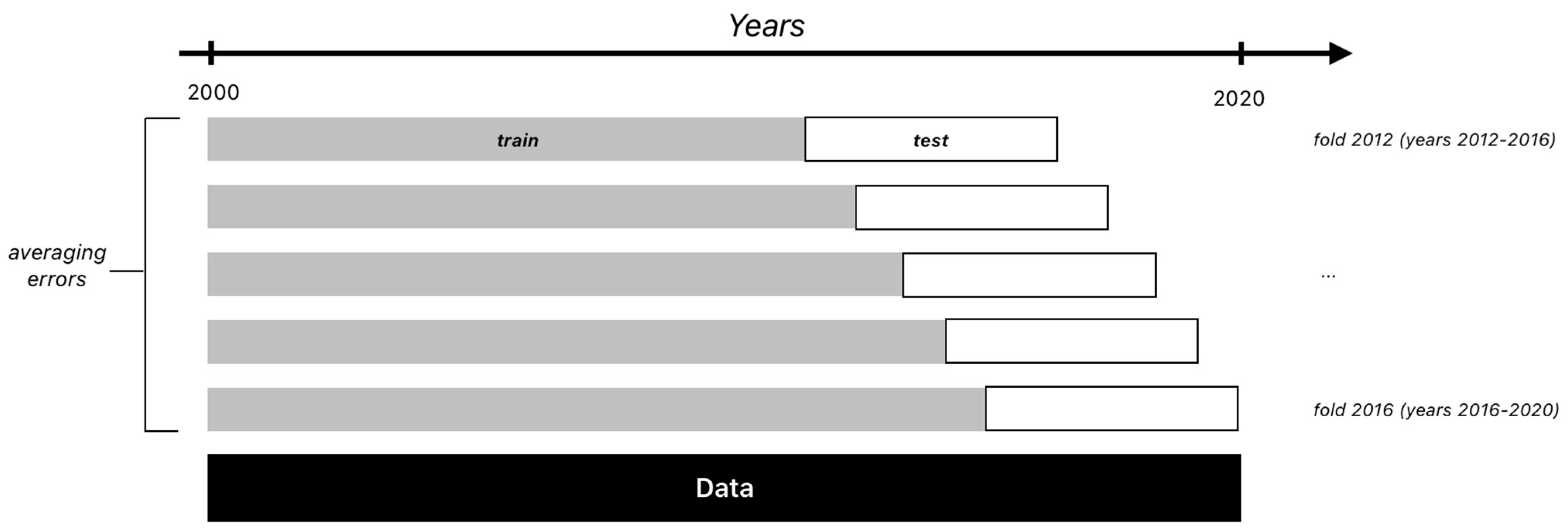
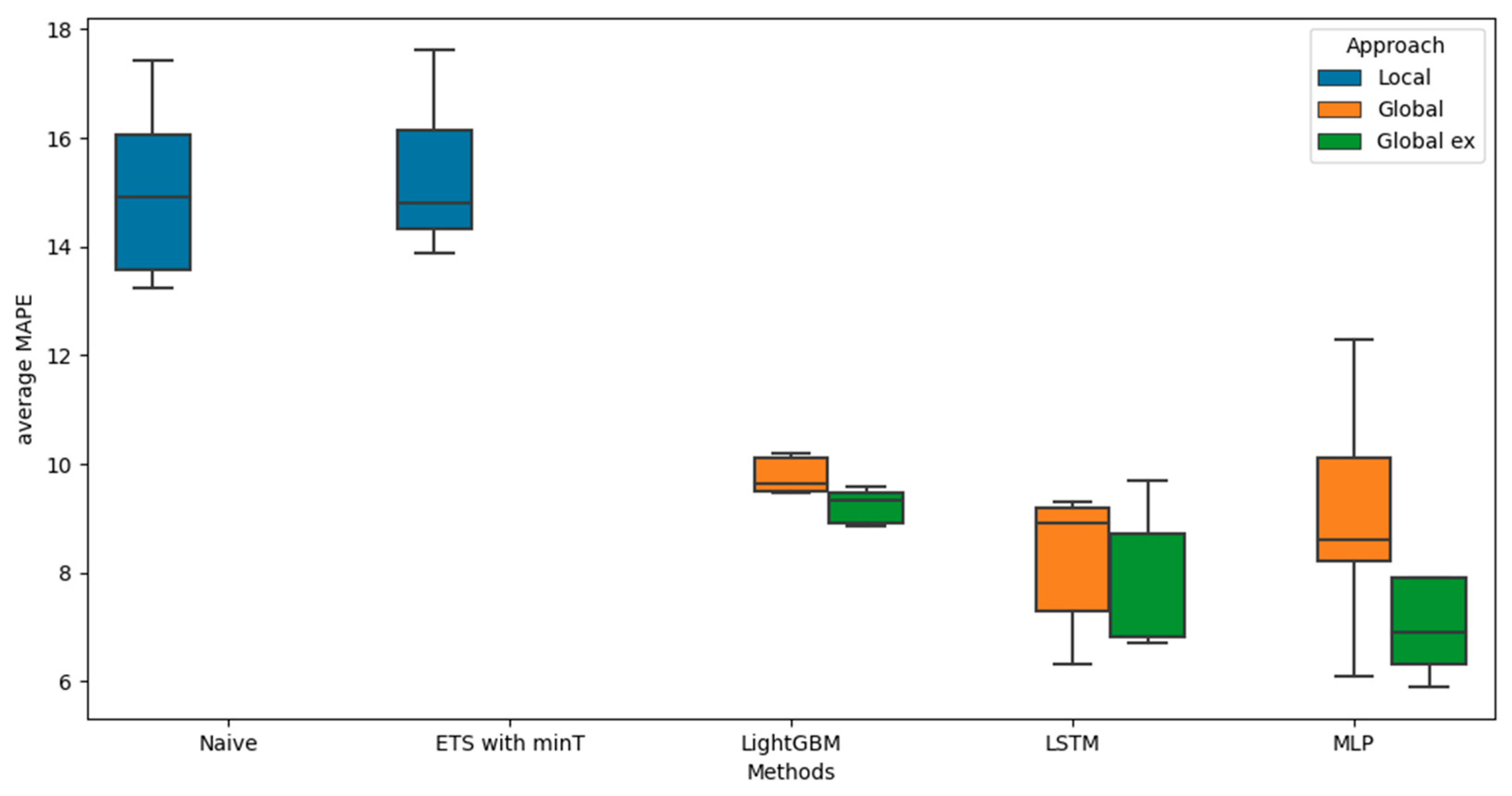
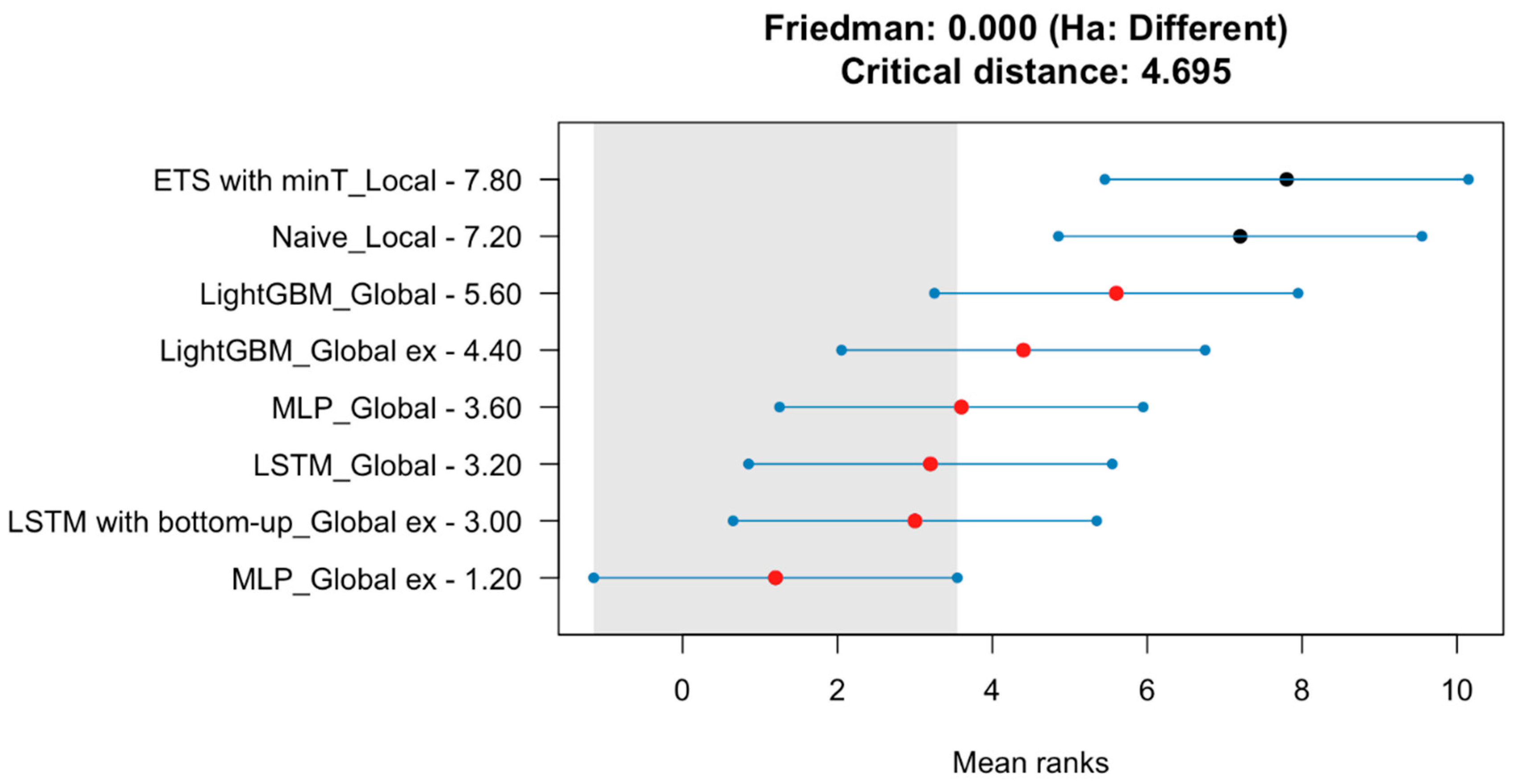
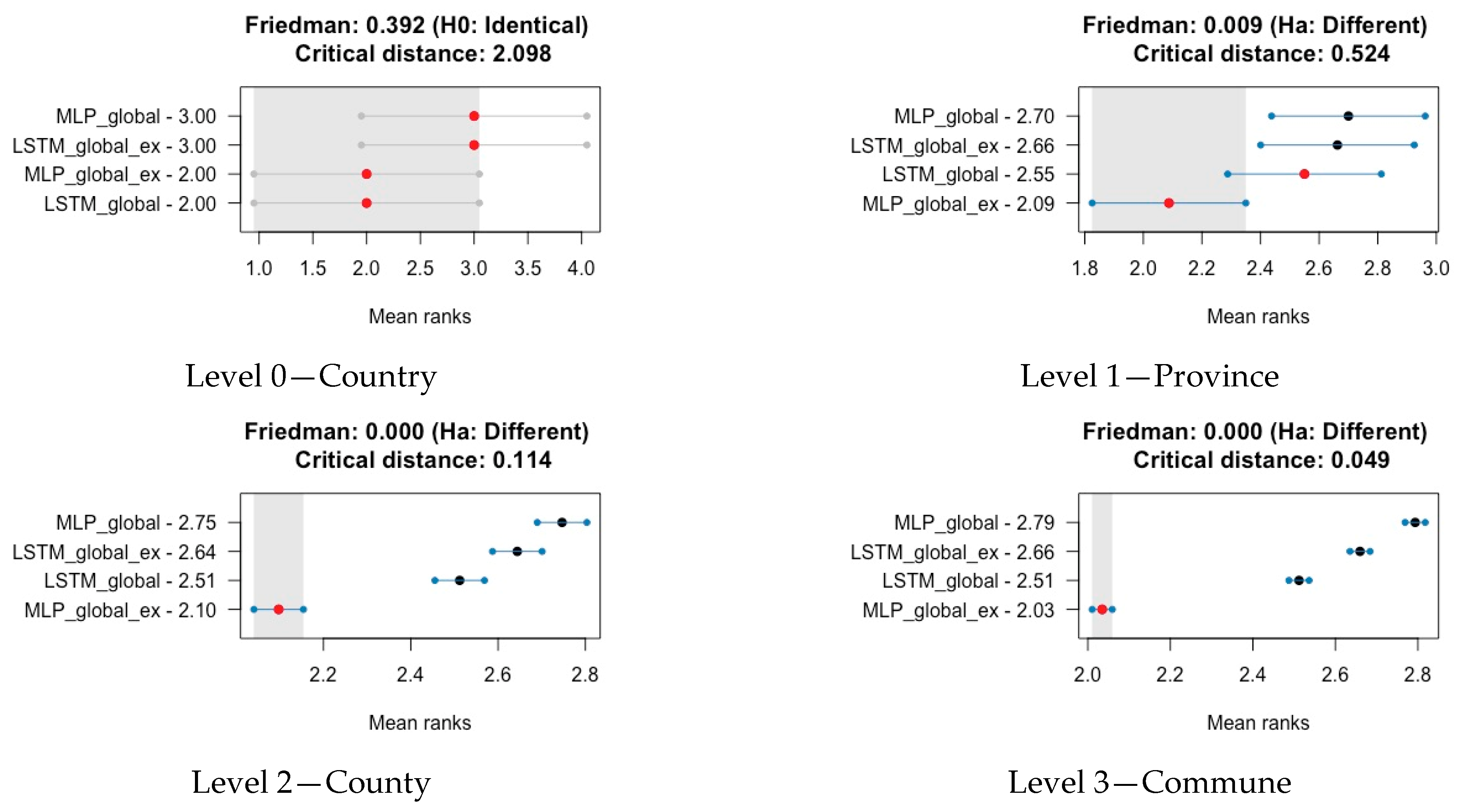
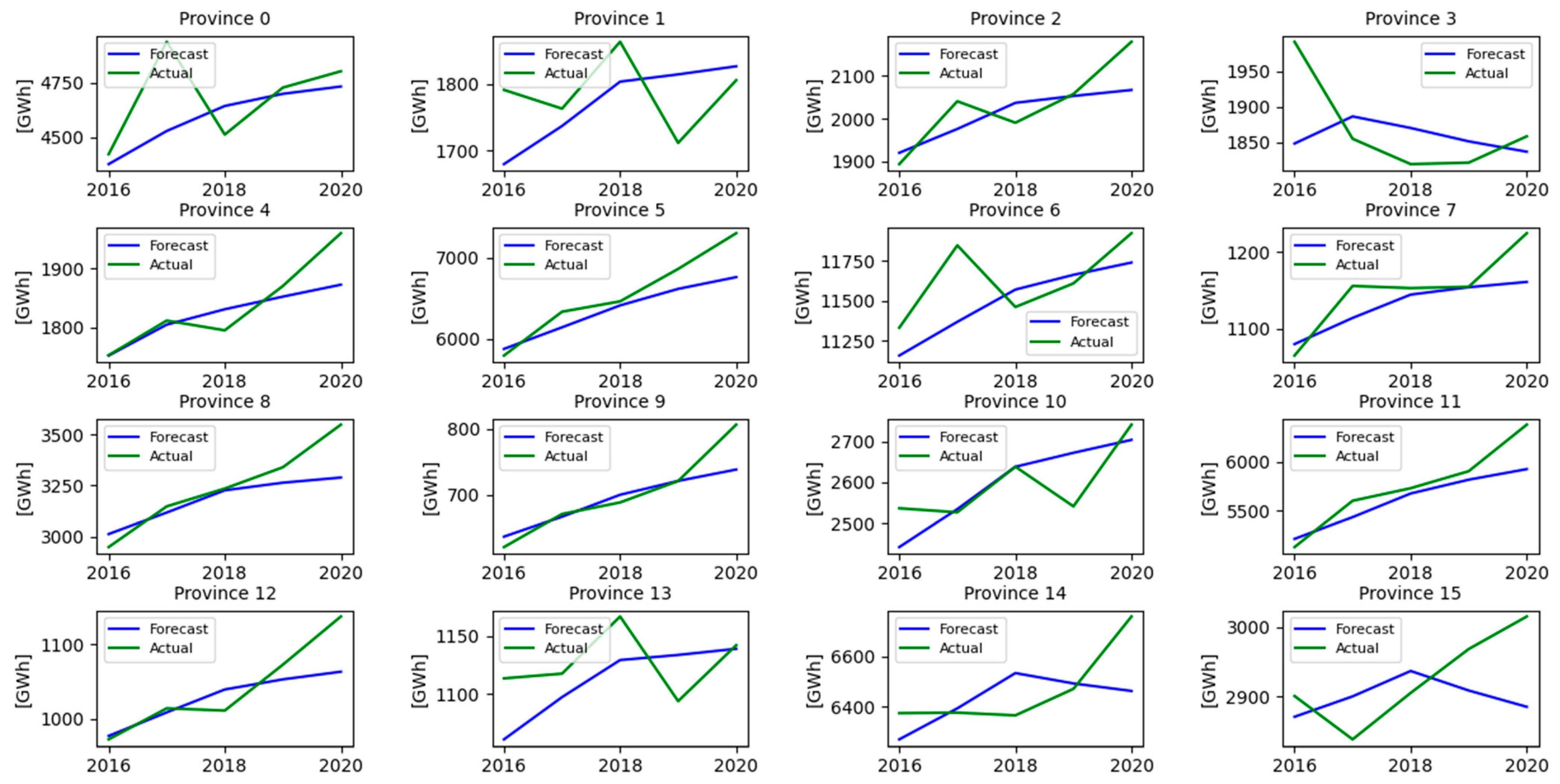
Table 1.
Hierarchy of the data set.
| Level | Number of Series | Total Observations per Level |
|---|---|---|
| Country | 1 | 21 |
| Province (voivodship) | 16 | 361 |
| County | 341 | 7149 |
| Municipality (commune) | 1851 | 38,791 |
Table 2.
Preselected variables for forecasting natural gas consumption.
| Variable | Explanation |
|---|---|
| population | Total number of inhabitants of a given territorial unit |
| households | Number of households in a given territorial unit |
| households with gas access | Number of households with access to the gas network |
| dwellings | Number of apartments or single-family homes in a territorial unit |
| dwellings built in a given year | Number of apartments or single-family homes commissioned in a given year in the area of a given unit |
| length of a gas network | Total length of the gas distribution network in a given territorial unit |
The value of the variable for the superior unit is the sum of the values of the subordinate units.
Table 3.
Descriptive statistics of explanatory variables.
| Variable | Level | ||||
|---|---|---|---|---|---|
| Country | Province | County | Municipality | ||
| Gas consumption [MWh] | avg | 52,095,287 | 3,255,956 | 152,773 | 28,145 |
| std | 3,152,298 | 2,626,010 | 261,999 | 103,042 | |
| max | 58,584,612 | 11,920,993 | 3,508,185 | 3,508,185 | |
| min | 47,861,391 | 477,309 | 16 | 3 | |
| population | avg | 35,470,005 | 2,216,876 | 104,018 | 19,163 |
| std | 176,351 | 1,310,045 | 129,364 | 58,184 | |
| max | 35,603,931 | 5,100,691 | 1,794,166 | 1,794,166 | |
| min | 35,158,436 | 594,578 | 4302 | 1021 | |
| households with gas access | avg | 8,408,569 | 525,536 | 24,659 | 4543 |
| std | 428,245 | 343,761 | 46,467 | 20,823 | |
| max | 9,522,706 | 1,608,416 | 687,908 | 687,908 | |
| min | 7,938,363 | 113,846 | 1 | 0 | |
| dwellings | avg | 13,061,565 | 816,348 | 38,304 | 7057 |
| std | 661,606 | 507,996 | 61,718 | 27,915 | |
| max | 14,200,526 | 2,300,920 | 1,020,433 | 1,020,433 | |
| min | 12,067,040 | 209,748 | 1694 | 243 | |
Table 4.
Parameters of neuron networks.
| Parameter | LSTM, MLP Local | LSTM, MLP Global |
|---|---|---|
| Input layer—number of neurons | 9 | 16 |
| Hidden layer—number of neurons | 6 | 8 |
| Dropout rate | 0.4 | 0.4 |
| Learning rate | 0.001 | 0.001 |
| Number of epochs | 20 | 20 |
Table 5.
Average performance of local models without reconciliation.
| MAPE [%] | RMSE | |
|---|---|---|
| Train | ||
| auto ARIMA | 12.2 | 7325 |
| auto EST | 10.7 | 7745 |
| NAÏVE (benchmark) | 13.2 | 8716 |
| 3-MA | 14.5 | 8748 |
| Test | ||
| auto ARIMA | 17.2 | 10,476 |
| auto EST | 15.6 | 9423 |
| NAÏVE (benchmark) | 15.0 | 10,068 |
| 3-MA | 15.2 | 9120 |
Table 6.
Average performance of ETS local models with different reconciliation methods.
| MAPE | RMSE | |
|---|---|---|
| Top-down | 15.6 | 9423 |
| Bottom-up | 15.6 | 9370 |
| Min-T | 15.4 | 9368 |
| Middle-out | 15.5 | 9348 |
Bold font indicates the best result.
Table 7.
Average performance of global models for hierarchical forecast reconciled with middle-out approach.
Table 7.
Average performance of global models for hierarchical forecast reconciled with middle-out approach.
| Method | Approach | MAPE [%] | RMSE |
|---|---|---|---|
| LightGBM Global | Global univariate | 9.8 | 7729 |
| LSTM Global | Global univariate | 8.5 | 5476 |
| MLP Global | Global univariate | 9.2 | 7264 |
| LightGBM Global ex | Global multivariate | 9.2 | 7189 |
| LSTM Global ex | Global multivariate | 7.8 | 5478 |
| MLP Global ex | Global multivariate | 7.1 | 4970 |
Bold font indicates the best result.
Table 8.
Detailed performance of global models for different levels of hierarchical forecast reconciled with middle-out approach averaged across all folds 2012–2016.
Table 8.
Detailed performance of global models for different levels of hierarchical forecast reconciled with middle-out approach averaged across all folds 2012–2016.
| Method | Approach | Level 0 Country | Level 1 Province | Level 2 County | Level 3 Commune |
|---|---|---|---|---|---|
| MAPE [%] | |||||
| LSTM | Global univariate | 3.5 | 4.3 | 6.5 | 8.8 |
| MLP | Global univariate | 5.1 | 5.6 | 7.3 | 9.6 |
| LSTM Global ex | Global multivariate | 3.7 | 4.3 | 6.1 | 8.1 |
| MLP Global ex | Global multivariate | 3.3 | 4.0 | 5.6 | 7.3 |
| RMSE | |||||
| LSTM | Global univariate | 2,104,511 | 156,496 | 10,266 | 2153 |
| MLP | Global univariate | 3,251,453 | 221,999 | 12,928 | 2611 |
| LSTM Global ex | Global multivariate | 2,321,036 | 168,800 | 10,116 | 2046 |
| MLP Global ex | Global multivariate | 1,971,673 | 147,538 | 9192 | 1897 |
Bold font indicates the best result.
Table 9.
Performance of global models for hierarchical forecast reconciled with middle-out approach in consecutive folds.
Table 9.
Performance of global models for hierarchical forecast reconciled with middle-out approach in consecutive folds.
| Method | Fold | 2012 | 2013 | 2014 | 2015 | 2016 |
|---|---|---|---|---|---|---|
| MAPE [%] | Approach | |||||
| LSTM | Global univariate | 9.1 | 9.4 | 9.8 | 7.6 | 6.4 |
| MLP | Global univariate | 8.3 | 8.7 | 10.8 | 12.0 | 6.1 |
| LSTM Global ex | Global multivariate | 9.7 | 8.7 | 6.7 | 6.8 | 6.8 |
| MLP Global ex | Global multivariate | 7.9 | 7.9 | 6.9 | 6.3 | 5.9 |
| RMSE | ||||||
| LSTM | Global univariate | 5321 | 6163 | 6939 | 5088 | 3866 |
| MLP | Global univariate | 5767 | 6898 | 7922 | 11,874 | 3857 |
| LSTM Global ex | Global multivariate | 6392 | 6468 | 4419 | 5359 | 5112 |
| MLP Global ex | Global multivariate | 5775 | 5740 | 5260 | 4651 | 3537 |
Table 10.
Comparison of computational time.
| Method | Approach | Computational Time [h] |
|---|---|---|
| Benchmark | Local | 0.02 |
| ETS with reconciliation | Local | 0.04 |
| LightGBM | Global univariate | 0.06 |
| LSTM Global | Global univariate | 0.30 |
| MLP Global | Global univariate | 0.25 |
| LSTM Global ex | Global multivariate | 0.80 |
| MLP Global ex | Global multivariate | 0.40 |
Disclaimer/Publisher’s Note: The statements, opinions and data contained in all publications are solely those of the individual author(s) and contributor(s) and not of MDPI and/or the editor(s). MDPI and/or the editor(s) disclaim responsibility for any injury to people or property resulting from any ideas, methods, instructions or products referred to in the content. |
© 2024 by the authors. Licensee MDPI, Basel, Switzerland. This article is an open access article distributed under the terms and conditions of the Creative Commons Attribution (CC BY) license (https://creativecommons.org/licenses/by/4.0/).
Share and Cite
MDPI and ACS Style
Gaweł, B.; Paliński, A. Global and Local Approaches for Forecasting of Long-Term Natural Gas Consumption in Poland Based on Hierarchical Short Time Series. Energies 2024, 17, 347. https://doi.org/10.3390/en17020347
AMA Style
Gaweł B, Paliński A. Global and Local Approaches for Forecasting of Long-Term Natural Gas Consumption in Poland Based on Hierarchical Short Time Series. Energies. 2024; 17(2):347. https://doi.org/10.3390/en17020347
Chicago/Turabian StyleGaweł, Bartłomiej, and Andrzej Paliński. 2024. "Global and Local Approaches for Forecasting of Long-Term Natural Gas Consumption in Poland Based on Hierarchical Short Time Series" Energies 17, no. 2: 347. https://doi.org/10.3390/en17020347
Note that from the first issue of 2016, this journal uses article numbers instead of page numbers. See further details here.