Communicationless Overcurrent Relays Coordination for Active Distribution Network Considering Fault Repairing Periods

Abstract

This paper presents an integrated overcurrent relays coordination approach for an Egyptian electric power distribution system. The protection scheme suits all network topologies, including adding distribution generation units (DGs) and creating new paths during fault repair periods. The optimal types, sizes, and locations of DGs are obtained using HOMER software (Homer Pro 3.10.3) and a genetic algorithm (GA). The obtained values align with minimizing energy costs and environmental pollution. The proposed approach maintains dependability and security under all configurations using a single optimum setting for each relay. The calculations consider probable operating conditions, including DGs and fault repair periods. The enhanced coordination procedure partitions the ring into four parts and divides the process into four paths. The worst condition of two cascaded overcurrent relays from the DGs’ presence viewpoint is generalized for future work. Moreover, a novel concept addresses the issue of insensitivity during fault repair periods. The performance is validated through the simulation of an Egyptian primary distribution network.

1. Introduction

The possession of advanced and stable electric power systems has become an urgent necessity for each country to keep pace with the industrial and technological development that is gripping the world in all walks of life [1]. Electrical energy demands are growing continuously, requiring an increase in generation capacity. This leads to a growing increase in generation costs, environmental pollution, and global warming. Therefore, system designers must search for alternative clean and economical sources. Also, the higher cost of transmission and distribution losses motivates system planners to use these alternatives as distributed generation units (DGs) in electrical distribution networks. The complication of protective device coordination in interconnected power subtransmission systems and deregulated distribution systems is intensively increasing due to continuous changes in the interconnected systems’ topology [2]. These changes result from sustained load growth and the corresponding installation of distributed generation units (DGs). In recent times, various distributed generation units (DGs) have been integrated into interconnected power systems due to their advantages over installing remote generation stations [3,4]. To fully leverage the presence of DGs in the system, extensive studies have been conducted in the literature [5].

As per the survey conducted by Electric Power Research and Natural Gas Institutions, the electric power generation shared by distributed generation units (DGs) is estimated to reach approximately 30% of the total power [6,7]. The types of DGs include small gas turbines, microturbines, fuel cells, wind, and solar energy. The literature has addressed the optimal allocation of DGs considering fuel cost savings and demand variation, as demonstrated in [8]. However, the integration of DGs has some adverse effects on the reliability and speed of the protection system [9]. The protection system may become unreliable due to incorrect operation or insensitivity (blinding) issues with protective devices. Slower protection system response (increased protection time) could result in exceeding the thermal capacity limit of electrical equipment, such as a transformer during close-in faults. These negative effects are influenced not only by changes in the level and direction of the fault current but also by the potential mismatch in fault current levels between coordinated relay pairs. On the other hand, another challenge for overcurrent relays coordination is ensuring the continuity of the distribution system by connecting the bus coupler (BC). If there is a fault in the feeder, the corresponding overcurrent relays would issue a tripping signal to isolate the fault. This leads to disconnecting healthy loads, especially when the fault is close to the upstream section. Connecting the BC ensures the supply of power to these loads from another direction. However, the direction and magnitude of current change in some sections, leading to relays miscoordination.

In [10], a coordination method utilizing directional overcurrent relays with nonstandard characteristics is presented to cancel the negative effect of the DGs’ presence while enhancing the protection speed. In [11], a coordination technique based on a new coordination index determined by a two-phase nonlinear programming method is presented to reduce both the number of adaptive relays and the total operating time of the installed relays. In [12], an optimum coordination method considering the high penetration of DGs is presented, which reduces the total operating time by utilizing the adaptive modified firefly optimization algorithm.

Another trend to mitigate the effect of DGs on the reliability and speed of the protection system is by adding fault current limiters (FCLs), either in series with DGs or at different locations within the distribution sections [13,14]. In [15], the minimization of the FCLs values, with the permission to readjust the original setting of only one overcurrent relay, is accomplished. However, the techniques presented in [13,14,15] increase the cost due to the addition of FCLs.

In [16,17,18,19], the proper settings are selected, and the proper coordination is maintained by exchanging data between the agents installed at different points in electric distribution systems, such as DGs and relay locations, through the installed communication channels. In [16], an adaptive overcurrent relays coordination system activating the best settings for each operating condition is presented with the aid of the centralized control method (SCADA system) that monitors the system configuration and DGs status. Consequently, the centralized agent determines the corresponding optimum settings utilizing the differential evolution algorithm and then updates the relays’ settings via the communication channels. In [17], the communication simulation of agents is enhanced, and the case of primary protection failure is covered by operating the nearest backup function. In [18], the adaptive overcurrent relays coordination covers the existence of both parallel feeders and DGs presence by exchanging the data on both the operating condition of the two parallel feeders and the current direction of these feeders. In [19], the negative effect of DGs’ presence on overcurrent relay–recloser–fuse protection of distribution systems is cancelled by transferring the measured currents at fuse locations to select the adequate setting of the fast curve of the recloser.

Recently, there has been a growing interest in implementing intelligent methods in protection systems by utilizing communication infrastructure and intelligent electronic devices (IEDs). Notably, various intelligent techniques have been highlighted in [20,21,22,23,24], employing multi-agent systems (MASs). These MASs enable the exchange of distribution network data among agents, thereby enhancing the protection system’s performance. For instance, in [20], an intelligent protection scheme is presented, which utilizes a centralized and multilayered MAS to interact with relays, DGs, and loads, ensuring effective protection coordination. Another approach, detailed in [21], introduces a MAS-based self-healing protection scheme that adapts to varying network conditions. Furthermore, Ref. [22] introduces a self-healing protection system utilizing a MAS comprising feeder, zone, breaker, and DG agents. Additionally, Ref. [23] proposes a protection system that combines MAS and machine learning algorithms to coordinate and update the protection scheme, allowing adaptation to new network conditions. In [24], the proper delaying time is activated through communication between the neighboring relays. It is essential to consider that the performance of MAS-based protection systems is significantly influenced by the implementation of communication links between agents, as well as the number and type of agents involved. Additionally, the reliability of the protection system depends on the communication system’s reliability, which can be affected by both cyberattacks and the risk of communication failures. Consequently, the complexity of coordinating the relays without the need for communications, while considering both the busbar coupler operation and the self-healing process (during fault repairing periods), represents a challenge for protection engineers, particularly in the presence of multiple DGs.

The main contribution of this paper is presenting a novel coordination approach to maintain both dependability and security attributes for active distribution systems. This approach considers fault repair periods and the presence of multiple DGs, while utilizing a single optimum setting for each relay. The coordination procedure is based on partitioning the ring into four parts and dividing the process into four paths (four subroutine algorithms). The worst condition of each two cascaded overcurrent relays from the viewpoint of DGs is generalized for future work. Additionally, a new idea overcomes the insensitivity problem during fault repair. The performance of the proposed approach is examined through the simulation of an actual Egyptian primary distribution network.

The content of the following sections is outlined as follows: the illustration of the test system is in Section 2. The optimal allocation of distributed generation units is presented in Section 3, which includes both the HOMER-based model for selecting suitable DGs and DG sizing in Section 3.1, and the GA-based model for DG siting in Section 3.2. Conventional overcurrent relays coordination is discussed in Section 4, covering the procedure of conventional coordination in Section 4.1 and the effect of DGs’ presence on conventional coordination in Section 4.2. Section 5 introduces the modified overcurrent relays coordination for distribution systems with distributed generation units, including coordination of forward relays, coordination of backward relays, and the evaluation of the modified coordination under opening bus coupler in Section 5.1, Section 5.2 and Section 5.3, respectively. To consider fault repairing periods, including the case of closing bus coupler, a new communicationless overcurrent relays coordination approach for deregulated distribution systems is introduced in Section 6. Section 6.1 illustrates the concept of the proposed communicationless Overcurrent Relays Coordination, while Section 6.2 illustrates the procedure for the computation of the new coordination approach. Section 7 contains the evaluation of the new protection coordination approach. Finally, the conclusion is presented in Section 8.

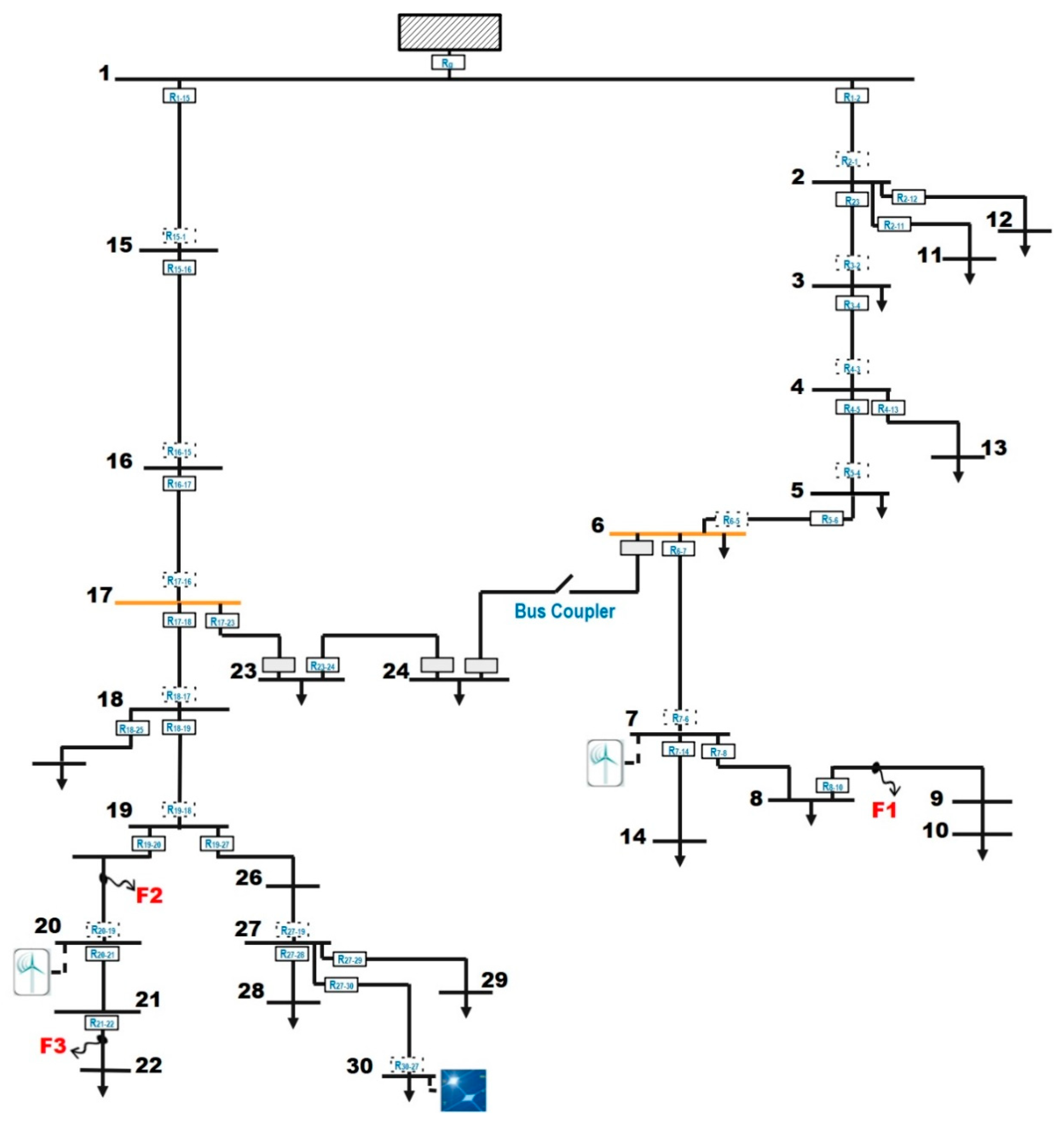
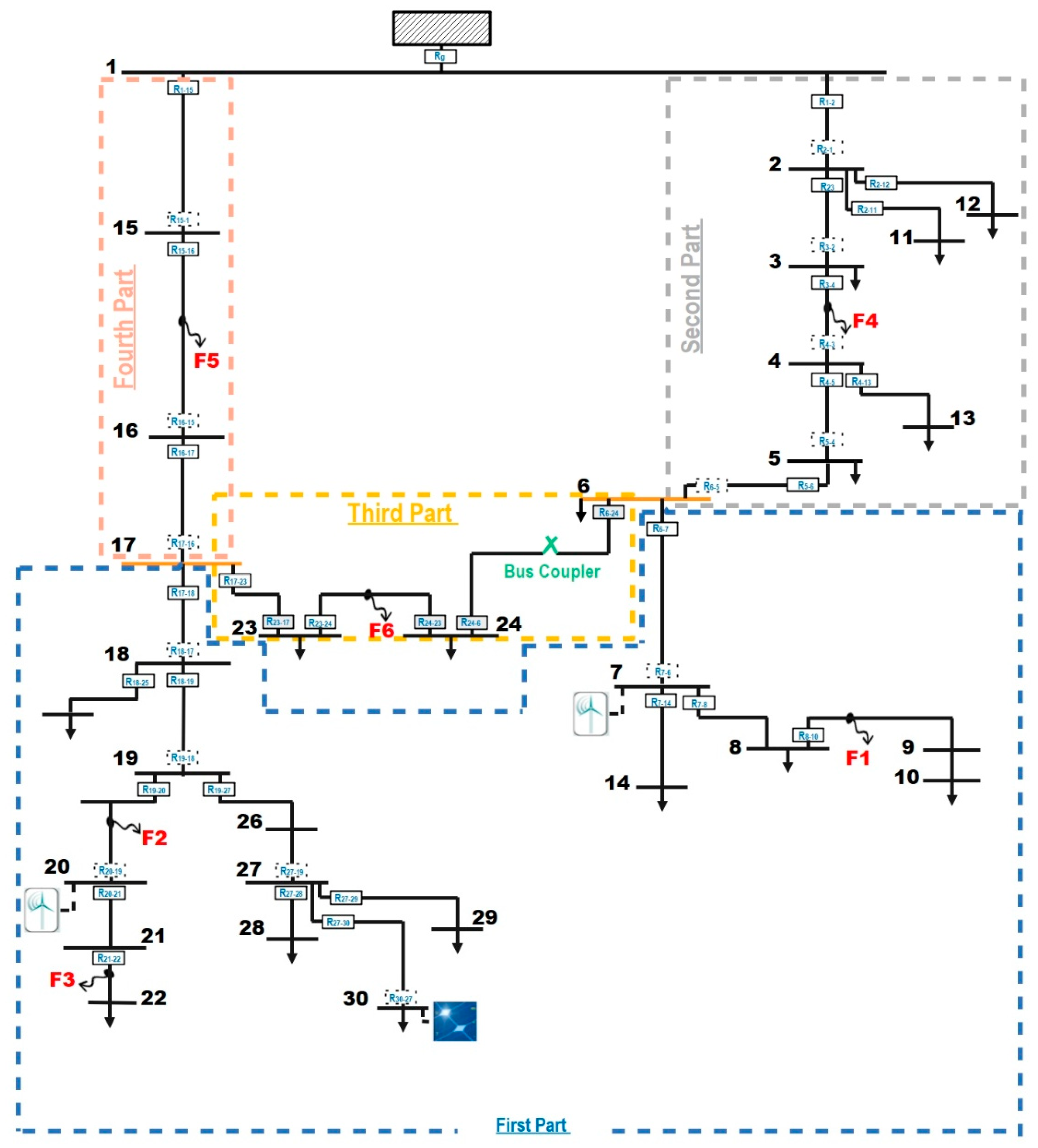
2. Test System

In this paper, an 11 kV primary distribution network located in Sadat City is used as an actual test system, as shown in Figure 1. The network has 30 busbars, divided into two feeders with a total load of 10.054 MW and 7.8 MVAR. The system data are given in Appendix A. Load flow calculations are carried out, and their results indicate the presence of four overloaded sections (1–2, 1–15, 15–16, and 16–17) with power losses of 133.9 kW. To relieve the overloaded lines and minimize the power losses in the considered system, an optimal allocation study for adding distributed generation units is accomplished in the next section.

3. Optimal Allocation of Distributed Generation Units

The incorporation of distributed generation units (DGs) into distribution networks involves two main issues. The first issue is determining the type and penetration level of each DG, considering economic and emission performance within the system. This aspect is addressed using HOMER software, which focuses on the generation units and load of the network, regardless of the network configuration. HOMER software optimally selects suitable DGs and determines their penetration level. The second issue involves determining the optimal location for each DG unit within the distribution network. This problem is treated using a genetic algorithm, which serves as an optimization tool to find the optimal locations of the DG units while considering various network constraints. These issues are summarized in the flowchart illustrated in Figure 2.

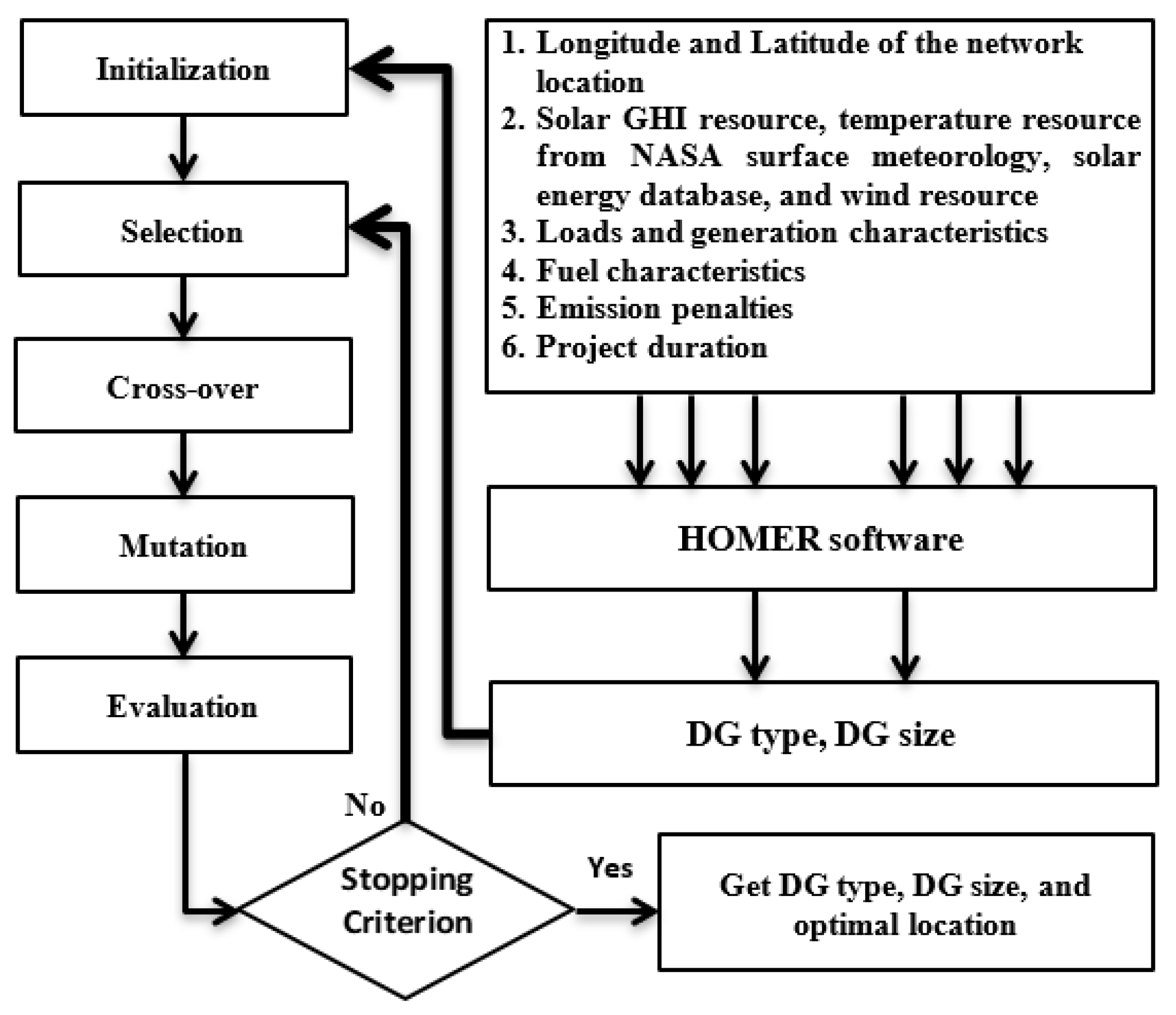
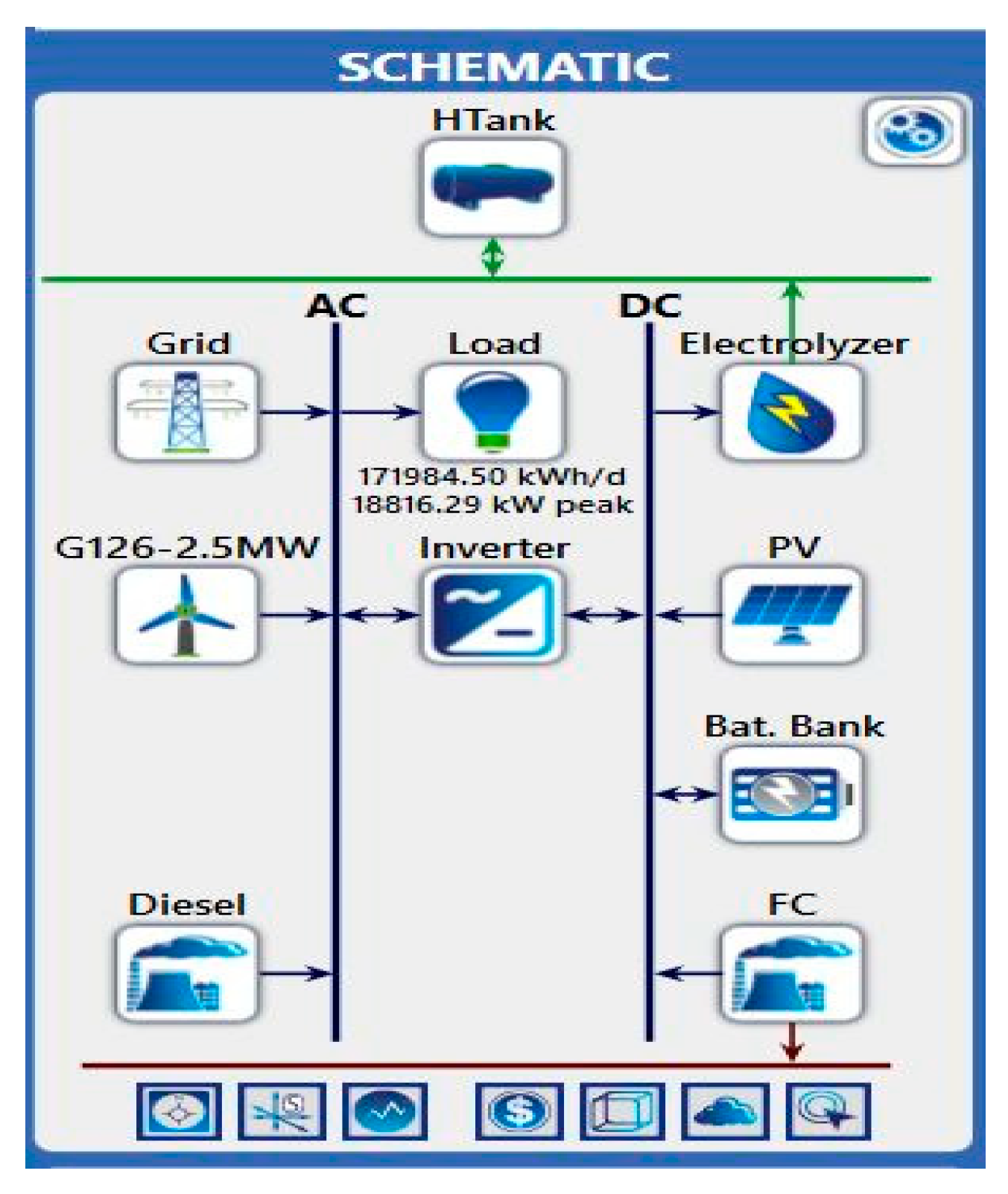
3.1. HOMER-Based Model for Selecting Suitable DGs and DG Sizing

The objective is to minimize the total energy cost (COE) supplied to the loads by DGs in conjunction with the grid, utilizing HOMER software. The overall cost is expressed as follows [25]:

$$C_{\mathit{total}}=C_{\mathit{grid}}+C_{\mathit{PV}}+C_{\mathit{WT}}+C_D+C_{\mathit{FC}}+C_{\mathit{Batt}.}+C_{\mathit{inv}}-C_{\mathit{sold} E}$$

(1)

where:

• $C_{\mathit{grid}}$ is the cost of energy used from the grid ($).
• $C_{\mathit{PV}}$ is the photovoltaic arrangement cost ($).
• $C_{\mathit{WT}}$ is the wind turbine cost ($).
• $C_D$ is the diesel generator cost ($).
• $C_{\mathit{FC}}$ is the fuel cell cost ($).
• $C_{\mathit{Batt}.}$ is the battery bank cost ($).
• $C_{\mathit{inv}}$ is the cost of the inverter ($).
• $C_{\mathit{sold} E}$ is the cost of energy delivered to the grid ($).

The cost function of the ith DG is formulated as [26]:

$$C_i=N_i · \left[C_{cap,i}+O\&M_i+K_i · C_{rep,i}-S_i\right]$$

(2)

where:

• $N_i$ is the number of inserted DG.
• $C_{\mathit{cap},i}$ is the capital cost of DG ($).
• $O\&M_i$ is the operation and maintenance cost of DG ($).
• $K_i$ is the number of replacements for DG.
• $C_{\mathit{rep},i}$ is the replacement cost of DG ($).
• $S_i$ is the salvage amount of DG ($).

The constraints are listed in the following equations.

$$P_{DG\left(i\right)}{}^{\mathit{min}}\le P_{\mathit{DG}\left(i\right)}\le P_{\mathit{DG}\left(i\right)}{}^{\mathit{max}}$$

(3)

$${\displaystyle \sum }_{i=1}^N{P}_{\mathit{DG}\left(i\right)}+P_{\mathit{grid}}=P_{\mathit{LD}}$$

(4)

where:

• $P_{\mathit{DG}\left(i\right)}$ is the output power of DG (kW).
• $P_{\mathit{grid}}$ is the grid power (kW).
• $P_{\mathit{LD}}$ is the load demand (kW).

HOMER considers the network in two parts: generators and loads, while ignoring losses. Various types of DGs could be installed, such as photovoltaic (PV), wind turbine (WT), fuel cell (FC), batteries (B), and diesel generators (D). Each DG has its own characteristics that must be defined. Additionally, the load curve must be carefully defined for accurate DG sizing. Four steps are required to model a system in HOMER:

• Obtaining the longitude and latitude of the network location.
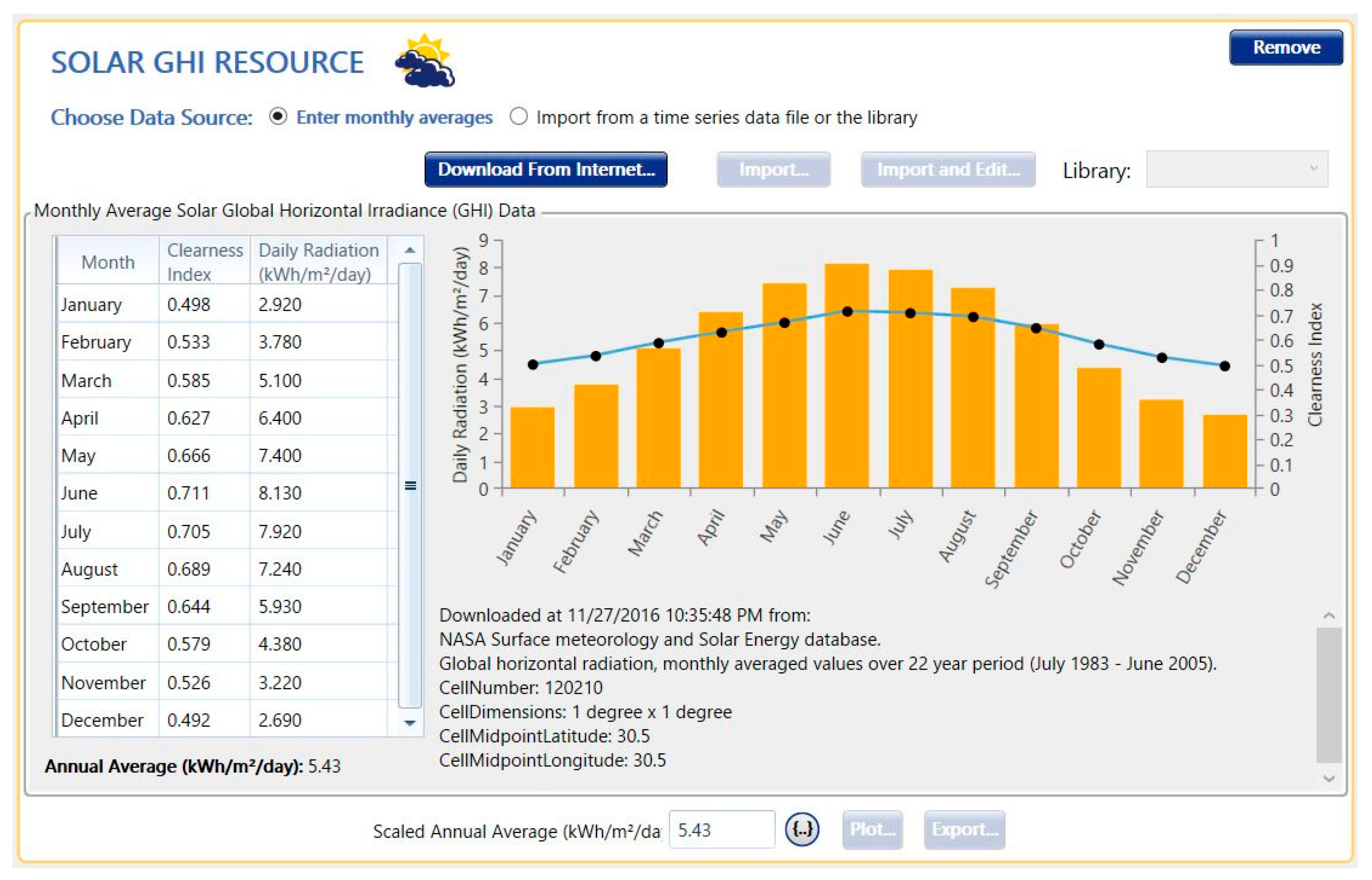
• Downloading the Solar Global Horizontal Irradiance (GHI) resource, temperature resource from NASA surface meteorology, solar energy database, and wind resource [27].
• Adding the characteristics of both loads and generation.
• Defining the fuel characteristics, the emission penalties, and finally the project duration.

By implementing these steps in the Egyptian distribution network, five DG units (WT, PV, Diesel, FC, and battery bank) can be simulated utilizing HOMER. The grid and DG standards are as follows:

• The grid power price and grid sellback price are 0.087 $/kWh.
• The solar system is composed of stationary flat-plate PV with a lifetime of 25 years and an 80% derating factor. The maximum available space for PV is 1000 kW, obtained by utilizing the ready area to install a PV substation at the studied network location, where each kW requires a minimum area of 10 m². The Solar Global Horizontal Irradiance (GHI) resource is depicted in Figure 3.
• The Gamesa G126-2.5MW wind turbine with a lifetime of 20 years is utilized. Its hub height is 102 m, and the power curve of the wind turbine is illustrated in Figure 4. The average wind speed per year is 4.85 m/s [28].
• A diesel generator with a maximum available space of 1000 kW is utilized; however, the price of diesel fuel is 299 × 10⁻³ $/L.
• A general fuel cell with a maximum available area of 100 kW is utilized, where hydrogen is used as fuel. The electrolyzer and hydrogen tank are utilized to supply the fuel cell with the hydrogen needed to operate.
• A battery bank, modified kinetic battery model, with a voltage of 2 V and a capacity of 1 kWh using a maximum available area of 30 batteries is utilized.
• Carbon dioxide needs to be removed from the atmosphere [29].

On the other hand, the load standards of the studied Egyptian distribution network consist of 10.054 MW, with the load profile illustrated in Figure 5. Figure 6 depicts the system in the HOMER software. The costs of the system components, including initial, replacement, operation, and maintenance, are listed in

Table 1. The costs of the system components.

Component (Capacity/Quantity)	Capital Cost ($)	Replacement Cost ($)	Operation & Maintenance Cost ($)
PV (1 kW)	0.9 × 103	0.9 × 103	0
WT (2.5 MW)	5.5 × 106	5.5 × 106	9 × 104/year
Diesel (1 kW)	0.5 × 103	0.5 × 103	0.03/h
FC (1 kW)	3 × 103	2.5 × 103	0.01/h
Battery (2 V)	0.3 × 103	0.3 × 103	10/year
Electrolyzer (0.15 kW)	0.6 × 103	0.6 × 103	2/year
Hydrogen Tank (1 kg)	0.02 × 103	0.02 × 103	0.05/year

. The study is conducted for 20 years, which is the average lifetime of the considered components. The optimum types and sizes of DGs are obtained using HOMER, as listed in

Table 2. HOMER optimization results.

Items		Optimum Results
Architecture	PV (kW)	1000
	WT (G126—2.5 MW)	2
	Inverter (kW)	680
Cost	COE ($/kWh)	0.0861
	NPC ($)	63 M
	Operating cost ($)	4.39 M
	Initial capital ($)	12.1 M
System	Renewable fraction (%)	33.6
PV	Capital cost ($)	900,000
	Production (kWh)	1,540,204
WT (G126—2.5 MW)	Capital cost ($)	11,000,000
	Production (kWh)	19,717,122
	O&M cost ($)	180,000
Grid	Energy purchased (kWh)	41,921,056
	Energy sold (kWh)	361,485

.

3.2. GA-Based Model for DG Siting

The output of the HOMER-based model is the optimal types and sizes of the DG units that improve the economic and emission performance of the Egyptian distribution network. The selected types of DG units should be optimally sited across the distribution network, considering the configuration and operation constraints. GA is applied as a well-established optimization technique to handle the siting problem of the DG units in the distribution network. The main objective of the optimization problem is to minimize the total power loss while maintaining voltage regulation within a safe range in the primary distribution network. This optimization problem can be formulated as follows:

The objective function,

$$\mathit{Minimize} P_{\mathit{loss}}={\displaystyle \sum }_{k=1}^{\mathit{nl}}{\mathit{Ploss}}_k$$

(5)

The objective function is subjected to the following constraints:

$$P_{\mathit{grid}}+{\displaystyle \sum }_{i=1}^N{P}_{\mathit{DG}}=P_{\mathit{LD}}+P_{\mathit{loss}}$$

(6)

$$V_i{}^{\mathit{min}}\le V_i\le V_i{}^{\mathit{max}}$$

(7)

where the power losses in the network are computed based on the Forward–Backward Sweep algorithm using the following equation:

$${\mathit{Ploss}}_k=R_k \left[\begin{array}{c}{\left({\displaystyle {\displaystyle \sum }_{j=2}^{nb}}BIBC\left(k,j-1\right) · \frac{P_j cos{\theta }_j+Q_j sin{\theta }_j}{\left|V_j\right|}\right)}^2+\\ {\left({\displaystyle {\displaystyle \sum }_{j=2}^{nb}}BIBC\left(k,j-1\right) · \frac{P_j sin{\theta }_j-Q_j cos{\theta }_j}{\left|V_j\right|}\right)}^2\end{array}\right]$$

(8)

where:

• ${\mathit{Ploss}}_k$ is the active power loss of branch k.
• BIBC is the Bus-Injection to Branch-Current matrix.
• nl is the number of distribution system branches.
• nb is the number of the distribution system buses.
• $V$_j is the voltage magnitude at bus j.
• $\theta$_j is the voltage angle at bus j.
• $P$_j is the net consumed active power at bus j.
• $Q$_j is the net consumed reactive power at bus j.

GA is initialized with a population of random guesses that will be spread throughout the search space by applying three operators: selection, crossover, and mutation to generate new populations until reaching the optimal solution. GA is commonly utilized to solve various optimization problems in power systems. The total power loss in the network is treated as the objective function that needs to be minimized during the optimization process. Both the objective function and network constraints are calculated using the Forward–Backward Sweep algorithm.

The control variables of the optimal siting problem are the location and the output power generation of the DG units. The location control variable represents the busbar number, ranging from 2 up to the maximum number of buses in the distribution network. However, the DG output power control variable ranges from the minimum to the maximum power generation of each DG unit.

The results obtained from the GA-based DG siting algorithm show that siting the first WT at busbar 7, siting the second WT at busbar 20, and siting the PV station at busbar 30 are the optimal locations for the DG units. The total power loss decreased from 133.9 kW to 61.1 kW. The overloaded sections were relieved due to the optimal siting of the selected DGs.

4. Conventional Overcurrent Relays Coordination

The default configuration of the selected distribution system is that the bus coupler is disconnected, and no DGs are connected to the system. Therefore, an overcurrent relay upstream of each section is sufficient. Each relay is defined by two numbers. The first number represents the sending busbar, and the second one represents the receiving busbar. For example, for feeder (1-2), R_1-2 is the forward relay, as illustrated in Figure 1. To assess the effect of DGs penetration on conventional coordination, the procedure for conventional coordination should be performed as described in the following subsection.

4.1. The Procedure of the Conventional Coordination

The procedure for the conventional coordination between two cascaded inverse relays is detailed and illustrated in [18] by the same author. The Genetic Algorithm (GA) is utilized to verify the optimal coordination margins by minimizing the objective function, which is the sum of the operating times of the relays at the corresponding worst conditions. The objective function is verified under security constraints that ensure proper coordination between each pair of cascaded relays. The coordination constraints are incorporated into the objective function through an augmented fitness function, as shown in [18] by the same author. Initially, the coordination of the right-hand-side (RHS) relays from R_8-10 to R_1-2 in the considered system, as shown in Figure 1, is as follows: The downstream relays (R_2-11, R_2-12, R_4-13, R_7-14, R_8-10) are set to their lowest time dial setting (0.02 in numerical relays). The coordination constraint between relays R_7-8 and R_8-10 (downstream relays) is formulated as an inequality constraint (Z_CTI) using the maximum jointed fault current, as follows:

$$Z_{CTI}{}_1=\mathit{max}\{0 , (\mathit{min}CTI-(t_{\mathrm{R}7-8}-t_{\mathrm{R}8-10}))\}$$

(9)

Then, each pair of relays (11 pairs of relays) will be coordinated according to the maximum jointed fault current in the overlapped region, primarily protected by the inverse characteristic, for each pair of cascaded relays as shown in

Table 3. Maximum jointed fault current for each two cascaded pairs of relays of the RHS feeder.

No. of Pairs	Pair of Relays		IFmax (For Phase Faults) (A)	IFmax (For Earth Faults) (A)
	Backup	Primary
1	R7-8	R8-10	4596.4	4133.6
2	R6-7	R7-8	4696.3	4266.2
3	R6-7	R7-14	4711.4	4286.2
4	R5-6	R6-7	4769.1	4365.6
5	R4-5	R5-6	4874.4	4512.9
6	R3-4	R4-5	4941.6	4608.8
7	R3-4	R4-13	4943.7	4612.3
8	R2-3	R3-4	4969.5	4649.3
9	R1-2	R2-3	5028.3	4736
10	R1-2	R2-11	5037.5	4750
11	R1-2	R2-12	5038.4	4751.3

.

Finally, the fitness function for evaluating an individual in the population of the GA, containing the coordination margin among all relays in the RHS feeder, is:

$$\mathit{fitness}={{\displaystyle \sum }}_{i=1}^N{t}_i+{{\displaystyle \sum }}_{j=1}^{11}{K}_j·Z_{CTI}{}_j$$

(10)

where ‘i’ refers to the relay number, and ‘j’ refers to the number of pairs, which ranges from 1 to 11 as indicated in Table 3. K₁ is selected to be equal to 8, K₂ and K₄ are set to 6, K₃, K₇, K₈, K₉, K₁₀, and K₁₁ are all set to 3, K₅ is set to 5, and K₆ is set to 3.4. The physical meaning of using K_j is that these arbitrary factors guarantee the achievement of the coordination constraint by making their expression significant in the fitness function formula. Also, one can conclude that the violation constraint term equals zero upon achieving the coordination pair constraint. The maximum number of generations is set to 500, the generation gap is 0.8, the mutation rate depends on the number of variables, and a single crossover rate is assigned in the GA.

The best fitness function value is 5.862 s, and the corresponding values of time dial settings (TDSs) and pickup currents (I_Ps) that verify this optimal value are presented in

Table 4. The obtained settings of the relays of the RHS feeder.

Relays	For Phase Faults		For Earth Faults
	IP (A)	TDS	IP (A)	TDS
R8-10	73	0.02	15	0.02
R7-8	110	0.1287	22	0.1763
R7-14	74	0.02	15	0.02
R6-7	183	0.2065	37	0.3003
R5-6	204	0.2923	41	0.4334
R4-5	240	0.3657	48	0.5541
R4-13	37	0.02	8	0.02
R3-4	276	0.4331	56	0.6663
R2-3	313	0.495	63	0.7761
R2-11	37	0.02	8	0.02
R2-12	37	0.02	8	0.02
R1-2	385	0.5325	77	0.8612

. Similarly, the I_Ps and TDSs of the earth units are also listed in Table 4, calculated using the line-to-ground fault current.

Similarly, the coordination of the left-hand-side (LHS) relays from both R_27-30 and R_21-22 to R_1-15 in the depicted system (Figure 1) is completed. Each pair of relays is coordinated according to the maximum jointed fault current, as shown in

Table 5. Maximum jointed fault current for each two cascaded pairs of relays of the LHS feeder.

No. of Pairs	Pair of Relays		IFmax (For Phase Faults) (A)	IFmax (For Earth Faults) (A)
	Backup	Primary
1	R19-27	R27-28	4538.3	4036.5
2	R19-27	R27-29	4538.3	4036.5
3	R19-27	R27-30	4538.3	4036.5
4	R20-21	R21-22	4596.2	4103.4
5	R19-20	R20-21	4516.7	4129.9
6	R18-19	R19-20	4662.5	4197.4
7	R18-19	R19-27	4646.1	4177.3
8	R17-18	R18-19	4714	4439
9	R17-18	R18-25	4874.3	4492.6
10	R17-23	R23-24	4710.7	4284.5
11	R16-17	R17-23	4984.9	4655.7
12	R16-17	R17-18	5006.6	4683.4
13	R15-16	R16-17	5149.4	4896.2
14	R1-15	R15-16	5286.9	5106.7

. Additionally, the fitness function for evaluating each individual in the GA population, which includes the coordination margins among all relays in the LHS feeder using the currents listed in Table 5, is as follows:

$$\mathit{fitness}={{\displaystyle \sum }}_{i=1}^N{t}_i+{{\displaystyle \sum }}_{j=1}^{14}{K}_j·Z_{CTI}{}_j$$

(11)

where ‘j’ refers to the number of pairs, ranging from 1 to 14 as indicated in Table 5. The arbitrary factor K₁ is selected to be 7, K₂ and K₄ are set to 6, K₃, K₇, K₉, and K₁₀ are all set to 3, K₅ is set to 5, K₆ and K₁₄ are set to 4, K₈ is set to 3.025, K₁₁ is set to 8, K₁₂ is set to 2.6, and K₁₃ is set to 2. The maximum number of generations is set to 500, the generation gap is 0.8, the mutation rate depends on the number of variables, and a single crossover rate is assigned in the GA.

The best fitness function value is 6.2137 s, and the corresponding values of the TDSs and I_Ps that verify this optimal value are provided in

Table 6. The obtained settings of the relays of the LHS feeder.

Relays	For Phase Faults		For Earth Faults
	IP (A)	TDS	IP (A)	TDS
R27-28	37	0.02	8	0.02
R27-29	37	0.02	8	0.02
R27-3	37	0.02	8	0.02
R19-27	110	0.1257	22	0.1736
R21-22	22	0.02	5	0.02
R20-21	95	0.1296	19	0.178
R19-20	168	0.2071	34	0.3019
R18-19	278	0.2579	56	0.3982
R18-25	37	0.02	8	0.02
R17-18	314	0.3261	63	0.5139
R23-24	37	0.02	8	0.02
R17-23	73	0.1412	15	0.189
R16-17	385	0.3767	77	0.6113
R15-16	421	0.4368	85	0.7169
R1-15	458	0.4936	92	0.822

. Similarly, the I_Ps and TDSs of the earth units are also listed in Table 6, calculated using the line-to-ground fault current. However, the presence of DGs has negative effects on this conventional coordination, as illustrated in the following subsection.

4.2. The Effect of DGs Presence on the Conventional Coordination

To evaluate conventional protection in the presence of DGs, various fault scenarios at different locations are selected. These locations include section 8-9 representing F1, section 19-20 representing F2, and section 21-22 representing F3, as illustrated in Figure 1. Different miscoordination cases occurred under both phase and earth faults, as shown in

Table 7. The effect of DGs presence on both the conventional and modified settings of the phase overcurrent relays’ function.

Fault	Network Topology		Relay	IF (A)	Conventional Coordination		Modified Coordination
	WT	PV			Operating Time (s)	Miscoordination	Operating Time (s)	Miscoordination
F1	ـــــ	ـــــ	R8-10	4596.4	0.032415	ـــــ	0.032415	ـــــ
			R7-8	4596.4	0.232466		0.236621
	√	ـــــ	R8-10	4944.7	0.03183	√	0.03183	ـــــ
			R7-8	4944.7	0.227836		0.231908
F2	ـــــ	ـــــ	R19-20	4662.5	0.421881	ـــــ	0.436548	ـــــ
			R18-19	4662.5	0.622365		0.637327
	√	ـــــ	R19-20	4703	0.420749	√	0.435315828	ـــــ
			R18-19	4703	0.620408		0.635394947
	ـــــ	√	R19-20	5011.4	0.412614	ـــــ	0.426959	ـــــ
			R18-19	4664.6	0.622263		0.637222
	√	√	R19-20	5055	0.411528	ـــــ	0.425835	ـــــ
			R18-19	4705.6	0.620283		0.635195
F3	ـــــ	ـــــ	R20-21	4516.7	0.22597	ـــــ	0.233816	ـــــ
			R19-20	4516.7	0.42609		0.440841
	√	ـــــ	R20-21	4979.6	0.220183	ـــــ	0.227829	ـــــ
			R19-20	4655.3	0.422084		0.436697
	ـــــ	√	R20-21	4959.1	0.220422	√	0.228076	ـــــ
			R19-20	4959.1	0.413936		0.428267
	√	√	R20-21	5326.7	0.216351	√	0.223863	ـــــ
			R19-20	5002.2	0.412845		0.427138

and

Table 8. The effect of DGs presence on both the conventional and modified settings of the earth overcurrent relays’ function.

Fault	Network Topology		Relay	IF (A)	Conventional Coordination		Modified Coordination
	WT	PV			Operating Time (s)	Miscoordination	Operating Time (s)	Miscoordination
F1	ـــــ	ـــــ	R8-10	4133.6	0.023542	ـــــ	0.023542	ـــــ
			R7-8	4133.6	0.223576		0.225985
	√	ـــــ	R8-10	4387.7	0.023281	√	0.023281	ـــــ
			R7-8	4387.7	0.220923		0.223304
F2	ـــــ	ـــــ	R19-20	4197.4	0.418027	ـــــ	0.425366	ـــــ
			R18-19	4197.4	0.618227		0.626766
	√	ـــــ	R19-20	4298.7	0.415867	√	0.423167	ـــــ
			R18-19	4298.7	0.614681		0.623171
	ـــــ	√	R19-20	4453.1	0.412708	ـــــ	0.419954	ـــــ
			R18-19	4287.3	0.615074		0.62357
	√	√	R19-20	4550.8	0.410788	ـــــ	0.418	ـــــ
			R18-19	4381.1	0.611886		0.620338
F3	ـــــ	ـــــ	R20-21	4129.9	0.219294	ـــــ	0.223976	ـــــ
			R19-20	4129.9	0.419508		0.426873
	√	ـــــ	R20-21	4397.8	0.216624	ـــــ	0.221249	ـــــ
			R19-20	4231.6	0.417289		0.424615
	ـــــ	√	R20-21	4379.2	0.216802	√	0.221431	ـــــ
			R19-20	4379.2	0.414200		0.421472
	√	√	R20-21	4647.7	0.214327	√	0.218902	ـــــ
			R19a	4477.4	0.412225		0.419462

, respectively. These cases are analyzed as follows.

Assuming a solid three-phase fault (F1) downstream of relay R_8-10 in section 8-10, two cases are simulated: one with and one without a Wind Turbine (WT) inserted at busbar 7. The study concludes that interconnecting a WT in the network leads to relay miscoordination. This is because the operating time (t_op) of relay R_7-8 is longer than that of relay R_8-10. However, the time difference between these relays is lower than the coordination time interval (CTI), causing relay R_7-8 to maloperate, as indicated by the shaded cells in Table 7. Similarly, for fault scenario F2, various cases are examined: without any distributed generators (DGs), with only a WT inserted at busbar 20, with only Photovoltaic (PV) inserted at busbar 30, and with all DGs inserted. The results show that interconnecting a WT without PV in the network leads to relay miscoordination. This occurs because relay R_18-19 maloperates since the time difference between the operation times of relay R_18-19 and relay R_19-20 is less than CTI, resulting in a trip signal, as shown by the shaded cells in Table 7.

Additionally, under fault scenario F3, various cases are studied to cover all possible network topologies. The results indicate that interconnecting only PV or both DGs in the network leads to relay miscoordination. This is due to the time difference between the operation times of the backup relay (R_19-20) and the primary relay (R_20-21) being less than CTI, as noted in Table 7 by the shaded cells. The issue of miscoordination becomes more significant with an increase in the level of DGs.

In relation to the earth overcurrent relays, miscoordination occurs due to the interconnection of DGs in various configurations, like phase overcurrent relays, as indicated in Table 8. The miscoordination cases are highlighted by the shaded cells in Table 8 where the time difference between the operation times of the backup relay and the primary relay is less than CTI. This issue arises because the zero-sequence path from the DGs to the fault point is closed by connecting the transformer of the DGs in a delta/star-earthed configuration, with the star-earthed side at 11 kV.

As deduced from the results, the conventional concept does not verify the coordination between relays due to the interconnection of DGs in various configurations. This problem arises from the change in the short circuit level resulting from transforming the network from a radial distribution network to a meshed distribution network. Additionally, the fault current flowing through the primary relay may differ from the fault current flowing through the backup relay by the amount of fault current that the DG contributes. Moreover, bidirectional currents become possible, which is not compatible with conventional overcurrent relays.

For fault F2, relays R_19-27 and R_27-30 detect the current injected into the fault by the Photovoltaic (PV) system in the opposite direction of normal operation. This may result in a false trip occurring, even though these relays are normally nondirectional. Moreover, this kind of tripping isolates a healthy part of the network, which is undesirable. Therefore, the use of directional overcurrent relays is necessary to ensure proper protection of the distribution system with distributed generators (DGs). However, selecting the worst condition when DGs are connected requires an extensive study to establish a general rule that can be applied to future studies, as discussed in the following section.

5. Modified Overcurrent Relays Coordination for Distribution Systems with Distributed Generation Units

As mentioned in the previous section, conventional coordination fails to ensure proper coordination between relays due to the interconnection of the DGs in various configurations. When DGs are integrated into the network, nearly every segment of the feeder necessitates two relays: a forward relay and a backward relay, to achieve comprehensive fault isolation through directional overcurrent schemes. Each backward relay is also identified by two numbers: the first number denotes the sending busbar, and the second represents the receiving busbar, as depicted in Figure 1 with dashed rectangles. For instance, in the case of feeder (1-2), R_1-2 serves as the forward relay, while R_2-1 functions as the corresponding backward relay, as shown in Figure 1. Forward relays are initially coordinated together, followed by the subsequent individual coordination of backward relays.

5.1. Coordination of Forward Relays

Inserting DGs into the network results in more constraints. The number of constraints is determined based on the possibilities of connecting and disconnecting DGs. For example, the first two constraints involve relays R_7-8 and R_8-10, using a solid three-phase fault at R_8-10 without a DG (Zct_1a) and with a DG connected to busbar 7 (Zct_1b). These constraints are treated as inequality constraints as follows:

$$Z_{CTI}{}_{1a}=\mathit{max}\{0 , (\mathit{min}CTI-(t_{R7-8}-t_{R8-10}))\}$$

(12)

$$Z_{CTI}{}_{1b}=\mathit{max}\{0 , (\mathit{min}CTI-(t_{R7-8}-t_{R8-10}))\}$$

(13)

where ‘Zct_1a’ represents the constraint without DG presence, and ‘Zct_1b’ represents the constraint with DG presence. The coordination between the forward relays of the entire system is achieved using this concept. Therefore, the fitness function for all forward relays in the RHS feeder is as follows:

$$\mathit{fitness}={{\displaystyle \sum }}_{i=1}^N{t}_i+{{\displaystyle \sum }}_{j=1}^{11}{K}_j·\left(Z_{CTI}{}_{ja}+Z_{CTI}{}_{jb}\right)$$

(14)

where the arbitrary factor K₁ is set to 8, K₂ and K₄ are set to 4, whereas K₃, K_5, K₇, K_8, K₉, K₁₀ and K₁₁ are all set to 3, and K₆ is set to 3.4. Symbols ‘a’ and ‘b’ denote the constraint statuses under DG absence, considering the maximum jointed fault current (I_fmax-jointed), as shown in Table 3, and the constraint under DG presence, considering I_fmax-jointed, as shown in

Table 9. Maximum jointed fault current for each two cascaded pairs of forward relays of the RHS feeder (from R_8-10 to R_1-2) under the presence of DG connected to busbar 7.

No. of Pairs	Pair of Relays		DG status	IFmax (For Phase Faults) (A)		IFmax (For Earth Faults) (A)
	Backup	Primary	WT	Backup	Primary	Backup	Primary
1	R7-8	R8-10	√	4944.7	4944.7	4387.7	4387.7
2	R6-7	R7-8	√	4736.77	5058.4	4369.8	4535.2
3	R6-7	R7-14	√	4753.02	5075.8	4391.3	4557.5
4	R5-6	R6-7	√	4811.4	4811.4	4472	4472
5	R4-5	R5-6	√	4917.6	4917.6	4621.6	4621.6
6	R3-4	R4-5	√	4985.4	4985.4	4719	4719
7	R3-4	R4-13	√	4987.35	5303.16	4722.1	4885.4
8	R2-3	R3-4	√	5013.5	5013.5	4760.3	4760.3
9	R1-2	R2-3	√	5072.9	5072.9	4848.3	4848.3
10	R1-2	R2-11	√	5082.16	5395.4	4863.1	5024.5
11	R1-2	R2-12	√	5083.06	5396.5	4864.4	5025.9

, respectively. Consequently, the number of constraints is doubled compared to those associated with conventional coordination. Symbol ‘j’ refers to the number of pairs, ranging from 1 to 11, as shown in Table 3 and Table 9. The maximum number of generations is set to 500, the generation gap is 0.8, the mutation rate varies based on the number of variables, and a single crossover rate is assigned in the GA. The best fitness function value is 5.8818 s. The TDS values verifying this optimal value are provided in

Table 10. The modified coordination results for forward relays.

Feeder	Relays	For Phase Faults		For Earth Faults
		IP	TDS	IP	TDS
RHS feeder	R8-10	73	0.02	15	0.02
	R7-8	110	0.131	22	0.1782
	R7-14	74	0.02	15	0.02
	R6-7	183	0.2084	37	0.3021
	R5-6	204	0.2945	41	0.4359
	R4-5	240	0.368	48	0.5573
	R4-13	37	0.02	8	0.02
	R3-4	276	0.4356	56	0.6703
	R2-3	313	0.4977	63	0.7808
	R2-11	37	0.02	8	0.02
	R2-12	37	0.02	8	0.02
	R1-2	385	0.5354	77	0.8666
LHS feeder	R27-28	37	0.02	8	0.02
	R27-29	37	0.02	8	0.02
	R27-30	37	0.02	8	0.02
	R19-27	110	0.128	22	0.176
	R21-22	22	0.02	5	0.02
	R20-21	95	0.1341	19	0.1818
	R19-20	168	0.2143	34	0.3072
	R18-19	278	0.2641	56	0.4037
	R18-25	37	0.02	8	0.02
	R17-18	314	0.3332	63	0.5207
	R23-24	37	0.02	8	0.02
	R17-23	73	0.1452	15	0.1921
	R16-17	385	0.3836	77	0.6193
	R15-16	421	0.4438	85	0.7261
	R1-15	458	0.5006	92	0.8324

. Similarly, the coordination among all forward relays in the LHS feeder is achieved by minimizing the following fitness function.

$$\mathit{fitness}={{\displaystyle \sum }}_{i=1}^N{t}_i+{{\displaystyle \sum }}_{j=1}^{14}{K}_j·\left(Z_{CTI}{}_{ja}+Z_{CTI}{}_{jb}+Z_{CTI}{}_{jc}+Z_{CTI}{}_{jd}\right)$$

(15)

where the arbitrary factors K₁ to K₁₁ and K₁₃ are set to 3, while K₁₂ and K₁₄ are set to 2. As shown in Equation (16), each pair of relays has four constraints. This is because the LHS feeder accommodates two DGs that may be either connected or disconnected, resulting in four possible scenarios. Symbol ‘a’ refers to the constraint status under DG absence, considering the maximum jointed fault current (I_fmax-jointed), as depicted in Table 5. Conversely, symbols ‘b’, ‘c’, and ‘d’ denote the remaining three constraints associated with all possible interconnections of the two DGs, considering I_fmax-jointed, as detailed in

Table 11. Maximum jointed fault current for each two cascaded pairs of forward relays of the LHS feeder (from R_27-30 to R_1-15) under the presence of DG connected to busbar 7.

No. of Pairs	Pair of Relays		DGs status		IFmax (For Phase Faults) (A)		IFmax (For Earth Faults) (A)
	Backup	Primary	WT	PV	Backup	Primary	Backup	Primary
1	R19-27	R27-28	√	ـــــ	4882.2	4882.2	4285.5	4285.5
			ـــــ	√	4540.3	4887.5	4123.1	4290
			√	√	4885.6	5235	4368.1	4539.6
2	R19-27	R27-29	√	ـــــ	4882.2	4882.2	4285.5	4285.5
			ـــــ	√	4540.3	4887.5	4123.1	4290
			√	√	4885.6	5235	4368.1	4539.6
3	R19-27	R27-30	√	ـــــ	4882.2	4882.2	4285.5	4285.5
			ـــــ	√	4540.5	4540.5	4123.1	4123.1
			√	√	4885.8	4885.8	4341.4	4341.4
4	R20-21	R21-22	√	ـــــ	4957.8	4957.8	4368.7	4368.7
			ـــــ	√	4937.1	4937.1	4350	4350
			√	√	5302.3	5302.3	4615.9	4615.9
5	R19-20	R20-21	√	ـــــ	4655.3	4979.6	4231.6	4397.8
			ـــــ	√	4959.1	4959.1	4379.2	4379.2
			√	√	5002.2	5326.7	4477.4	4647.7
6	R18-19	R19-20	√	ـــــ	4703	4703	4298.7	4298.7
			ـــــ	√	4664.6	5011.4	4287.3	4453.1
			√	√	4705.6	5055	4381.1	4550.8
7	R18-19	R19-27	√	ـــــ	4684.9	5004.7	4276.3	4441.9
			ـــــ	√	4649.4	4649.4	4267.1	4267.1
			√	√	4688.2	5008.4	4358.5	4527.5
8	R17-18	R18-19	√	ـــــ	4877.8	4877.8	4543.8	4543.8
			ـــــ	√	4838.6	4838.6	4534.9	4534.9
			√	√	4881.2	4881.2	4630.6	4630.6
9	R17-18	R18-25	√	ـــــ	4916.2	5233	4598.2	4763.3
			ـــــ	√	4876.8	5223.7	4589.9	4754.4
			√	√	4919.4	5583.6	4686.5	5023.78
10	R17-23	R23-24	√	ـــــ	5023.5	5023.5	4510.4	4510.4
			ـــــ	√	5017	5017	4504.3	4504.3
			√	√	5326.3	5326.3	4725.5	4725.5
11	R16-17	R17-23	√	ـــــ	5027.6	5333.5	4761.5	4920.3
			ـــــ	√	4988.1	5326.7	4755.3	4913.7
			√	√	5027.5	5674	4849.6	5175.1
12	R16-17	R17-18	√	ـــــ	5050.2	5050.2	4792	4792
			ـــــ	√	5009.6	5009.6	4787.1	4787.1
			√	√	5053.7	5053.7	4884.2	4884.2
13	R15-16	R16-17	√	ـــــ	5193.9	5193.9	5009.5	5009.5
			ـــــ	√	5152.2	5152.2	5004.7	5004.7
			√	√	5197.2	5197.2	5106.1	5106.1
14	R1-15	R15-16	√	ـــــ	5332.5	5332.5	5223	5223
			ـــــ	√	5289.4	5289.4	5220.3	5220.3
			√	√	5335.9	5335.9	5324	5324

. Symbol ‘j’ represents the pair number, ranging from 1 to 14, as shown in Table 5 and Table 11. The maximum number of generations is set to 600, the generation gap is 0.8, the mutation rate varies based on the number of variables, and a single crossover rate is assigned in the GA. The optimal fitness function value is 6.3013 s. The TDSs verifying this optimal value are provided in

Table 12. The modified coordination results for backward relays.

Feeder	Relays	For Phase Faults		For Earth Faults
		IP	TDS	IP	TDS
RHS feeder	R2-1	25	0.02	5	0.02
	R3-2	25	0.0953	5	0.1233
	R4-3	25	0.1708	5	0.2275
	R5-4	25	0.2463	5	0.332
	R6-5	194	0.0644	39	0.1795
	R7-6	187	0.0852	38	0.2271
LHS feeder	R15-1	25	0.02	5	0.02
	R16-15	25	0.1164	5	0.1437
	R17-16	25	0.213	5	0.2684
	R18-17	25	0.3099	5	0.3941
	R19-18	25	0.4069	5	0.521
	R20-19	164	0.1274	33	0.2911
	R27-19	25	0.4843	5	0.6269
	R30-27	39	0.4654	8	0.6362

. Lastly, the obtained settings of the phase and earth overcurrent relays are summarized in the second part of Table 10.

In conclusion, the insertion of a DG into the network can enhance the conventional coordination between relays by augmenting the fault current at the primary relay compared to that at the backup relay. This situation arises when the DG is positioned between the primary and backup relays. However, the presence of DGs can lead to miscoordination, especially when the DG is inserted upstream or downstream of both the backup and primary relays. Furthermore, relay coordination should ensure achieving a minimum CTI of 0.2 s under a new worst condition, accounting for DG presence. It can be deduced that the worst condition from the DG presence perspective varies based on each pair of relays as follows: If the inserted DG is connected upstream or downstream of the required pair of relays, then the worst condition is the presence of the DG. If the inserted DG is connected between the required pair of relays, then the worst condition is the absence of the DG.

5.2. Coordination of Backward Relays

Similarly, the coordination of the backward relays is achieved in a manner like the forward relays, with the difference being that the fault current source utilized for the coordination process is solely the inserted DGs. Carrying out the procedures to coordinate both the phase and earth relays of the RHS feeder (from R_2-1 to R_7-6) and those of the LHS feeder (from R_15-1 to R_30-27) under both phase and earth faults, respectively, results in the optimal settings, as documented in Table 12. The verification that the modified coordination scheme ensures proper coordination between relays in the presence of DGs is provided in the subsequent subsection.

5.3. The Evaluation of the Modified Coordination under Opening Bus Coupler

The impact of DGs on the obtained settings of both phase and earth overcurrent relay functions utilizing the modified coordination is investigated and presented in the last two columns of Table 7 and Table 8, respectively. This investigation is also conducted under the selected three faults (F1, F2, and F3), which are thoroughly described in Section 4.2. The results demonstrate that the coordination is verified under fault F1 in the RHS feeder, regardless of the status of the DG (WT). Furthermore, the coordination margin between the corresponding backup and primary relays remains greater than the CTI under faults F2 and F3, regardless of the status of the two DGs (PV and WT) connected to the LHS feeder. This is evident in the four cases that encompass all possible network topologies for each fault. Consequently, the security percentage of the protection system is improved from 60% to 100% based on the formula presented in [30].

6. New Communicationless Overcurrent Relays Coordination Approach for Deregulated Distribution System Considering Fault Repairing Periods

To ensure the continuity of the distribution system, a bus coupler (BC) between busbars 6 and 24 is necessary within the distribution feeder, as outlined below. In the event of a fault in the feeder, the associated overcurrent relays emit tripping signals to isolate the faulted section from both sides, based on the modified coordination procedure under DG presence discussed in the previous section. However, this can result in the isolation of healthy sections downstream of the fault. Therefore, the inclusion of the BC facilitates the continued supply of power to these healthy segments of the ring, coming from opposite directions for the upper section and in the same direction for the lower section. This objective can be achieved by closing tie switches, as in a pre-established plan typical of automated distribution systems. The alteration in current direction and magnitude within these segments during fault repair can lead to relay miscoordination. Consequently, enhancing the modified coordination approach for directional overcurrent relays becomes necessary. In other words, the newly presented contribution is an improvement over previous research that utilizes Genetic Algorithm (GA) optimization in relaying coordination. This enhancement takes into account additional constraints related to fault repairing periods resulting from the closure of the bus coupler. Additionally, the proposed coordination strategy is built on employing a single setting for each relay, negating the need for additional communication channels. As a result, all conceivable configurations are taken into account during the improved coordination process. Moreover, the selected pickup current must exceed the normal current for all these potential configurations without giving rise to insensitivity issues in the event of a fault scenario associated with any possible configuration.

6.1. The Concept of the Proposed Communicationless Overcurrent Relays Coordination

The enhanced coordination procedure is founded upon two key principles: firstly, partitioning the ring into four distinct parts as depicted in Figure 7, and secondly, subdividing the coordination process into four distinct paths to encompass all potential conditions. The ring is partitioned into four parts because all forward/reverse relays within each part are coordinated under the same scenarios. This comprehensive approach to coordination is executed through the utilization of four GA subroutines, each corresponding to one of the four paths. Within each path, a combination of both forward and backward relays is considered to account for the shifts in current direction that occur within certain sections of the ring. The initial step involves delineating the four sections, as illustrated in Figure 7, based on the proposed partitioning procedure. These sections are outlined as follows:

The 1st part consists of all the laterals branching from the ring. In simpler terms, the 1st part encompasses laterals downstream from the ring that are connected to busbars 6 and 17. The 2nd part includes all sections on the RHS of the ring, situated between the primary substation (busbar 1) and busbar 6. The 3rd part encompasses all sections located between busbars 6 and 17, which are connected to the downstream laterals. Lastly, the 4th part comprises all sections on the LHS of the ring, found between the primary substation (busbar 1) and busbar 17.

Secondly, the coordination process consists of four distinct paths, outlined as follows: The first path focuses on the relays associated with the clockwise direction of the ring, encompassing all forward relays downstream from the ring. Ensuring proper coordination within the 1st path involves verification under all potential conditions. For the forward relays in the 1st part, coordination is examined under various scenarios: connecting the bus coupler (BC) and isolating section 1-15 as a worst-case scenario (case ‘a’), connecting the BC and isolating section 1 and 2 as a worst-case scenario (case ‘b’), and opening the BC. These scenarios are presented in the nonshaded cells (from relay pair numbers 1 to 12) in

Table 13. The involved relays of the 1st GA path illustrating maximum jointed fault currents under all probable conditions for each involved pair of relays.

Part No.	No. of Pairs	Pair of Relays		Network Topology					IFmax (For Phase Faults) (A)		IFmax (For Earth Faults) (A)
				BC		DGs
		Backup	Primary	Case a	Case b	WT (Bus 7)	WT (Bus 20)	PV	Backup	Primary	Backup	Primary
1st Part	1	R19-27	R27-28	√	ـــــ	√	√	ـــــ	4395.6	4395.6	3438.7	3438.7
				ـــــ	√	√	√	ـــــ	5284.9	5284.9	4515.7	4515.7
				ـــــ	ـــــ	ـــــ	√	ـــــ	4882.2	4882.2	4285.5	4285.5
	2	R19-27	R27-29	√	ـــــ	√	√	ـــــ	4395.6	4395.6	3438.7	3438.7
				ـــــ	√	√	√	ـــــ	5284.9	5284.9	4515.7	4515.7
				ـــــ	ـــــ	ـــــ	√	ـــــ	4882.2	4882.2	4285.5	4285.5
	3	R19-27	R27-30	√	ـــــ	√	√	√	4399.3	4399.3	3489.7	3489.7
				ـــــ	√	√	√	√	5287.6	5287.6	4587.8	4587.8
				ـــــ	ـــــ	ـــــ	√	√	4885.8	4885.8	4341.4	4341.4
	4	R20-21	R21-22	√	ـــــ	√	√	√	4780.4	4780.4	3709.7	3709.7
				ـــــ	√	√	√	√	5711.1	5711.1	4847.7	4847.7
				ـــــ	ـــــ	ـــــ	√	√	5302.3	5302.3	4615.9	4615.9
	5	R19-20	R20-21	√	ـــــ	√	ـــــ	√	4448.7	4448.7	3489.3	3489.3
				ـــــ	√	√	ـــــ	√	5378	5378	4621.7	4621.7
				ـــــ	ـــــ	ـــــ	ـــــ	√	4959.1	4959.1	4379.2	4379.2
	6	R18-19	R19-20	√	ـــــ	√	√	ـــــ	4216.3	4216.3	3403.8	3403.8
				ـــــ	√	√	√	ـــــ	5138.6	5138.6	4549.4	4549.4
				ـــــ	ـــــ	ـــــ	√	ـــــ	4703	4703	4298.7	4298.7
	7	R18-19	R19-27	√	ـــــ	√	ـــــ	√	4170.7	4170.7	3372.4	3372.4
				ـــــ	√	√	ـــــ	√	5082.7	5082.7	4514.6	4514.6
				ـــــ	ـــــ	ـــــ	ـــــ	√	4649.4	4649.4	4267.1	4267.1
	8	R17-18	R18-19	√	ـــــ	√	√	√	4393.1	4393.1	3644	3644
				ـــــ	√	√	√	√	5362.2	5362.2	4910.3	4910.3
				ـــــ	ـــــ	ـــــ	√	√	4881.2	4881.2	4630.6	4630.6
	9	R17-18	R18-25	√	ـــــ	√	ـــــ	ـــــ	4394.5	4394.5	3559.6	3559.6
				ـــــ	√	√	ـــــ	ـــــ	5369.2	5369.2	4804.6	4804.6
				ـــــ	ـــــ	ـــــ	ـــــ	ـــــ	4874.3	4874.3	4492.6	4492.6
	10	R7-8	R8-10	√	ـــــ	√	√	√	5726.4	5726.4	4873.4	4873.4
				ـــــ	√	√	√	√	5123.1	5123.1	4162.7	4162.7
				ـــــ	ـــــ	√	ـــــ	ـــــ	4944.7	4944.7	4387.7	4387.7
	11	R6-7	R7-8	√	ـــــ	ـــــ	√	√	5529.2	5529.2	4800.8	4800.8
				ـــــ	√	ـــــ	√	√	4908.6	4908.6	4062.1	4062.1
				ـــــ	ـــــ	ـــــ	ـــــ	ـــــ	4696.3	4696.3	4266.2	4266.2
	12	R6-7	R7-14	√	ـــــ	ـــــ	√	√	5551	5551	4826.7	4826.7
				ـــــ	√	ـــــ	√	√	4927.1	4927.1	4082.2	4082.2
				ـــــ	ـــــ	ـــــ	ـــــ	ـــــ	4711.4	4711.4	4286.2	4286.2
4th Part	13	R16-15	R15-1	ـــــ	ـــــ	ـــــ	√	√	654.8	654.8	318.1	318.1
	14	R17-16	R16-15	√	ـــــ	√	√	√	5018.9	5018.9	3996.1	3996.1
				ـــــ	√	√	√	√	957.4	957.4	508.1	508.1
				ـــــ	ـــــ	ـــــ	√	√	659.1	659.1	328.4	328.4
3rd Part	15	R23-17	R17-16	√	ـــــ	√	ـــــ	ـــــ	4533.7	4533.7	3716.9	3716.9
				ـــــ	√	√	ـــــ	ـــــ	312	312	165.9	165.9
	16	R23-17	R17-18	√	ـــــ	√	√	√	4567.8	4567.8	3840.4	3840.4
				ـــــ	√	√	√	√	309	5581.2	172.9	5205.3
	17	R24-23	R23-17	√	ـــــ	√	√	√	4820.5	4820.5	4140.2	4140.2
				ـــــ	√	√	√	√	316.4	316.4	181.2	181.2
	18	R6-24	R24-23	√	ـــــ	√	√	√	5154.4	5154.4	4558.5	4558.5
				ـــــ	√	√	√	√	319.6	319.6	190.4	190.4
3rd-2nd	19	R5-6	R6-24	√	ـــــ	ـــــ	√	√	5007.8	5007.8	4578	4578
2nd Part	20	R5-6	R6-7	√	ـــــ	√	ـــــ	ـــــ	5019.6	5019.6	4536.8	4536.8
				ـــــ	ـــــ	√	ـــــ	ـــــ	4811.4	4811.4	4472	4472
	21	R4-5	R5-6	√	ـــــ	√	√	√	5176	5176	4844.2	4844.2
				ـــــ	ـــــ	√	ـــــ	ـــــ	4917.6	4917.6	4621.6	4621.6
	22	R3-4	R4-5	√	ـــــ	√	√	√	5247.5	5247.5	4950.6	4950.6
				ـــــ	ـــــ	√	ـــــ	ـــــ	4985.4	4985.4	4719	4719
	23	R3-4	R4-13	√	ـــــ	ـــــ	ـــــ	ـــــ	5165.9	5165.9	4708.9	4708.9
				ـــــ	ـــــ	ـــــ	ـــــ	ـــــ	4943.7	4943.7	4612.3	4612.3
	24	R2-3	R3-4	√	ـــــ	√	√	√	5277.1	5277.1	4995.8	4995.8
				ـــــ	ـــــ	√	ـــــ	ـــــ	5013.5	5013.5	4760.3	4760.3
	25	R1-2	R2-3	√	ـــــ	√	√	√	5339.6	5339.6	5092.1	5092.1
				ـــــ	ـــــ	√	ـــــ	ـــــ	5072.9	5072.9	4848.3	4848.3
	26	R1-2	R2-11	√	ـــــ	ـــــ	ـــــ	ـــــ	5264.5	5264.5	4857.4	4857.4
				ـــــ	ـــــ	ـــــ	ـــــ	ـــــ	5037.5	5037.5	4750	4750
	27	R1-2	R2-12	√	ـــــ	ـــــ	ـــــ	ـــــ	5265.6	5265.6	4858.8	4858.8
				ـــــ	ـــــ	ـــــ	ـــــ	ـــــ	5038.4	5038.4	4751.3	4751.3

. Moving to the forward relays in the 2nd part, coordination is examined under case ‘a’ and the scenario of opening the BC, indicated in the shaded cells with relay symbols in Table 13. For the relays in the 3rd part, coordination is required under both case ‘a’ and case ‘b’ due to the presence of a DG at bus 7. These coordination scenarios are shown in the shaded cells representing relay pair numbers in Table 13. The relays in the 3rd part encompass the forward relays protecting the sections between busbar 6 and the BC, as well as the reverse relays protecting the sections between the BC and busbar 17, all while considering the clockwise direction of the ring (the first path). The coordination of the relay pair overlapping between parts 2 and 3 (R_5-6-and R_6-24) is undertaken solely under case ‘a’, as presented in the shaded row of Table 13. This coordination scenario involves disconnecting the DG at busbar 7, based on conclusions drawn from the previous section to reduce computational complexity. Furthermore, the reverse relays in the 4th part are coordinated under three probable conditions due to DG presence, excluding the upstream section (section 1-15), all while considering the clockwise direction of the ring. These scenarios are displayed in the shaded cells depicting the various network topology conditions in Table 13. Consequently, the relay pair R_16-15 and R_15-1 is coordinated exclusively under the condition of opening the BC.

Similarly, the second path concerns the relays involved in the anticlockwise direction of the ring, including all forward relays downstream of the ring. The proper coordination of the involved relays in the 2nd path must be verified under all probable conditions as follows: The forward relays of the 1st part are coordinated under all three probable conditions, as illustrated in the nonshaded cells (from relay pair 1 to 12) in

Table 14. The involved relays of the 2nd GA path illustrating maximum jointed fault currents under all probable conditions for each involved pair of relays.

	No. of Pairs	Pair of Relays		Network Topology					IFmax (For Phase Faults) (A)		IFmax (For Earth Faults) (A)
				BC		DGs
		Backup	Primary	Case a	Case b	WT (B.B 7)	WT (B.B 20)	PV	Backup	Primary	Backup	Primary
1st Part	1	R19-27	R27-28	√	ـــــ	√	√	ـــــ	4395.6	4395.6	3438.7	3438.7
				ـــــ	√	√	√	ـــــ	5284.9	5284.9	4515.7	4515.7
				ـــــ	ـــــ	ـــــ	√	ـــــ	4882.2	4882.2	4285.5	4285.5
	2	R19-27	R27-29	√	ـــــ	√	√	ـــــ	4395.6	4395.6	3438.7	3438.7
				ـــــ	√	√	√	ـــــ	5284.9	5284.9	4515.7	4515.7
				ـــــ	ـــــ	ـــــ	√	ـــــ	4882.2	4882.2	4285.5	4285.5
	3	R19-27	R27-30	√	ـــــ	√	√	√	4399.3	4399.3	3489.7	3489.7
				ـــــ	√	√	√	√	5287.6	5287.6	4587.8	4587.8
				ـــــ	ـــــ	ـــــ	√	√	4885.8	4885.8	4341.4	4341.4
	4	R20-21	R21-22	√	ـــــ	√	√	√	4780.4	4780.4	3709.7	3709.7
				ـــــ	√	√	√	√	5711.1	5711.1	4847.7	4847.7
				ـــــ	ـــــ	ـــــ	√	√	5302.3	5302.3	4615.9	4615.9
	5	R19-20	R20-21	√	ـــــ	√	ـــــ	√	4448.7	4448.7	3489.3	3489.3
				ـــــ	√	√	ـــــ	√	5378	5378	4621.7	4621.7
				ـــــ	ـــــ	ـــــ	ـــــ	√	4959.1	4959.1	4379.2	4379.2
	6	R18-19	R19-20	√	ـــــ	√	√	ـــــ	4216.3	4216.3	3403.8	3403.8
				ـــــ	√	√	√	ـــــ	5138.6	5138.6	4549.4	4549.4
				ـــــ	ـــــ	ـــــ	√	ـــــ	4703	4703	4298.7	4298.7
	7	R18-19	R19-27	√	ـــــ	√	ـــــ	√	4170.7	4170.7	3372.4	3372.4
				ـــــ	√	√	ـــــ	√	5082.7	5082.7	4514.6	4514.6
				ـــــ	ـــــ	ـــــ	ـــــ	√	4649.4	4649.4	4267.1	4267.1
	8	R17-18	R18-19	√	ـــــ	√	√	√	4393.1	4393.1	3644	3644
				ـــــ	√	√	√	√	5362.2	5362.2	4910.3	4910.3
				ـــــ	ـــــ	ـــــ	√	√	4881.2	4881.2	4630.6	4630.6
	9	R17-18	R18-25	√	ـــــ	√	ـــــ	ـــــ	4394.5	4394.5	3559.6	3559.6
				ـــــ	√	√	ـــــ	ـــــ	5369.2	5369.2	4804.6	4804.6
				ـــــ	ـــــ	ـــــ	ـــــ	ـــــ	4874.3	4874.3	4492.6	4492.6
	10	R7-8	R8-10	√	ـــــ	√	√	√	5726.4	5726.4	4873.4	4873.4
				ـــــ	√	√	√	√	5123.1	5123.1	4162.7	4162.7
				ـــــ	ـــــ	√	ـــــ	ـــــ	4944.7	4944.7	4387.7	4387.7
	11	R6-7	R7-8	√	ـــــ	ـــــ	√	√	5529.2	5529.2	4800.8	4800.8
				ـــــ	√	ـــــ	√	√	4908.6	4908.6	4062.1	4062.1
				ـــــ	ـــــ	ـــــ	ـــــ	ـــــ	4696.3	4696.3	4266.2	4266.2
	12	R6-7	R7-14	√	ـــــ	ـــــ	√	√	5551	5551	4826.7	4826.7
				ـــــ	√	ـــــ	√	√	4927.1	4927.1	4082.2	4082.2
				ـــــ	ـــــ	ـــــ	ـــــ	ـــــ	4711.4	4711.4	4286.2	4286.2
2nd Part	13	R3-2	R2-1	ـــــ	ـــــ	√	ـــــ	ـــــ	326.4	326.4	163.8	163.8
	14	R3-2	R2-11	ـــــ	√	√	√	√	5011.3	5011.3	4046	4046
				√	ـــــ	√	√	√	927.5	6252.2	512.1	5609.1
				ـــــ	ـــــ	√	ـــــ	ـــــ	326.7	5395.4	167	5024.5
	15	R3-2	R2-12	ـــــ	√	√	√	√	5012.4	5012.4	4047.2	4047.2
				√	ـــــ	√	√	√	927.9	6253.7	512.2	5610.9
				ـــــ	ـــــ	√	ـــــ	ـــــ	326.8	5396.5	167	5025.9
	16	R4-3	R3-2	ـــــ	√	√	√	√	5091.1	5091.1	4129.5	4129.5
				√	ـــــ	√	√	√	933.2	933.2	519.2	519.2
				ـــــ	ـــــ	√	ـــــ	ـــــ	327.8	327.8	169.2	169.2
	17	R5-4	R4-3	ـــــ	√	√	√	√	5133.3	5133.3	4174.3	4174.3
				√	ـــــ	√	√	√	935.3	935.3	522.7	522.7
				ـــــ	ـــــ	√	ـــــ	ـــــ	328	328	170.4	170.4
	18	R5-4	R4-13	ـــــ	√	√	√	√	5127.2	5127.2	4168	4168
				√	ـــــ	√	√	√	932.5	6161.6	521.6	5459.2
				ـــــ	ـــــ	√	ـــــ	ـــــ	327.2	5303.2	170.2	4885.43
	19	R6-5	R5-4	ـــــ	√	√	√	√	5199.4	5199.4	4245.5	4245.5
				√	ـــــ	√	√	√	938.7	938.7	528.3	528.3
				ـــــ	ـــــ	√	ـــــ	ـــــ	328.4	328.4	172.2	172.2
2nd-3rd	20	R24-6	R6-5	ـــــ	√	ـــــ	√	√	4989.4	4989.4	4152.3	4152.3
3rd Part	21	R24-6	R6-7	ـــــ	√	√	√	√	5037.9	5037.9	4245	4245
				√	ـــــ	√	√	√	620.6	5677.3	355.7	5018.4
	22	R23-24	R24-6	ـــــ	√	√	√	√	5193.4	5193.4	4430.1	4430.1
				√	ـــــ	√	√	√	627.4	627.4	364.9	364.9
	23	R17-23	R23-24	ـــــ	√	√	√	√	5541.5	5541.5	4863.8	4863.8
				√	ـــــ	√	√	√	635.3	635.3	381.1	381.1
				ـــــ	ـــــ	ـــــ	√	√	5326.3	5326.3	4725.5	4725.5
4th Part	24	R16-17	R17-23	ـــــ	√	√	ـــــ	ـــــ	5222.2	5222.2	4841.5	4841.5
				ـــــ	ـــــ	ـــــ	ـــــ	ـــــ	4984.9	4984.9	4655.7	4655.7
	25	R16-17	R17-18	ـــــ	√	ـــــ	√	√	5242.2	5242.2	4956.7	4956.7
				ـــــ	ـــــ	ـــــ	√	√	5053.7	5053.7	4884.2	4884.2
	26	R15-16	R16-17	ـــــ	√	√	√	√	5439.6	5439.6	5276.5	5276.5
				ـــــ	ـــــ	ـــــ	√	√	5197.2	5197.2	5106.1	5106.1
	27	R1-15	R15-16	ـــــ	√	√	√	√	5584.8	5584.8	5509.5	5509.5
				ـــــ	ـــــ	ـــــ	√	√	5335.9	5335.9	5324	5324

. The reverse relays of the 2nd part are coordinated under the three probable conditions due to the presence of DGs, except for the upstream section (section 1-2), when considering the anticlockwise direction of the ring, as illustrated in the shaded cells depicting the probable conditions of the network topology in Table 14. Therefore, the pair of relays R_3-2 and R_2-1 is coordinated under only the condition of opening BC. The involved relays of the 3rd part are the reverse relays that primarily protect the sections between busbar 6 and BC, and the forward relays that primarily protect the sections between BC and busbar 17, considering the anticlockwise direction of the ring (the second path). However, the pair of relays that overlap between parts 2 and 3 (R_24-6 and R_6-5) is only coordinated under case ‘b’, as indicated in the shaded row of Table 14. Also, the pair of relays (R_17-23 and R_23-24) is coordinated under the three probable conditions by including the probable condition of opening BC. The forward relays of the 4th part are coordinated under both case ‘b’ and opening BC, as illustrated in the shaded cells with relay symbols in Table 14.

The first and second paths related to the relays involved in the clockwise and anticlockwise directions of the ring, including all forward relays downstream of the ring, are not sufficient due to the creation of two other paths via the existence of DGs downstream of the ring. The third and fourth paths cover these scenarios by addressing the reverse relays of the right- and left-hand-side feeder sections downstream of the ring, respectively. The remaining relays associated with cases that involve feeding upstream source side faults through distributed generation units or under power source removal must still be coordinated. Therefore, the third path is designed to achieve coordination among these remaining relays in the RHS feeder: R_7-6, R_6-5, and R_6-24. Furthermore, the fourth path is intended to achieve coordination among these remaining relays in the LHS feeder: R_30-27, R_27-29, R_27-28, R_27-19, R_20-19, R_19-18, R_18-25, R_18-17, R_17-23, and R_17-16, as introduced in the previous section. The coordination of both the third and fourth paths is achieved under different scenarios, including connecting BC and isolating section 1-15 (case ‘a’), connecting BC and isolating section 1 and 2 (case ‘b’), and opening BC.

The potential insensitivity of relays involved in the 3rd part, due to the utilization of nonadaptive pickup current (single pickup current) for each relay, is addressed as follows. If a relay in the 3rd part detects a substantial current in its reverse direction, which remains below the corresponding pickup current, and subsequently the current direction changes, this indicates the connection of the bus coupler and signifies a fault in the 3rd part that is solely fed by DG/s in this direction. Consequently, all relays with the same status must be automatically adjusted to the same current multiplier setting ratio (fault current/pickup current) to uphold the security aspect of the protection system and, simultaneously, to ensure more than one to maintain sensitivity. This ratio is set to a significant value (representing the worst condition) to maintain the maximum speed of the proposed protection system.

6.2. Procedure for New Coordination Approach Computation

The GA is used to validate the optimal coordination margins by minimizing the objective function, which is the sum of operating times of the relays under the worst conditions across all network topologies. Taking into account the fault repair periods (BC status), in addition to the status of DGs in the network, results in more constraints, as shown in Table 13 and Table 14 for the 1st and 2nd GA subroutines, respectively. Similarly, the relay pairs involved in the 3rd and 4th GA subroutines are examined under both case ‘a’, case ‘b’, and when BC is open.

For instance, in the 1st GA subroutine, every pair of relays is coordinated based on the maximum joint fault current for each two cascaded relays, taking into account the BC status and the worst DGs’ condition, as presented in Table 13. Consequently, the fitness function of the 1st GA subroutine is as follows:

$$\begin{array}{cc}\mathit{fitness}={{\displaystyle \sum }}_{i=1}^N{t}_i\hfill & \\ & +{{\displaystyle \sum }}_{j=1}^{12}{K}_j·\left(Z_{CTI}{}_{j\alpha }+Z_{CTI}{}_{j\beta }+Z_{CTI}{}_{j\gamma }\right)+K_{13}·Z_{CTI}{}_{13\gamma }\hfill \\ & + K_{14}·\left(Z_{CTI}{}_{14\alpha }+Z_{CTI}{}_{14\beta }+Z_{CTI}{}_{14\gamma }\right)\hfill \\ & +{{\displaystyle \sum }}_{j=15}^{18}{K}_j·\left(Z_{CTI}{}_{j\alpha }+Z_{CTI}{}_{j\beta }\right)+K_{19}·Z_{CTI}{}_{19\alpha }+{{\displaystyle \sum }}_{j=20}^{27}{K}_j·\left(Z_{CTI}{}_{j\alpha }+Z_{CTI}{}_{j\gamma }\right)\hfill \end{array}$$

(16)

where α, β, and γ correspond to the bus coupler status as shown in Table 13, while the worst condition of DGs’ presence is determined based on the conclusions obtained in the previous section.

Likewise, in the 2nd GA subroutine, Table 14 displays pairs of relays for coordinating the 2nd GA path based on the maximum joint fault current for each two cascaded relays, while considering the BC status and the worst DGs’ condition. Consequently, the fitness function of the 2nd GA subroutine is as follows:

$$\begin{array}{cc}\mathit{fitness}={{\displaystyle \sum }}_{i=1}^N{t}_i\hfill & \\ & +{{\displaystyle \sum }}_{j=1}^{12}{K}_j·\left(Z_{CTI}{}_{j\alpha }+Z_{CTI}{}_{j\beta }+Z_{CTI}{}_{j\gamma }\right)\hfill \\ & +K_{13}·Z_{CTI}{}_{13\gamma }\hfill \\ & +{{\displaystyle \sum }}_{j=14}^{19}{K}_j·\left(Z_{CTI}{}_{j\alpha }+Z_{CTI}{}_{j\beta }+Z_{CTI}{}_{j\gamma }\right)\hfill \\ & +K_{20}·Z_{CTI}{}_{20\beta }+{{\displaystyle \sum }}_{j=21}^{22}{K}_j·\left(Z_{CTI}{}_{j\alpha }+Z_{CTI}{}_{j\beta }\right)\hfill \\ & +K_{23}·\left(Z_{CTI}{}_{23\alpha }+Z_{CTI}{}_{23\beta }+Z_{CTI}{}_{23\gamma }\right)\hfill \\ & +{{\displaystyle \sum }}_{j=24}^{27}{K}_j·\left(Z_{CTI}{}_{j\beta }+Z_{CTI}{}_{j\gamma }\right)\hfill \end{array}$$

(17)

The fitness function of the third GA subroutine is as follows:

$$\mathit{fitness}={{\displaystyle \sum }}_{i=1}^N{t}_i+{{\displaystyle \sum }}_{j=1}^2{K}_j·\left(Z_{CTI}{}_{j\alpha }+Z_{CTI}{}_{j\beta }+Z_{CTI}{}_{j\gamma }\right)$$

(18)

The fitness function of fourth GA subroutine is as follows:

$$\mathit{fitness}={{\displaystyle \sum }}_{i=1}^N{t}_i+{{\displaystyle \sum }}_{j=1}^9{K}_j·\left(Z_{CTI}{}_{j\alpha }+Z_{CTI}{}_{j\beta }+Z_{CTI}{}_{j\gamma }\right)$$

(19)

The optimal settings of all relays that satisfy the four fitness functions across the four subroutines are determined. These settings are presented in

Table 15. Proposed overcurrent relays coordination results considering fault repairing periods.

Relays	For Phase Faults		For Earth Faults
	IP (A)	TDS	IP (A)	TDS
R27-28	38	0.02	8	0.02
R27-29	38	0.02	8	0.02
R27-30	38	0.02	8	0.02
R21-22	23	0.02	5	0.02
R20-21	99	0.1352	20	0.1816
R19-20	174	0.2169	35	0.3085
R19-27	114	0.1293	23	0.1761
R18-19	287	0.2688	58	0.4053
R18-25	38	0.02	8	0.02
R17-18	325	0.3394	65	0.5235
R8-10	75	0.02	15	0.02
R7-8	113	0.1347	23	0.18
R7-14	75	0.02	15	0.02
R6-7	187	0.2168	38	0.3074
R15-1	25	0.02	5	0.02
R16-15	38	0.1011	8	0.1271
R17-16	75	0.2117	15	0.2824
R23-17	399	0.3838	80	0.6116
R24-23	435	0.4406	87	0.7129
R6-24	472	0.4956	95	0.8115
R5-6	678	0.4764	136	0.8381
R4-5	715	0.5214	143	0.9302
R4-13	38	0.02	8	0.02
R3-4	752	0.5645	151	1.0189
R2-3	789	0.6057	158	1.1074
R2-11	38	0.02	8	0.02
R2-12	38	0.02	8	0.02
R1-2	864	0.6294	173	1.1791
R2-1	25	0.02	5	0.02
R3-2	75	0.1423	15	0.1871
R4-3	112	0.2416	23	0.3284
R5-4	149	0.3277	30	0.459
R6-5	194	0.3997	39	0.574
R24-6	393	0.3851	79	0.6015
R23-24	430	0.4443	86	0.7055
R17-23	466	0.5025	94	0.8067
R16-17	783	0.4478	157	0.7994
R15-16	820	0.492	164	0.8918
R1-15	856	0.5354	172	0.98193
R18-17	25	5.3177	5	2.6573
R19-18	25	5.4147	5	2.7886
R20-19	174	1.325	35	1.3526
R27-19	25	5.4921	5	2.8985
R30-27	41	4.5056	9	2.5215
R7-6	195	0.4108	39	1.8708

. The arbitrary factors that satisfy all four fitness functions are as follows. At first, the arbitrary factors for the 1st fitness function are selected to guarantee achieving of the coordination constraint by making its expression significant in the formula of fitness function as follows: K₁, K₂, K₃, K₇, K₉, K₁₁, K₁₂, K₁₅, K₂₀, K₂₂, K₂₃, K₂₄, K₂₅, K₂₆, and K₂₇ are set to 2, K₄, K₅, K₆, K₈, K₁₃, K₁₄, K₁₆, K₁₇, and K₁₈ are set to 10, K₁₀ is set to 6, and K₁₉ and K₂₁ are equal to 8. Secondly, the arbitrary factors for the 2nd fitness function are as follows: K₁, K₂, K₄, K₅, K₆, K₁₀, K₁₆, K₂₅, and K₂₆ are set to 6, K₃ and K₂₄ are equal to 8, K₇, K₈, K₉, and K₁₈ are set to 10, K₁₁, K₁₂ K₁₉, K₂₀, K₂₂, and K₂₇ are set to 3, K₁₃ and K₂₁ are set to 4, K₁₄, K₁₅, and K₂₃ are set to 2, and K₁₇ is set to 7. Thirdly, the arbitrary factors for the 3rd fitness function are as follows: K₁ is set to 8, whereas K₂ is set to 2. Fourthly, the arbitrary factors for the 4th fitness function are as follows: K₁, K₄, K₅, K₇, K₈, and K₉ are set to 1, K₂ is set to 30, K₃ is set to 10, and K₆ is set to 3. The best values of the 1st, 2nd, 3rd, and 4th fitness functions are set to 17.4318, 14.364, 1.648, and 79.5502 s, respectively. The TDS values that validate this optimal value are listed in Table 15. Additionally, the corresponding TDS values for earth-fault relays are calculated using line-to-ground faults, as illustrated in Table 15. Ultimately, the settings for both the I_PS and TDSs of both the phase and earth OC relays are presented in Table 15.

7. New Protection Coordination Approach Evaluation

The proposed approach is tested against faults associated with normal configuration, DGs’ presence, and connecting the BC to the selected distribution network under various three-phase and earth faults, as indicated in

Table 16. The performance of the proposed overcurrent relays coordination under three-phase faults considering samples of all possible network topologies.

Fault	Network Topology	Relay	IF (A)	Operating Time (s)	Miscoordination	Insensitivity
F4	Normal operation	R3-4	4969.5	2.053314	—	—
		R2-3	4969.5	2.261769
	DGs inserted	R3-4	5013.5	2.043592	—	—
		R2-3	5013.5	2.250787
		R4-3	327.89	1.557657	—	—
		R5-4	327.89	2.885769
	Section 1-2 disconnected	R4-3	5115.7	0.42587	—	—
		R5-4	5115.7	0.626103
	Section 1-15 disconnected	R3-4	5277.1	1.98882	—	—
		R2-3	5277.1	2.188967
		R4-3	934.5	0.780423	—	—
		R5-4	934.5	1.226689
F5	Normal operation	R15-16	5286.9	1.813728	—	—
		R1-15	5286.9	2.021169
	DGs inserted	R15-16	5335.9	1.804626	—	—
		R1-15	5335.9	2.010793
		R16-15	656.6	0.241257	—	—
		R17-16	656.6	0.66829
	Section 1-2 disconnected	R15-16	5584.8	1.760933	—	—
		R1-15	5584.8	1.961014
		R16-15	951.2	0.21269	—	—
		R17-16	951.2	0.568651
	Section 1-15 disconnected	R16-15	4910.07	0.138558	—	—
		R17-16	4910.07	0.339761
F6	Normal operation	R23-24	4710.7	1.268375	—	—
		R17-23	4710.7	1.485582
	DGs inserted	R23-24	5326.3	1.204981	—	—
		R17-23	5326.3	1.408942
	Section 1-2 disconnected	R23-24	5541.5	1.185836	—	—
		R17-23	5541.5	1.385848
		R24-23	317.62	1.6171	—	—
		R6-24	317.62	1.8189
		R7-6	317.62	5.865651
	Section 1-15 disconnected	R23-24	635.3	7.937178	—	—
		R17-23	635.3	11.314869
		R24-23	4944.91	1.238169	—	—
		R6-24	4944.91	1.442524

and

Table 17. The performance of the proposed overcurrent relays coordination under earth faults considering samples of all possible network topologies.

Fault	Network Topology	Relay	IF (A)		Operating Time (s)	Miscoordination	Insensitivity
F4	Normal operation	R3-4	4649.3		2.010589	—	—
		R2-3	4649.3		2.215555
	DGs inserted	R3-4	4760.3		1.996366	—	—
		R2-3	4760.3		2.19968
		R4-3	169.92		1.126661	—	—
		R5-4	169.92		1.820858
	Section 1-2 disconnected	R4-3	4155.8		0.419762	—	—
		R5-4	4155.8		0.619982
	Section 1-15 disconnected	R3-4	4995.8		1.967854	—	—
		R2-3	4995.8		2.167867
		R4-3	521.3		0.71385	—	—
		R5-4	521.3		1.093519
F5	Normal operation	R15-16	5106.7		1.753821	—	—
		R1-15	5106.7		1.959139
	DGs inserted	R15-16	5324		1.73209	—	—
		R1-15	5324		1.934539
		R16-15	322.54		0.231881	—	—
		R17-16	322.54		0.624726
	Section 1-2 disconnected	R15-16	5509.5		1.714616	—	—
		R1-15	5509.5		1.914763
		R16-15	499.03		0.206481	—	—
		R17-16	499.03		0.544519
	Section 1-15 disconnected	R16-15	3887.14		0.135111	—	—
		R17-16	3887.14		0.336305
F6	Normal operation	R23-24	4284.5		1.214815	—	—
		R17-23	4284.5		1.422703
	DGs inserted	R23-24	4725.5		1.183933	—	—
		R17-23	4725.5		1.385748
	Section 1-2 disconnected	R23-24	4863.8		1.175126	—	—
		R17-23	4863.8		1.375216
		R24-23	185.27		6.551969	—	—
		R6-24	185.27		8.447862
	Section 1-15 disconnected	R23-24	381.1		3.268152	—	—
		R17-23	381.1		3.977966
		R24-23	4293.5		1.230654	—	—
		R6-24	4293.5		1.434478

. The performance of the proposed approach is evaluated as follows.

Consider a solid three-phase fault (F₄) at relay R_3-4, simulated in section 3-4. The potential network topologies are as follows:

• Under faults associated with normal configuration, the operating time (t_op) of relay R_2-3 is greater than that of relay R_3-4 by a difference equal to or greater than CTI, as shown in Table 16.
• With the insertion of DGs, the t_op of relay R_2-3 is greater than that of relay R_3-4 by a difference equal to or greater than CTI. Additionally, the t_op of backward relay R_5-4 is greater than that of relay R_4-3 by a difference equal to or greater than CTI, as shown in Table 16.
• With section 1-2 disconnected, the BC connected, and DGs connected, the t_op of relay R_5-4 is greater than that of relay R_4-3 by a difference equal to or greater than CTI, as shown in Table 16.
• With section 1-15 disconnected, BC connected, and DGs connected, the t_op of relay R_2-3 is greater than that of relay R_3-4 by a difference equal to or greater than CTI. Simultaneously, the t_op of backward relay R_5-4 is greater than that of relay R_4-3 by a difference equal to or greater than CTI, as shown in Table 16.

Likewise, consider a solid three-phase fault (F₅) at relay R_15-16 (section 15-16). The potential network topologies are as follows:

• In faults associated with normal configuration, the t_op of relay R_1-15 is greater than that of relay R_15-16 by a difference equal to or greater than CTI, as shown in Table 16.
• With the insertion of DGs, the t_op of relay R_1-15 is greater than that of relay R_15-16 by a difference equal to or greater than CTI. Simultaneously, the t_op of backward relay R_17-16 is greater than that of relay R_16-15 by a difference equal to or greater than CTI, as shown in Table 16.
• With section 1-2 disconnected, BC connected, and DGs connected, the t_op of relay R_1-15 is greater than that of relay R_15-16 by a difference equal to or greater than CTI. Simultaneously, the t_op of backward relay R_17-16 is greater than that of relay R_16-15 by a difference equal to or greater than CTI, as shown in Table 16.
• With section 1-15 disconnected, BC connected, and DGs connected, the t_op of relay R_17-16 is greater than that of relay R_16-15 by a difference equal to or greater than CTI, as shown in Table 16.

Furthermore, consider a solid three-phase fault (F₆) at relay R_23-24 (section 23-24). The potential network topologies are as follows:

• In faults associated with normal configuration, the t_op of relay R_17-23 is greater than that of relay R_23-24 by a difference equal to or greater than CTI, as shown in Table 16.
• With the insertion of DGs, the t_op of relay R_17-23 is greater than that of relay R_23-24 by a difference equal to or greater than CTI, as shown in Table 16.
• When section 1-2 is disconnected, the BC is connected, and DGs are connected, the t_op of Relay R_17-23 is more than that of relay R_23-24 by a difference equal to or more than CTI On the other hand, the backward relays did not sense the fault current because the fault current value is lower than the corresponding pickup currents at these relays. This insensitivity problem is overcome by the presented idea illustrated in the previous section where the relays R_23-24 and R_6-24 sense this fault F6 and then the ratio of current multiplier setting is activated to be 6.5. As declared in the shaded cells in Table 16, the t_op of relay R_23-24 is more than that of relay R_6-24 by a difference equal to or more than CTI. Fortunately, the remote backup relay R_7-6 senses the fault and clears it under the failure case of both the primary and the local backup relays.
• With section 1-2 disconnected, BC connected, and DGs connected, the t_op of Relay R_17-23 is greater than that of relay R_23-24 by a difference equal to or greater than CTI. However, the backward relays did not detect the fault current as it was lower than the corresponding pickup currents for these relays. This insensitivity issue is resolved through the presented concept outlined in the previous section, where relays R_23-24 and R_6-24 detect this fault F6 and then activate a current multiplier setting ratio of 6.5. As indicated in the shaded cells of Table 16, the t_op of relay R_23-24 is greater than that of relay R_6-24 by a difference equal to or greater than CTI. Fortunately, the remote backup relay R_7-6 detects the fault and clears it in the event of failure of both the primary and local backup relays.
• With section 1-15 disconnected, BC connected, and DGs connected, the t_op of relay R_17-23 is greater than that of relay R_23-24 by a difference equal to or greater than CTI. Simultaneously, the t_op of backward relay R_6-24 is greater than that of relay R_24-23 by a difference equal to or greater than CTI, as shown in Table 16.

With respect to the earth overcurrent relays, the coordination scheme is suitable for all possible configurations, just like the phase overcurrent relays, as indicated in Table 17.

8. Conclusions

This paper introduces a dependable communicationless approach to coordinating overcurrent relays within an actual Egyptian distribution system, while considering various potential operating conditions during both fault repair periods and the presence of DGs. The study encompasses the determination of optimal types, sizes, and placements of DGs to fulfill the objective of minimizing energy costs and environmental impact. Incorporating renewable energy sources as distributed generators (DGs) has reduced carbon dioxide emissions and mitigates global warming. Allocating DGs to cover just 33% of the load demand leads to a 14.8% reduction in energy costs, along with a 33.8% decrease in carbon dioxide emissions and a 54.4% reduction in power loss. Through extensive investigation, the impact of DG connections on coordination concepts is explored. The findings suggest that the most critical DG scenario depends on the DG’s location relative to the considered relay pair. Specifically, if the inserted DG is connected upstream or downstream of the relay pair, the worst condition is when the DG is present; conversely, if the DG is connected between the relay pair, the worst condition arises when the DG is absent. Furthermore, the presented communicationless coordination approach demonstrates its reliability during fault repair periods (including bus coupler connections) both in the absence and presence of DGs. This reliability is achieved by considering all four potential fault paths that may occur. The first and second paths pertain to relays associated with the clockwise and anticlockwise directions of the ring, encompassing all relays downstream from the ring, respectively. The third and fourth paths, created due to the presence of DGs, concern reverse relays situated in the right-hand- and left-hand-side feeder sections that lie downstream from the ring, respectively.

The proposed coordination is established by utilizing a singular setting for each relay, thereby eliminating the necessity for additional communication channels. This coordination is achieved through the consideration of load flow across all potential conditions. Furthermore, a novel solution is introduced to address the potential insensitivity issue concerning relays linked to the sections connecting the right- and left-hand-side feeders during fault repair periods in the presence of DGs. In conclusion, the results provide compelling evidence for the reliability of the proposed coordination approach across a spectrum of potential system configurations and fault scenarios.

References

- Esmail, E.; Elgamasy, M.; Elkalashy, N.; Elsadd, M. Detection and experimental investigation of open conductor and single-phase earth return faults in distribution systems. Int. J. Electr. Power Energy Syst. 2022, 140, 1080–1089. [Google Scholar] [CrossRef]
- Gómez-Luna, E.; Candelo-Becerra, J.; Vasquez, J. A New Digital Twins-Based Overcurrent Protection Scheme for Distributed Energy Resources Integrated Distribution Networks. Energies 2023, 16, 5545. [Google Scholar] [CrossRef]
- Guerraiche, K.; Dekhici, L.; Chatelet, E.; Zeblah, A. Techno-Economic Green Optimization of Electrical Microgrid Using Swarm Metaheuristics. Energies 2023, 16, 1803. [Google Scholar] [CrossRef]
- Tavarov, S.S.; Sidorov, A.; Čonka, Z.; Safaraliev, M.; Matrenin, P.; Senyuk, M.; Beryozkina, S.; Zicmane, I. Control of Operational Modes of an Urban Distribution Grid under Conditions of Uncertainty. Energies 2023, 16, 3497. [Google Scholar] [CrossRef]
- Nadeem, T.B.; Siddiqui, M.; Khalid, M.; Asif, M. Distributed energy systems: A review of classification, technologies, applications, and policies. Energy Strategy Rev. 2023, 48, 101096. [Google Scholar] [CrossRef]
- Electric Power Research Institute Webpage. April 2008. Available online: https://www.epri.com/gg/newgen/disgen/index.html (accessed on 20 July 2023).
- Gas Research Institute. Distributed Power Generation: A Strategy for a Competitive Energy Industry; Gas Research Institute: Chicago, IL, USA, 1998. [Google Scholar]
- Nogueira, W.C.; Garcés Negrete, L.P.; López-Lezama, J.M. Optimal Allocation and Sizing of Distributed Generation Using Interval Power Flow. Sustainability 2023, 15, 5171. [Google Scholar] [CrossRef]
- Majeed, A.A.; Altaie, A.S.; Abderrahim, M.; Alkhazraji, A. A Review of Protection Schemes for Electrical Distribution Networks with Green Distributed Generation. Energies 2023, 16, 7587. [Google Scholar] [CrossRef]
- Sharaf, H.M.; Zeineldin, H.H.; Ibrahim, D.K.; EL-Zahab, E.E.A. A proposed coordination strategy for meshed distribution systems with DG considering user-defined characteristics of directional inverse time overcurrent relays. Int. J. Electr. Power Energy Syst. 2015, 65, 49–58. [Google Scholar] [CrossRef]
- Zeineldin, H.H.; Mohamed, Y.A.-R.I.; Khadkikar, V.; Pandi, V.R. A protection coordination index for evaluating distributed generation. impacts on protection for meshed distribution systems. IEEE Trans. Smart Grid 2013, 4, 1523–1532. [Google Scholar] [CrossRef]
- Tjahjono, A.; Anggriawan, D.; Faizin, A.; Priyadi, A.; Pujiantara, M.; Taufik, T.; Purnomo, M. Adaptive modified firefly algorithm for optimal coordination of overcurrent relays. IET Gener. Transm. Distrib. 2017, 11, 2575–2585. [Google Scholar] [CrossRef]
- Lim, S.; Kim, J.; Kim, M.; Kim, J. Improvement of protection coordination of protective devices through application of a SFCL in a power distribution system with a dispersed generation. IEEE Trans. Appl. Supercond. 2012, 22, 5601004. [Google Scholar]
- Kim, Y.; Jo, H.; Joo, S. Analysis of impacts of superconducting fault current limiter (SFCL) placement on distributed generation (DG) expansion. IEEE Trans. Appl. Supercond. 2016, 26, 5602305. [Google Scholar] [CrossRef]
- Ibrahim, D.K.; EL-Zahab, E.E.A.; Mostafa, S.A. New coordination approach to minimize the number of re-adjusted relays when adding DGs in interconnected power systems with a minimum value of fault current limiter. Int. J. Electr. Power Energy Syst. 2017, 85, 32–41. [Google Scholar] [CrossRef]
- Shih, M.Y.; Conde, A.; Leonowicz, Z.; Martirano, L. An adaptive overcurrent coordination scheme to improve relay sensitivity and overcome drawbacks due to distributed generation in smart grids. IEEE Trans. Ind. Appl. 2017, 53, 5217–5228. [Google Scholar] [CrossRef]
- Wan, H.; Li, K.; Wong, K. An multi-agent approach to protection relay coordination with distributed generators in industrial power distribution system. In Proceedings of the Fourtieth IAS Annual Meeting. Conference Record of the 2005 Industry Application Conference, Hong Kong, China, 2–6 October 2005; Volume 2, pp. 830–836. [Google Scholar]
- Elsadd, M.A.; Kawady, T.A.; Taalab, A.M.I.; Elkalashy, N.I. Adaptive optimum coordination of overcurrent relays for deregulated distribution system considering parallel feeders. Electr. Eng. 2021, 103, 1849–1867. [Google Scholar] [CrossRef]
- Khalifa, L.S.; Elsadd, M.A.; Abd El-Aal, R.A.; El-Makkawy, S.M. Enhancing Recloser-Fuse Coordination Using Distributed Agents in Deregulated Distribution Systems. In Proceedings of the 2018 Twentieth International Middle East Power Systems Conference (MEPCON), Cairo, Egypt, 18–20 December 2018; pp. 948–955. [Google Scholar] [CrossRef]
- Liu, Z.; Su, C.; Høidalen, H.K.; Chen, Z. A Multiagent System-Based Protection and Control Scheme for Distribution System with Distributed-Generation Integration. IEEE Trans. Power Deliv. 2017, 32, 536–545. [Google Scholar] [CrossRef]
- Sampaio, F.C.; Leao, R.P.; Sampaio, R.F.; Melo, L.S.; Barroso, G.C. A multi-agent-based integrated self-healing and adaptive protection system for power distribution systems with distributed generation. Electr. Power Syst. Res. 2020, 188, 106525. [Google Scholar] [CrossRef]
- Shirazi, E.; Jadid, S. A multiagent design for self-healing in electric power distribution systems. Electr. Power Syst. Res. 2019, 171, 230–239. [Google Scholar] [CrossRef]
- Uzair, M.; Li, L.; Zhu, J.G.; Eskandari, M. A protection scheme for AC microgrids based on multi-agent system combined with machine learning. In Proceedings of the 29th Australasian Universities Power Engineering Conference (AUPEC), Nadi, Fiji, 26–29 November 2019. [Google Scholar]
- Hojjaty, M.; Fani, B.; Sadeghkhani, I. Intelligent Protection Coordination Restoration Strategy for Active Distribution Networks. IET Renew. Power Gener. 2022, 16, 397–413. [Google Scholar] [CrossRef]
- HOMER® Pro User Manual. Available online: www.homerenergy.com (accessed on 20 July 2023).
- Hatata, A.Y.; Osman, G.; AlAdl, M.M. Design and Analysis of Wind Turbine/PV/Fuel Cell Hybrid Power System Using HOMER and Clonal Selection Algorithm. In Proceedings of the 2015 Seventeenth International Middle East Power Systems Conference (MEPCON), Mansoura, Egypt, 15–17 December 2015. [Google Scholar]
- NASA. Surface Meteorology and Solar Energy. Available online: https://eosweb.larc.nasa.gov/sse/ (accessed on 20 July 2023).
- Siemens. Gamesa Renewable Energy. Available online: https://www.siemensgamesa.com/en-int/products-and-services (accessed on 20 July 2023).
- Lu, Z.; Lu, C.; Feng, T.; Zhao, H. Carbon dioxide capture and storage planning considering emission trading system for a generation corporation under the emission reduction policy in China. IET Gener. Transm. Distrib. 2015, 9, 43–52. [Google Scholar] [CrossRef]
- Elsadd, M.A.; Yousef, W.; Abdelaziz, A.Y. New adaptive coordination approach between generator-transformer unit overall differential protection and generator capability curves. Int. J. Electr. Power Energy Syst. 2020, 118, 105788. [Google Scholar] [CrossRef]