Improved Methods for UHF Localization of Partial Discharge in Air-Insulated Substations

Abstract

A time-difference-of-arrival-based partial discharge (PD) location system that utilises prior knowledge of substation layout is presented. We propose a new time delay estimator that employs onset detection techniques and demonstrate, through experimental results, that it is at least 2.8 times more accurate than other conventional estimators. Using knowledge of a substation’s layout, we develop a minimum mean-square-error (MMSE)-based location estimator and an algorithm that optimises antenna placement to maximise location accuracy in regions occupied by high-voltage equipment. Simulation results show that a system that uses the proposed techniques is 5.9 times more accurate than a more conventional system in a high-noise environment.

1. Introduction

Partial discharge (PD) detection and localization is often used for identifying early insulation damage in high-voltage (HV) equipment. Numerous PD testing methods are available, including acoustic, electrical, and optical techniques. However, such methods typically have poor scalability or need cumbersome connections to the equipment under test. UHF methods have instead been used for less invasive, on-line PD monitoring [1]. These methods locate PDs by measuring the time difference of arrival (TDOA) of electromagnetic waves emitted from a partial discharge to a set of four antennas with known positions. The main downside to this method is its poor location accuracy. Localization is very highly dependent on the TDOA measurements, especially when the discharge location is not surrounded by the antenna array. Due to this, the method used to obtain the time delay estimates should be highly accurate.

Many early UHF PD location systems were focused on detecting faults in gas-insulated substations or HV cables [2,3,4]. Due to the structural simplicity of those problems, PDs were only located along a single dimension. On the other hand, localizing PD in air-insulated substations often requires 3D positioning, which allows more room for localisation errors. To address this, new methods need to be developed to increase localization accuracy for air-insulated PD location systems.

In [5], it was shown that a first peak time delay estimator outperforms the more common cross-correlation method. This is partly due to the fact that since the line-of-sight signal is always the first to arrive to the antenna, algorithms based on signal start time detection are less susceptible to multipath errors than those based on signal correlation. With this idea in mind, we propose a novel time delay estimation algorithm based on onset detection techniques.

Most UHF PD location systems make no restrictions on where a PD might be located [5,6]. In a substation, it is reasonable to assume that PDs can only originate from areas that are occupied by HV equipment. In this paper, we assume prior knowledge on potential sources of partial discharge. Using this information, we make two improvements over more conventional techniques. Firstly, an MMSE-based location estimator is developed by imposing a prior distribution on discharge location. Secondly, antenna array placement is optimised to yield high location accuracy in a region of interest. This is accomplished by maximizing the determinant of the Fisher information matrix (FIM) in that region using numerical methods.

Previous work on the optimisation of sensor placement for TDOA problems by maximising either the trace [7] or the determinant [8] of the FIM looked only at optimising those quantities at one point with unconstrained sensor placement. In those cases, analytic conditions for optimality were derived. In this paper, we look at the problem of maximising the determinant of the FIM in a given region with the sensors constrained to a sphere with a given radius. This problem is intended to model the case where we wish to optimise the placement of antennas that are connected to an oscilloscope with finite-length cables to give the best location accuracy in areas occupied by HV equipment. A stochastic projected gradient (SPG) method is used to solve this problem numerically. The antenna placements given by the SPG algorithm tend to be highly irregular, making it difficult to set up the antennas in a real environment. To help with this process, we also propose a calibration method for setting up a desired coordinate system and finding antenna positions in that system.

To summarize, the work to follow contains the following contributions in chronological order:

• A novel TDOA estimator;
• An MMSE-based PD location estimator;
• A numerical scheme for optimising antenna placement;
• An antenna position calibration scheme.

2. TDOA Estimation

Time difference measurements for PD are usually acquired using cross-correlation, thresholding, peak value, or some combination of the three [6]. Multipath effects can result in significant errors when using these techniques. Multipath components superpose with the line-of-sight signal in such a way that the signals received at any two antennas are not simply time-shifted versions of one another.

By noting that the line-of-sight signal is always the first to reach an antenna, we can minimise multipath effects by looking only in a small neighbourhood of the signal start time. To achieve this, we use an onset detection algorithm followed by cross-correlation in a small region of the onset.

The onset algorithm used is based on detecting increases in the signal’s local energy content [9]. For a signal $w\left(t\right)$, define

$$E\left[w\right]={\left|\frac{d}{dt}{(w\ast h_T)}^2\right|}_{\ge 0}$$

(1)

where

$$h_T\left(t\right)=\left\{\begin{array}{cc}{cos}^2(\pi t/T)\hfill & \left|t\right|<T/2\hfill \\ 0\hfill & \left|t\right|\ge T/2\hfill \end{array}\right.$$

(2)

is the Hann window function with width T, ${\left|x\right|}_{\ge 0}=\frac{x+\left|x\right|}{2}$ is the signal rectifier, and $f\ast g$ denotes the cross-correlation of f with g.

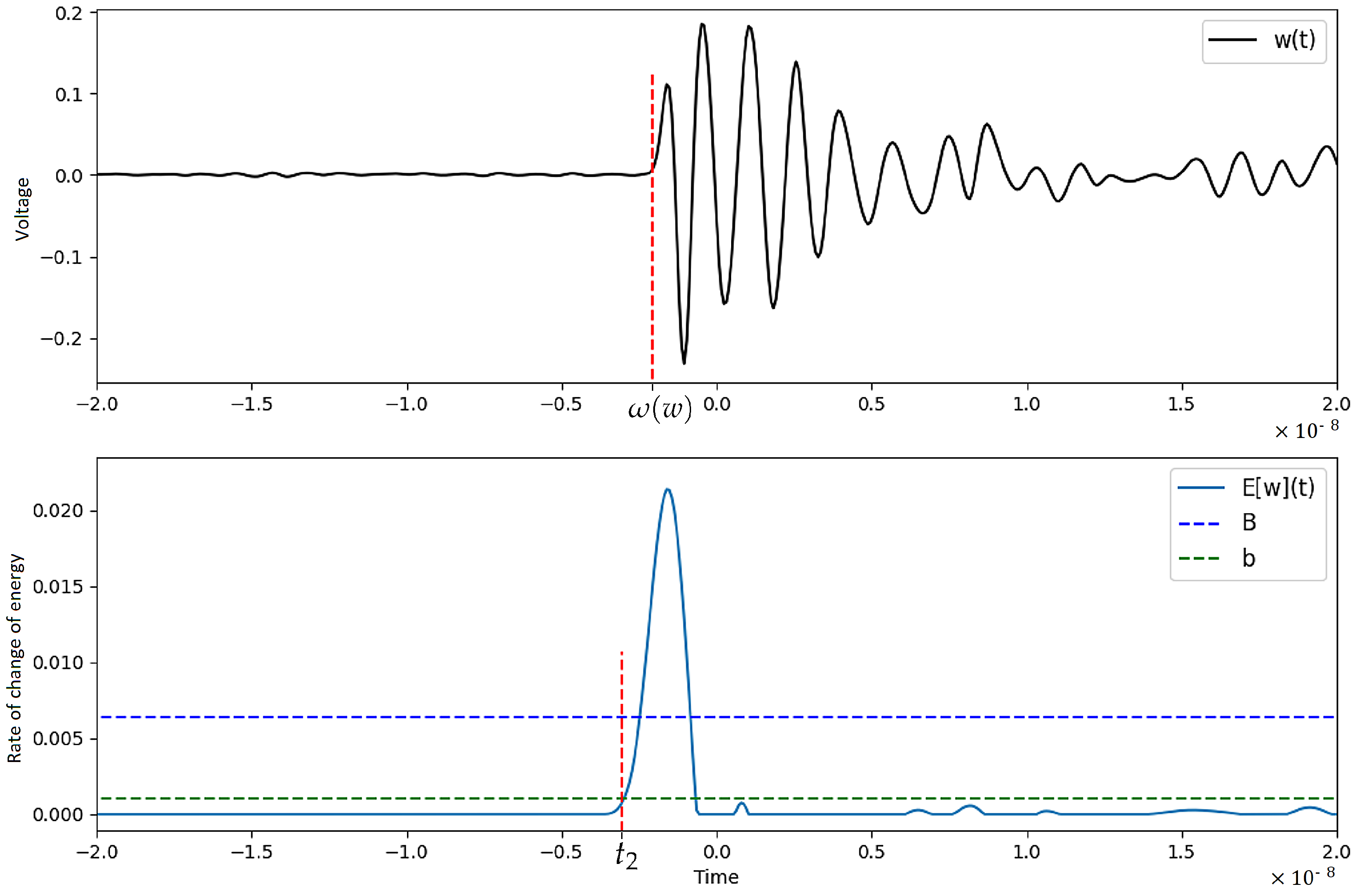
This function represents the rate of change of local energy content. As seen in Figure 1, an onset present in the signal $w\left(t\right)$ usually results in a peak in $E\left[w\right]$. The onset of $w\left(t\right)$ can then be identified as the time when the energy content of the signal begins to increase. In other words, the onset corresponds to the lowest point on the first peak identified in $E\left[w\right]$. We can locate this point using two thresholds and some simple criteria.

Given a signal $w\left(t\right)$, the algorithm used to find the onset $\omega \left(w\right)$ proceeds as follows:

• From $E\left[w\right]$, find upper and lower bounds $B=maxE\left[w\right]\left(t\right)/3$ and $b=maxE\left[w\right]\left(t\right)/20$.
• Find the earliest time $t_1$ for which $E\left[w\right]\left(t_1\right)\ge B$.
• Obtain $t_2$ by repeatedly decrementing $t_1$ by the sampling time $t_s$ until $E\left[w\right]\left(t_2\right)\le b$ and

  $$2E\left[w\right]\left(t_2\right)-E\left[w\right](t_2+t_s)>E\left[w\right](t_2-t_s)$$

  (3)
• Return $\omega \left(w\right)=t_2+T/4$.

The values chosen for the upper and lower bounds were found to work well in practice. The constant $T/4$ is used to compensate for the effect the window function width has on shifting the peak of $E\left[w\right]$.

This method has the added benefit of denoising the signal, as can be seen by how $E\left[w\right]$ is almost identically zero before the onset.

The window width T should be optimised to attain good selectivity while maintaining noise immunity. In practice, a value of $T=4$ ns was found to produce satisfactory results.

For signals $w_i\left(t\right),w_j\left(t\right)$, the time difference measurement ${\widehat{t}}_{i,j}$ is then given by

$${\widehat{t}}_{i,j}={\omega }_{i,j}+\underset{t\in [-ϵ,ϵ]}{argmax}{w}_i\ast w_j({\omega }_{i,j}+t)$$

(4)

where ${\omega }_{i,j}=\omega \left(w_i\right)-\omega \left(w_j\right)$ and $ϵ$ is the corelation window size.

This assumes that each signal measures the UHF radiation from one and only one discharge. Separate methods should be used for the detection and separation of UHF PD signals.

3. Location Estimation

Given four antennas with known locations $r_1,r_2,r_3,r_4$ and TDOAs $t_{i,j}$, the point of discharge x satisfies

$$\left\{\begin{array}{c}{d}_1-d_2=c·t_{1,2}\hfill \\ d_2-d_3=c·t_{2,3}\hfill \\ d_3-d_4=c·t_{3,4}\hfill \end{array}\right.$$

(5)

where $d_i=|x-r_i|$ and $c=3\times {10}^8$ is the speed of light in free space.

Closed-form solutions of (5) exist, assuming we have exact TDOAs [10]. Measurement noise causes acquired TDOA values ${\widehat{t}}_{i,j}$ to deviate from true values $t_{i,j}$. When noise is significant, closed-form solutions may produce significant errors or yield no roots altogether. In this section, we propose a minimum mean-squared-error (MMSE)-based location estimator that utilises prior knowledge of a substation’s layout.

We assume prior knowledge of potential PD locations, $x\in S\subset \mathrm{I}{\mathrm{R}}^3$. For simplicity, assume S is the union of disjoint cuboids.

$$S=\bigcup _{i=1}^n\underset{j=1}{\overset{3}{\times }}[a_{i,j},b_{i,j}]=\bigcup _{i=1}^n{S}_i$$

(6)

The measured TDOAs $\widehat{T}=[{\widehat{t}}_{1,2},{\widehat{t}}_{2,3},{\widehat{t}}_{3,4}]$ are assumed to be normally distributed with mean $T=[t_{1,2},t_{2,3},t_{3,4}]$ and covariance $\mathbf{\Sigma }$ given by

$$\begin{array}{c}\hfill \mathbf{\Sigma }=\left[\begin{array}{ccc}2{\sigma }^2& -{\sigma }^2& 0\\ -{\sigma }^2& 2{\sigma }^2& -{\sigma }^2\\ 0& -{\sigma }^2& 2{\sigma }^2\end{array}\right]\end{array}$$

(7)

assuming errors in onset detection are normally distributed with zero mean and variance ${\sigma }^2$.

The covariance calculation is reasonably accurate since the correlation term in (2) is usually much smaller than the onset term ${\omega }_{i,j}$ if $ϵ$ is small; therefore, we can assume that errors in $\widehat{T}$ result mostly from errors in onset detection.

For simplicity, we assume that the measurement noise ${\sigma }^2$ is fixed for all discharge and antenna positions. Given an antenna at point r and a point of discharge x, one would expect the noise ${\sigma }^2$ to increase with $|r-x|$ due to the reduction in UHF measurement SNR and depend on $\angle (r-x)$ through antenna directivity. In other words, we assume that the antennas $r_i$ are isotropic and neglect the dependence of UHF SNR on distance to antenna.

Given a measurement $\widehat{T}$, the posterior distribution is then given by

$$\begin{array}{c}\hfill p(x|\widehat{T})\propto I_S\left(x\right)·exp\left(-\frac{1}{2}\Delta T{\mathbf{\Sigma }}^{-1}\Delta T\right)\end{array}$$

(8)

where $\Delta T_i={\widehat{T}}_i-d_i+d_{i+1}$ and $I_S$ is the indicator function on S.

The Metropolis-Hastings algorithm is used to obtain samples $X_1,\dots ,X_l$ from distribution (8) [11]. The position estimator $\widehat{x}(\widehat{T})$ is obtained by first finding the region $S_m\subset S$ that contains the largest number of samples, then taking an average of the samples in that region,

$$\widehat{x}(\widehat{T})=\frac{1}{\left|J\right|}\sum _{i\in J}{X}_i$$

(9)

where $J=\{i:X_i\in S_m\}$.

This method ensures that $\widehat{x}\in S$ as the standard MMSE estimator $\mathbf{E}(x|\widehat{T})$ may yield estimates that are outside S.

4. Optimising Antenna Placement

Every antenna array placement has better location accuracy in certain directions than others. As we are looking for PD in S, the antenna array placement should be optimised to yield the best location accuracy in that region.

The Cramer–Rao lower bound (CRLB) provides a lower bound on the covariance of any unbiased estimator. The CRLB matrix for a TDOA position estimator is known to be

$$\begin{array}{c}\hfill \mathit{C}=c^2{\left(\mathit{U}{\mathbf{\Sigma }}^{-1}{\mathit{U}}^T\right)}^{-1}\end{array}$$

(10)

with

$$\begin{array}{cc}\hfill \mathit{U}& =\left[\begin{array}{c}{u}_1-u_2\\ u_2-u_3\\ u_3-u_4\end{array}\right]\hfill \end{array}$$

(11)

where $u_i=\frac{x-r_i}{d_i}$ is the unit vector from $r_i$ to x [7].

To maximise location accuracy in a region S, we look to find $\mathit{R}={\left[r_1{r}_2{r}_3{r}_4\right]}^T$, which minimises ${\int }_S\left|\mathit{C}\right|$ subject to constraints $|r_i|\le L$. This is equivalent to maximising ${\int }_S{\left|\mathit{U}\right|}^2$, which we do here.

A stochastic projected gradient (SPG) algorithm is used to solve this optimisation problem. An initial point ${\mathit{R}}_0$ satisfying problem constraints is chosen randomly, then repeatedly updated using the rule

$${\mathit{R}}_{n+1}=P\left({\mathit{R}}_n+\frac{\alpha }{N}\sum _{i=1}^N{\nabla }_R{\left|\mathit{U}\left(x_{i,n}\right)\right|}^2\left({\mathit{R}}_n\right)\right)$$

(12)

where $x_{i,j}\in S$ are resampled at every iteration. The function $P\left(\mathit{R}\right)={\left[P\left(r_1\right)P\left(r_2\right)P\left(r_3\right)P\left(r_4\right)\right]}^T$ projects every point onto the constraint region

$$P\left(r\right)=\left\{\begin{array}{c}r\left|r\right|\le L\hfill \\ \frac{Lr}{\left|r\right|}\left|r\right|>L\hfill \end{array}\right..$$

(13)

Using Jacobi’s formula to calculate the gradient yields

$$\begin{array}{cc}\hfill ({\nabla }_R{\left|\mathit{U}\left(x\right)\right|}^2{)}_{i,j}& =2\left|\mathit{U}\left(x\right)\right|·({\nabla }_R{\left|\mathit{U}\left(x\right)\right|)}_{i,j}\hfill \end{array}$$

(14)

$$\begin{array}{cc}\hfill & ={2\left|\mathit{U}\left(x\right)\right|}^2·tr\left({\mathit{U}}^{-1}·\frac{\partial \mathit{U}}{\partial {\mathit{R}}_{i,j}}\right)\hfill \end{array}$$

(15)

with

$$\begin{array}{cc}\hfill \frac{\partial \mathit{U}}{\partial {\mathit{R}}_{i,j}}& =\left[\begin{array}{c}{D}_{i,j}{u}_1-D_{i,j}{u}_2\\ D_{i,j}{u}_2-D_{i,j}{u}_3\\ D_{i,j}{u}_3-D_{i,j}{u}_4\end{array}\right]\hfill \end{array}$$

(16)

where $D_{i,j}{u}_k=\frac{{\delta }_{i,k}}{d_k}·Q_j(u_k^T{u}_k-I)$, $Q_j=[{\delta }_{1,j},{\delta }_{2,j},{\delta }_{3,j}]$, and ${\delta }_{i,k}$ is the Kronecker delta.

The above algorithm does not guarantee a global minimum of ${\int }_S\left|\mathit{C}\right|$, as the optimisation problem is non-convex. For more reliable results, the algorithm could be ran multiple times with different initial conditions before taking the best result.

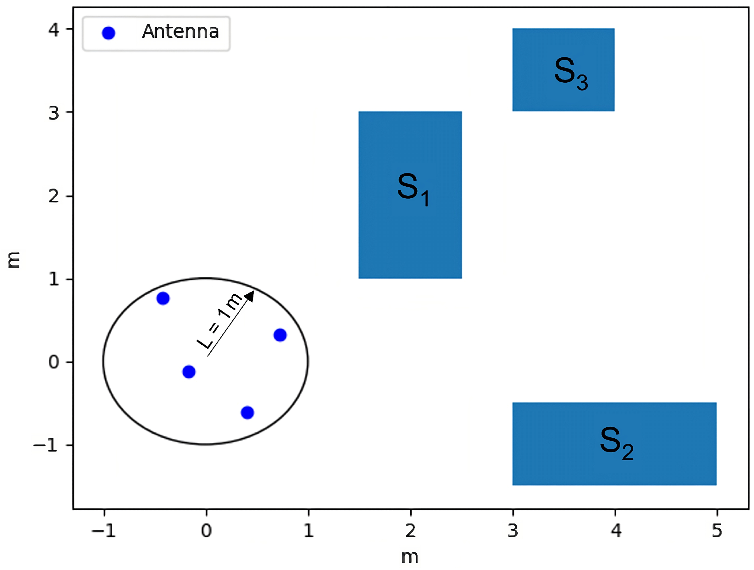
An example set S, along with its optimised antenna placements are shown in Figure 2.

5. Antenna Position Calibration

Obtaining accurate measurements of antenna positions $\mathit{R}$ while also maintaining a reasonable coordinate system (usually with the x–y plane parallel to the ground and the z-axis pointing to the sky) is difficult for all but the simplest antenna configurations. This is partially why many similar UHF PD location systems [12,13] resort to placing antennas in a rectangle despite the tetrahedron antenna placement being arguably more optimal [7]. To simplify this process, we propose a scheme for setting up a coordinate system and finding antenna positions in that system.

We assume that a portable source of UHF signals is available; this could, for example, be a piezoelectric discharge generator or an additional antenna with a signal generator. Aside from being used for the calibration procedure to follow, a portable UHF source could also be used for identifying the coordinates of any point in space, which would be helpful in mapping out the regions $S_i$.

The following steps are required for the calibration process:

• Obtain measurements $d_{i,j}=|r_i-r_j|$ of the distances between the antennas. This could be carried out manually using a tape measure or radiometrically by generating a signal from one antenna and finding the time of flight to other antennas.
• Place the UHF signal source at point $p_0$, which will act as the origin. Generate a signal from that point, which can then be measured by the antennas to obtain a set of 3 TDOA values using the onset algorithm.
• Place the UHF signal source at a point $p_1$ such that the vector $p_1-p_0$ points in the desired positive x direction. Obtain TDOA values as in 2.
• Place the UHF signal source at any point $p_2$ on the desired x–y plane such that its y-coordinate is positive. Obtain TDOA values.

From the measurements $d_i$, we can obtain an intermediate set of antenna positions,

$${\mathit{R}}_I=\left[\begin{array}{ccc}0& 0& 0\\ x_2& 0& 0\\ x_3& \sqrt{d_{1,3}^2-x_3^2}& 0\\ x_4& y_4& \sqrt{d_{1,4}^2-x_4^2-y_4^2}\end{array}\right]$$

(17)

where

$$\begin{array}{cc}\hfill x_i& =\frac{d_{1,i}^2-d_{2,i}^2+d_{1,2}^2}{2d_{1,2}}\hfill \end{array}$$

(18)

$$\begin{array}{cc}\hfill y_4& =\frac{d_{2,4}^2-d_{3,4}^2+{(x_4-x_3)}^2-{(x_4-x_2)}^2+d_{1,3}^2-x_3^2}{2\sqrt{d_{1,3}^2-x_3^2}}\hfill \end{array}$$

(19)

It can be shown that antenna positions ${\mathit{R}}_I$ satisfy the measurements $d_{i,j}$.

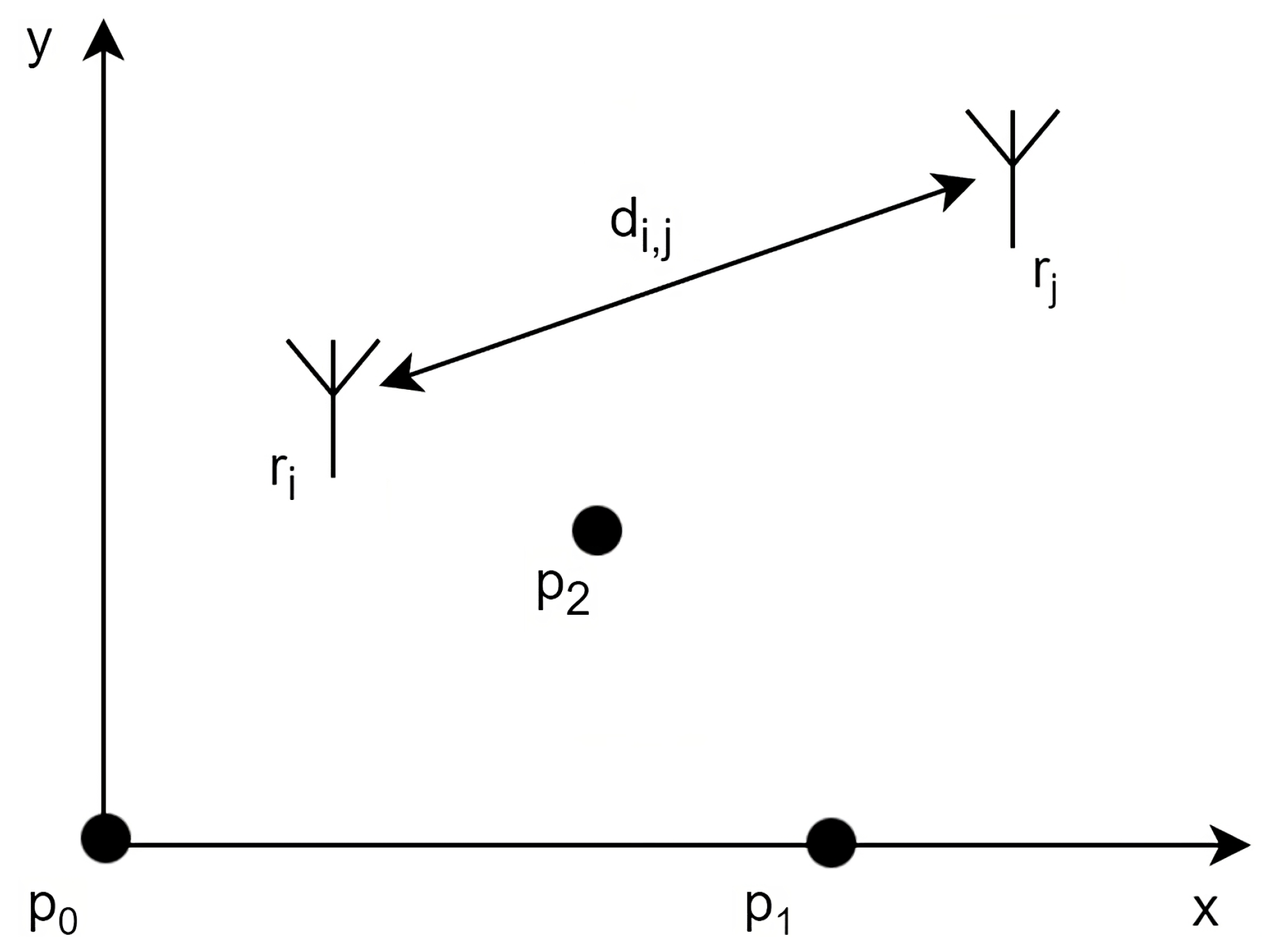
Using the TDOA measurements acquired, the positions of points $p_i$ in the intermediate coordinate system can be deduced. The desired coordinate system has the points $p_i$, as shown in Figure 3. We can then define a distance-preserving transformation, T, which takes the intermediate system to the desired one. The transformation T is given by

$$T\left(x\right)=R_2{R}_1(x-p_0)$$

(20)

with

$$\begin{array}{c}\hfill \begin{array}{cc}\hfill R_i& ={\left(w_i\right)}_{i}I-{\left[v_i\right]}_{\times }+\frac{1-{\left(w_i\right)}_i}{|v_i{|}^2}\left(v_i^T{v}_i\right)\hfill \\ \hfill v_i& =w_i\times Q_i\hfill \\ \hfill w_1& =p_{1,0}/\left|p_{1,0}\right|\hfill \\ \hfill w_2& =h/\left|h\right|,h=[0,R_1{\left(p_{2,0}\right)}_2,R_1{\left(p_{2,0}\right)}_3]\hfill \end{array}\end{array}$$

(21)

where $p_{i,j}=p_i-p_j$ and ${\left[v\right]}_{\times }$ is the cross-product matrix of v.

The antenna positions $\mathit{R}$ in the desired coordinate system are then given by

$$\mathit{R}=T\left({\mathit{R}}_I\right)$$

(22)

with the understanding that T acts on ${\mathit{R}}_I$ in a row-wise fashion.

When compared with the more intuitive method of finding antenna positions by measuring lengths in orthogonal directions, the proposed method uses only antenna-to-antenna measurements, which are simpler to acquire in practice.

6. Results

A combination of experimental and simulation results were used to compare the methods presented in this paper with other popular techniques.

6.1. Simulation Results

A simulation of random PDs in a 10 m × 10 m × 10 m region with $L=1$ m was carried out, with the antennas placed in the centre of the cube region. The regions $S_i$ were randomly chosen with random side lengths in the range $0<b_{i,j}-a_{i,j}<2$. Monte Carlo trials were used to estimate the average localization errors for every substation layout S. These errors were then averaged over multiple random layouts to obtain an overall average.

Two simulations were conducted, including one for comparing location estimators and another for studying the performance of the SPG algorithm.

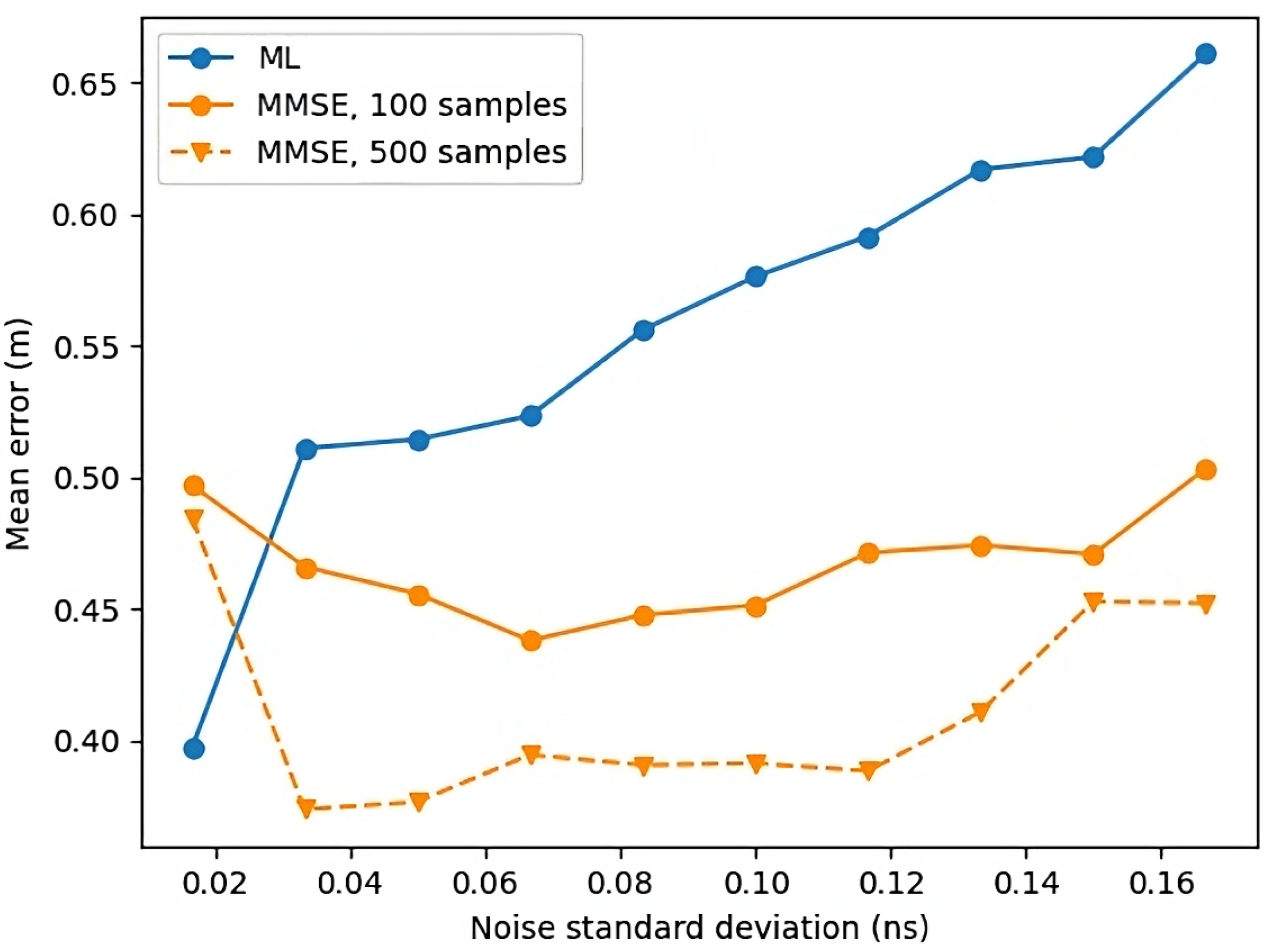
Maximum likelihood (ML) estimators are the most common type of location estimators [14,15]. We compared the MMSE location estimator presented in Section 3 with a maximum likelihood estimator restricted over the set S

$${\widehat{x}}_{ML}(\widehat{T})=\underset{x\in S}{argmax}p(x|\widehat{T}).$$

(23)

The ML estimate was computed using gradient ascent. The algorithm was carried out once for every region $S_i$ using an initial condition from that region. Of those solutions, the one that maximized the posterior distribution was chosen as the location estimate.

As shown in Figure 4, the MMSE estimator outperforms the ML estimator by a significant margin for large values of $\sigma$. Increasing the number of samples used for the MMSE estimator increases accuracy by bringing the calculated region average closer to the true average. For small values of $\sigma$, the distribution (8) has a sharper peak, which the sampling algorithm fails to accurately represent, resulting in poor MMSE accuracy.

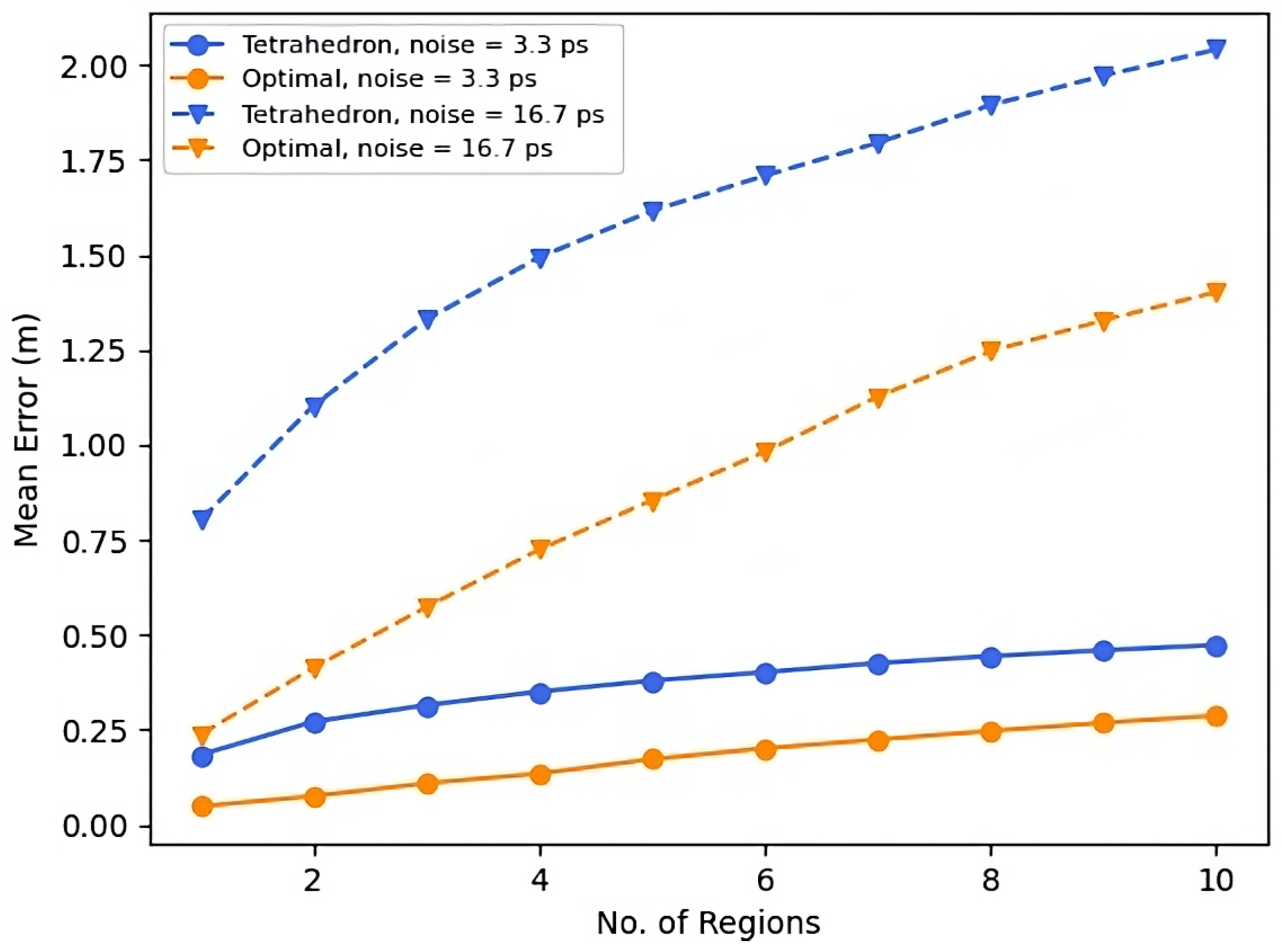
It is known that placing antennas as the vertices of a tetrahedron maximises the trace of the FIM at the centre of the tetrahedron [7]. We compare the performance of configurations given by the SPG algorithm to the tetrahedron placement with vertices on the unit sphere.

The location estimator used is a version of the closed-form solution given in [10], which has been adapted for the problem in (5). Unlike the ML or MMSE estimators used above, the closed-form solution has no upper bound on localization errors for a given substation, which results in some position estimates with anomalously large errors. To minimise this effect, we use the median error for a layout instead of the mean.

Optimal arrays were obtained by running the SPG algorithm three times and taking the best result.

As shown in Figure 5, the optimal configurations obtained from the SPG algorithm were consistently better than the tetrahedron configuration. The dependence of tetrahedron configuration errors on the number of regions is due to how roots of (5) were chosen.

6.2. Experimental Results

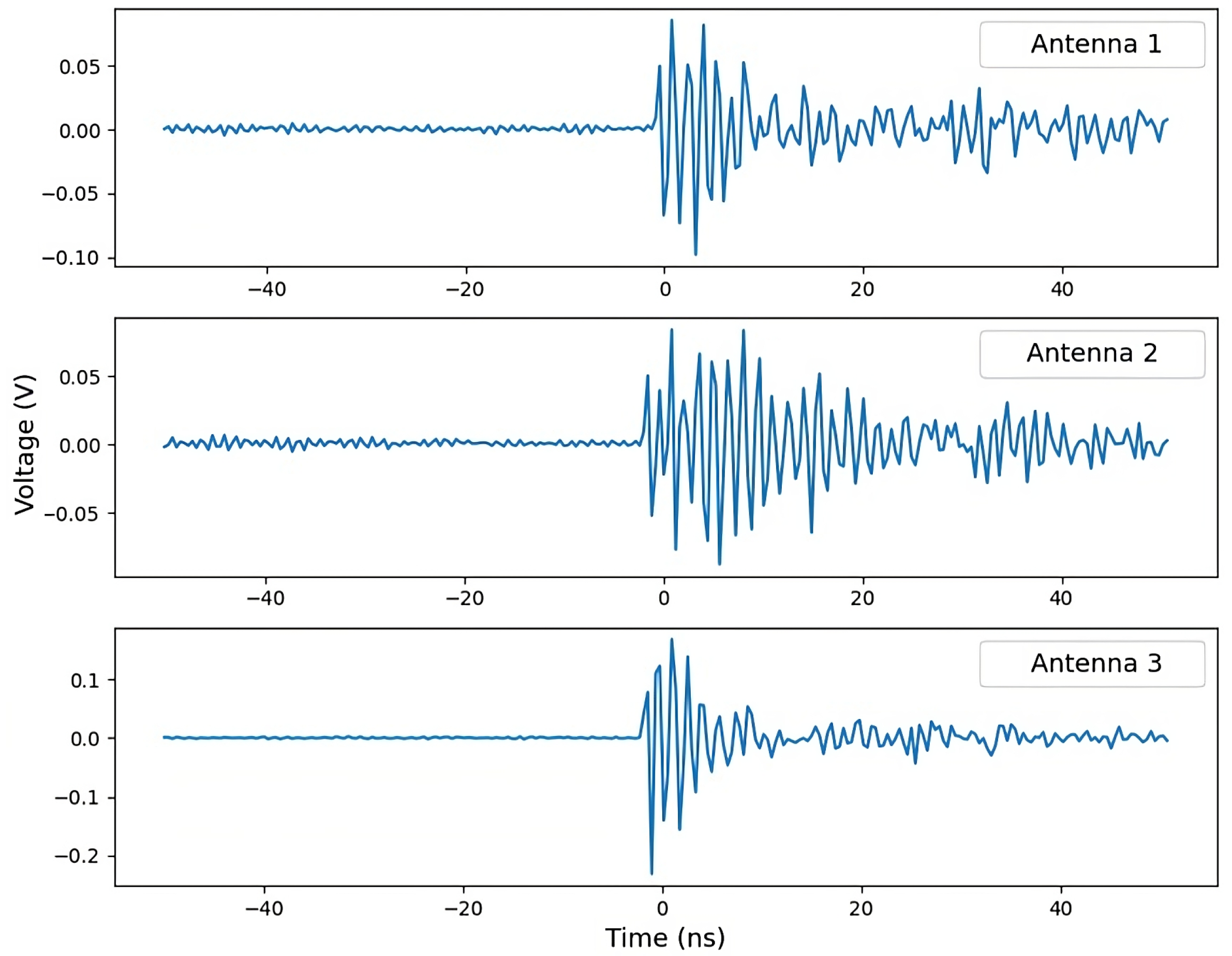
A piezoelectric discharge generator was used generate EM radiation in the frequency range typically emitted by a partial discharge. These data were captured on a 1 GHz, 2.5 GS/s oscilloscope, which was connected, using equal length coaxial cables, to a set of 3 monopole antennas with a high sensitivity in the UHF range. These waveforms were then used to compare the method described in Section 2 to other common methods of obtaining TDOA measurements. A typical UHF measurement is shown in Figure 6.

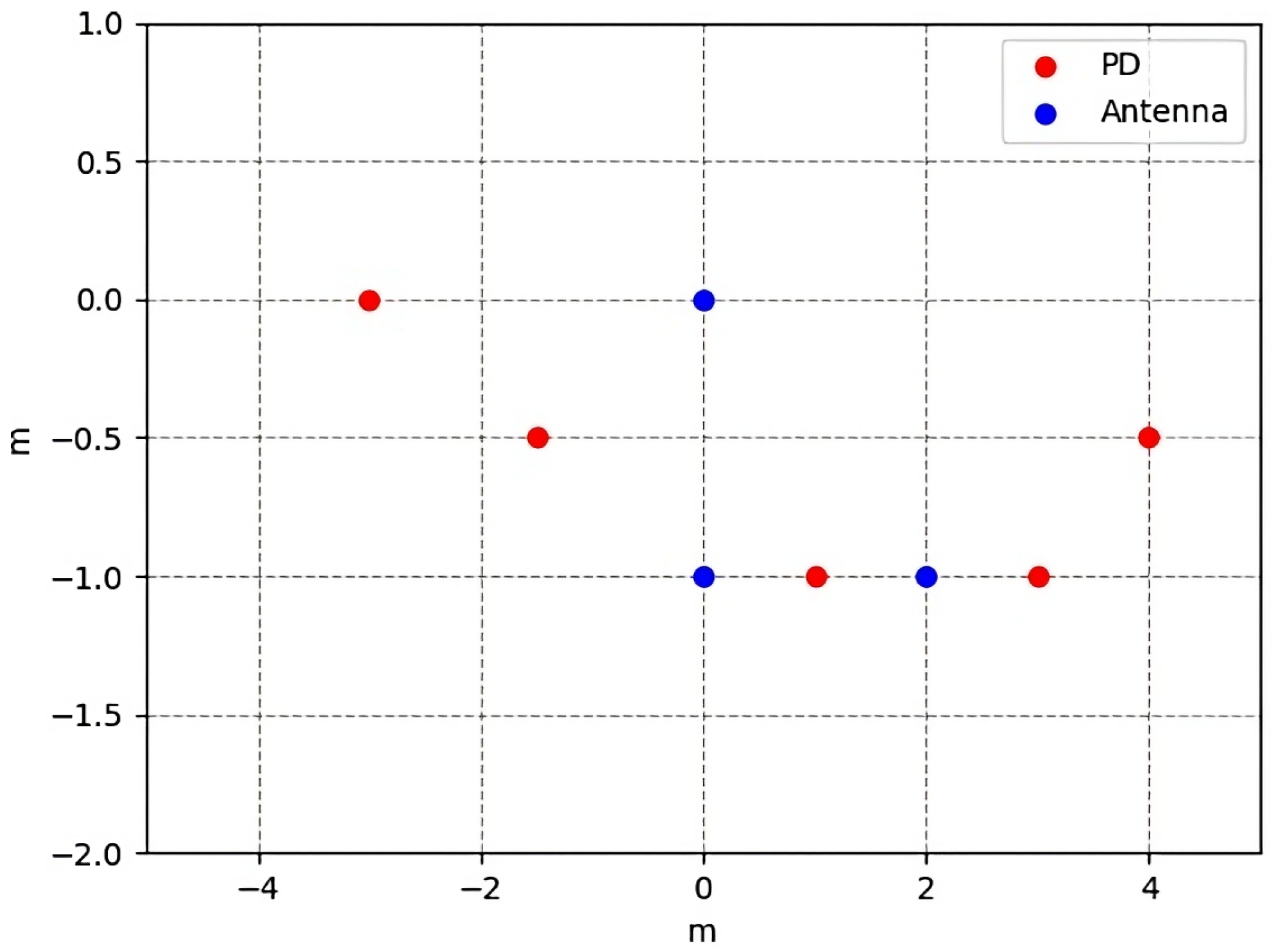
As is shown in Figure 7, three antennas were placed in positions (0,0), (0,−1), and (2,−1). PDs were placed in positions (1,−1), (3,−1), (−1.5,−0.5), (4,−0.5), and (−3,0). Both antenna and PD positions were placed at a fixed height such that they were all coplanar. For every discharge, two time difference measurements were taken. Measurements with an error larger than $5$ ns between the two time difference values were discarded.

Besides the algorithm presented in Section 2, the following time delay estimation algorithms were used:

• Onset: Similar to (4) but without the correlation stage, i.e., ${\widehat{t}}_{i,j}={\omega }_{i,j}$
• Denoise + First peak: Applies wavelet denoising, then takes the difference between first peaks [5].
• Threshold: Difference between the earliest times that go above the threshold $max\left|w\right(t\left)\right|/4$.
• Correlation: ${\widehat{t}}_{i,j}=\underset{t}{arg\; max}{w}_i\ast w_j\left(t\right)$.

The two onset algorithms were proposed in this paper. The other three estimators are commonly used in similar systems.

All signals were 5× upsampled using cubic splines before being passed to a time delay estimator.

The results in

Table 1. Mean error for different time delay estimation algorithms. The onset techniques (in bold) were proposed in this paper.

Algorithm	Error (ns)
Onset + Correlation	0.16
Onset	0.24
Denoise + First peak	0.44
Threshold	0.55
Correlation	1.19

show that the denoise + first peak method outperforms signal correlation, which is in agreement with what was reported in [5]. The onset techniques provide a significant improvement in accuracy over the other algorithms. A window size of $ϵ=1.2$ ns was used for the onset + correlation algorithm. Larger values of $ϵ$ tended to perform worse than the regular onset algorithm.

7. Case Study

The main downside to the techniques presented here is their dependence on certain prior information. The SPG algorithm requires prior knowledge of the set S, and the location estimator $\widehat{x}(\widehat{T})$ requires knowledge of both S and the noise statistic $\sigma$. The set S would have to be determined through substation measurements, while $\sigma$ could either be estimated empirically, as occurred in Table 1, or deduced by fitting the measured data to a clustering model, similar to what occurred in [16].

To justify the additional demands of these methods, we compared the system proposed in this paper with a more conventional system that does not require the prior information mentioned above.

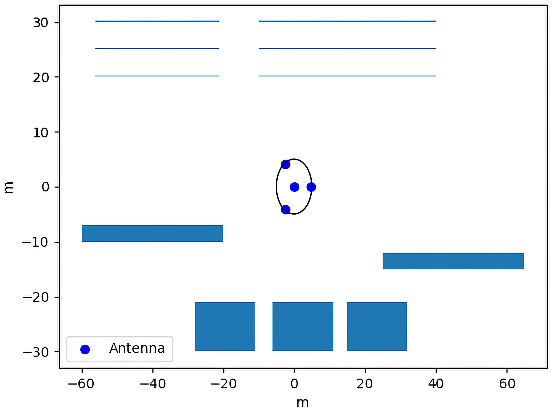
The layout S used in this case study is shown in Figure 8; it is based on the dimensions of regions occupied by electrical plant items in an open-air substation in the UK. Antennas are restricted to a sphere of radius $L=5$ m. For simplicity, line-of-sight considerations are neglected.

The conventional system used here consists of the closed-form location estimator in [10] with a tetrahedral antenna placement. The proposed system uses the MMSE estimator (9), with antenna placements given by the SPG algorithm.

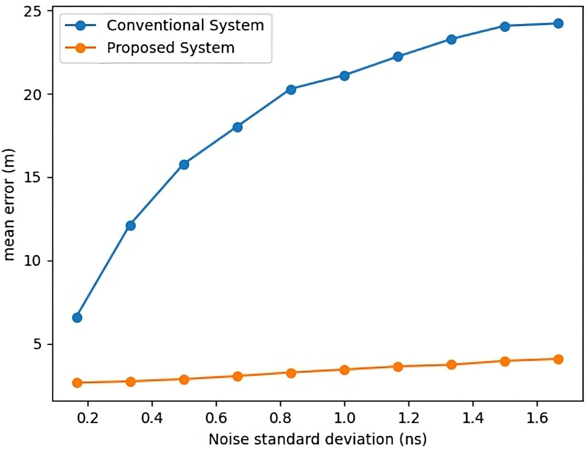
As in Section 6, results were gathered using Monte Carlo trials. Mean error values were obtained by averaging the median square error for a set of simulated PDs over different antenna configurations given by the SPG algorithm.

As could be seen in Figure 9, the combination of both the SPG algorithm and the MMSE location estimator result in significant improvements in location accuracy. For the noise range shown, the conventional system is, on average, 4.5 times less accurate than the proposed system, with a maximum error 5.9 times greater for the highest noise simulation.

Areas occupied by HV equipment are typically inhomogeneous. This means that the point of discharge no longer satisfies Equation (5), so estimates of position inside HV equipment are very unreliable. Due to this, identifying which piece of equipment contains the fault might be more relevant than looking at absolute errors in localization.

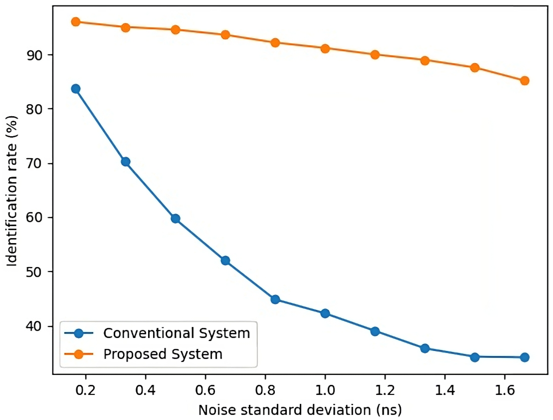
The problem of equipment identification may be modelled as the identification of the discharge region $S_i$, which contains the PD. From the MMSE estimator (9), the discharge region could be estimated to be the region $S_m$, which contains the largest number of PD samples drawn. For conventional location estimators, the discharge region is estimated as the region closest to the PD position calculated.

Using these estimates, we can find the rate of discharge region identification for both systems.

As seen in Figure 10, the proposed system again outperforms the conventional system with an average identification rate 42% higher over the noise range shown.

8. Conclusions and Future Work

The onset-based TDOA estimator presented here has been shown to be more than twice as accurate as other established techniques.

By utilising prior knowledge of substation layout, we developed an MMSE-based location estimator that yields more accurate estimates than the commonly used maximum likelihood estimator in high-noise situations. The antenna placements given by the SPG algorithm presented were shown to be consistently more accurate than the tetrahedron antenna placement and provided a more significant improvement in accuracy when the measurement noise was high. Combining the MMSE-based estimator and the optimised antenna placement resulted in a system that was 5.9 times more accurate than a conventional system in the highest measurement noise simulation conducted. This improvement in accuracy might justify the additional prior information required by the methods presented here. If this is the case, it can lead the way for more accurate fault localization systems that can utilise the geometry of their surrounding environment.

To simplify the problem of PD location, we assumed that all antennas had a line of sight to the point of discharge and neglected the dependence of measurement noise on antenna and discharge positions. Future work could look to include these effects in the problem formulated in Section 3 to potentially derive better methods for PD positioning and antenna placement. Additional research could also look to use UHF signal strength measurements to aid in PD positioning.

References

- Xavier, G.V.R.; Silva, H.S.; da Costa, E.G.; Serres, A.J.R.; Carvalho, N.B.; Oliveira, A.S.R. Detection, Classification and Location of Sources of Partial Discharges Using the Radiometric Method: Trends, Challenges and Open Issues. IEEE Access 2021, 9, 110787–110810. [Google Scholar] [CrossRef]
- Masaki, K.; Sakakibara, T.; Murase, H.; Akazaki, M.; Uehara, K.; Menju, S. On-site measurement for the development of on-line partial discharge monitoring system in GIS. IEEE Trans. Power Deliv. 1994, 9, 805–810. [Google Scholar] [CrossRef]
- Pearson, J.S.; Farish, O.; Hampton, B.F.; Judd, M.D.; Templeton, D.; Pryor, B.W.; Welch, I.M. Partial discharge diagnostics for gas insulated substations. IEEE Trans. Dielectr. Electr. Insul. 1995, 2, 893–905. [Google Scholar] [CrossRef]
- Mashikian, M.S. Preventive maintenance testing of shielded power cable systems. IEEE Trans. Ind. Appl. 2002, 38, 736–743. [Google Scholar] [CrossRef]
- Sinaga, H.H.; Phung, B.T.; Blackburn, T.R. Partial discharge localization in transformers using UHF detection method. IEEE Trans. Dielectr. Electr. Insul. 2012, 19, 1891–1900. [Google Scholar] [CrossRef]
- Moore, P.J.; Portugues, I.E.; Glover, I.A. Radiometric location of partial discharge sources on energized high-Voltage plant. IEEE Trans. Power Deliv. 2005, 20, 2264–2272. [Google Scholar] [CrossRef]
- Yang, B.; Scheuing, J. Cramer-Rao bound and optimum sensor array for source localization from time differences of arrival. In Proceedings of the ICASSP ’05, IEEE International Conference on Acoustics, Speech, and Signal Processing, Philadelphia, PA, USA, 18–23 March 2005; Volume 4, pp. iv/961–iv/964. [Google Scholar] [CrossRef]
- Bishop, A.N.; Fidan, B.; Anderson, B.D.O.; Pathirana, P.N.; Dogancay, K. Optimality Analysis of Sensor-Target Geometries in Passive Localization: Part 2—Time-of-Arrival Based Localization. In Proceedings of the 2007 3rd International Conference on Intelligent Sensors, Sensor Networks and Information, Melbourne, VIC, Australia, 7–10 December 2007; pp. 13–18. [Google Scholar] [CrossRef]
- Müller, M. Fundamentals of Music Processing: Audio, Analysis, Algorithms, Applications, 1st ed.; Springer: Berlin/Heidelberg, Germany, 2015; pp. 306–309. [Google Scholar]
- Bancroft, S. An Algebraic Solution of the GPS Equations. IEEE Trans. Aerosp. Electron. Syst. 1985, AES-21, 56–59. [Google Scholar] [CrossRef]
- Luengo, D.; Martino, L.; Bugallo, M.; Elvira, V.; Särkkä, S. A survey of Monte Carlo methods for parameter estimation. EURASIP J. Adv. Signal Process. 2020, 2020, 25. [Google Scholar] [CrossRef]
- Zhu, M.-X.; Yao, B.; Liu, Q.; Zhang, J.; Deng, J.; Zhang, G.; Shao, X.; He, W. Localization of multiple partial discharge sources in air-insulated substation using probability-based algorithm. IEEE Trans. Dielectr. Electr. Insul. 2017, 24, 157–166. [Google Scholar] [CrossRef]
- Portugues, I.E.; Moore, P.J.; Glover, I.A.; Johnstone, C.; McKosky, R.H.; Goff, M.B.; van der Zel, L. RF-Based Partial Discharge Early Warning System for Air-Insulated Substations. IEEE Trans. Power Deliv. 2009, 24, 20–29. [Google Scholar] [CrossRef]
- Chan, Y.T.; Ho, K.C. A simple and efficient estimator for hyperbolic location. IEEE Trans. Signal Process. 1994, 42, 1905–1915. [Google Scholar] [CrossRef]
- Jin, B.; Xu, X.; Zhang, T. Robust Time-Difference-of-Arrival (TDOA) Localization Using Weighted Least Squares with Cone Tangent Plane Constraint. Sensors 2018, 18, 778. [Google Scholar] [CrossRef] [PubMed]
- Mishra, D.K.; Sarkar, B.; Koley, C.; Roy, N.K. An unsupervised Gaussian mixer model for detection and localization of partial discharge sources using RF sensors. IEEE Trans. Dielectr. Electr. Insul. 2017, 24, 2589–2598. [Google Scholar] [CrossRef]
Figure 1.
Graphical representation of the onset algorithm. (Top) Discharge UHF measurement. (Bottom) with upper and lower thresholds used for peak finding.
Figure 2.
Overhead plot of an example set S along with its optimised antenna placement as given by the SPG algorithm.
Figure 3.
Graphical representation of measurements required for calibration.
Figure 4.
Localization errors of ML and MMSE estimators as functions of noise.
Figure 5.
Localization errors of tetrahedron and optimal antenna placements as a function of the number of regions for two different values of noise standard deviation.
Figure 6.
Typical UHF measurements for one PD.
Figure 7.
Antenna and artificial PD locations for experimental verification of time delay estimation algorithm.
Figure 8.
Substation layout used for case study. The blue regions represent the set S from which PD can emanate.
Figure 9.
Mean localization error as function of noise for the two systems under study.
Figure 10.
Discharge region identification rate as a function of noise for the two systems under study.