
An Unmanned Helicopter Energy Consumption Analysis
by
 , ,
, ,
Marcin Żugaj
1,*, 
Mohammed Edawdi
1,
Grzegorz Iwański
2,
Sebastian Topczewski
1,
Przemysław Bibik
1 and
Piotr Fabiański
2 1
Faculty of Power and Aeronautical Engineering, Warsaw University of Technology, St. Nowowiejska 24, 00-665 Warsaw, Poland
2
Faculty of Electrical Engineering, Warsaw University of Technology, St. Koszykowa 75, 00-662 Warsaw, Poland
*
Author to whom correspondence should be addressed.
Energies 2023, 16(4), 2067; https://doi.org/10.3390/en16042067
Submission received: 20 January 2023
/
Revised: 6 February 2023
/
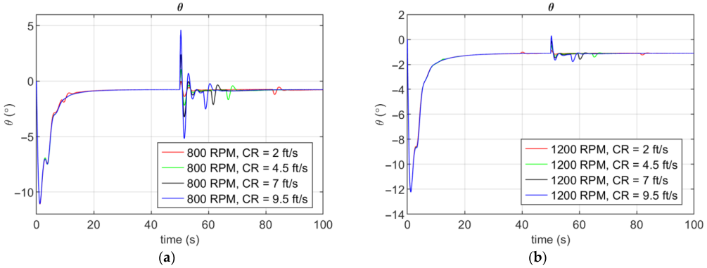
Accepted: 8 February 2023
/
Published: 20 February 2023
(This article belongs to the Special Issue Modeling for Energy Consumption Analysis)
Abstract
:The number of operations incorporating E-VTOL aircrafts is increasing each year, and the optimization of the energy consumption of such vehicles is a major problem. In this paper, a small-scale ARCHER helicopter’s energy consumption is analyzed, wherein different flight conditions, main rotor revolutions, and flight control system settings are considered. The helicopter dynamic model was developed in the FLIGHTLAB environment and was then validated based on flight test data. The model used for the calculation of energy consumption was developed using the electric and dynamic characteristics of the main rotor, electric motor, and transmission system. The main part of this work concerns the analysis of electric energy consumption during the vehicle’s flight via the use of an automatic flight control system (AFCS) that ensures repeatable flight conditions. The AFCS was designed such that it includes both path and attitude control to provide hover and cruise control modes. The helicopter’s energy consumption was analyzed during different phases of flight, when executing maneuvers, and using different main rotor angular velocities to perform - a given task. The results show that the level of energy consumption significantly depends on the helicopter’s main rotor revolutions, flight speed, and the maneuvers performed. The proposed methodology can be used in prospective energy-efficient mission planning and UAV helicopter design.
1. Introduction
The number and complexity of Unmanned Aerial Vehicles (UAV)-based operations are increasing each year. Electric Vertical Take-off and Landing (E-VTOL) aircrafts constitute a large group of flying vehicles. Such vehicles are capable of vertical take-off and landing, hovering, and performing precise, slow maneuvers, which gives them an advantage over fixed wing aircraft. However, the efficiency of energy consumption for such systems is significantly lower. Therefore, the problem of energy consumption optimization is of interest to research centers around the world [1,2,3,4,5]. The most popular E-VTOL configuration is a quadcopter because of its relative simplicity to design, build, and control [6,7]; therefore, this configuration most often appears in the research results concerning E-VTOL energy consumption [8,9,10,11,12,13,14,15,16,17,18,19,20,21,22,23] focusing on physics-based and experiment-based energy consumption models. There is a research niche in the field of energy consumption optimization concerning a small group of E-VTOL systems designed as helicopters. Due to their design, these vehicles’ levels of energy consumption are high, and control is quite complicated compared to other types of rotorcrafts such as quadcopters. However, their design enables the construction of both a micro- and macro-sized rotorcraft in terms of the carried payload, which gives them a definite advantage over other types of rotorcrafts. Currently, many studies related to helicopters are being conducted by helicopter companies and research institutions. The objective of such research is the improvement of helicopters’ flight performance via the optimization of rotor characteristics, the minimization of energy consumption, and the introduction of new helicopter configurations, i.e., compound helicopters (with additional lifting surfaces and propellers) [24,25,26,27,28,29,30,31,32,33,34]. Most of these studies address micro electric and macro non-electric helicopters. There is a lack of research results related to small-scale electric helicopters in the literature. Therefore, research programs addressing small electric helicopters of the classic configuration have been established at the Warsaw University of Technology. One of these is aimed at energy consumption analysis, which can be helpful in the design of a helicopter in terms of improving flight characteristics such as range, flight duration, and payload. In the classic configuration, the main and tail rotors are powered by electric motors, which provide lift, thrust, and control of the helicopter, resulting in a significant usage of electric power. In addition, all of the onboard systems are usually electric-powered. In a classic (non-hybrid) electrically powered helicopter, the only source of energy is a battery. So, the helicopter’s performance can be improved by optimizing energy management and the operation of the electric motor and the entire power system. Therefore, from the point of view of mission efficiency and duration, the optimization of helicopter energy consumption is an important task [35,36] and constitutes part of the worldwide trend of building green aircraft.
A helicopter is an aircraft whose flight is enabled by controlling the vectors of forces and moments generated by the main and tail rotors at a constant rotation speed or RPM (revolutions per minute). Such a design facilitates the construction of aircraft with VTOL characteristics of a greater weight and size than in the case of a multirotor configuration such as a quadrotor [37]. In UAV helicopters, both the flight and energy characteristics depend on the efficiency of the rotor set and the electric motor. The RPM of the main rotor is a factor that has a major impact on the flight and control characteristics of the helicopter and the energy consumption during steady flight and maneuvering. An appropriate value of the RPM can contribute to the efficient use of energy stored on board the helicopter and thus to its effective use. However, it should be noted that the variation of the RPM also affects flight characteristics and control characteristics, which may impede the performance of a particular flight task. Therefore, it is necessary to study the effect of the RPM of the main rotor on the energy use and control performance of the helicopter during typical flight phases and maneuvers [38]. Thus, a complex mathematical model of a helicopter that considers the dynamic characteristics of the rotor set, the propulsion system, and the fuselage needs to be developed. It is also important to design an automatic flight control system that will enable the performance of simulation tests in selected flight states of the helicopter.
The method and comprehensiveness of helicopter motion modelling depend on requirements that are based on the purpose for which the helicopter model will be used [39]. In this regard, the helicopter model is designed to analyze the helicopter’s motion (flight dynamics), its energy consumption, and applied control laws. To obtain a high trust level (reliability) of the model, the dynamic, aerodynamic, and kinematic properties of the modelled helicopter (which can generally be divided into fuselage, rotors, empennage, engine, transmission, control system, and landing gear) have to be taken into account based on accurate helicopter characteristics (geometric, inertial, and aerodynamic) [40]. The reliability of the designed helicopter model depends on its proper validation, which is usually performed by comparing the simulation and flight tests results. Apart from in-house helicopter models, usually, two rotorcraft modelling environments are used: CAMRAD and FLIGHTLAB.
The modelling of UAV electric propulsion systems’ energy consumption and this parameter’s optimization constitute an important research topic [41,42]. In general, UAV electric propulsion systems comprise a source of power, an electric drive, and a propeller (rotor). UAV helicopters are additionally equipped with a transmission system. The manner of an electric propulsion system’s optimization depends on the task for which it is needed (e.g., the design parameters, cost, or mission parameters) [43,44,45,46,47]. While for the vast majority of multi-copter systems control is achieved by changing solely the angular velocities of the rotors, helicopters are designed to change both the angular velocities of their rotors and the blade pitch angles, which influences the characteristics of the rotors’ energy consumption [48,49,50,51]. Moreover, the minimum-power operating point of a rotor and the point of maximum transmission efficiency are divergent, and the points of minimum fuel consumption and minimum mechanical power are not met at the same operating point [52]. Therefore, a reliable energy consumption model of a helicopter propulsion system is needed to analyze a helicopter’s energy consumption during different flight tasks.
A UAV helicopter requires the use of an automatic flight control system that ensures stable flight along a planned route. During a typical flight route, two typical flight phases and three maneuvers can be distinguished. The two main flight phases are hovering at a constant altitude and cruise flying at a constant speed and altitude. The typical maneuvers are acceleration, climb, and banked (coordinated) turns. In order to conduct simulation tests in these flight states, an automatic control system has been developed. Its control laws were designed for a single RPM value. It is also possible to use adaptive control laws to obtain the optimal system settings for any RPM value. However, due to the objectives of this research, it was decided not to use such laws. This approach will facilitate a more accurate analysis of the degradation of the control characteristics caused by RPM variation.
The aim of the present work is to analyze the energy efficiency of a UAV helicopter. A six-degree-of-freedom nonlinear model of the electric-powered ARCHER helicopter with a dedicated electrical energy consumption model is used to analyze the energy consumption during different flight conditions, main rotor RPM values, and flight control system settings. The energy consumption of the electric motor of the main rotor is the subject of this work because it is the main consumer of electrical energy. This system is mainly responsible for generating the aerodynamic forces and moments needed for a helicopter’s flight and control. The helicopter model was built using the FLIGHTLAB software and validated during flight tests. A dedicated automatic flight control system (AFCS) was developed in the MATLAB/Simulink environments to simulate the helicopter missions in a repeatable way, thereby enabling the benchmarking of energy consumption. The results show that reducing the RPM value results in a decrease in energy consumption up to about 20% relative to the nominal value. However, this results in a significant degradation in control performance. For small RPM values, steady horizontal flight is possible but turning is problematic. In contrast, increasing the value of the RPM does not affect the control performance but increases energy consumption. In addition, the increase in energy consumption during a maneuver depends mainly on its duration. So, each maneuver requires additional energy compared to steady state flight. The presented results are an important contribution to the development of small, unmanned helicopters and to research on optimizing their energy consumption. Such helicopters can be used both in mission planning and in the design of new helicopters. The presented energy consumption model and the method of its development can be successfully used in the design of electric propulsion systems for a single-rotor helicopter of the classic configuration.
The organization of the paper is as follows. In Section 2.1, the ARCHER helicopter’s numerical model, which was developed using the FLIGHTLAB software, is described. In Section 2.2, the model of electrical energy consumption is presented. In Section 2.3, the AFCS is described in detail. Then, in Section 3, test cases showing the energy consumption of the ARCHER helicopter during different flight conditions are analyzed. The paper ends with conclusions and a description of future research.
2. Helicopter Simulation Model
2.1. Overview
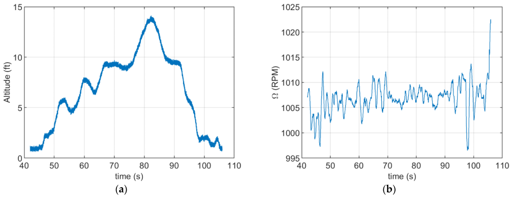
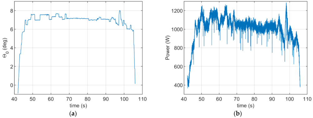
The analysis of the energy consumption of the helicopter used in this study required a sophisticated and reliable simulation environment that enables flight simulation according to various flight conditions and helicopter settings. Therefore, a simulation testbed was created based on two simulation programs: FLIGHTLAB version 3.7.1, which was released in 2020, and MATLAB/Simulink version 2017. First, the helicopter simulation model was developed in FLIGHTLAB. The model data were prepared based on a real helicopter’s design and flight dynamic calculations. Next, an Automatic Flight Control system was developed and programmed using the Simulink software. It also was optimized for a nominal value of RPM. Both FLIGHTLAB and Simulink were combined to create one advanced simulation environment. Finally, an energetic model of the electric engine with a whole power train was developed using a dedicated electric motor and gearbox, and it was implemented in the Simulink part of this testbed. The designed simulation model was tested and validated on two levels. The energy consumption model was designed and validated using a dedicated laboratory stand and the helicopter model was validated using the flight test results. Examples of the flight test results are shown in Figure 1 and Figure 2. These charts present the main rotor angular velocity , altitude, main rotor collective pitch angle , and electric power. The test was performed according to a main rotor angular velocity of 1000 RPM and a total helicopter mass (the mass of the helicopter and measurement system) of 9.11 kg. The data were affected by measurement noise and external disturbances. Data processing for parameter estimation was performed for hover conditions between 68 and 81 s of flight. The flight test results and values calculated by the simulation model are compared in Table 1. The difference between the simulation model and the real helicopter does not exceed 4%. This shows the adequacy of the model.
2.2. Archer Helicopter Numerical Model
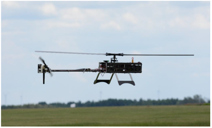
For the purpose of this research, the classic configuration, reconfigurable, and electric-powered ARCHER (Autonomous Reconfigurable Compound Helicopter for Education and Research) helicopter is used (Figure 3) [53]. ARCHER has two (main and tail) rotors with variable angular velocities and collective pitch angles of the blades, which are powered by two independent brushless electric motors connected to a lithium-polymer battery. All of the helicopter rotorhubs are rigid, with no flapping allowed. The helicopter was designed according to a constant nominal value of the main rotor RPM of 1000 and a cruise velocity of 34 ft/s. The basic parameters of the helicopter are shown in Table 2.
An ARCHER numerical model was developed in the FLIGHTLAB software, which is designed for the modelling of rotorcraft dynamics. All of the necessary mass-related, geometric, and aerodynamic parameters of the helicopter were included in the model. Blade element theory with quasi-steady aerodynamic loads (with stall regions characteristics included) and Peters–He six state inflow were used to model the main rotor. The aerodynamic characteristics of the blades’ airfoils were calculated using a CFD model and validated based on the flight test data. The tail rotor was modelled as a disc to make the model efficient from the perspective of calculations. The fuselage was assumed to be a rigid body with six DOF. Its aerodynamic characteristics were calculated using a CFD model. Electric motors were modeled as ideal ones providing the required power.
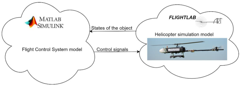
The developed automatic control system (described in Section 2.3) runs in the MATLAB/Simulink environment and is connected to the FLIGHTLAB helicopter model (Figure 4).
2.3. Electrical Energy Consumption Model
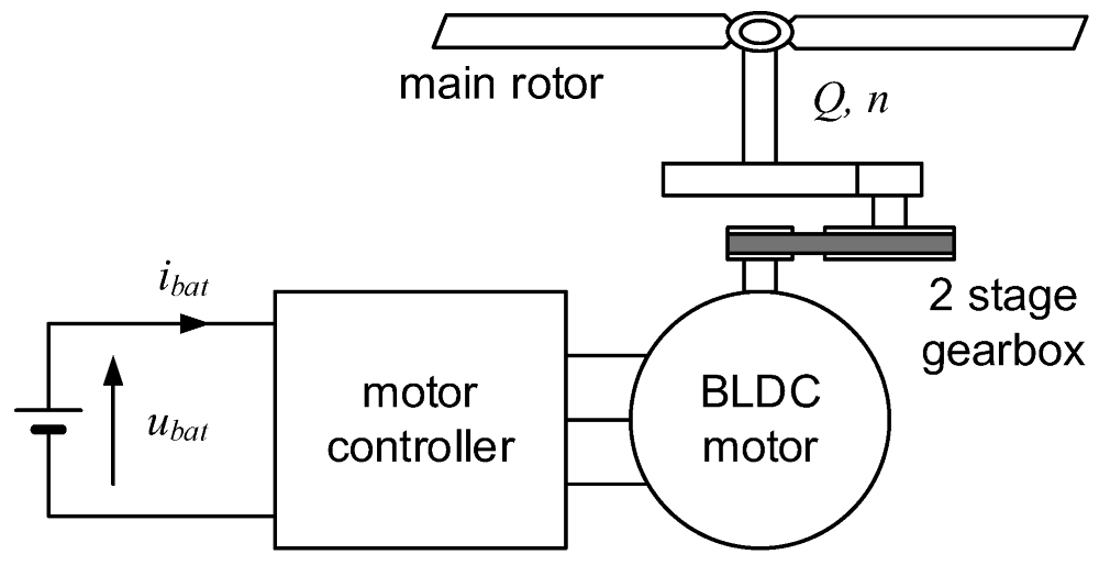
The scheme of the drive system for the helicopter is provided in Figure 5. The main rotor characteristics and operating point are the most influential factors with respect to electrical energy consumption. However, the drive train efficiency, which differs depending on the operating point of the main rotor, has a considerable influence on the helicopter’s energy consumption. Thus, when energy consumption is analyzed, apart from a consideration of the main rotor’s properties, it is also necessary to ascertain the power train efficiency map.
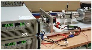
To develop the model of the consumed energy depending on the operating point of the main rotor, a stationary testbed of the whole power train system (including the gearbox, motor, motor controller, and the supply unit) was constructed, which is shown in Figure 6. The data of the power train main components are provided in Table 3. The real main rotor was replaced by an electric generator with controlled load to precisely set and measure the operating point of load, which is defined as the rotational speed and torque. Instead of a battery, a DC supply unit was used to avoid frequent charging of the battery during tests. The battery efficiency was determined separately and included in the final estimate of energy consumption.
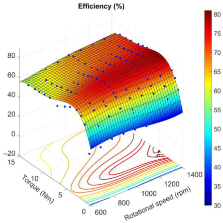
Electric power Pe was calculated as ubat ibat, whereas mechanical power Pm from the main rotor shaft was calculated as the product of torque Q and rotational speed n. Battery power losses were determined as . Battery resistance ( was estimated separately by measuring the battery terminals’ voltage drops during loading and unloading at different battery states of charge (SOC). It must be noted that major power losses were related to the powertrain; thus, a potential error in the determination of battery losses due to possible changes in battery internal resistance [54] would have a negligible influence on the efficiency map for the whole system. The total efficiency function is shown in Figure 7.
The equation of power train efficiency as a function of speed and torque was determined as:
Electrical power was calculated by Equation (2), for which the information about torque and speed from the propeller model and the efficiency as a function of torque and speed were known, whereas the consumed energy would be the result of electric power integration over the measured time period, as in Equation (3).
The scheme used for the energy consumption calculation is provided in Figure 8. The model of the main rotor returned the value of torque for given flight conditions and the reference speed was set arbitrarily to verify its influence on the flight parameters and total energy consumption during the mission.
2.4. Automatic Flight Control System
A helicopter is an underactuated vehicle that has six degrees of freedom and four independent control signals. A helicopter’s main and tail rotors produce the lift and thrust forces and provide attitude control. There are four independent control variables in a helicopter of the classical configuration: main rotor collective pitch (XC), main rotor lateral and longitudinal cyclic pitch (XA and XB), and tail rotor collective pitch (XP). The main rotor thrust is controlled by its collective pitch and is used to produce the helicopter’s lift and thrust forces. The cyclic pitch of the main rotor controls the direction of its thrust vector by tilting it in the longitudinal or lateral plane. The vertical part of the thrust vector is the lift force while the horizontal part is the propulsive force, which, when combined, enable flight forward, rearward, or sideward in the horizontal plane, depending on the control signals. The tail rotor is used to compensate for the main rotor torque and control the helicopter’s yaw. This configuration of the aircraft results in the fact that the helicopter’s (fuselage) pitch and roll are involved in acceleration and deceleration, especially when a stiff rotor is used, which is typical in the design of a small UAV helicopter.
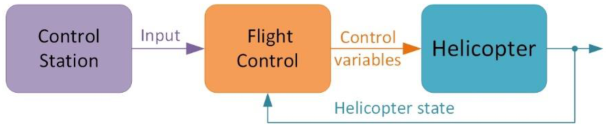
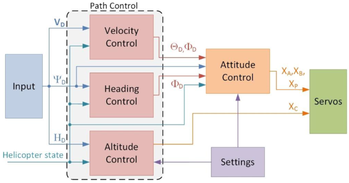
The main aspect of the flight control system for an unmanned helicopter is onboard Autopilot (Figure 9), which receives the demanded values of the controlled variables from an external Control Station. The Autopilot provides control signals to the rotors depending on the demanded and measured values of the flight parameters with respect to the helicopter’s dynamic performance and limitations. The Autopilot enables the helicopter’s path control, which is why it consists of two parts: Path Control and Attitude Control (Figure 10). The Control Station provides the demanded values of flight altitude , heading , and velocity vector , for which the latter encompasses the demanded airspeed and side velocity . The Path Control system governs the velocity, heading, and altitude control. The altitude controller calculates the main rotor’s collective pitch control signal while the velocity and heading controllers provide the demanded helicopter pitch and roll values for the Attitude Control system. This system performs calculations of the main rotor’s longitudinal and lateral cyclic pitch and the collective pitch of the tail rotor . The control vector consists of all the main and tail rotors’ control signals: .
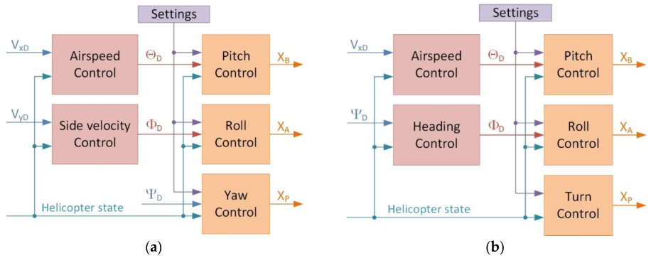
The designed automatic flight control system allows for control of the helicopter in hover and cruise flight conditions. The structure and functionality of the Path and Attitude Control segments are generally different for each flight phase (Figure 11), but only altitude control does not depend on the control mode. The hover control mode is active when the helicopter’s airspeed is less than 4.5 ft/s. When this value is exceeded, the cruise control mode is automatically engaged. The main task of the hover mode is to maintain the equilibrium state, control the heading and altitude, and execute small (with velocity less than 4.5 ft/s) horizontal movements. Therefore, the Path Control segment consists of airspeed (forward velocity) and side velocity controllers; these controllers calculate the demanded pitch and bank angle, respectively, with respect to the demanded values of airspeed and side velocity. The helicopter’s heading is directly controlled by the yaw controller of the Attitude Control. The main task of the cruise mode is to control the velocity (above 4.5 ft/s), heading and altitude, and perform banked turns (coordinated turns). In this mode, the demanded pitch angle is calculated by the airspeed controller, as in the hover mode, and the demanded bank angle is provided by the heading controller. The turn controller compensates for the helicopter’s sideslip, so the Heading, Bank, and Turn Control subsystems together are used to make a coordinated turn. Since the main rotor is used to both generate lift and control the helicopter, additional flight parameters need to be controlled. This allows for smooth and effective control of the helicopter, taking into account its dynamic properties and design constraints. Therefore, additional settings are applied to the controllers of the Attitude Control segment. From the point of view of the presented research, the most important settings are as follows: pitch angle, bank angle, and vertical speed limits. All these limitations enable smooth control of the helicopter and reduce the risk of exceeding the main rotor limitations during maneuvers such as acceleration, climbing, and turning. The pitch angle and climb rate limits are used to enhance the longitudinal control of the helicopter. Pitch angle and vertical speed limitations are used to improve the longitudinal control of the helicopter. The pitch angle limit enables indirect control of longitudinal acceleration, while the vertical speed limit reduces the maximum climb rate. The descent rate limiter is fixed and set to a value that avoids the vortex ring state of the main rotor. The bank angle limit is used to control the turn rate of the helicopter. The controllers used in the Path and Attitude Control segments were designed using the classical control theory. Additional cross couplings between the control and state variables were applied to enable the proper flight performance of the helicopter. The control laws were optimized for one set of autopilot settings and the main rotor RPM settings, whose change may cause a difference in the system performance. Therefore, the demanded values of pitch, roll, and rate of climb cannot be taken literally, but as intermediate values between the limit values that can be obtained under a given configuration of the autopilot and RPM.
3. Energy Consumption Analysis
3.1. Methodology
The computer simulation tests were performed to execute helicopter energy consumption analysis during particular maneuvers and flight conditions and for different main rotor RPM values. The aim of these tests was to analyze how the main rotor RPM influences the helicopter’s electric energy expenditure and flying qualities. Five values of the main rotor RPM were chosen for all tests: 800, 900, 1000, 1100, and 1200. Five typical maneuvers and flight conditions were chosen for these tests: hover, cruise flight, acceleration from hover to cruise flight, climb, and turn. The tests were performed for various RPM values of the main rotor and demanded control variables and autopilot settings. The tests covered acceleration to various cruise speeds, climbing to various altitudes, and turning to various azimuths. Various autopilot settings were also included in the tests. Various demanded pitch and bank angles as well climb rates were tested. The acceleration and the turn rates are not directly controlled by the autopilot. Therefore, an indirect method was used during the tests. The helicopter’s pitch and bank angles are used to control the helicopter’s motion; the maximum values of both angles limit the values of acceleration and the turn rate, respectively. Therefore, during the tests, they were used to indirectly limit the maximum values of these flight parameters. This approach makes it possible to study the effect of RPM not only on the dynamic characteristics of the helicopter but also on the quality of autopilot performance. For the same reason, simulation tests without turbulence were performed. The flight disturbances caused by the turbulence could affect the assessment of the effect of RPM on the control performance of the helicopter. All simulation tests were performed for a helicopter mass of 7.23 kg.
The simulation testbed, which was presented in Section 2, was developed using the FLIGHTLAB and MATLAB/Simulink simulation software systems. Both were run on the same computer with a Linux operating system and exchanged data while the simulation was running. Due to the cooperation of the two simulation environments, the simulation model was sensitive to initial conditions, and some flight disturbances appeared at the beginning of the simulation. Therefore, each simulation began with a 50 s hover during which the helicopter was stabilized and autopilot parameters were updated. The simulation tests were divided into five parts: hover, cruise, acceleration, climbing, and turn tests. The test procedure was the same in each case. The simulation models were first prepared for the simulation of the selected flight conditions. The dynamic models were trimmed at the demanded velocity, altitude, heading, and weight. The AFCS parameters were also set. Next, the simulations were run for a demanded time period. A simulation was run multiple times for each test case separately and the results were recorded. Finally, the simulation data were processed and analyzed to determine the energy consumption in each phase of flight. It was assumed that a particular maneuver was completed when the control error value (the difference between the values of the demanded and controlled variables) fell below the limit value. The conclusions regarding energy consumption were formulated based on the results of these analyses.
3.2. Hover Tests
The tests were performed at a constant altitude. During each test, the helicopter’s flight and energy parameters were obtained. The test was repeated for all the chosen values of the main rotor RPM. The tests plan is shown in Table 4.
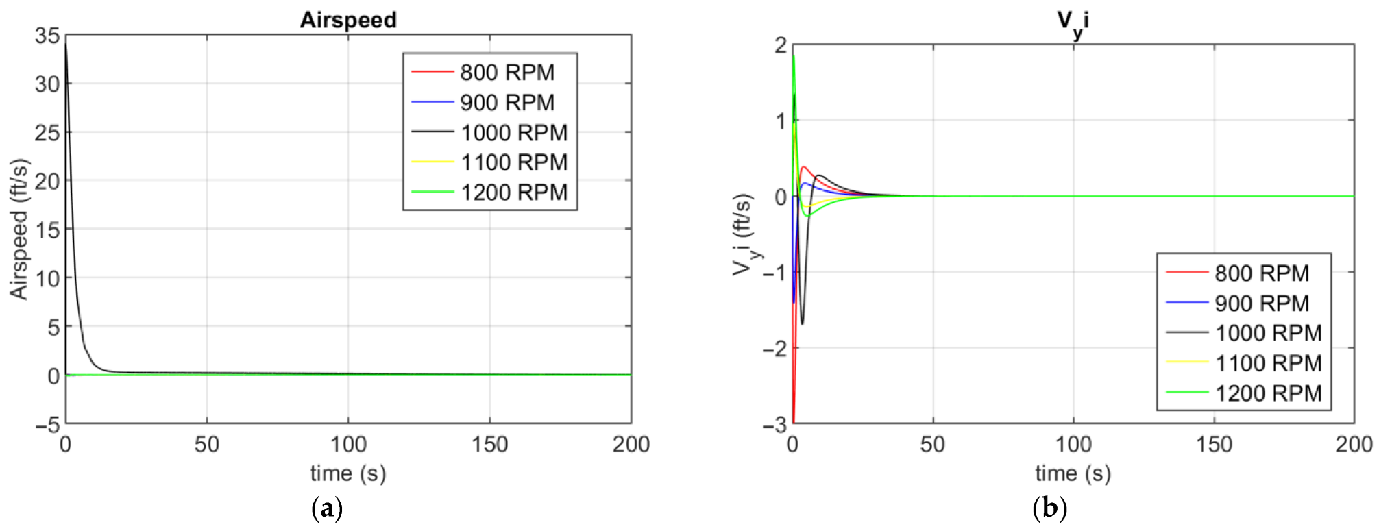
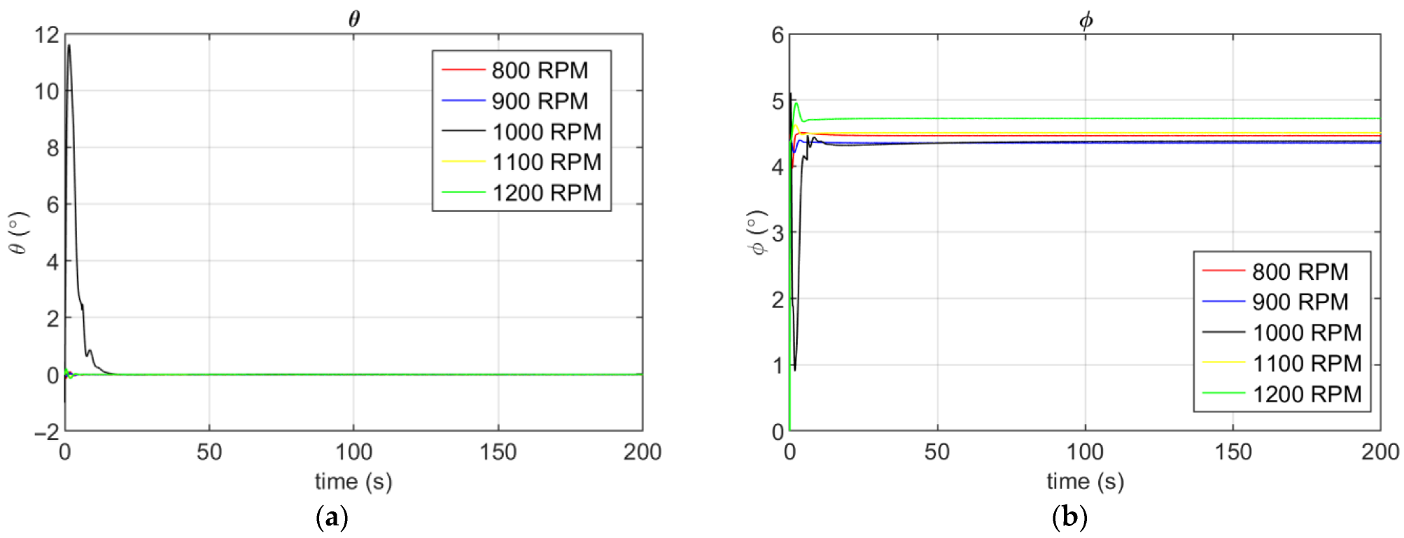
Examples of the hover test results are shown in Figure 12, Figure 13 and Figure 14. These charts present the airspeed, side velocity, altitude, pitch and bank angles, and energy usage while hovering at the altitude of 33.81 ft. The helicopter maintained a hover, and the airspeed, side velocity, and altitude remained constant. The helicopter needed about 50 s to stabilize the flight after starting the simulation, as was mentioned above. Therefore, this part of the simulation was not subjected to energy analysis. The different bank angles can be observed for various RPM values. Different RPM values resulted in different rotor operating conditions and thus different values of torque, which had to be compensated by the tail rotor thrust. In turn, the lateral force from the tail rotor had to be compensated by changing the bank angle. It can be noted that the smallest roll angle occurs at 1000 RPM, which suggests that, for this value, the torque for hovering is the smallest. However, as the results show, this fact does not affect energy consumption. Total energy consumption increases as RPM increases. Energy consumption during the last 50 s of the simulation is shown in the Table 5.
3.3. Cruise Flight Tests
The tests were performed at a constant altitude and heading and at various speeds. The nominal cruise velocity of 34 ft/s was chosen as the reference value for these tests. In addition, 1/3 and 2/3 of this value were selected. The tests were repeated for all the chosen values of the main rotor RPM. The tests’ plan is shown in Table 6.
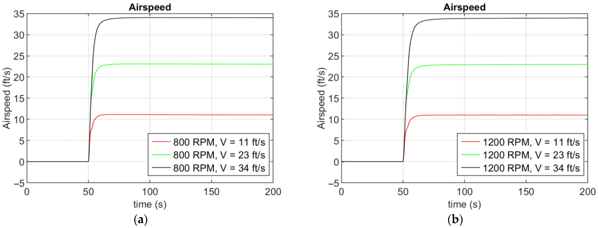
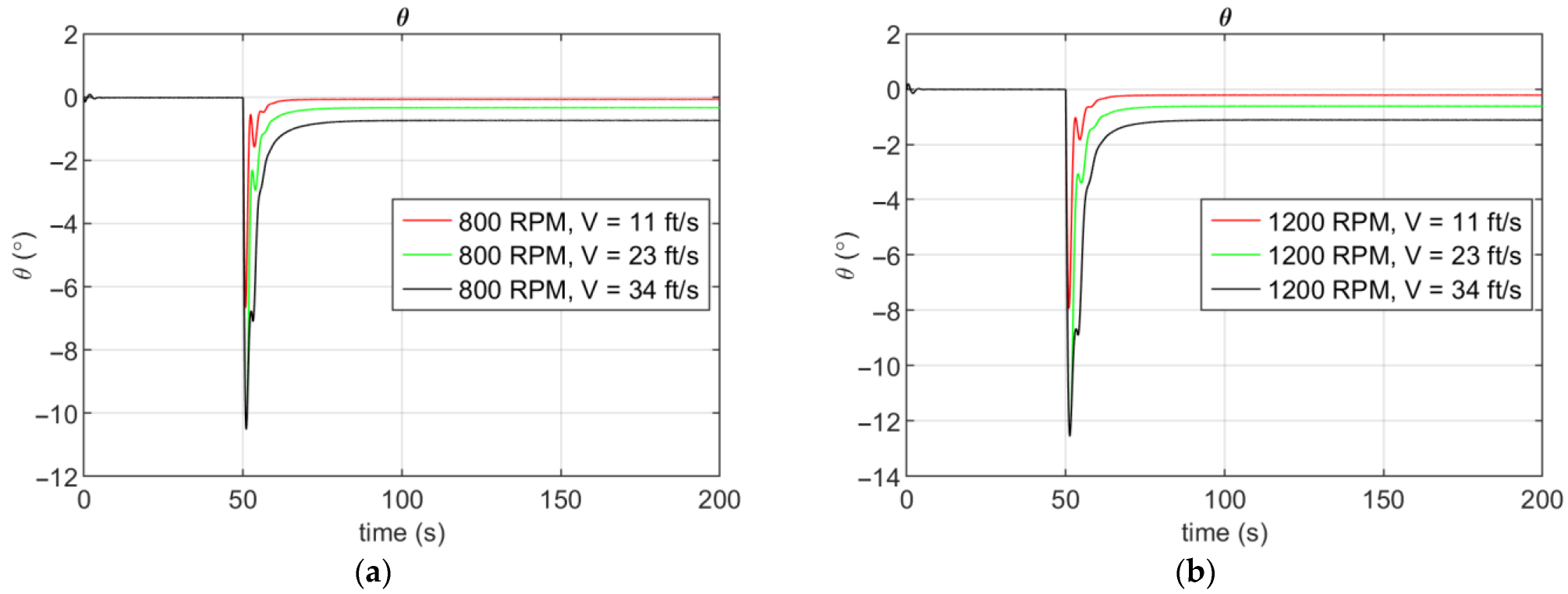
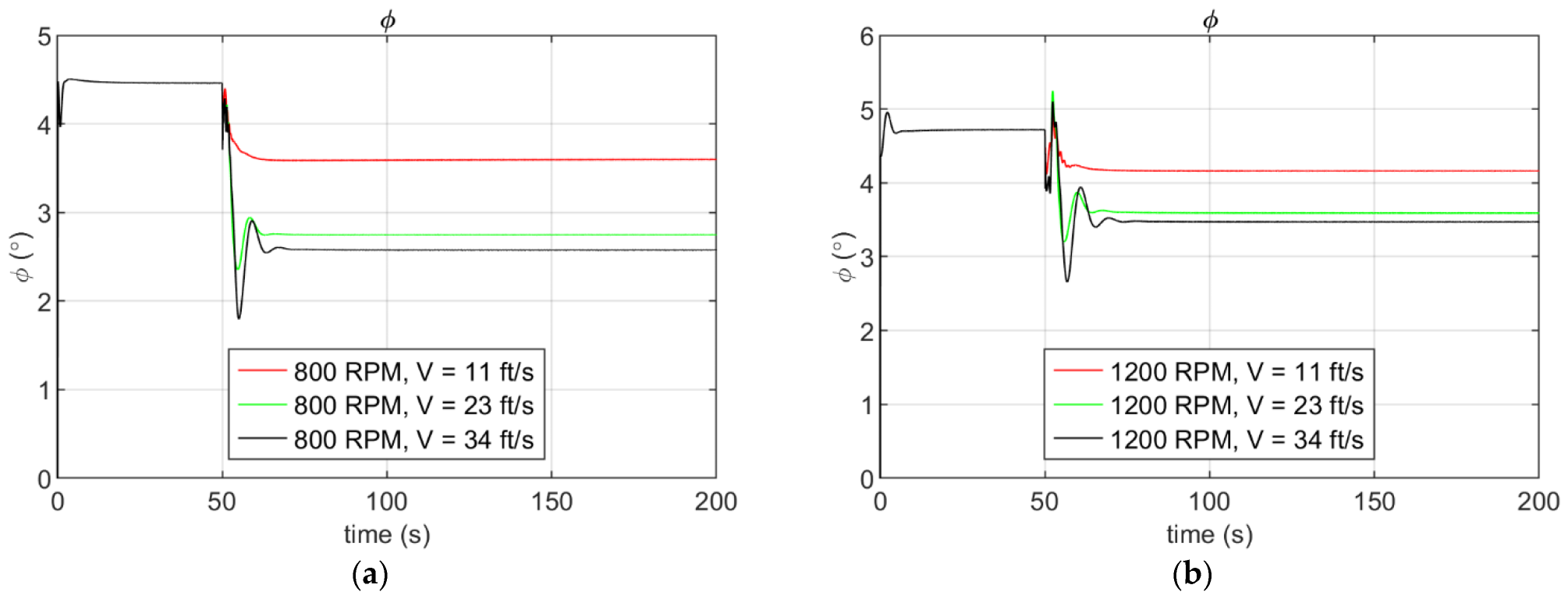
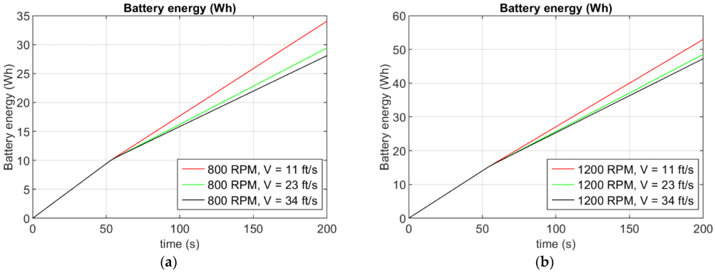
Figure 15, Figure 16, Figure 17 and Figure 18 show examples of the tests of cruise flight. The charts present the airspeed, pitch and bank angles, and energy usage during cruise flight at the altitude of 33.81 ft and different demanded airspeeds. For comparison, the figures also show the results for 800 and 1200 RPM. The helicopter maintained a hover for the first 50 s of flight; then, for the next 50 s, it accelerated to the demanded velocity and, finally, flew at a steady speed until 200 s. As it can be seen, a higher value of speed required a higher pitch angle and a smaller bank angle. This changed the operating conditions of the main and tail rotors and thus changed the level of energy consumption. The energy consumption during the last 50 s of the simulation is shown in Table 7. This shows that an increase in RPM results in an increase in energy consumption, and for about 60–80% of cases it depends on the speed. Moreover, energy consumption decreases with the increasing speed (about 15–25% depends on RPM), which is due to the fact that the airspeed of 34 ft/s is the cruising airspeed for this helicopter design.
3.4. Accelaration Tests
The acceleration tests were conducted to analyze the helicopter’s flight and energy performance while accelerating from hover to cruise velocity. The tests were performed according to a constant altitude and selected values of the demanded cruise velocity. The acceleration of the helicopter depends on the value of the module of the horizontal component of the thrust vector of the main rotor, i.e., the pitch angle. Therefore, acceleration tests were conducted for different values of this angle. This made it possible to determine the optimal control strategy of the helicopter during acceleration. The tests’ plan is shown in Table 8. All the flights were performed at a constant altitude (33.81 ft) and heading (0 deg).
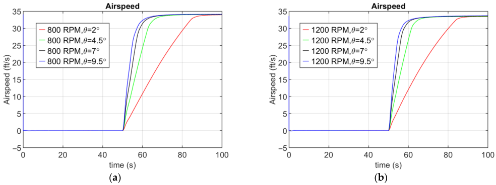
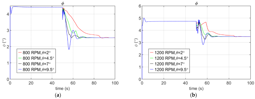
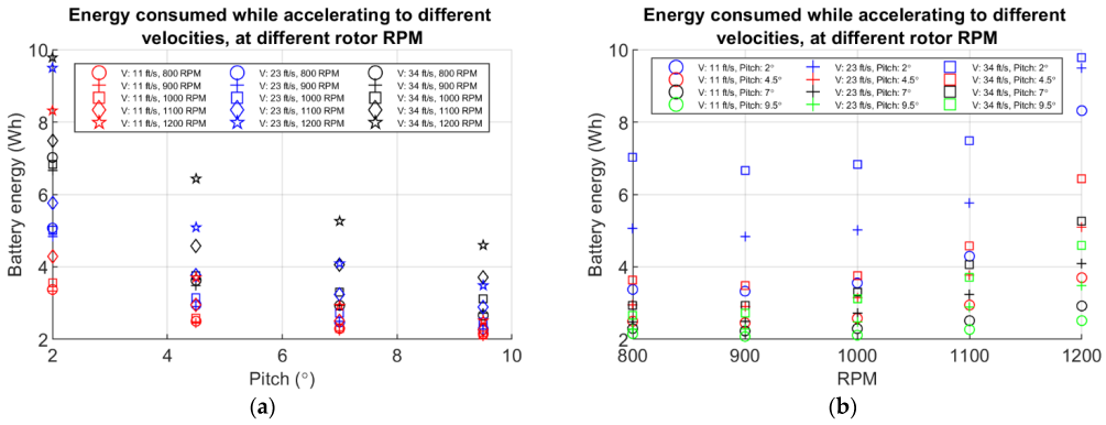
Examples of the test results are shown in Figure 19, Figure 20, Figure 21 and Figure 22. These charts present the airspeed, pitch and bank angles, and energy usage during acceleration from a hover to the speed of 34 ft/s for different demanded pitch angles. For comparison, the figures show the results for 800 and 1200 RPM. The helicopter maintained a hover for the first 50 s of flight; then, for the next 50 s, it accelerated to the demanded velocity. A lower pitch angle resulted in a longer acceleration time and thus higher energy consumption. Moreover, for the higher pitch, the differences in energy consumption were smaller, which was due to the fact that the acceleration time was so short that even a constant value of the pitch angle was not established. The levels of energy consumption during particular maneuvers and during the last 50 s of flight—including the acceleration maneuver and the flight at constant speed—for RPM values of 800 and 1200 are presented in Table 9 and Figure 23. The results show that accelerating with a higher pitch angle reduces energy consumption, which is mainly due to the fact that such a maneuver takes less time. Analyzing the last 50 s of flight, it can be seen that, from the perspective of the flight duration, energy consumption during acceleration has a small impact on the total energy used during the entire flight. It can also be noted that lower energy consumption occurred at 900 RPM.
3.5. Climbing Rate Tests
Climbing rate tests were conducted to analyze the helicopter’s flight and energy performance during a climb from 33.81 ft to selected altitudes during cruise flight with a constant speed of 34 ft/s. The thrust of the main rotor is one of the factors that has a significant impact on energy consumption. During climbing flight, thrust must be increased to achieve the demanded vertical speed. Therefore, it is necessary to study how a helicopter’s vertical speed affects the increase in energy consumption. The results of this research will enable the selection of the optimal (from an energy consumption perspective) climbing trajectory. The tests’ plan is shown in Table 10.
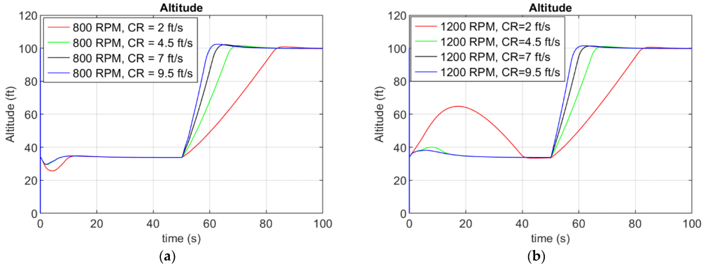
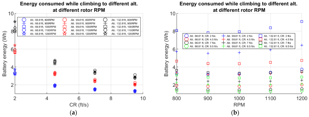
Figure 24, Figure 25, Figure 26, Figure 27 and Figure 28 and Table 11 show the climbing rate test results. The altitude, vertical speed, pitch angle, and energy usage during acceleration to the speed of 34 ft/s and climbing to the 99.81 ft for different vertical speeds are presented. For comparison, the figures show the results for 800 and 1200 RPM. The helicopter accelerated to the cruise speed for the first 50 s of flight; then, for the next 50 s, it climbed to the demanded altitude. A higher vertical velocity required less energy. As in the case of acceleration, this resulted from the fact that the maneuver with a higher climb rate took less time. However, over a longer time interval (50 s, in this case), the level of energy expended was similar. This is due to the fact that, regardless of the rate of climb, the parasite drag had a similar value. The slight differences are due to the fact that the ascent at a low climbing rate is smooth and does not cause much disturbance of the helicopter attitude. Therefore, energy consumption during the climbing maneuver itself is different, but from the perspective of flight over a long term, the difference is small. Moreover, lower energy consumption occurred at 1000 RPM in most cases. It should be noted that some problems with altitude stabilization during the acceleration phase occurred at a low vertical velocity at 1200 RPM. There were also differences in the attained values of vertical velocity. This is due to the fact that the main rotor is used both to generate lift and control the helicopter, and its dynamic characteristics strongly depend on the RPM. In addition, the control system is designed for a single RPM value. This shows the limitations of the autopilot for these system settings.
3.6. Turn Rate Tests
Turn rate tests were conducted to analyze the helicopter’s flight and energy performance during a banked turn for various headings. The tests were performed at a constant altitude of 33.81 ft and a constant speed of 34 ft/s. The rate of the turn depends on the helicopter’s bank angle. Therefore, these tests were conducted for different values of this angle. The results of these tests can be used to plan the optimal trajectory of a helicopter. The tests’ plan is shown in Table 12.
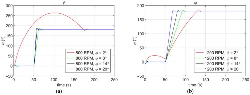
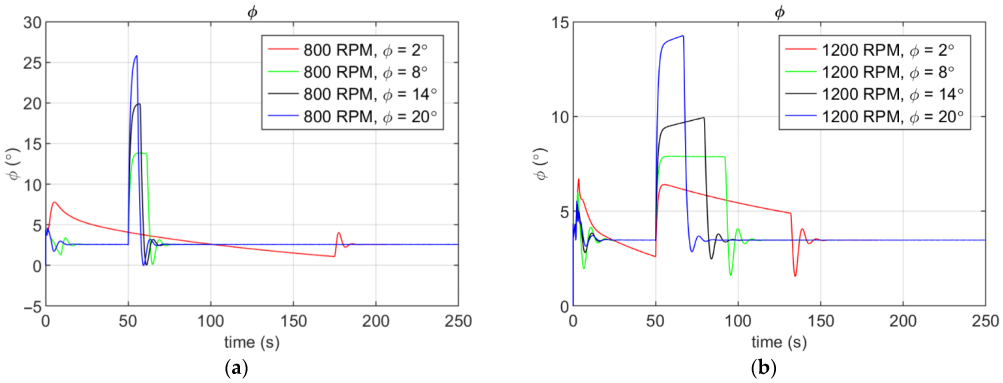
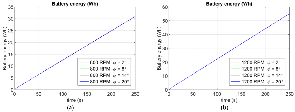
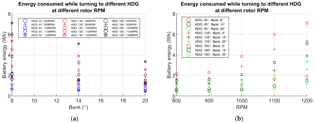
The results of the turn rate tests for 800 and 1200 RPM are shown in Figure 29, Figure 30, Figure 31 and Figure 32 as examples. The graphs show the heading, bank and pitch angles, and energy usage during acceleration to the speed of 34 ft/s and turning to 180 deg for different demanded bank angles. The helicopter accelerated to cruise speed for the first 50 s of flight; then, for the next 200 s, it performed a banked turn to the demanded heading. Figure 33 and Table 13 show the energy consumption levels acquired in the turn rate tests. As in the case of climbing, performing a turn with a higher bank angle required less energy, which was due to the fact that the maneuver takes less time. However, over a longer time interval (the last 200 s), the level of expended energy was similar, and the slight differences observed were due to the smoothness of the maneuver. Moreover, lower RPM required lower energy to perform this maneuver. It can also be seen that some problems with the heading control occurred for a low bank angle at 1200 RPM, but for 800 RPM, the helicopter was out of control. This indicates serious limitations of the autopilot with respect to these system settings and RPM values. In addition, differences can be observed in the achieved values of the bank angle, which, as in the case of the climb test, were due to the dynamic properties of the main rotor. The main rotor is used to control both pitch and roll. However, due to the limited level of energy generated, priority was given to pitch control. Moreover, the helicopter’s roll was also used to compensate for the lateral force generated by the tail rotor. Therefore, the real value of the roll angle depended on both the demanded value and the autopilot and RPM settings.
4. Conclusions
An energy consumption analysis of a UAV helicopter is presented in this paper. The dedicated simulation testbed developed in the combined FLIGHTLAB/MATLAB/Simulink environment was used to simulate and analyze energy consumption for different flight conditions and system settings. The model of the ARCHER helicopter was built using the FLIGHTLAB software and validated using the flight test data. The automatic flight control system was designed using MATLAB/Simulink software and allowed for the simulation of the helicopter’s autonomous flight in all flight conditions and maneuvers. The advanced model of energy consumption that includes the electric motor, gear, and main rotor characteristics was designed, validated using a laboratory test bed, and used in this research.
The objective of the simulation tests was to investigate the effect of the main rotor RPM and automatic flight control system settings on the energy consumption while accounting for the degradation of the control qualities. The results showed that a helicopter’s energy consumption strongly depends on the main rotor RPM and the flight speed. Lower energy was used when the helicopter flew around the cruise velocity of 34 ft/s. A lower RPM resulted in lower energy consumption but also reduced the helicopter’s controllability in some maneuvers and AFCS settings. The results suggest the possibility of adjusting the main rotor RPM to actual flight conditions in order to reduce energy consumption throughout a flight. However, it is necessary to use an adaptive control system to take full advantage of RPM variability. The time domain analysis of the simulation results indicated its good capability for estimating helicopter energy consumption and usefulness for mission plan optimization. The scientific significance of this work is that the research results can be used for the development of small, unmanned helicopters of a classic configuration. A detailed analysis of the economic and ecological potential of these types of aircraft will allow for their wider commercial use in areas where other types of rotorcraft are less effective or cannot be used. It is envisaged that such research would be useful for detailed mission planning (considering each particular maneuver) and the optimization of new helicopters and automatic flight control system designs. The presented complex energy consumption model and large set of simulation data added in the Supplementary Materials, which are not found in the earlier literature, will be helpful for the development of new UAV helicopter designs in accordance with the green aircraft concept.
Further research may concentrate on simulation tests under various environmental conditions to estimate the practical range of RPM variation with wind and turbulence. Moreover, the simulation test bed could be expanded to include the ability to test real autopilots using the HIL method, which would enable optimal autopilot alignment with a given helicopter.
Supplementary Materials
The following supporting information can be downloaded at: https://www.meil.pw.edu.pl/daas/DAAS2/Research/Projects/HELINERGY (accessed on 19 January 2023), simulation data that were used to produce Figure 12, Figure 13, Figure 14, Figure 15, Figure 16, Figure 17, Figure 18, Figure 19, Figure 20, Figure 21, Figure 22, Figure 23, Figure 24, Figure 25, Figure 26, Figure 27, Figure 28, Figure 29, Figure 30, Figure 31, Figure 32 and Figure 33 and more.
Author Contributions
Conceptualization, M.Ż., G.I., P.B. and S.T.; methodology, M.Ż., G.I. and P.B.; software, P.B. and P.F.; validation, P.B., G.I., P.F., M.E. and M.Ż.; formal analysis, G.I. and M.Ż.; investigation, G.I., P.F. and M.E.; resources, S.T.; data curation, M.E.; writing—original draft preparation, S.T., G.I. and M.Ż.; writing—review and editing, S.T. and M.Ż; visualization, M.E., P.F. and M.Ż.; supervision, M.Ż.; project administration, S.T.; funding acquisition, S.T. All authors have read and agreed to the published version of the manuscript.
Funding
This research was funded by POB Energy of Warsaw University of Technology within the Excellence Initiative: Research University (IDUB) Programme, the grant No. 1820/37/Z01/POB7/2021.
Data Availability Statement
Simulation data are available as Supplementary Materials. Simulation information will be available on request to the corresponding author’s email with appropriate justification.
Conflicts of Interest
The authors declare no conflict of interest. The funders had no role in the design of the study; in the collection, analyses, or interpretation of data; in the writing of the manuscript, or in the decision to publish the results.
Nomenclature
The following abbreviations and symbols are used in this manuscript:
| Latin symbols | |
| energy, (J) | |
| Demanded altitude, (ft) | |
| battery current, (A) | |
| rotational speed (RPM) | |
| electric power, (W) | |
| mechanical power, (W) | |
| torque (Nm) | |
| battery resistance, () | |
| battery voltage, (V) | |
| components of linear velocity in reference frame, (m/s) | |
| Demanded forward and side velocity, (ft/s) | |
| Demanded helicopter velocity, (ft/s) | |
| main rotor lateral and longitudinal cyclic pitch, and main rotor collective pitch | |
| tail rotor collective pitch | |
| Greek symbols | |
| total efficiency function | |
| helicopter attitude angles, (deg) | |
| demanded attitude angles for inner loop of AFCS, (deg) | |
| Abbreviations | |
| AFCS | Automatic Flight and Control System |
| BLDC | Brushless Direct Current |
| E-VTOL | Electric Vertical Take-off and Landing |
| Battery State of Charge, (%) | |
| UAV | Unmanned Aerial Vehicle |
References
- Magnussen, Ø.; Ottestad, M.; Hovland, G. Multicopter design optimization and validation. Model. Identif. Control. 2015, 36, 67–79. [Google Scholar] [CrossRef] [Green Version]
- Wu, J.; Wang, H.; Huang, Y.; Su, Z.; Zhang, M. Energy management strategy for solar-powered UAV long-endurance target tracking. IEEE Trans. Aerosp. Electron. Syst. 2019, 55, 1878–1891. [Google Scholar] [CrossRef]
- Dwivedi, V.S.; Salahudden, S.; Giri, D.K.; Ghosh, A.K.; Kamath, G.M. Optimal energy utilization for a solar-powered aircraft using sliding-mode-based attitude control. IEEE Trans. Aerosp. Electron. Syst. 2021, 57, 105–118. [Google Scholar] [CrossRef]
- Lee, D.S.; Periaux, J.; Gonzalez, L.; Srinivas, K. Robust multi-objective and multidisciplinary design optimization of UAV using advanced evolutionary algorithms. In Proceedings of the 47th AIAA Aerospace Sciences Meeting including the New Horizons Forum and Aerospace Exposition, Orlando, FL, USA, 5–8 January 2009. [Google Scholar]
- Zheng, X.; He, S.; Lin, D. Constrained trajectory optimization with flexible final time for autonomous vehicles. IEEE Trans. Aerosp. Electron. Syst. 2021, 58, 1818–1829. [Google Scholar] [CrossRef]
- Bibik, P.; Narkiewicz, J.; Zasuwa, M.; Żugaj, M. Modeling of quadrotor dynamics for research and training simulator. In Proceedings of the 39th European Rotorcraft Forum, Moscow, Russia, 3–6 September 2013. [Google Scholar]
- Jacewicz, M.; Żugaj, M.; Głębocki, R.; Bibik, P. Quadrotor model for energy consumption analysis. Energies 2022, 15, 7136. [Google Scholar] [CrossRef]
- Zhang, J.; Campbell, J.F.; Sweeney, D.C.; Hupman, A.C. Energy consumption models for delivery drones: A comparison and assessment. Transp. Res. Part D Transp. Environ. 2021, 90, 102668. [Google Scholar] [CrossRef]
- Wu, M.; Chen, W.; Tian, X. Optimal energy consumption path planning for quadrotor UAV transmission tower inspection based on simulated annealing algorithm. Energies 2022, 15, 8036. [Google Scholar] [CrossRef]
- Zeng, Y.; Xu, J.; Zhang, R. Energy minimization for wireless communication with rotary-wing UAV. IEEE Trans. Wirel. Commun. 2019, 18, 2329–2345. [Google Scholar] [CrossRef] [Green Version]
- Beigi, P.; Rajabi, M.S.; Aghakhani, S. An overview of drone energy consumption factors and models. arXiv 2022, arXiv:2206.10775. [Google Scholar] [CrossRef]
- Jia, G.; Li, C.; Li, M. Energy-Efficient Trajectory Planning for Smart Sensing in IoT Networks Using Quadrotor UAVs. Sensors 2022, 22, 8729. [Google Scholar] [CrossRef]
- Morbidi, F.; Cano, R.; Lara, D.; Morbidi, F.; Cano, R.; Lara, D.; Generation, M.P.; Morbidi, F.; Cano, R.; Lara, D. Minimum-Energy Path Generation for a Quadrotor UAV. In Proceedings of the International Conference on Robotics and Automation, Stockholm, Sweden, 16–21 May 2016; pp. 2–8. [Google Scholar]
- Lu, P.; Liu, M.; Zhang, X.; Zhu, G.; Li, Z.; Su, C.-Y. Neural network based adaptive event-triggered control for quadrotor unmanned aircraft robotics. Machines 2022, 10, 617. [Google Scholar] [CrossRef]
- Xiao, S.; Tan, X.; Wang, J. A Simulated annealing algorithm and grid map-based UAV coverage path planning method for 3D reconstruction. Electronics 2021, 10, 853. [Google Scholar] [CrossRef]
- Wu, F.; Yang, D.; Xiao, L.; Cuthbert, L. Energy consumption and completion time tradeoff in rotary-wing UAV enabled WPCN. IEEE Access 2019, 7, 79617–79635. [Google Scholar] [CrossRef]
- Fouad, Y.; Rizoug, N.; Bouhali, O.; Hamerlain, M. Optimization of energy consumption for quadrotor UAV. In Proceedings of the International Micro Air Vehicle Conference and Flight Competition (IMAV) 2017, Toulouse, France, 18–21 September 2017; pp. 215–222. [Google Scholar]
- Steup, C.; Parlow, S.; Mai, S.; Mostaghim, S. Generic component-based mission-centric energy model for micro-scale unmanned aerial vehicles. Drones 2020, 4, 63. [Google Scholar] [CrossRef]
- Chang, C.-W.; Chen, S.; Wen, C.-Y.; Li, B. An actuator allocation method for a variable-pitch propeller system of quadrotor-based UAVs. Sensors 2020, 20, 5651. [Google Scholar] [CrossRef]
- Wang, Y.; Wang, Y.; Ren, B. Energy saving quadrotor control for field inspections. IEEE Trans. Syst. Man Cybern. Syst. 2022, 52, 1768–1777. [Google Scholar] [CrossRef]
- Chovancová, A.; Fico, T.; Duchoň, F.; Dekan, M.; Chovanec, Ľ.; Dekanová, M. Control methods comparison for the real quadrotor on an innovative test stand. Appl. Sci. 2020, 10, 2064. [Google Scholar] [CrossRef] [Green Version]
- Aguilar-Lopez, J.M.; Garcia, R.A.; Bordons, C.; Camacho, E.F. Development of the energy consumption model of a quadrotor using voltage data from experimental flights. In Proceedings of the 2022 IEEE 17th International Conference on Control & Automation (ICCA), Naples, Italy, 27–30 June 2022; pp. 432–437. [Google Scholar] [CrossRef]
- Alyassi, R.; Khonji, M.; Karapetyan, A.; Chau, S.C.-K.; Elbassioni, K.; Tseng, C.-M. Autonomous recharging and flight mission planning for battery-operated autonomous drones. IEEE Trans. Autom. Sci. Eng. 2022, 1–13. [Google Scholar] [CrossRef]
- Zhou, C.; Xu, A.; Wang, F.; Chen, M.; Li, W.; Yin, R. Performance optimization of helicopter rotor in hover based on CFD simulation. Math. Probl. Eng. 2022, 2022, 3146658. [Google Scholar] [CrossRef]
- Kocjan, J.; Kachel, S.; Rogólski, R. Helicopter main rotor blade parametric design for a preliminary aerodynamic analysis supported by CFD or panel method. Materials 2022, 15, 4275. [Google Scholar] [CrossRef]
- Xie, J.; Xie, Z.; Zhou, M.; Qiu, J. Multidisciplinary aerodynamic design of a rotor blade for an optimum rotor speed helicopter. Appl. Sci. 2017, 7, 639. [Google Scholar] [CrossRef] [Green Version]
- Xu, A.; Chen, M.; Wang, F.; Li, L. Research on dynamic model of the small-scale compound coaxial unmanned helicopter. In Proceedings of the 2022 International Conference on Electrical, Control and Information Technology, Kunming, China, 25–27 March 2022. [Google Scholar]
- Yeo, H. Design and aeromechanics investigation of compound helicopters. Aerosp. Sci. Technol. 2019, 88, 158–173. [Google Scholar] [CrossRef]
- Graham, B.D.; Hyeonsoo, Y. Performance and loads study of a high-speed compound helicopter. J. Am. Helicopter Soc. 2018, 63, 1–15. [Google Scholar]
- Cao, Y.; Wang, Y.; Song, H.; Li, Q.; Zhang, H. The unidirectional auxiliary surface sliding mode control for compound high-speed helicopter. In Proceedings of the IEEE CSAA Guidance, Navigation and Control Conference, Xiamen, China, 10–12 August 2018. [Google Scholar]
- Citroni, R.; Di Paolo, F.; Livreri, P. A novel energy harvester for powering small UAVs: Performance analysis, model validation and flight results. Sensors 2019, 19, 1771. [Google Scholar] [CrossRef] [Green Version]
- Liu, Q.; Zhang, Z.; Jia, T.; Wang, L.; Zhao, D. Energy consumption analysis of helicopter traction device: A modeling method considering both dynamic and energy consumption characteristics of mechanical systems. Energies 2022, 15, 7772. [Google Scholar] [CrossRef]
- Trigona, C.; Andò, B.; Baglio, S. Measurements and investigations of helicopter-induced vibrations for kinetic energy harvesters. In Proceedings of the IEEE Sensors Applications Symposium, Sophia Antipolis, France, 11–13 March 2019. [Google Scholar]
- Ma, K.; Chen, L.; Luo, K. Study on energy management system of helicopter. In Proceedings of the CSAA/IET International Conference on Aircraft Utility Systems, Online, 18–21 September 2020. [Google Scholar]
- Cole, J.A.; Rajauski, L.; Loughran, A.; Karpowicz, A.; Salinger, S. Configuration study of electric helicopters for urban air mobility. Aerospace 2021, 8, 54. [Google Scholar] [CrossRef]
- Donateo, T.; Carla, A.; Avanzini, G. Fuel consumption of rotorcrafts and potentiality for hybrid electric power systems. Energy Convers. Manag. 2018, 164, 429–442. [Google Scholar] [CrossRef]
- Cutler, M.; Kemal Ure, N.; Michini, B.; How, J.P. Comparison of fixed and variable pitch actuators for agile quadrotors. In AIAA Guidance; Navigation, and Control Conference (GNC): Portland, OR, USA, 2011. [Google Scholar]
- Xie, J.; Guan, N.; Zhou, M.; Xie, Z. Study on the mechanism of the variable-speed rotor affecting rotor aerodynamic performance. Appl. Sci. 2018, 8, 1030. [Google Scholar] [CrossRef]
- Padfield, G. Helicopter Flight Dynamics: The Theory and Application of Flying Qualities and Simulation Modelling, 2nd ed.; Blackwell Publishing Ltd.: Oxford, UK, 2007. [Google Scholar]
- Manimala, B.J.; Walker, D.J.; Padfield, G.D.; Voskuijl, M.; Gubbels, A.W. Rotorcraft simulation modelling and validation for control law design. Aeronaut. J. 2007, 111, 77–88. [Google Scholar] [CrossRef]
- Xie, Y.; Savvaris, A.; Tsourdos, A. Fuzzy logic based equivalent consumption optimization of a hybrid electric propulsion system for unmanned aerial vehicles. Aerosp. Sci. Technol. 2019, 85, 13–23. [Google Scholar] [CrossRef] [Green Version]
- Goulos, I.; Pachidis, V.; d’Ippolito, R.; Stevens, J.; Smith, C. An integrated approach for the multidisciplinary design of optimum rotorcraft operations. J. Eng. Gas Turbines Power 2012, 134, 091701. [Google Scholar] [CrossRef]
- Zhang, B.; Song, Z.; Liu, S.; Huang, R.; Liu, C. Overview of integrated electric motor drives: Opportunities and challenges. Energies 2022, 15, 8299. [Google Scholar] [CrossRef]
- Arellano-Quintana, V.M.; Merchán-Cruz, E.A.; Franchi, A. A novel experimental model and a drag-optimal allocation method for variable-pitch propellers in multirotors. IEEE Access 2018, 6, 68155–68168. [Google Scholar] [CrossRef]
- Gebauer, J.; Wagnerova, R.; Smutny, P.; Podesva, P. Controller design for variable pitch propeller propulsion drive. IFAC-PapersOnLine 2019, 52, 186–191. [Google Scholar] [CrossRef]
- Podsedkowski, M.; Konopinski, R.; Obidowski, D.; Koter, K. Variable pitch propeller for UAV-experimental tests. Energies 2020, 13, 5264. [Google Scholar] [CrossRef]
- Henderson, T.; Papanikolopoulos, N. Power-minimizing control of a variable-pitch propulsion system for versatile unmanned aerial vehicles. In Proceedings of the 2019 International Conference Robotics and Automation—ICRA, Montreal, QC, Canada, 20–24 May 2019; pp. 4148–4153. [Google Scholar]
- Chi, C.; Yan, X.; Chen, R.; Li, P. Analysis of low-speed height-velocity diagram of a variable-speed-rotor helicopter in one-engine-failure. Aerosp. Sci. Technol. 2019, 91, 310–320. [Google Scholar] [CrossRef]
- Han, D.; Pastrikakis, V.; Barakos, G.N. Helicopter performance improvement by variable rotor speed and variable blade twist. Aerosp. Sci. Technol. 2016, 54, 164–173. [Google Scholar] [CrossRef] [Green Version]
- Mistry, M.; Gandhi, F. Helicopter performance improvement with variable rotor radius and rpm. J. Am. Helicopter Soc. 2014, 59, 17–35. [Google Scholar] [CrossRef]
- Rahul, R.; Abhishek, A. Performance optimization of a variable speed and variable geometry rotor concept. J. Aircr. 2017, 54, 476–489. [Google Scholar]
- Miste, G.; Benini, E.; Garavello, A.; Alcoy, M.G. A methodology for determining the optimal rotational speed of a variable rpm main rotor/turboshaft engine system. J. Am. Helicopter Soc. 2013, 60, 1–11. [Google Scholar] [CrossRef]
- Bibik, P.; Bedyńska, P.; Curyło, P.; Czarnota, N.; Ceniuk, M.; Grabowski, Ł.; Lukasiewicz, M.S. ARCHER—Autonomous reconfigurable compound helicopter for education and research. In Proceedings of the 45th European Rotorcraft Forum, Warsaw, Poland, 17–20 September 2019; pp. 1448–1457. [Google Scholar]
- Chen, L.; Zhang, M.; Ding, Y.; Wu, S.; Li, Y.; Liang, G.; Li, H.; Pan, H. Estimation the internal resistance of lithium-ion-battery using a multi-factor dynamic internal resistance model with an error compensation strategy. Energy Rep. 2021, 7, 3050–3059. [Google Scholar] [CrossRef]
Figure 1.
Flight test results: (a) altitude and (b) main rotor RPM.

Figure 2.
Flight test results: (a) main rotor collective pitch angle and (b) electric power.

Figure 3.
The ARCHER helicopter.

Figure 4.
Information flow in the MATLAB/Simulink–FLIGHTLAB connection.

Figure 5.
Scheme of the analyzed electric drive system.

Figure 6.
A view of the laboratory test bed used for determination of power train efficiency (DCU—DC supply units, EM—electric motor, MC—motor controller, G1—1st stage of gearbox, TS—torque and speed sensor, CS—DC current sensor, VS—DC voltage sensing, and GE—electric generator).
Figure 6.
A view of the laboratory test bed used for determination of power train efficiency (DCU—DC supply units, EM—electric motor, MC—motor controller, G1—1st stage of gearbox, TS—torque and speed sensor, CS—DC current sensor, VS—DC voltage sensing, and GE—electric generator).

Figure 7.
Efficiency characteristics of the power train system.

Figure 8.
Scheme of the energy consumption calculation.

Figure 9.
Flight control system.

Figure 10.
General structure of the automatic flight control system.

Figure 11.
Structure of the automatic flight control system: (a) hover; (b) cruise.

Figure 12.
Hovering: (a) airspeed; (b) side velocity.

Figure 13.
Hovering: (a) pitch angle; (b) bank angle.

Figure 14.
Hovering: (a) altitude; (b) energy usage.

Figure 15.
Cruise flight tests—speed: (a) 800 RPM; (b) 1200 RPM.

Figure 16.
Cruise flight tests—pitch angle: (a) 800 RPM; (b) 1200 RPM.

Figure 17.
Cruise flight tests—bank angle: (a) 800 RPM; (b) 1200 RPM.

Figure 18.
Cruise flight tests—energy usage: (a) 800 RPM; (b) 1200 RPM.

Figure 19.
Acceleration tests—speed: (a) 800 RPM; (b) 1200 RPM.

Figure 20.
Acceleration tests—pitch angle: (a) 800 RPM; (b) 1200 RPM.

Figure 21.
Acceleration tests—bank angle: (a) 800 RPM; (b) 1200 RPM.

Figure 22.
Acceleration tests—energy usage: (a) 800 RPM; (b) 1200 RPM.

Figure 23.
Acceleration tests—energy usage during maneuver: (a) pitch angle domain; (b) RPM domain.

Figure 24.
Climbing rate tests—altitude: (a) 800 RPM; (b) 1200 RPM.

Figure 25.
Climbing rate tests—vertical speed: (a) 800 RPM; (b) 1200 RPM.

Figure 26.
Climbing rate tests—pitch angle: (a) 800 RPM; (b) 1200 RPM.

Figure 27.
Climbing rate tests—energy usage: (a) 800 RPM; (b) 1200 RPM.

Figure 28.
Climbing rate tests—energy usage during maneuver: (a) climb rate domain; (b) RPM domain.

Figure 29.
Turn rate tests—heading: (a) 800 RPM; (b) 1200 RPM.

Figure 30.
Turn rate tests—bank angle: (a) 800 RPM; (b) 1200 RPM.

Figure 31.
Turn rate tests—pitch angle: (a) 800 RPM; (b) 1200 RPM.

Figure 32.
Turn rate tests—energy usage: (a) 800 RPM; (b) 1200 RPM.

Figure 33.
Turn rate tests—energy usage during maneuver: (a) bank angle domain; (b) RPM domain.


Table 1.
Comparison of flight tests and simulation results.
| Parameter | Flight Test | Simulation | Difference |
|---|---|---|---|
| Main rotor RPM | 1006.9 | 1000 | 0.7% |
| Torque (Nm) | 6.74 | 6.77 | 0.5% |
| Collective pitch angle (deg) | 7.12 | 6.86 | 3.6% |
| Electric power (W) | 1034 | 994.97 | 3.77% |
Table 2.
ARCHER helicopter parameters.
| Parameter | Value/Information |
|---|---|
| Main rotor diameter (m) | 1.78 |
| No. of main rotor blades | 2 |
| Main rotor nominal RPM | 1000 |
| Tail rotor diameter (m) | 0.158 |
| No. of tail rotor blades | 2 |
| Tail rotor nominal RPM | 9000 |
| Min. mass (kg) | 7.23 |
| Max. mass (kg) | 12 |
Table 3.
Motor model parameters used in the numerical simulation.
| Component | Symbol | Description |
|---|---|---|
| Supply source | TDK Lambda GEN3300W | 20 Vmax, 167 Amax, two units connected in series |
| Electric motor | Kontronik Pyro 650-53 L | kV–530 RPM/V, 10 poles |
| Electric motor controller | Castle Phoenix Edge 120 HV | UDC_max–50.4 V, IDC max–120 A |
| Gearbox | SAB SG714 21T pulley | gear ratio 10.2:1 |
| Battery current sensor | LEM LF-205-S/SP1 | nominal current Imeas_n–200 A |
| Torque and speed sensor | HBM T20WN/20NM | max torque–20 Nm, max speed–10k RPM, torque meas. accuracy 0.2% |
Table 4.
The hover tests’ scope.
| Case No | Demanded Altitude | Demanded Speed | Demanded Pitch Angle |
|---|---|---|---|
| 1.1 | 33.81 ft | 0 ft/s | 0 deg |
Table 5.
Hovering—energy consumption in last 50 s.
| RPM | Energy Used in Last 50 s |
|---|---|
| 800 | 9.418 Wh |
| 900 | 10.019 Wh |
| 1000 | 11.002 Wh |
| 1100 | 12.348 Wh |
| 1200 | 14.043 Wh |
Table 6.
The cruise tests scope.
| Case No | Demanded Altitude | Demanded Speed | Demanded Pitch Angle |
|---|---|---|---|
| 2.1 | 33.81 ft | 11 ft/s | 0 deg |
| 2.2 | 23 ft/s | ||
| 2.3 | 34 ft/s |
Table 7.
Cruise flight–energy consumption in last 50 s.
| RPM | Demanded Speed | Energy Used in Last 50 s |
|---|---|---|
| 800 | 11 ft/s | 8.194 Wh |
| 23 ft/s | 6.608 Wh | |
| 34 ft/s | 6.130 Wh | |
| 900 | 11 ft/s | 8.835 Wh |
| 23 ft/s | 7.278 Wh | |
| 34 ft/s | 6.807 Wh | |
| 1000 | 11 ft/s | 9.841 Wh |
| 23 ft/s | 8.323 Wh | |
| 34 ft/s | 7.848 Wh | |
| 1100 | 11 ft/s | 11.237 Wh |
| 23 ft/s | 9.716 Wh | |
| 34 ft/s | 9.248 Wh | |
| 1200 | 11 ft/s | 12.948 Wh |
| 23 ft/s | 11.422 Wh | |
| 34 ft/s | 10.955 Wh |
Table 8.
The acceleration tests’ scope.
| Case No | Demanded Speed | Demanded Pitch Angle |
|---|---|---|
| 3.1 | 11 ft/s | 2 deg |
| 3.2 | 4.5 deg | |
| 3.3 | 7 deg | |
| 3.4 | 9.5 deg | |
| 3.5 | 23 ft/s | 2 deg |
| 3.6 | 4.5 deg | |
| 3.7 | 7 deg | |
| 3.8 | 9.5 deg | |
| 3.9 | 34 ft/s | 2 deg |
| 3.10 | 4.5 deg | |
| 3.11 | 7 deg | |
| 3.12 | 9.5 deg |
Table 9.
Acceleration—energy consumption.
| Demanded Speed | Demanded Pitch Angle | Energy Used during Maneuver | Energy Used in Last 50 s | ||
|---|---|---|---|---|---|
| 800 RPM | 1200 RPM | 800 RPM | 1200 RPM | ||
| 11 ft/s | 2 deg | 3.374 Wh | 8.316 Wh | 10.637 Wh | 10.925 Wh |
| 4.5 deg | 2.498 Wh | 3.700 Wh | 10.538 Wh | 10.878 Wh | |
| 7 deg | 2.295 Wh | 2.920 Wh | 10.516 Wh | 10.867 Wh | |
| 9.5 deg | 2.153 Wh | 2.514 Wh | 10.504 Wh | 10.861 Wh | |
| 23 ft/s | 2 deg | 5.071 Wh | 9.494 Wh | 9.185 Wh | 10.087 Wh |
| 4.5 deg | 2.953 Wh | 5.089 Wh | 8.708 Wh | 9.849 Wh | |
| 7 deg | 2.471 Wh | 4.091 Wh | 8.587 Wh | 9.790 Wh | |
| 9.5 deg | 2.273 Wh | 3.484 Wh | 8.539 Wh | 9.767 Wh | |
| 34 ft/s | 2 deg | 7.023 Wh | 9.781 Wh | 8.975 Wh | 9.951 Wh |
| 4.5 deg | 3.626 Wh | 6.433 Wh | 8.284 Wh | 9.593 Wh | |
| 7 deg | 2.932 Wh | 5.262 Wh | 8.108 Wh | 9.509 Wh | |
| 9.5 deg | 2.661 Wh | 4.598 Wh | 8.034 Wh | 9.474 Wh | |
Table 10.
The climbing rate tests’ scope.
| Case No | Demanded Altitude | Demanded Climb Rate |
|---|---|---|
| 4.1 | 66.81 ft | 2 ft/s |
| 4.2 | 4.5 ft/s | |
| 4.3 | 7 ft/s | |
| 4.4 | 9.5 ft/s | |
| 4.5 | 99.81 ft | 2 ft/s |
| 4.6 | 4.5 ft/s | |
| 4.7 | 7 ft/s | |
| 4.8 | 9.5 ft/s | |
| 4.9 | 132.81 ft | 2 ft/s |
| 4.10 | 4.5 ft/s | |
| 4.11 | 7 ft/s | |
| 4.12 | 9.5 ft/s |
Table 11.
Climbing rate—energy consumption.
| Demanded Altitude | Demanded Vertical Speed | Energy Used during Maneuver | Energy Used in Last 50 s | ||
|---|---|---|---|---|---|
| 800 RPM | 1200 RPM | 800 RPM | 1200 RPM | ||
| 66.81 ft | 2 ft/s | 3.277 Wh | 3.732 Wh | 7.867 Wh | 9.410 Wh |
| 4.5 ft/s | 1.945 Wh | 2.009 Wh | 7.881 Wh | 9.411 Wh | |
| 7 ft/s | 1.536 Wh | 1.548 Wh | 7.892 Wh | 9.414 Wh | |
| 9.5 ft/s | 1.347 Wh | 1.338 Wh | 7.906 Wh | 9.418 Wh | |
| 99.81 ft | 2 ft/s | 5.726 Wh | 6.431 Wh | 8.178 Wh | 9.594 Wh |
| 4.5 ft/s | 3.337 Wh | 3.388 Wh | 8.203 Wh | 9.596 Wh | |
| 7 ft/s | 2.600 Wh | 2.516 Wh | 8.226 Wh | 9.600 Wh | |
| 9.5 ft/s | 2.243 Wh | 2.094 Wh | 8.248 Wh | 9.607 Wh | |
| 132.81 ft | 2 ft/s | 8.088 Wh | 9.083 Wh | 8.491 Wh | 9.781 Wh |
| 4.5 ft/s | 4.658 Wh | 4.739 Wh | 8.524 Wh | 9.780 Wh | |
| 7 ft/s | 3.620 Wh | 3.487 Wh | 8.557 Wh | 9.787 Wh | |
| 9.5 ft/s | 3.116 Wh | 2.877 Wh | 8.589 Wh | 9.798 Wh | |
Table 12.
The turn rate tests’ scope.
| Case No | Demanded Heading | Demanded Bank Angle |
|---|---|---|
| 5.1 | 45 deg | 2 deg |
| 5.2 | 8 deg | |
| 5.3 | 14 deg | |
| 5.4 | 20 deg | |
| 5.5 | 135 deg | 2 deg |
| 5.6 | 8 deg | |
| 5.7 | 14 deg | |
| 5.8 | 20 deg | |
| 5.9 | 180 deg | 2 deg |
| 5.10 | 8 deg | |
| 5.11 | 14 deg | |
| 5.12 | 20 deg |
Table 13.
Turn rate—energy consumption.
| Demanded Heading | Demanded Bank Angle | Energy Used during Maneuver | Energy Used in Last 200 s | ||
|---|---|---|---|---|---|
| 800 RPM | 1200 RPM | 800 RPM | 1200 RPM | ||
| 45 deg | 2 deg | 21.215 Wh | 2.919 Wh | 24.524 Wh | 43.825 Wh |
| 8 deg | 0.473 Wh | 2.490 Wh | 24.530 Wh | 43.826 Wh | |
| 14 deg | 0.370 Wh | 1.975 Wh | 24.532 Wh | 43.827 Wh | |
| 20 deg | 0.324 Wh | 1.392 Wh | 24.533 Wh | 43.830 Wh | |
| 135 deg | 2 deg | 17.449 Wh | 11.521 Wh | 24.523 Wh | 43.831 Wh |
| 8 deg | 1.145 Wh | 7.001 Wh | 24.544 Wh | 43.834 Wh | |
| 14 deg | 0.821 Wh | 5.185 Wh | 24.553 Wh | 43.837 Wh | |
| 20 deg | 0.674 Wh | 3.251 Wh | 24.561 Wh | 43.846 Wh | |
| 180 deg | 2 deg | 15.143 Wh | 17.469 Wh | 24.523 Wh | 43.832 Wh |
| 8 deg | 1.481 Wh | 9.263 Wh | 24.550 Wh | 43.838 Wh | |
| 14 deg | 1.041 Wh | 6.732 Wh | 24.563 Wh | 43.842 Wh | |
| 20 deg | 0.841 Wh | 4.164 Wh | 24.576 Wh | 43.854 Wh | |
Disclaimer/Publisher’s Note: The statements, opinions and data contained in all publications are solely those of the individual author(s) and contributor(s) and not of MDPI and/or the editor(s). MDPI and/or the editor(s) disclaim responsibility for any injury to people or property resulting from any ideas, methods, instructions or products referred to in the content. |
© 2023 by the authors. Licensee MDPI, Basel, Switzerland. This article is an open access article distributed under the terms and conditions of the Creative Commons Attribution (CC BY) license (https://creativecommons.org/licenses/by/4.0/).
Share and Cite
MDPI and ACS Style
Żugaj, M.; Edawdi, M.; Iwański, G.; Topczewski, S.; Bibik, P.; Fabiański, P. An Unmanned Helicopter Energy Consumption Analysis. Energies 2023, 16, 2067. https://doi.org/10.3390/en16042067
AMA Style
Żugaj M, Edawdi M, Iwański G, Topczewski S, Bibik P, Fabiański P. An Unmanned Helicopter Energy Consumption Analysis. Energies. 2023; 16(4):2067. https://doi.org/10.3390/en16042067
Chicago/Turabian StyleŻugaj, Marcin, Mohammed Edawdi, Grzegorz Iwański, Sebastian Topczewski, Przemysław Bibik, and Piotr Fabiański. 2023. "An Unmanned Helicopter Energy Consumption Analysis" Energies 16, no. 4: 2067. https://doi.org/10.3390/en16042067
Note that from the first issue of 2016, this journal uses article numbers instead of page numbers. See further details here.