
Numerical and Experimental Investigations on the Ignition Behavior of OME
by
 ,
,
Frederik Wiesmann
1,* ,
,
Lukas Strauß
2,
Sebastian Rieß
2,
Julien Manin
3,
Kevin Wan
3 and
Thomas Lauer
1 1
Institute of Powertrains and Automotive Technology, TU Wien, 1060 Vienna, Austria
2
Institute of Fluid System Technology, FAU Erlangen-Nuremberg, 91058 Erlangen, Germany
3
Sandia National Laboratories, 7011 East Ave., Livermore, CA 94551, USA
*
Author to whom correspondence should be addressed.
Energies 2022, 15(18), 6855; https://doi.org/10.3390/en15186855
Submission received: 16 August 2022
/
Revised: 12 September 2022
/
Accepted: 13 September 2022
/
Published: 19 September 2022
(This article belongs to the Special Issue Combustion Characteristics of Cleaner Fuels 2022)
Abstract
:On the path towards climate-neutral future mobility, the usage of synthetic fuels derived from renewable power sources, so-called e-fuels, will be necessary. Oxygenated e-fuels, which contain oxygen in their chemical structure, not only have the potential to realize a climate-neutral powertrain, but also to burn more cleanly in terms of soot formation. Polyoxymethylene dimethyl ethers (PODE or OMEs) are a frequently discussed representative of such combustibles. However, to operate compression ignition engines with these fuels achieving maximum efficiency and minimum emissions, the physical-chemical behavior of OMEs needs to be understood and quantified. Especially the detailed characterization of physical and chemical properties of the spray is of utmost importance for the optimization of the injection and the mixture formation process. The presented work aimed to develop a comprehensive CFD model to specify the differences between OMEs and dodecane, which served as a reference diesel-like fuel, with regards to spray atomization, mixing and auto-ignition for single- and multi-injection patterns. The simulation results were validated against experimental data from a high-temperature and high-pressure combustion vessel. The sprays’ liquid and vapor phase penetration were measured with Mie-scattering and schlieren-imaging as well as diffuse back illumination and Rayleigh-scattering for both fuels. To characterize the ignition process and the flame propagation, measurements of the OH* chemiluminescence of the flame were carried out. Significant differences in the ignition behavior between OMEs and dodecane could be identified in both experiments and CFD simulations. Liquid penetration as well as flame lift-off length are shown to be consistently longer for OMEs. Zones of high reaction activity differ substantially for the two fuels: Along the spray center axis for OMEs and at the shear boundary layers of fuel and ambient air for dodecane. Additionally, the transient behavior of high temperature reactions for OME is predicted to be much faster.
1. Introduction
In order to achieve climate-neutrality, research into the applicability and behavior of CO-neutral synthetic fuels is essential. Therefore, a steadily growing interest in academic research in this topic can be observed [1]. Oxygenated fuels in particular are of special interest as they provide beneficial combustion properties that can help solve the soot-NOx trade-off [2]. Polyoxymethylene dimethyl ethers (PODEs), also known as oxymethylene ethers (OMEs), are a quite promising class of such synthetic and oxygenated fuels. Extensive research for various engine types has been done to confirm the potential of OMEs regarding the reduction of soot emissions [3,4,5] and increased engine efficiency [6]. The lack of C-C bonds within the chemical structure of OMEs— CHO(-CHO)-CH—together with the high oxygen content (42.1–49.5 wt% for OME1-6 with 1 ≤ n≤6) is responsible for the nearly sootless combustion.
Most academic research so far focused on OME as OMEs with more than one formaldehyde (CHO) group have been difficult to synthesize [7,8,9,10]. However, in general terms, OME were determined to be of best suitability for diesel engine applications, considering their boiling point, lubricity and viscosity are close to diesel itself [9,11,12]. Therefore, recently the focus shifted towards higher OMEs. Previous findings for OME regarding very low soot and particle emissions were also confirmed for OME [2,4,13,14].
Special emphasis in this work is placed on the effects caused by multiple injection strategies. Choi and Reitz [15] investigated the impacts of oxygenated fuel blends and multiple injections on DI diesel engines. The study concluded that oxygenated fuel blends reduced soot emissions at high engine loads without increasing NOx emissions. Furthermore, it was shown that a split injection pattern had an additional favorable effect on soot formation at high engine loads and was particularly effective at reducing particulate emissions at low engine loads.
Therefore, concluding from the findings in [3,4,5,6,15], the combination of oxygenated fuels and multiple injection strategies has the potential to significantly reduce particulate matter emissions over a wide range of engine operating conditions.
The used injection pattern in this study consists of a short pilot (or pre) and a longer main injection. Short pilot injections result in a ballistic injector operation regime, which strongly influences the spray propagation, mixture formation and ignition behavior. Previous studies emphasized the challenges to properly model highly transient ballistic working regimes of an injector [16] and to correctly specify the small quantities of fuel injected [17]. The authors in [18] found that multiple injection strategies using pilot injections result in an in-cylinder charge that is more fuel lean, which yields a more complete combustion. The resulting effect of a reduced fuel fraction reaching the cylinder wall and crevice regions leads to lower UHC and CO emissions in comparison with single injection strategies.
In order to fully leverage the potential of OMEs in combination with multi-injection events it is essential to study their physical-chemical behavior in depth. The primary aim of this study is to advance the understanding of OMEs in terms of spray atomization, mixture formation and auto-ignition for single and multiple injection strategies and highlight the differences to diesel-like fuels. For this purpose, a comprehensive 3D CFD model using the commercial software AVL FIRE® was developed.
Detailed reaction mechanisms are used for an OME fuel and dodecane, which serves as a diesel surrogate fuel, to identify the differences in the combustion regimes before and after a stable flame lift-off is established. The spray and combustion models are validated with experimental data from a constant pressure combustion vessel.
The presentation of the present work is organized as follows. First the experimental and numerical setup is introduced in Section 2. Then the numerical results are validated against the experimental data in Section 3. Thereafter, the results are discussed in Section 4 and a summary with possible future research directions is given in Section 5.
2. Setup
2.1. Used Fuels
The fuels used in this study are dodecane, serving as diesel surrogate, and a mix of OMEs, hereinafter referred to as OME, with its composition shown in Table 1. The different fuel properties of dodecane and OME are described in Table 2. Dodecane is a single component n-paraffinic fuel and the standard diesel surrogate of the engine combustion network (ECN) [19]. In contrast to dodecane, the used OME mix is a multi-component oxymethylene ether blended with components of different chain lengths. The OME batch was analyzed by Analytik Service Gesellschaft (ASG) [20].
Choosing these fundamentally different fuels serves as a further challenge for the validity of the CFD model that is developed in this study.
2.2. Experimental Setup
The experiments for the spray investigation are carried out with optically accessible high-temperature and high-pressure constant volume injection chambers.
The test bench at Institute of Fluid System Technology (FST) is continuously scavenged with gas mixtures, which can be freely adjusted from pure nitrogen to pure air, making it possible to perform both reactive and inert investigations and a simulation of EGR as well. The gas temperature inside the vessel can be set from room temperature to 1000 K and is controlled automatically. The pressure can be regulated from 0,1 MPa up to 10 MPa simultaneously. Both parameters are held constant during the experiments. A research fuel system, which can be used with different rails and injectors, provides the required fuel pressure up to 400 MPa. To obtain data about the fuel spray and its mixture, optical measurement techniques are used. The cubic chamber has a window on each side (except for the one where the injector is mounted) so that one can apply high-speed imaging techniques.
The optics are placed in such a way, that the fuel spray is shown in side view. The gaseous penetration is measured with a typical schlieren setup under inert conditions (Figure 1, left): Light from a monochromatic LED at 528 nm is parallelized by a lens with a diameter of 152 mm and a focal length of 1216 mm and guided into the chamber via the optical access. Density gradients due to the spray result in a change of the refractive index, causing the previously parallel beams to be bent in different directions. The light beams are collected through a second lens with the same optical properties as the first one and are recorded with a Photron SA-Z, which is equipped with a Tamron SP 70-200 mm F/2.8, at a framerate of 40,000 fps. In order to measure the liquid phase, the fuel spray is illuminated with white LED chips from three of the five windows. The Mie scattered light is then detected with the high-speed camera setup via the schlieren optics mentioned above.
To characterize the ignition, the OH*-chemiluminescence is detected. For this, the OH*-signal is filtered out of the flame signal by a 307 nm ± 25 nm bandpass filter and focused with a Sill Optics 105 mm F/4.5 objective lens on the high-speed intensifier IRO X of LaVision (Figure 1, right). Afterwards, the amplified signal is recorded with a Photron SA-Z at a framerate of 40,000 fps. For each operation point, 32 injections are performed, filmed and evaluated with a self-developed MATLAB-based program. In addition, mass flow rate measurements are performed utilizing a Moehwald HDA-500.
The experiments at Sandia National Laboratories (Sandia) were carried out using an optically accessible constant-volume spray chamber. The chamber is approximately a 108 mm cube. The injector is mounted on one face of the cube, and the remaining 5 faces allow optical access. The thermodynamic operating conditions are achieved by spark igniting a tailored pre-burn mixture of acetylene, hydrogen, oxygen, and nitrogen. Further details of the chamber can be found in previous works [21].
Time-resolved vapor penetration and mixing was imaged using Rayleigh scattering from a pulsed burst-mode 532-nm Nd:YAG laser operating at 70 kHz. The laser was shaped into a sheet approximately 0.2 mm thick and passed orthogonally through the injector axis. The scattered light was passed through a 532 nm bandpass filter and collected with a high-speed Phantom v2512 camera equipped with a 85 mm f/1.8 lens and 500D close-up lens. Details on the high-speed Rayleigh scattering technique and calculation of mixture fraction are available [22].
Liquid length was visualized simultaneously using diffuse back illuminated (DBI) imaging using a 385 nm LED operating at the laser frequency and 300 ns pulses with a Fresnel lens and engineered diffuser. The diffuse light was passed through a dichroic beam splitter and collected using a second Phantom v2512 camera with a 50 m f/1.2 lens, 500D close-up lens. Details of the DBI technique and the procedure for evaluating liquid length can be found in Section 2.4.4.
Injectors
This study utilizes two different injectors for validation of the simulation model: The Continental 3 Hole injector (Conti3L) and the SprayA3 injector. Table 3 lists the characteristics of the two injectors.
The SprayA3 injector used in this study is a piezo-actuated injector with a highly convergent single-hole orifice nozzle.
The Conti3L injector is also piezo-driven but has three holes and is based on a common rail high-pressure diesel injector unit PCRs2. Its orifices are oriented at 45 elevation from the injector axis and with a constant angle of 120 between orifices.
2.3. Operating Points
The operating points of the experiments and simulations in this study are shown in Table 4. The letter M indicates an operating point with multiple injections, the letter i signals inert (nitrogen) atmosphere and r specifies reactive conditions. It can be seen that two major sweeps are studied in the present work. First the temperature varies from 800 K (T2) to 900 K (A) and 1000 K (T3) is. Also the volume content of oxygen in the chamber atmosphere is altered from inert conditions to 15% and 21%. The density was kept constant at 22.8 kg/m in order to focus on the influence of temperature and oxygen content on the spray propagation and combustion. The changing ambient conditions have a significant influence on liquid penetration, vapor entrainment, ignition delay and flame lift-off.
2.4. Numerical Setup
The modeling of the reactive spray is carried out as RANS simulations using a discrete droplet approach to track the liquid parcels in the computational domain in a Lagrangian manner (Section 2.4.2). The gaseous phase is modeled on an Eulerian grid.
2.4.1. Eulerian Mesh and Models
The present work utilizes a simplified spray-box mesh of 120 mm in length and 60 mm in width including several refinements reaching a maximum resolution of . The dimensions of the mesh are chosen to provide a spray propagation unperturbed by boundaries. The local refinements (Table 5), integrated in the spray center axis, aim for an adequate spatial resolution of the spray plume.
Figure 2 shows a cut though the center plane of the mesh as visualization of the refinement levels. The small cell size in the vicinity of the nozzle is essential to correctly model the momentum exchange between liquid and vapor phase. The boundaries of the mesh are modeled as walls with fixed temperature, except the boundary opposite the nozzle, which is set as a non-reflecting outlet. The investigated operating points in Section 2.3 result in high injection velocities, which, in conjunction with the small cell sizes close to the nozzle, require a high temporal resolution in order to comply with the condition of Courant numbers smaller than unity. Therefore, the time step size during injection is set to and to once the injection process is finished and the vapor phase is observed.
The turbulent flow field is modeled using a RANS approach with the k--f turbulence model [23]. This model contains all necessary near-wall modifications, which makes it an appropriate choice even for transferring the simulation results of the present work to an engine application. A compound wall treatment proposed by [24] is selected to model the near wall regions of the computational domain. The pressure-velocity coupling is done via the SIMPLE/PISO algorithm where the first pressure correction is conducted with the SIMPLE logic and an additional pressure correction is made using the standard PISO correction. Table 6 summarizes the numerical setup for the gaseous phase within the computational domain.
2.4.2. Lagrangian Spray Modeling
The liquid phase is modeled by introducing a statistically significant number of discrete parcels at every time step, which are tracked through the numerical domain. These parcels consist of a certain number of identical, non-interacting droplets. The main force acting on the parcels and determining their trajectories is the drag force F described by Equation (1) [25]
with as the velocity vector of the gaseous phase, as droplet velocity, droplet drag coefficient and and describing the droplet volume and frontal area respectively. The subscript l denotes the liquid and g the gaseous properties. The methodical approach for introducing the liquid parcels in the present spray modeling is the Blob method [26]. Hereby, large liquid parcels (blobs) are continuously initialized with diameters comparable to the nozzle orifice approximating the intact liquid core in the vicinity of the nozzle exit. The main assumption underlying this procedure is that the atomization of the introduced liquid and the split-up of liquid blobs are indistinguishable processes within the dense liquid core region [27].
The breakup of the liquid blobs is modeled with the KHRT liquid breakup model. It combines the Kelvin-Helmholtz (KH) instabilities [26], and the Rayleigh-Taylor (RT) breakup model, which is based on the findings of Taylor [28].
The KH instabilities describe growing oscillations on the droplet surface caused by high relative velocities. There are two key parameters defining this breakup model for diesel-like sprays. The first one is the calculated stable radius of the broken up droplet (r in Equation (2)), which is proportional to the wavelength of the fasted growing oscillation (). The second one is the necessary breakup time ( in Equation (4)), determined by the wavelength and growth rate () of the fasted growing oscillation breaking up the parent droplet (r).
The parameter C is set to 0.61 following the original findings of Reitz [26]. The model parameter C however is the main fitting parameter for the KH breakup. The reported values vary significantly from 1.73 [29] to 30 [30], which is a clear indication of the influence of the inner nozzle flow on the primary breakup that is attempted to be modeled by this parameter.
The RT instabilities are caused when a liquid-gas interface is accelerated in a direction opposite to the density gradient. This means that drag forces causing the droplet to decelerate result in growing RT instabilities at the trailing edge.
Both breakup models are driven by the aerodynamics drag force given by Equation (1). They are implemented in a competing manner, meaning the mechanism predicting the shorter breakup time for a given droplet is applied. In proximity to the injector nozzle the droplet velocities and accelerations are highest, which results in the RT breakup governing the near nozzle regions. The KH breakup becomes more dominant further downstream [25]. The only constraint needed for the KHRT implementation is a definition of a certain length downstream of the nozzle where the liquid droplets only undergo KH breakup in the form of Equation (5) [31]. This way the CFD code can circumvent the fact that the RT model would predict an extremely rapid breakup in close vicinity to the nozzle exit.
Table 7 shows the breakup models parameters used for all CFD simulations within this study. A minor adaption of the C parameter was necessary when switching from the Conti3L to the SprayA3 injector to get a better representation of the measured liquid length. However, all other sub-models of the Lagrangian and the Eulerian phase remain the same.
The interaction between turbulent flow field and Lagrangian droplet trajectories is described using turbulent dispersion models. This study utilizes the approach proposed by O’Rourke and Bracco [32], which adds fluctuating velocity components to the spray velocity based on Gaussian distributions using the gaseous turbulent kinetic energy at the particle location.
The evaporation of the liquid droplets is modeled via the multi-component modeling approach outlined by Brenn et al. [33]. The model is based on the work of Abramzon-Sirignano [34] using classical film theory where resistance to heat and mass transfer is modeled by fictional gas films of constant thicknesses. The defining difference to the single-component case is that mass transfer of every component is calculated separately, whereas heat transfer is still treated as a global mechanism.
2.4.3. Modeling Mass Rates of Injection
The rates of injection boundary condition used in CFD modeling was identified as a source of possible errors for the Spray A injector [36]. Especially the initial ramp-up transient until up to proved to be very challenging in order to generate consistent ensemble-averaged mass flow rates of injection using standard long-tube type instruments (HDA) described in Section 2.2. Overestimated rate fluctuations due to mechanical vibrations as well as an underestimation of the initial ramp-up gradient were reported.
As a consequence, the rate of injection for the highly transient ramp-up and ramp-down phases needed to be modeled, leading to a virtual rate of injection. Figure 3 shows the virtual injection rate utilized for ECN standard conditions (Ar and Ai in Table 4).
It can be seen that the initial ramp-up and the ramp-down of the injection rate is assumed to be faster than measured with the HDA flowmeter. However, the overall fuel mass injected into the chamber is maintained. The influence of the modeled ramp-up and ramp-down phases on the spray propagation and mixing in case of a single injection event is minor, albeit non-negligible.
For the multi-injection operating points the pilot injection is dominated by the transient phases of ramping-up and down. Therefore, HDA experiments cannot provide reliable data for the mass flow rate profiles for pilot injections. The ramp-up and ramp-down transients would be too slow to correctly simulate the observed penetration of the liquid and vapor phase. The short pilot injection forces the injector to operate in a ballistic working regime, where the correlation between coil energizing time and injected fuel amount becomes highly non-linear. This led the authors in [16] to develop a model based on the conservation of momentum along the spray axis to calculate the maximum initial velocity of the spray. Utilizing this approach in combination with maintaining the measured overall injected fuel mass led to mass flow rates that could be used as valid inputs for the CFD simulations.
2.4.4. Liquid Penetration Length Calculation
This study utilizes the Projected Liquid Volume (PLV) for calculating the penetration of the liquid droplets into the simulation domain [19]. Previous methods, e.g., determining the distance where 99% of the liquid mass in the computational domain is located upstream, have no actual physical connection to the measurement techniques in use (Mie, DBI in Section 2.2). In [37] Pickett et al. summarized the problems associated with Mie-scatter lighting and proposed the usage of light-extinction diagnostics (DBI) in combination with a path integral analysis of the liquid volume fraction (LVF) for CFD simulations (Equation (6)).
In this equation, is the optical thickness and C describes the extinction coefficient. A detailed description of the values and the procedure can be found in [38]. This study uses a threshold of = 0.210 to determine the liquid penetration.
2.4.5. Combustion Modeling
The combustion modeling is realized using detailed reaction mechanisms. Especially the accurate prediction of auto-ignition and flame lift-off locations necessitate the incorporation of the complex oxidation chemistry for the different fuels researched in this study. The implementation in the CFD code treats every computational cell as a well-mixed homogeneous reactor at every time step.
The turbulence chemistry interaction (TCI) is modeled via a presumed (Gaussian) probability density function (pPDF) acting primarily on the local instantaneous temperature, which acts as the random variable satisfying the Gaussian distribution. This way the pPDF implementation affects any non-linear function of the temperature (, Equation (7)) [39].
A main indicator of the mixing field in the spray is the mixture fraction. It is defined as a passive scalar, meaning that its value changes due to mixing, but not due to reactions. Its definition in Equation (8) is related to element mass fractions Z of the ith element, with superscripts f and ox denoting the specific element mass fraction for the pure fuel and oxidizer. In [40] the nitrogen element mass fraction was used to calculate the mixture fraction, which is also the method utilized in this study.
When identifying the instantaneous mixing state of oxygenated fuels, it was shown in [41] that the traditional definition of the equivalence ratio (Equation (9)) is not accurate enough when dealing with oxygenated fuels. Therefore, a new quantity was introduced, namely the oxygen equivalence ratio . It provides a more precise measure to quantify the instantaneous mixture stoichiometry for oxygenated fuels, as it correctly accounts for the oxygen bound in the chemical structure of the fuel. It can be defined depending on the oxygen ratio of the fuel , which is a property of the fuel and resembles the number of oxygen atoms per mole of fuel divided by the number of oxygen atoms needed to convert all C- and H-atoms in a mole of fuel to stoichiometric products. For the used OME mix in this study the oxygen fuel ratio can be given as = 0.2567. The relationship between oxygen equivalence ratio and the conventional equivalence ration is stated in Equation (10) (assuming no C- and H-atoms are present in the oxidizer).
The reaction kinetics for the oxidization of dodecane are described in this study by the mechanism proposed by Yao et al. [42]. It generally shows good agreement with experimental data incorporating 54 species and 269 reactions. Additional calculations were performed using a longer mechanism derived by the CRECK modeling group [43] and presented in [44]. It consists of 130 species and 2323 reactions and will be labeled further as the POLIMI mechanism.
As the present work uses an OME mix consisting of molecules with a number of oxymethylene groups ranging from one to six (OME to OME), the reaction mechanisms need to incorporate as many different OME molecules as possible. Therefore, the recently published reaction mechanism by Niu et al. [45] is utilized to calculate the oxidation of the OME. It consists of 92 species and 389 reactions. In order to classify the obtained results, auxiliary simulations were conducted using the mechanism by Cai et al. [46]. However, though being the reference mechanism of the ECN for the oxidization of OME, it has to be taken into account that this reaction scheme only comprises OME to OME, meaning that the components OME and OME are neglected. Nevertheless, it is a quite extensive mechanism considering 322 species contributing to the combustion of OME.
3. Results
In the following section the numerical results are compared to the experimental measurements. The general idea of the spray modeling in this work follows the logic of stepwise validation for single and multi-injection simulations. The first step is the validation of the CFD model in evaporating inert chamber conditions (Ai in Section 2.3). Special focus is hereby placed on liquid and vapor penetration, spray dispersion as well as mixing. The validated spray model is then transfered into a reacting chamber atmosphere utilizing the reactions mechanism for the respective fuel described in Section 2.4.5. The combustion results are validated in terms of ignition delay, flame lift-off and propagation. Additionally the ignition zones and mixture stoichiometry are identified by transferring the simulation domain into mixture fraction (Equation (8)) and oxygen equivalence ratio (Equation (10)) space illustrating the mixing field of the hot reactive regions.
The obtained results aim to highlight and emphasize the differences found between dodecane and OME.
3.1. Spray Results
The computation of the liquid length of the spray follows the description in Section 2.4.4. For the Mie-scatter data the simulated liquid length is compared with the furthest position where a Mie signal is detectable for at least 50% of the 32 injection repetitions. The measured liquid length using diffuse back illumination (DBI) corresponds to a defined optical thickness and droplet extinction cross section following the ECN guidelines [19] already mentioned in Section 2.2 and Section 2.4.4.
The vapor penetration into the combustion chamber is identified for inert conditions by tracking the vapor front of the spray with the distance from the nozzle to the furthest computational cell containing a fuel vapor mass fraction of at least 0.001 kg/kg. For inert conditions this definition corresponds to a mixture fraction of Z = 0.001 for the tracked vapor front. This simulated penetration is validated by schlieren measurements. With this method the furthest position downstream of the nozzle at which a schlieren signal is detectable for at least 50% of the injection repetitions determines the vapor penetration. The Rayleigh technique uses the quantification of the mixture fraction to determine the spray penetration at the furthest downstream location with the threshold of Z ≥ 0.001.
The same fuel vapor threshold as for determining the spray vapor penetration is used to determine the center point and near cone angle of the simulated spray. For calculating the near cone angle the outer spray boundary within the section in between the center of spray and half its distance from the nozzle orifice is averaged at every given time step.
3.1.1. Single-Injection
Before addressing the influence of the multiple injection pattern, the CFD model has to be validated for the single injection case. The top two plots of Figure 4 depict the liquid and vapor penetration for dodecane and OME for the operating point Ai (900 K, 22.8 kg/m and 0% O). Additionally the spray contour is plotted at and after SOI. The left half of the spray cut illustrates the probability to detect a schlieren signal in false coloring and its right counterpart shows the simulated fuel mass fraction bound by the threshold of 0.001 kg/kg. At the bottom of Figure 4 the vapor dispersion in terms of vapor near cone angle and axial spray center is shown. These plots actually quantify the contour outlines of the spray cuts.
In general a good agreement for both fuels can be observed. It is noticeable that the vapor penetration for dodecane and OME do not differ significantly, which is expected taking into account the same chamber conditions and pressure drop from injection (1500 bar) to chamber (62 bar) pressure. According to Kook and Picket [47] the momentum flux is not correlated to the fuel density in case of a fixed pressure drop and nozzle area resulting in a unaffected vapor penetration. This statement also remains valid when considering the vapor dispersion. For both fuels the near cone angle and the axial position of the spray center do not differ significantly.
However, fuel density does have an impact on the liquid length, as shown in [47], because a more dense fuel decreases the entrained hot ambient mass per fuel mass and hence increases the liquid length. In case of OME and dodecane, the higher density of the OME mix is listed in Table 2 where it is also shown that the final boiling point is significantly higher for OME. Another parameter affecting the liquid length is the surface tension. According to [48] the surface tension for OMEs is higher compared to n-alkanes like dodecane. This would mean, in general, that the droplet breakup process shows a stronger resistance towards the aerodynamic forces driving the atomization. Furthermore, the vapor pressure of the studied OME mix is significantly higher than that of dodecane [49], indicating a higher volatility of OME. All of the differences in fuel properties described above result in a greater liquid length for OME, as seen in Figure 4.
A simple analysis of the critical Weber number (We = ) can lead to a first approximation of the ratio of liquid penetration of the droplets for dodecane and OME. Assuming a constant critical Weber number for both fuels, the ratio of the critical droplet diameter after initial breakup of the injected blobs (D) can be calculated with Equation (11). The fuel properties are evaluated at the liquid injection temperature of 363.15 K and the droplet velocities in Equation (11) are equal to the average steady state injection velocities. The result or the critical diameter ratio indicates that the liquid phase of OME will penetrate further into the chamber than dodecane, as the droplets after initial breakup tend to be larger.
Evaluating the measured steady state liquid length for dodecane and OME for 900 K and 800 K chamber temperature, as shown in the left plot of Figure 5, actually yields a ratio between 1.15 ≤LL/LL≤ 1.21. Figure 5 also shows that the trends of higher liquid length for a lower temperature is clearly captured by the model. The estimation of Equation (11) is also reflected in the right plot within Figure 5, which depicts a droplet diameter distribution for both fuels through a plane at 5 mm axial distance to the nozzle and 1 ms after start of injection for a chamber temperature of 900 K. The greater Sauter-mean diameter (D/D ≈ 1.34) as well as the shift towards higher probability for larger droplets for OME is visible.
As the difference in liquid length is the main distinction between OME and dodecane for inert operating conditions, the plot in the center of Figure 5 depicts the relative difference between fuels for experiment and simulation. The longer liquid penetration for OME is represented by the CFD simulation, however it can be noticed that the effect is slightly underestimated compared to the experimental data. A summary of the liquid lengths for simulations and experiments is shown in Table 9.
As a means to expand the validity of the CFD model, simulations were also carried out representing the SprayA3 injector. The only difference in the simulation model for the SprayA3 simulations is an adaptation of the C breakup time parameter from 8.5 to 10, see Table 7. Figure 6 illustrates the differences in liquid and vapor penetration for OME (right) and dodecane (left) determined with different measurement techniques compared to the simulation. The agreement between techniques and between experiment and simulation is obvious. Nevertheless, small differences can be observed in the liquid length for OME. The DBI measurements evaluate the liquid length to be slightly higher, roughly 1 mm, than the Mie-scattering would suggest.
The next step to validate the spray model, before analyzing the simulated combustion, is to quantify the possible errors in the predicted mixing fields. For this purpose the measured Rayleigh data was transferred to represent a two-dimensional and time-resolved mixing field quantifying the mixture fraction, Equation (8), for OME and dodecane. Figure 7 compares the mixture fraction in the spray center plane for simulation and experiment at after SOI. As the Rayleigh measurements have to avoid the Mie-scattering caused by the liquid phase, the initial part of the spray cannot be captured experimentally. At the top the contour plots of the mixing field show that simulation and experiment are in very good agreement. The bottom two plots of Figure 7 represent the radial mixture fraction profiles at several axial positions. Interestingly, OME tends to mix with a higher mixture fraction initially, but evolving into very similar profiles compared to dodecane further downstream. In case of OME the simulated mixture fraction profiles tend to be slightly overestimated for x = 30 mm and x = 40 mm.
The centerline mixture fraction is plotted on the left in Figure 8. The dodecane data shows an almost perfect match between simulation and experiment in between 20 < x < 40 mm. For OME the overestimation of the mixture fraction is also visible on the center line, hinting at possible errors in simulating the entrainment of ambient nitrogen into the fuel vapor spray. However, the error remains within the standard deviation of the experiment.
The fuel specific differences in the centerline mixing field are characterized within the right plot of Figure 8. The simulations show a greater change in mixture fraction than is apparent in the experiments. The differences in the mixing field for OME and dodecane are distinct at the position of the liquid penetration length. The further downstream the spray penetrates, the smaller the deviations between the fuels get.
The mixing field analysis shows that the model is capable to predict the mixing of fuel with the ambient atmosphere in a very reasonable quality and allows to transfer this model to a reactive atmosphere studying the auto-ignition and flame morphology for dodecane and OME in Section 3.2.
3.1.2. Multi-Injection
The starting point of the multi-injection analysis is once again the liquid and vapor penetration for 900 K and 800 K chamber temperature shown in Figure 9 for the Conti3L injector. Both fuels show good agreement between the schlieren and Mie measured data and the CFD model predicted spray tip penetration for the liquid and gaseous phase. As for the single-injection case, the vapor penetration, especially for the main injection, remains largely independent of the used fuel and operating point.
The injector dwell phase, in between pilot and main injection, is characterized by significant deviation for OME at 900 K compared to dodecane in terms of schlieren measured spray tip penetration uncertainty. This can also be noticed in the spray contour cuts of Figure 9, where again the probability of schlieren signal detection is plotted against the simulated fuel vapor mass fraction at 500, 1000 and . For dodecane the congruence between experiment and simulation is evident. For OME the larger experimental uncertainty is clearly visible as well as the tendency of the simulation to accumulate to much fuel vapor at the nozzle tip after the pilot injection. The schlieren diagnostics in general proved to be more challenging using OME as fuel as the signal is much weaker, which makes the detection of only small amounts of injected fuel, as is the case for short pilot injections, especially hard. Nevertheless, it should be noted that the simulated vapor penetration stays within the experimental standard deviation at nearly all times for both fuels and operating points.
The main difference in modeling and experimental data is again observed in the liquid penetration for pilot and main injection. The trend toward higher liquid length at lower chamber temperature is realized in the model, however slightly underestimated for the main injection at 800 K for both fuels. The main point to extract from Figure 9 is that the liquid breakup following the highly transient pilot injection is modeled in very good agreement across fuels and chamber temperatures.
The significant schlieren data uncertainty can also be noticed when analyzing the the vapor near cone angle and axial spray center in Figure 10. When comparing the multi-injection with the single injection, it becomes apparent that the challenge of adequately modeling the spray propagation and dispersion for a multi-injection pattern is hardest during the injector dwell phase after the end of the pilot injection. One can see that the axial position of the spray center is overestimated after the pilot injection ramps down. The start of the main injection at around t = seems to be more precise for OME, keeping in mind the larger error in the experimental dataset during this phase. During the dwell and main-injection phase OME tends to form a slightly narrower spray with a smaller vapor near cone angle.
3.2. Combustion Results
The combustion modeling is validated against OH*-chemiluminescence experimental data specifying ignition delay times as well as flame morphology. This study follows the ECN standard to define the ignition delay time for the CFD calculation as the moment of the largest temperature gradient due to the onset of reactions. The experimental ignition delay time is based on the first detection of a OH* signal in at least half of the conducted measurements. Following the definition in [50], the evaluated signal probability determines the ignition delay time.
Furthermore, the lift-off length is determined to be the first axial location where the OH-mass fraction reaches 14 percent of its maximum in the computational domain. The flame penetration into the combustion chamber is identified by tracking the reactive front of the spray with a mixture fraction, Equation (8), of Z = 0.001 [19].
When not specifically listed, the used reaction mechanisms to simulate the combustion are the standard mechanisms described in Section 2.4.5 (Dodecane: Yao, OME: Niu).
3.2.1. Single-Injection
The first analysis of the combustion concerns the time-resolved lift-off length and flame penetration shown in Figure 11 for 900 K and 15% oxygen content. It is clearly visible that the simulated OME combustion under-predicts the ignition delay but yields very reasonable results in terms of established flame lift-off and penetration. For dodecane the lift-off length is significantly overestimated, but ignition delay and flame penetration are in good agreement with the experimental data provided by the FST.
Figure 11 shows that the experimental data suggests a higher lift-off length for OME compared to dodecane which is not apparent for the CFD simulation. Therefore, the relationship between lift-off length and ignition delay is studied more closely in Figure 12. The left plot depicts the standard 900 K chamber condition where multiple reaction mechanisms where used for OME and dodecane to simulate the same operating point. The calculated ignition delay times are plotted against the corresponding lift-off length for each simulation. The trends for the two fuels clearly highlight a flame lift-off further downstream in case the ignition delay gets longer. With this analysis it can also be shown that the CFD model consistently predicts a longer lift-off for OME than for dodecane, which can also be noticed for the experiments.
For a more detailed analysis of the validity of the combustion modeling the trends regarding the effects of oxygen content and chamber temperature on lift-off length and ignition delay are also illustrated in Figure 12. The trends for varying oxygen content in the center show a steeper rise in flame lift-off length for OME with decreasing oxygen content and hence longer ignition delay. The changes on lift-off length between OME and dodecane are comparable, whereas dodecane shows a stronger dependency on the oxygen content regarding the ignition delay time. This can be stated for simulation and experiments although the slopes do not completely agree.
An increasing chamber temperature results in a shorter lift-off length and earlier ignition as seen on the right plot in Figure 12. It is noticeable that the gradient of the OME trends for experiments and simulations along lower chamber temperatures is higher than for dodecane between 800 K and 900 K. For 1000 K OME deviates from the linear behavior for simulation and experiment in contrast to dodecane, which shows a strictly linear dependence on temperature. OME is igniting earlier than dodecane for the 1000 K case and has a very similar ignition delay at 900 K chamber temperature. For 800 K the experimentally detected ignition delay is significantly longer for OME. This observation is not perfectly matched by the simulation. However, the trend is visible as the simulated ignition delay times for 800 K are nearly identical, whereas OME consitently ignites earlier than dodecane at higher temperatures. Once again the lift-off length is consistently over-predicted by the CFD model, except for the 1000 K and OME fuel. However, the different behavior for OME can be deducted and the simulated trends plotted for varying chamber temperature are nearly parallel to the experimental ones. The summary of the ignition delay and lift-off length results for simulations and experiments for all analyzed operating points can be found in Table 10.
The visual signal extracted from OH*-chemiluminescence experiments gives additional insight into the different ignition behavior between OME and dodecane. It is shown in Figure 13 as an average of 32 injection events and is compared to the respective simulated OH mass fraction contour in the spray center plane for 900 K and a varying oxygen content of 15% O (left side) and 21% O (right side). In order to compare the two operating points and fuels systematically the respective experimentally determined ignition delay was chosen (t) as reference point before increasing the time up until after ignition. Additionally, auxiliary lines are inserted within the simulated pictures of the flames at 25 and 50 mm axial distance from the nozzle. From beginning to end of the combustion it can be seen that dodecane is forming a kidney-shaped or “V” contour with distinctive high-intensity regions at the shear boundary of the spray and the ambient air. The center axis of the spray does not show any OH-signal, neither in the experiment nor in the simulation.
In contrast the OME results show significant reaction activity in the spray center axis. The flame shape does not bend towards the shear boundary layer of fuel spray and ambient air, but rather straight high-intensity regions emerge, which bend towards the spray tip as the combustion proceeds. This trend is very well captured by the CFD simulation, although the very high-intensity regions in the near nozzle region could not be fully replicated by the model for 15% oxygen. The different flame shapes and ignition zones for OME are driven by the oxygen bound in the chemical formula of the fuel, delivering oxygen and therefore an ignitable mixture in regions where it is impossible for dodecane to ignite. This behavior could be the decisive factor for OME to lift-off further downstream compared to dodecane. The regions of stoichiometric mixture and higher reaction intensity are closer to the center axis of the spray, as shown in Figure 13, where the spray velocity is greater than in the shear layer regions where dodecane is showing high reactive zones. This could push the flame lift-off for OME further downstream.
3.2.2. Multi-Injection
The characterization of the combustion of the multi-injection follows the same logic as for the single injection. At first, the time-resolved lift-off length and penetration of the reactive spray front is compared to the OH*-measurements in Figure 14. Already major differences are noticeable for the two fuels. Dodecane already ignites after the short pilot injection during the injector dwell phase, which can also be reproduced by the simulation. The lift-off length prediction is quite realistic, although less fluctuating with time than the experiments and slightly overestimated for approximately the first half of the main injection. The flame penetration is slightly overestimated especially during the injector dwell phase before the main injection starts. The simulation for OME predicts an auto-ignition shortly after the pilot injection ends, which cannot be validated by the experiments. The lift-off length is somewhat overestimated except at the very end of the main injection. The flame penetration is once again modeled with very high accuracy.
A more detailed view into the temporal evolution of the multi-injection combustion is given in Figure 15. The left plot shows the profiles of the maximum temperature in the simulation domain and the respective ignition delay at their maximum gradients. The most obvious difference is the stark decline in maximum temperature for OME during the injector dwell phase, which results in a second ignition, which is quite accurate in comparison with the experimentally observed ignition delay. The auto-ignition after the pilot injection at around aSOI (pilot) cannot be validated. This is either due to a too reactive reaction mechanism, or the experimental setup was not able to detect a signal because the injected mass for the pilot injection was too small to produce a strong enough signal. The maximum temperature profile for dodecane only yields one ignition delay timing after the pilot injection, which is congruent with the experiments. Once again the ignition delay is slightly underestimated but within acceptable limits. The decline in maximum temperature as for OME cannot be observed. Only slight dip is visible at around aSOI (pilot) which is quickly compensated after the main injection delivers new fuel to the combustion process.
The plot in the center of Figure 15 describes the time dependent mean mass fractions for formaldehyde (CHO) and hydroxyl (OH) within the simulation domain.The plot on the right expresses their respective mean reaction rate. Both plots visualize that in case of OME the mean formaldehyde content remains greater during the injector dwell phase after being almost identical during the pilot injection. The main injection accounts for a large difference for mass fraction and reaction rate of CHO between OME and dodecane. Both peak at levels almost three times greater for OME. Interestingly, the production of OH during the injector dwell phase is larger for dodecane. Especially the significantly negative reaction rate of CHO at ca. aSOI (pilot) signals that more OH is formed shortly thereafter. This can be seen in the reaction rates diagram but also in the higher plateau of OH mass fraction for dodecane during the injector dwell period. During the main injection OME forms OH faster than dodecane but the further reaction of OH into other reaction products is slower, meaning that dodecane and OME start to equalize their respective OH amount. After the main injection is finished, however, the same process as already described for the pilot injection materializes. The maximum temperature for OME declines sharply in conjunction with an abrupt reduction of reaction rates of first CHO and consequently later also of OH. The reaction rate of CHO for dodecane also decreases, albeit relatively less. However, the OH reaction rate remains constant after the end of the main injection and the mass fraction continues to increase, meaning that the high-temperature reaction processes still occur for dodecane, whereas the low-temperature reactions stop for both fuels.
The last analysis concerns the OH contour for the multi-injection once again compared to OH*-chemiluminescence measurements in Figure 16. The measurements are, as for the single injection case, averaged out of 32 injection events and plotted against the simulated OH mass fraction shown as a cut in the spray center plane. The differences in the high-temperature combustion reactions as already described for the previous figure, can clearly be validated by the simulated and experimentally derived contours. The plots are separated in pre- or pilot injection and main injection combustion and again auxiliary lines are shown for the simulated flame shapes at 25 and 50 mm axial distance from the nozzle. The experiments show a signal for dodecane for the entire time once the mixture ignited at approximately aSOI (pilot). The initial simulated flame shape is too differentiated at the shear boundary layer of spray and ambient air. Experiment and simulation converge as the combustion proceeds, although the relative OH amount at the simulated spray tip is overestimated before the main injection dominates the combustion. During the main injection the “V” shape of the flame contour becomes once again visible and is quite similar to the single injection case.
The comparison between experiments and simulation for OME can only be conducted for the main injection, as no OH*-signal was detected for the pilot injection. However, quite similar to the single injection case, the different flame contour is apparent and a higher signal intensity and simulated mass fraction in the center axis of the spray can be observed.
4. Discussion
The presented experimental and numerical results show that the regions of the ignition and high reaction activity differ significantly for the investigated fuels. To further analyze these differences, the entire simulation domain was transformed in order to represent different mixing regimes present during combustion of OME and dodecane. Figure 17 displays scatter plots of the temperature of each simulation cell in dependency of mixture fraction (top) or oxygen equivalence ratio (bottom, see Equation (10)), which is utilized as a passive scalar. For each plot the stoichiometric condition is indicated as a vertical dash-dotted line. Each cell is scaled in size by the mass of OH it contains and colored by the mass fraction of OH present in it. The scatter plots were evaluated at aSOI. The difference in the mixing space for the two fuels is evident.
The ignition zones for OME are located at higher mixture fraction values and are simulated to be cooler than for dodecane. A higher stoichiometric mixture fraction also implies a cooler adiabatic mixing temperature for cool fuel injected into hot ambient air.
The most obvious difference for the two fuels is shown in the plots using the oxygen equivalence ratio. For dodecane the simulated range is quite large and extending to 0 < ≤ 5. However for OME, the oxygen equivalence ratio barely even exceeds two. According to [25,51] increased soot yield only materializes for equivalence ratios ≥ 2. Leaner mixtures than that primarily convert the hydrocarbons molecules to carbon monoxide (CO) instead of soot. In addition, soot formation is occurring within a temperature range between 1200 K ≤ T ≤ 2000 K, which is due to the need of radical precursors, such as CH, that do not exist at lower temperatures. On the other hand, these precursors are pyrolized and oxidized at higher temperatures [52]. These soot yield limits are highlighted in the bottom two plots of Figure 17. It is quite obvious that the dodecane combustion does indeed generate mixing and temperature regimes which result in the formation of soot. For OME however, not a single cell is placed within the soot yield limits. This observation, combined with the lack of carbon to carbon (C-C) bonds within the chemical structure of OME, is a strong indication that the formation of soot is effectively prohibited for the OME mix used in this study. A separate analysis of the influence of mixing field and suppression of soot precursors, like CH and CH, because of missing C-C bonds, on the overall formation of soot requires further research into this topic.
5. Conclusions
In this study numerical investigations were carried out to study the differences between an OME mixture and dodecane in terms of spray propagation, mixing behavior and combustion. Furthermore, the influence of a multi-injection pattern was analyzed. The developed CFD model is capable of adequately predicting the measured liquid and vapor penetration as well as mixing field across fuels, chamber temperatures and injection patterns. The trends for flame lift-off and ignition delay for varying oxygen content and temperature are adequately modeled. However, the lift-off length was consistently overestimated for each simulation that came close to correctly predicting the ignition delay. The good agreement of inert results with experimental data implies that the deviations between measurements and simulation observed for the combustion process are mainly driven by the reaction kinetics, at least downstream of the liquid length. For the multi-injection the differences in the transient evolution of temperature and key species were determined.
The main conclusions describing the differences between OME and dodecane are as follows:
- The liquid phase penetrates further in the chamber for OME.
- OME mixes with an elevated mixture fraction in the vicinity of the liquid penetration length with a harmonization of the mixing field between OME and dodecane further downstream of the nozzle.
- Dodecane shows a stronger influence on ignition delay time with varying ambient oxygen content compared to OME.
- The ignition delay times at varying ambient temperatures demonstrate that OME ignites earlier than dodecane for 1000 K and has a similar ignition delay for 900 K. At 800 K the ignition delay of OME is found to be longer, which indicates that the turning point temperature where dodecane yields a faster ignition is in between the range of 800 K and 900 K.
- OME has a flame lift-off further downstream of the nozzle compared to dodecane, with the possible explanation for this being the observation that OME ignites closer to the center axis of the spray, where velocities are highest, which could push the establishment of a stable flame further downstream. However, at higher chamber temperatures at or above 1000 K the difference in lift-off length seems to be minimized or even at an inflection point.
- The mixing regimes of the ignition zones are very different for the two fuels. The absent of soot for the OME combustion, as referenced in [3,4,5], was underpinned by the investigation that the combustible mixture for OME is much leaner and that not a single simulation cell is entering neither temperature range nor the oxygen equivalence ratio limit of at least two for increased soot formation.
- For multi-injection patterns with a short pilot injection the high-temperature reactions, signaled by the OH reaction rates, differ substantially for OME and dodecane. The high-temperature combustion is progressing longer in time after injection events ended for dodecane.
The main challenges regarding the modeling of OME for single and multi-injection are:
- Correct modeling of fuel entrainment after short pilot injections;
- Adequate reaction kinetics encompassing all of the studied OME components;
- Reasonable prediction of lift-off length incorporating correct ignition delay.
Overall, the findings in this study outline the following practical impacts:
- Engine applications must incorporate the longer liquid and lift-off length for OME to prevent possible piston damage.
- The diesel characteristic soot-NOx trade-off can be avoided when using OME as fuel, due to the absent of soot.
However, further research is necessary to determine the extent of the effect of the leaner mixture in contrast to the effect caused by missing C-C bonds within the chemical structure of OME regarding the formation of soot. Future investigations will therefore focus on the formation of soot precursors, e.g., CH and CH, as well as turbulence modeling by comparing the developed RANS model with LES calculations of the same setup.
The developed model will also be transferred to a CFD model of an optically accessible single cylinder research engine to further investigate the differences of OME and dodecane.
Author Contributions
Conceptualization, F.W.; methodology, F.W. and T.L.; software, F.W.; validation, F.W., L.S., K.W. and S.R.; formal analysis, F.W.; investigation, F.W., L.S. and K.W.; data curation, F.W., L.S. and K.W.; writing—original draft preparation, F.W., L.S. and K.W.; writing—review and editing, T.L., S.R. and J.M.; visualization, F.W.; supervision, T.L., S.R. and J.M.; project administration, T.L.; funding acquisition, T.L. All authors have read and agreed to the published version of the manuscript.
Funding
This paper is the scientific result of a research project undertaken by the Research Association for Combustion Engines eV (FVV). Parts of this work were funded by the Federal Ministry for Economic Affairs and Energy (BMWi) through the German Federation of Industrial Research Associations eV (AiF). The work at the TU Wien was funded by the Ministry for Transport, Innovation and Technology (BMVIT) through the Austrian Research Promotion Agency (FFG), grant number 874418. The research was carried out in the framework of the collective research networking program (CORNET) project “eSpray”.
Data Availability Statement
Confidentiality agreements do not allow the publication of the data presented in this study.
Acknowledgments
The authors acknowledge TU Wien Bibliothek for financial support through its Open Access Funding Program. The experiments performed at Sandia Nat. Labs were supported by the U.S. Department of Energy (DOE) Office of Vehicle Technologies. Sandia is a multi-mission laboratory managed and operated by National Technology and Engineering Solutions of Sandia, LLC., a wholly owned subsidiary of Honeywell International, Inc., for the U.S. Department of Energy’s National Nuclear Security Administration under contract DE-NA000352. The authors would like to thank Jens Frühaber for the discussions and inputs. The computational results presented have been achieved using the Vienna Scientific Cluster (VSC) via the funded project No. 71485.
Conflicts of Interest
The authors declare no conflict of interest.
Abbreviations
The following abbreviations are used in this manuscript:
| A | Droplet frontal area |
| Ai | ECN Spray A standard inert chamber conditions (900 K, 22.8 kg/m, 0% O) |
| Ar | ECN Spray A standard reacting chamber conditions (900 K, 22.8 kg/m, 15% O) |
| C,C,C | KHRT breakup model parameters |
| C | Droplet drag coefficient |
| C | Discharge coefficient |
| C | Velocity coefficient |
| d | Diameter |
| ECN | Engine Combustion Network |
| F | Drag force |
| FST | Institute of Fluid System Technology |
| g | Gaseous |
| l | Liquid |
| KHRT | Kelvin-Helmholtz-Rayleigh-Taylor breakup model |
| L | Length |
| LVF | Liquid Volume Fraction |
| Mass flow | |
| Momentum flux | |
| MDPI | Multidisciplinary Digital Publishing Institute |
| O2 | ECN Spray A high oxygen chamber conditions (900 K, 22.8 kg/m, 21% O) |
| p | Pressure |
| r | Radius |
| RANS | Reynolds averages Navier-Stokes equations |
| SOC | Start of combustion |
| SOI | Start of injection |
| t | Time |
| T2i | ECN Spray A low temperature inert chamber conditions (800 K, 22.8 kg/m, 0% O) |
| T2r | ECN Spray A low temperature inert chamber conditions (800 K, 22.8 kg/m, 15% O) |
| T3i | ECN Spray A low temperature inert chamber conditions (1000 K, 22.8 kg/m, 0% O) |
| T3r | ECN Spray A low temperature inert chamber conditions (1000 K, 22.8 kg/m, 15% O) |
| u,v | Velocity |
| We | Weber number |
| x | Distance |
| Z | Mixture fraction |
| Z | Element mass fraction |
| Wavelength | |
| Density | |
| breakup time, optical thickness | |
| Equivalence ratio | |
| Oxygen equivalence ratio | |
| Wave growth rate, Oxygen ratio |
References
- Deutz, S.; Bongartz, D.; Heuser, B.; Kätelhön, A.; Langenhorst, L.S.; Omari, A.; Walters, M.; Klankermayer, J.; Leitner, W.; Mitsos, A.; et al. Cleaner production of cleaner fuels: Wind-to-wheel—Environmental assessment of CO2-based oxymethylene ether as a drop-in fuel. Energy Environ. Sci. 2018, 11, 331–343. [Google Scholar] [CrossRef]
- Damyanov, A.; Hofmann, P.; Geringer, B.; Schwaiger, N.; Pichler, T.; Siebenhofer, M. Biogenous ethers: Production and operation in a diesel engine. Automot. Engine Technol. 2018, 3, 69–82. [Google Scholar] [CrossRef]
- Liu, J.; Wang, H.; Li, Y.; Zheng, Z.; Xue, Z.; Shang, H.; Yao, M. Effects of diesel/PODE (polyoxymethylene dimethyl ethers) blends on combustion and emission characteristics in a heavy duty diesel engine. Fuel 2016, 177, 206–216. [Google Scholar] [CrossRef]
- Härtl, M.; Gaukel, K.; Pélerin, D.; Wachtmeister, G. Oxymethylene Ether as Potentially CO2-neutral Fuel for Clean Diesel Engines Part 1: Engine Testing. MTZ Worldw 2017, 78, 52–59. [Google Scholar] [CrossRef]
- Omari, A.; Heuser, B.; Pischinger, S. Potential of oxymethylenether-diesel blends for ultra-low emission engines. Fuel 2017, 209, 232–237. [Google Scholar] [CrossRef]
- Liu, H.; Ma, X.; Li, B.; Chen, L.; Wang, Z.; Wang, J. Combustion and emission characteristics of a direct injection diesel engine fueled with biodiesel and PODE/biodiesel fuel blends. Fuel 2017, 209, 62–68. [Google Scholar] [CrossRef]
- Lumpp, B.; Rothe, D.; Pastoetter, C.; Laemmermann, R.; Jacob, E. Oxymethylenether als Dieselkraftstoffzusaetze der Zukunft. Mot. Z. 2011, 72, 198–202. [Google Scholar]
- Härtl, M.; Seidenspinner, P.; Wachtmeister, G.; Jacob, E. Synthetischer Dieselkraftstoff OME1 — Lösungsansatz für den Zielkonflikt NOx-/Partikel-Emission. MTZ Motortech. Z. 2014, 75, 68–73. [Google Scholar] [CrossRef]
- Härtl, M.; Seidenspinner, P.; Jacob, E.; Wachtmeister, G. Oxygenate screening on a heavy-duty diesel engine and emission characteristics of highly oxygenated oxymethylene ether fuel OME1. Fuel 2015, 153, 328–335. [Google Scholar] [CrossRef]
- Feiling, A.; Münz, M.; Beidl, C. Potential of the Synthetic Fuel OME1b for the Soot-free Diesel Engine. ATZextra Worldw. 2016, 21, 16–21. [Google Scholar] [CrossRef]
- Pellegrini, L.; Marchionna, M.; Patrini, R.; Beatrice, C.; Del Giacomo, N.; Guido, C. Combustion Behaviour and Emission Performance of Neat and Blended Polyoxymethylene Dimethyl Ethers in a Light-Duty Diesel Engine; SAE International: Warrendale, PA, USA, 2012; p. 2012–01–1053. [Google Scholar] [CrossRef]
- Gaukel, K.; Pélerin, D.; Härtl, M.; Wachtmeister, G.; Burger, J.; Maus, W.; Jacob, E. Der Kraftstoff OME2: Ein Beispiel für den Weg zu emissionsneutralen Fahrzeugen mit Verbrennungsmotor /The Fuel OME2: An Example to Pave the Way to Emission-Neutral Vehicles with Internal Combustion Engine; VDI Verlag: Düsseldorf, Germany, 2016. [Google Scholar] [CrossRef]
- Richter, G.; Zellbeck, H. OME als Kraftstoffersatz im Pkw-Dieselmotor. MTZ Motortech. Z. 2017, 78, 66–73. [Google Scholar] [CrossRef]
- Maus, W. (Ed.) Zukünftige Kraftstoffe: Energiewende des Transports als ein Weltweites Klimaziel; Springer: Berlin/Heidelberg, Germany, 2019. [Google Scholar] [CrossRef]
- Choi, C.Y.; Reitz, R.D. An experimental study on the effects of oxygenated fuel blends and multiple injection strategies on DI diesel engine emissions. Fuel 1999, 78, 1303–1317. [Google Scholar] [CrossRef]
- Frühhaber, J.; Peter, A.; Schuh, S.; Lauer, T.; Wensing, M.; Winter, F.; Priesching, P.; Pachler, K. Modeling the Pilot Injection and the Ignition Process of a Dual Fuel Injector with Experimental Data from a Combustion Chamber Using Detailed Reaction Kinetics; SAE International: Warrendale, PA, USA, 2018. [Google Scholar] [CrossRef]
- Lee, C.H.; Reitz, R.D. CFD simulations of diesel spray tip penetration with multiple injections and with engine compression ratios up to 100:1. Fuel 2013, 111, 289–297. [Google Scholar] [CrossRef]
- Anand, K.; Reitz, R. Exploring the benefits of multiple injections in low temperature combustion using a diesel surrogate model. Fuel 2016, 165, 341–350. [Google Scholar] [CrossRef]
- ECN. Engine Combustion Network. Available online: https://ecn.sandia.gov/ (accessed on 29 March 2022).
- ASG. ASG Analytik-Service. Available online: https://asg-analytik.de/ (accessed on 1 February 2022).
- Skeen, S.A.; Yasutomi, K. Measuring the soot onset temperature in high-pressure n-dodecane spray pyrolysis. Combust. Flame 2018, 188, 483–487. [Google Scholar] [CrossRef]
- Manin, J.; Pickett, L.M.; Skeen, S.A.; Frank, J.H. Image processing methods for Rayleigh scattering measurements of diesel spray mixing at high repetition rate. Appl. Phys. B 2021, 127, 79. [Google Scholar] [CrossRef]
- Hanjalić, K.; Popovac, M.; Hadžiabdić, M. A robust near-wall elliptic-relaxation eddy-viscosity turbulence model for CFD. Int. J. Heat Fluid Flow 2004, 25, 1047–1051. [Google Scholar] [CrossRef]
- Popovac, M.; Hanjalic, K. Compound wall treatment for RANS computation of complex turbulent flows. Flow Turbul. Combust. 2007, 78, 177–202. [Google Scholar] [CrossRef]
- Stiesch, G. Modeling Engine Spray and Combustion Processes; OCLC: 861705857; Springer: Berlin/Heidelberg, Germany, 2003. [Google Scholar]
- Reitz, R.D. Modeling atomization processes in high-pressure vaporizing sprays. At. Spray Technol. 1987, 3, 309–337. [Google Scholar]
- Jiang, X.; Siamas, G.; Jagus, K.; Karayiannis, T. Physical modelling and advanced simulations of gas–liquid two-phase jet flows in atomization and sprays. Prog. Energy Combust. Sci. 2010, 36, 131–167. [Google Scholar] [CrossRef]
- Taylor, G. The instability of liquid surfaces when accelerated in a direction perpendicular to their planes. I. Proc. R. Soc. Lond. A 1950, 201, 192–196. [Google Scholar] [CrossRef]
- O’Rourke, P.J.; Amsden, A.A. The Tab Method for Numerical Calculation of Spray Droplet Breakup; SAE International: Warrendale, PA, USA, 1987; p. 872089. [Google Scholar] [CrossRef]
- Patterson, M.A.; Reitz, R.D. Modeling the Effects of Fuel Spray Characteristics on Diesel Engine Combustion and Emission. SAE Trans. 1998, 107, 27–43. [Google Scholar]
- AVL List GmbH. FIRE Spray Manual 2020 R1; Manual; AVL List GmbH: Graz, Austria, 2020. [Google Scholar]
- O’Rourke, P.J.; Bracco, F. Modelling of Drop Interactions in Thick Sprays and a Comparison with Experiments. I. Mech. E. C 1980, 404, 101–116. [Google Scholar]
- Brenn, G.; Deviprasath, L.J.; Durst, F. Computations and experiments on the evaporation of multi-component droplets. In Proceedings of the Proceedings/ICLASS 2003, Sorrento, Italy, 13–17 July 2003. [Google Scholar]
- Abramzon, B.; Sirignano, W. Droplet vaporization model for spray combustion calculations. Int. J. Heat Mass Transf. 1989, 32, 1605–1618. [Google Scholar] [CrossRef]
- Schiller, L.; Naumann, A.Z. A Drag Coefficient Correlation. Z. Ver. Deutsch. Ing. 1933, 77, 318–320. [Google Scholar]
- Pickett, L.M.; Manin, J.; Payri, R.; Bardi, M.; Gimeno, J. Transient Rate of Injection Effects on Spray Development; SAE International: Warrendale, PA, USA, 2013; p. 2013–24–0001. [Google Scholar] [CrossRef]
- Pickett, L.M.; Genzale, C.L.; Manin, J. Uncertainty quantification for liquid penetration of evaporating sprays at diesel-like conditions. At. Sprays 2015, 25, 425–452. [Google Scholar] [CrossRef]
- Maes, N.; Skeen, S.A.; Bardi, M.; Fitzgerald, R.P.; Malbec, L.M.; Bruneaux, G.; Pickett, L.M.; Yasutomi, K.; Martin, G. Spray penetration, combustion, and soot formation characteristics of the ECN Spray C and Spray D injectors in multiple combustion facilities. Appl. Therm. Eng. 2020, 172, 115136. [Google Scholar] [CrossRef]
- AVL List GmbH. FIRE General Gas Phase Reactions Module v2018; Manual; AVL List GmbH: Graz, Austria, 2018. [Google Scholar]
- Tagliante, F.; Sim, H.S.; Pickett, L.M.; Nguyen, T.; Skeen, S. Combined Experimental/Numerical Study of the Soot Formation Process in a Gasoline Direct-Injection Spray in the Presence of Laser-Induced Plasma Ignition; SAE International: Warrendale, PA, USA, 2020. [Google Scholar] [CrossRef]
- Mueller, C.J. The Quantification of Mixture Stoichiometry When Fuel Molecules Contain Oxidizer Elements or Oxidizer Molecules Contain Fuel Elements; SAE International: Warrendale, PA, USA, 2005. [Google Scholar] [CrossRef]
- Yao, T.; Pei, Y.; Zhong, B.J.; Som, S.; Lu, T.; Luo, K.H. A compact skeletal mechanism for n-dodecane with optimized semi-global low-temperature chemistry for diesel engine simulations. Fuel 2017, 191, 339–349. [Google Scholar] [CrossRef]
- CRECK Modeling Group Website. Available online: http://creckmodeling.chem.polimi.it/menu-kinetics/menu-kinetics-reduced-mechanisms/menu-kinetics-reduced-n-dodecane (accessed on 17 November 2021).
- Ranzi, E.; Frassoldati, A.; Stagni, A.; Pelucchi, M.; Cuoci, A.; Faravelli, T. Reduced Kinetic Schemes of Complex Reaction Systems: Fossil and Biomass-Derived Transportation Fuels: Reduced Kinetic Schemes of Complex Reaction Systems. Int. J. Chem. Kinet. 2014, 46, 512–542. [Google Scholar] [CrossRef]
- Niu, B.; Jia, M.; Chang, Y.; Duan, H.; Dong, X.; Wang, P. Construction of reduced oxidation mechanisms of polyoxymethylene dimethyl ethers (PODE1–6) with consistent structure using decoupling methodology and reaction rate rule. Combust. Flame 2021, 232, 111534. [Google Scholar] [CrossRef]
- Cai, L.; Jacobs, S.; Langer, R.; vom Lehn, F.; Heufer, K.A.; Pitsch, H. Auto-ignition of oxymethylene ethers (OMEn, n = 2–4) as promising synthetic e-fuels from renewable electricity: Shock tube experiments and automatic mechanism generation. Fuel 2020, 264, 116711. [Google Scholar] [CrossRef]
- Kook, S.; Pickett, L.M. Liquid length and vapor penetration of conventional, Fischer—Tropsch, coal-derived, and surrogate fuel sprays at high-temperature and high-pressure ambient conditions. Fuel 2012, 93, 539–548. [Google Scholar] [CrossRef]
- Lautenschütz, L.; Oestreich, D.; Seidenspinner, P.; Arnold, U.; Dinjus, E.; Sauer, J. Physico-chemical properties and fuel characteristics of oxymethylene dialkyl ethers. Fuel 2016, 173, 129–137. [Google Scholar] [CrossRef]
- Fechter, M.H.; Haspel, P.; Hasse, C.; Braeuer, A.S. Vapor pressures and latent heats of vaporization of Poly(oxymethylene) Dimethyl Ethers (OME3 and OME4) up to the vicinity of the critical temperature. Fuel 2021, 303, 121274. [Google Scholar] [CrossRef]
- Riess, S.; Vogel, T.; Wensing, M. Influence of Exhaust Gas Recirculation on Ignition and Combustion of Diesel Fuel under Engine Conditions Investigated by Chemical Luminescence. In Proceedings of the 13th Triennial Conference on Liquid Atomization and Spray Systems (ICLASS 2015), Tainan, Taiwan, 23–27 August 2015. [Google Scholar]
- Pischinger, F.; Schulte, H. Grundlagen und Entwicklungslinien der diesel-motorischen Brennverfahren; VDI-Verlag: Düsseldorf, Germany, 1988; Volume 714, pp. 61–93. [Google Scholar]
- Warnatz, J.; Maas, U.; Dibble, R.W. Combustion: Physical and Chemical Fundamentals, Modeling and Simulation, Experiments, Pollutant Formation, 4th ed.; OCLC: Ocm75427408; Springer: Berlin, Germany; New York, NY, USA, 2006. [Google Scholar]
Figure 1.
Experimental setup schematic: (left) Mie-scattering and schlieren setup. (right) OH*-chemiluminescence setup.
Figure 1.
Experimental setup schematic: (left) Mie-scattering and schlieren setup. (right) OH*-chemiluminescence setup.

Figure 2.
Cut through computational mesh visualizing refinement levels.

Figure 3.
Virtual rate of injection used as CFD boundary condition (p = 1500 bar, p = 60 bar and t = 1.5 ms ): (left) Conti3L. (right) SprayA3.
Figure 3.
Virtual rate of injection used as CFD boundary condition (p = 1500 bar, p = 60 bar and t = 1.5 ms ): (left) Conti3L. (right) SprayA3.

Figure 4.
Conti3L: Spray penetration (top, projected liquid volume and vapor) and vapor dispersion (bottom, half near cone spreading angle and axial center of gravity) for inert chamber conditions (Ai: T = 900 K, = 22.8 kg/m and 0% O: (left) Dodecane. (right) OME.
Figure 4.
Conti3L: Spray penetration (top, projected liquid volume and vapor) and vapor dispersion (bottom, half near cone spreading angle and axial center of gravity) for inert chamber conditions (Ai: T = 900 K, = 22.8 kg/m and 0% O: (left) Dodecane. (right) OME.

Figure 5.
Conti3L: (left) Steady state liquid length (plv penetration). (center) Difference in liquid length between fuels. (right) Droplet diameter distribution.
Figure 5.
Conti3L: (left) Steady state liquid length (plv penetration). (center) Difference in liquid length between fuels. (right) Droplet diameter distribution.

Figure 6.
SprayA3 (Ai): Spray penetration comparison across experimental facilities: PLV penetration vs Mie (FST) and DBI (Sandia). Vapor penetration vs schlieren (FST) and Rayleigh (Sandia) diagnostics. (left) Dodecane. (right) OME.
Figure 6.
SprayA3 (Ai): Spray penetration comparison across experimental facilities: PLV penetration vs Mie (FST) and DBI (Sandia). Vapor penetration vs schlieren (FST) and Rayleigh (Sandia) diagnostics. (left) Dodecane. (right) OME.

Figure 7.
SprayA3 (Ai) @ t: Mixture fraction in central spray axis plane: Contour (top) and radial profiles (bottom): (left) Dodecane. (right) OME.
Figure 7.
SprayA3 (Ai) @ t: Mixture fraction in central spray axis plane: Contour (top) and radial profiles (bottom): (left) Dodecane. (right) OME.

Figure 8.
SprayA3 (Ai) @ t: (left) Mixture fraction in centerline of spray axis. (right) Difference of centerline mixture fraction between fuels.
Figure 8.
SprayA3 (Ai) @ t: (left) Mixture fraction in centerline of spray axis. (right) Difference of centerline mixture fraction between fuels.

Figure 9.
Conti3L: Multi-injection (t = 300/500/) spray penetration (projected liquid volume and vapor) for inert conditions: (top) AiM: T = 900 K. (bottom) T2iM: T = 800 K. (left) Dodecane. (right) OME.
Figure 9.
Conti3L: Multi-injection (t = 300/500/) spray penetration (projected liquid volume and vapor) for inert conditions: (top) AiM: T = 900 K. (bottom) T2iM: T = 800 K. (left) Dodecane. (right) OME.

Figure 10.
Conti3L (AiM): Multi-injection vapor spray dispersion (half near cone spreading angle and axial center of gravity): (left) Dodecane. (right) OME.
Figure 10.
Conti3L (AiM): Multi-injection vapor spray dispersion (half near cone spreading angle and axial center of gravity): (left) Dodecane. (right) OME.

Figure 11.
Conti3L: Spray lift-off length and penetration for reactive conditions: Ar: T = 900 K and 15% O. (left) Dodecane. (right) OME.
Figure 11.
Conti3L: Spray lift-off length and penetration for reactive conditions: Ar: T = 900 K and 15% O. (left) Dodecane. (right) OME.

Figure 12.
Conti3L: Lift-off length vs ignition delay for standard reaction mechanisms (OME: Niu [45], DOD: Yao [42]). (left) Multiple reaction mechanisms per fuel: Ar: T = 900 K, 15% O. (center) O content trends: T = 900 K, 15% O (Ar) and 21% O (O2r). (right) Temperature dependency: 15% O, 800 K (T2r), 900 K (Ar) and 1000 K (T3r).

Figure 13.
Conti3L (Ar): OH flame shape in center plane: Simulation vs experiment. (left) Dodecane. (right) OME.
Figure 13.
Conti3L (Ar): OH flame shape in center plane: Simulation vs experiment. (left) Dodecane. (right) OME.

Figure 14.
Conti3L: Multi-injection spray lift-off length and penetration for reactive conditions. ArM: T = 900 K, 15% O and t = 300/500/. (left) Dodecane. (right) OME.
Figure 14.
Conti3L: Multi-injection spray lift-off length and penetration for reactive conditions. ArM: T = 900 K, 15% O and t = 300/500/. (left) Dodecane. (right) OME.

Figure 15.
Conti3L (ArM): Time−resolved multi-injection profiles. (left) Maximum temperature. (center) Hydroxyl (OH) and Formaldehyde (CHO) mass fractions. (right) Hydroxyl (OH) and Formaldehyde (CHO) reaction rates.
Figure 15.
Conti3L (ArM): Time−resolved multi-injection profiles. (left) Maximum temperature. (center) Hydroxyl (OH) and Formaldehyde (CHO) mass fractions. (right) Hydroxyl (OH) and Formaldehyde (CHO) reaction rates.

Figure 16.
Conti3L (ArM): OH flame shape for multi-injection: Simulation vs experiment. (top) Dodecane. (bottom) OME.
Figure 16.
Conti3L (ArM): OH flame shape for multi-injection: Simulation vs experiment. (top) Dodecane. (bottom) OME.

Figure 17.
Conti3L (Ar): Simulation temperature in mixture fraction space (top) and passive scalar oxygen equivalence ratio space (bottom). (left) Dodecane. (right) OME.
Figure 17.
Conti3L (Ar): Simulation temperature in mixture fraction space (top) and passive scalar oxygen equivalence ratio space (bottom). (left) Dodecane. (right) OME.


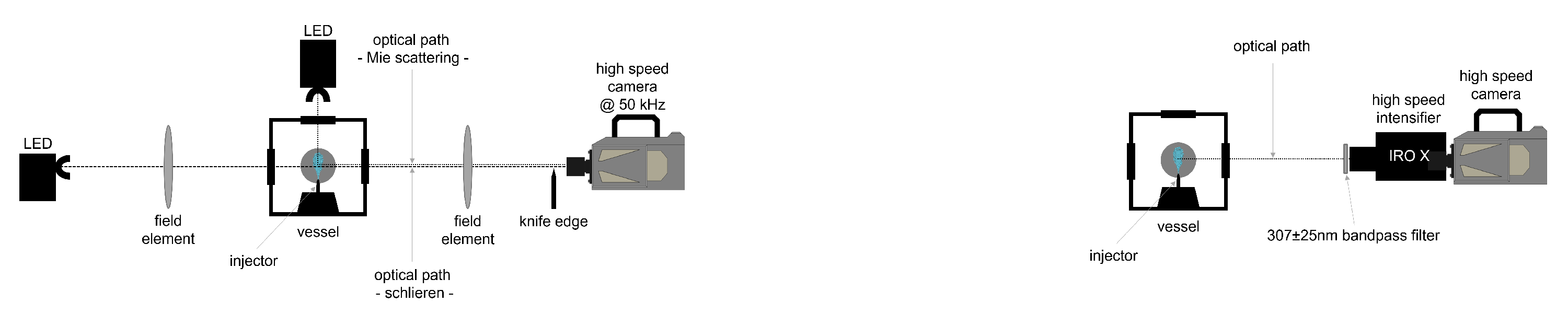
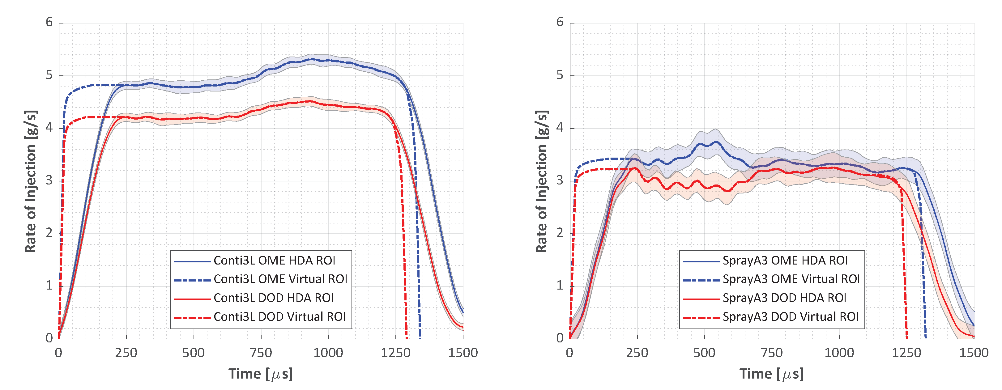
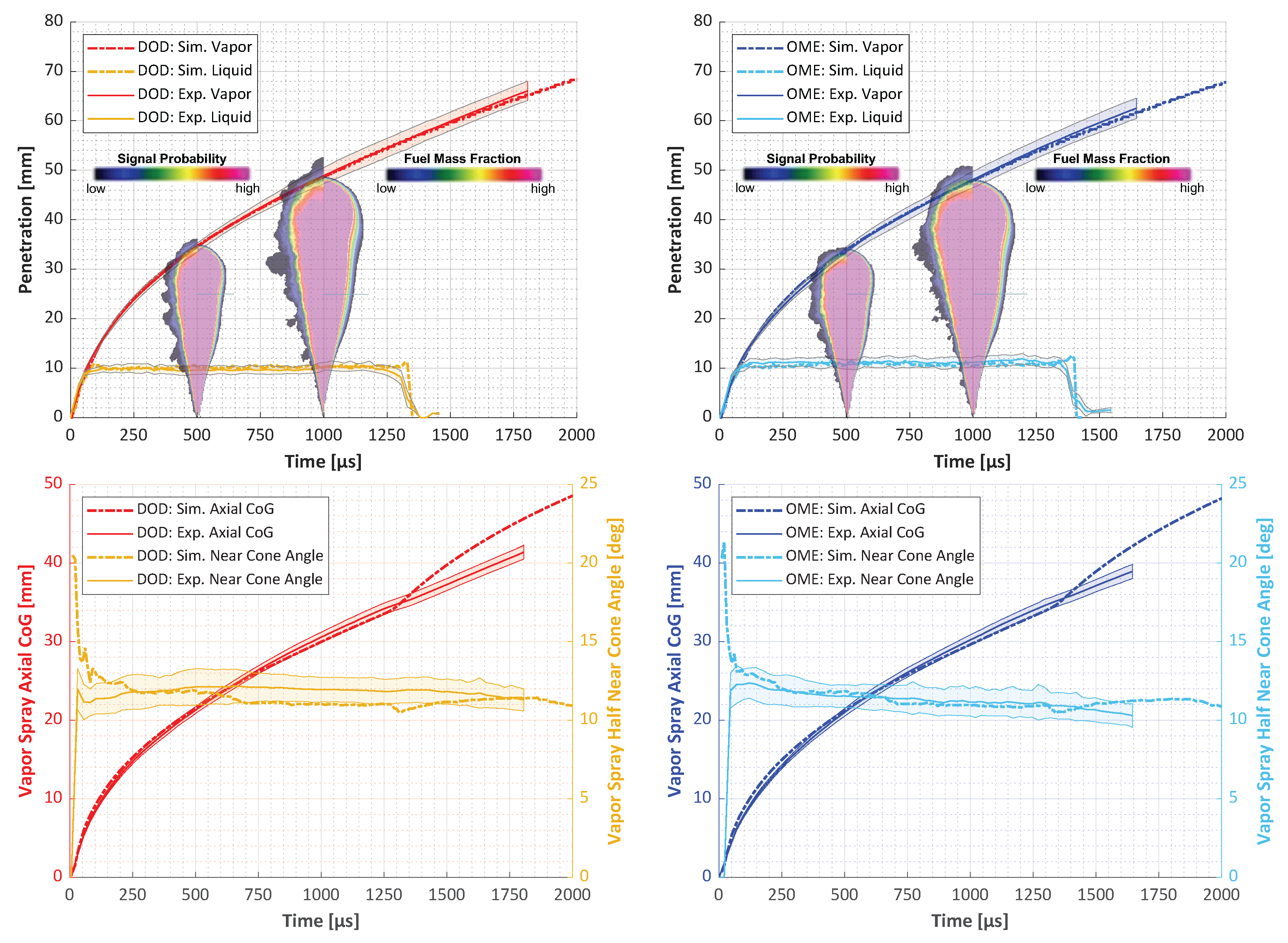
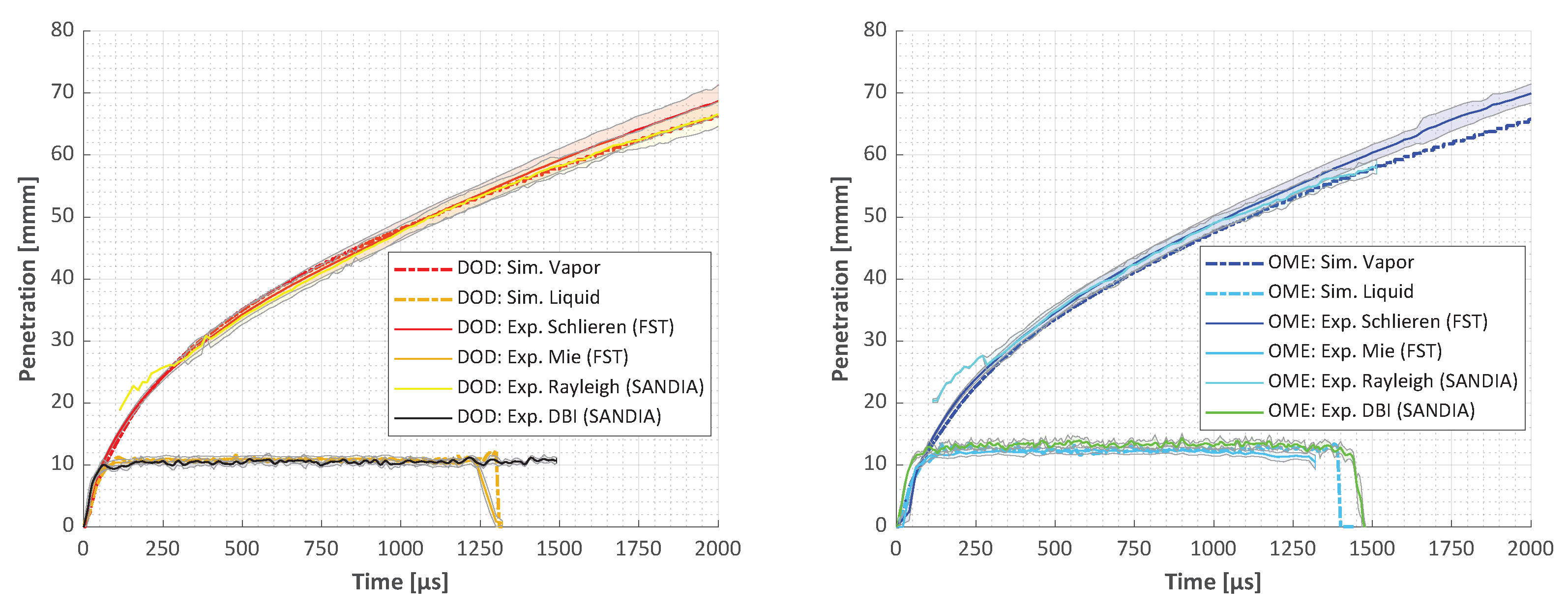
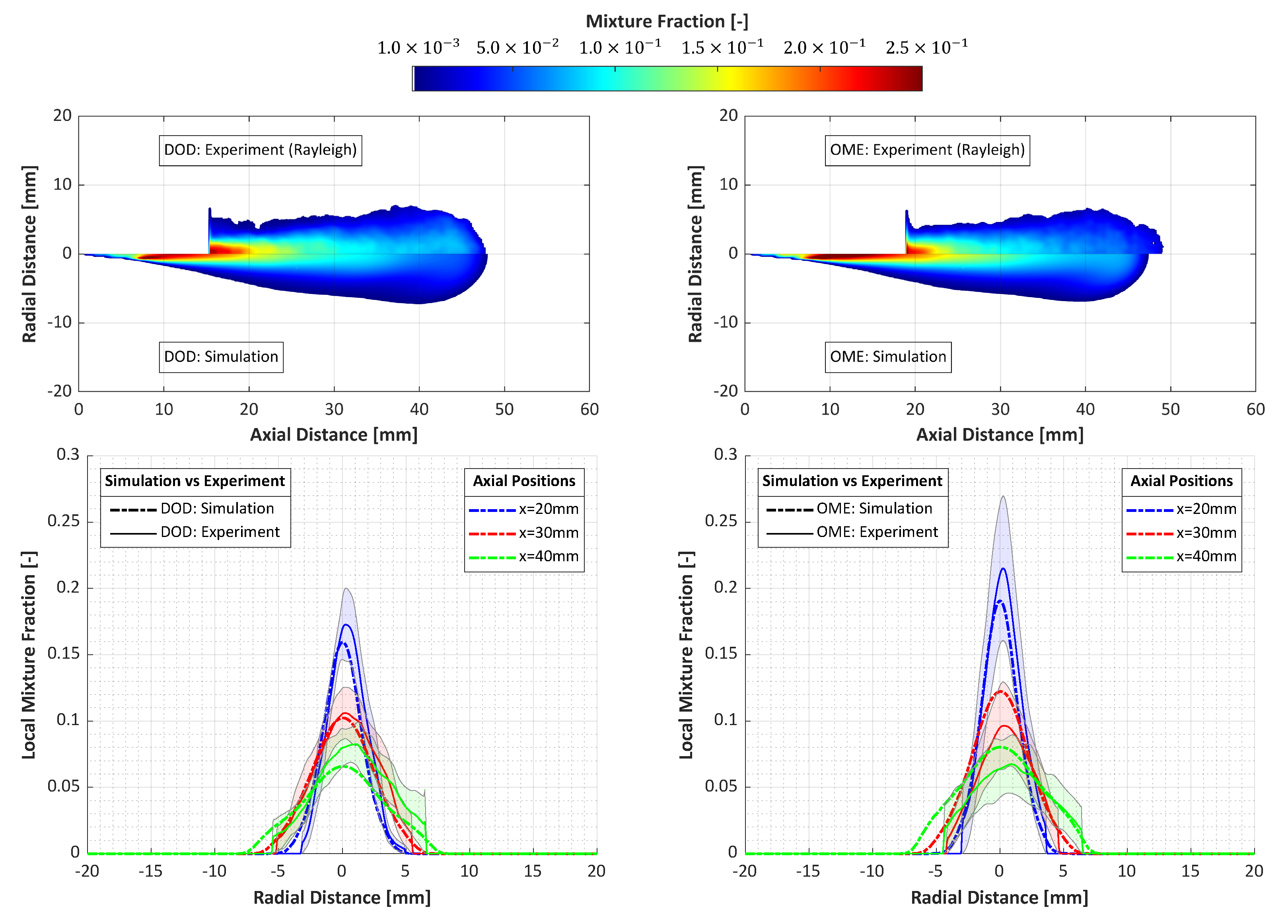
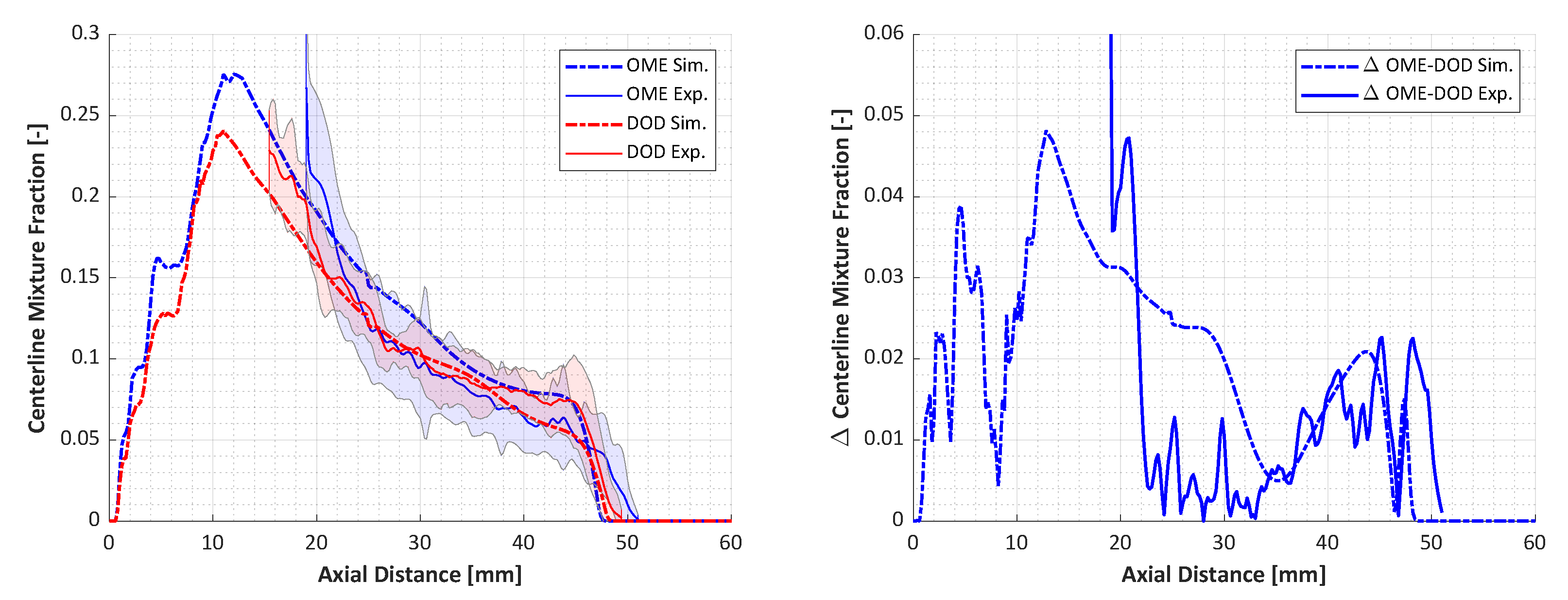
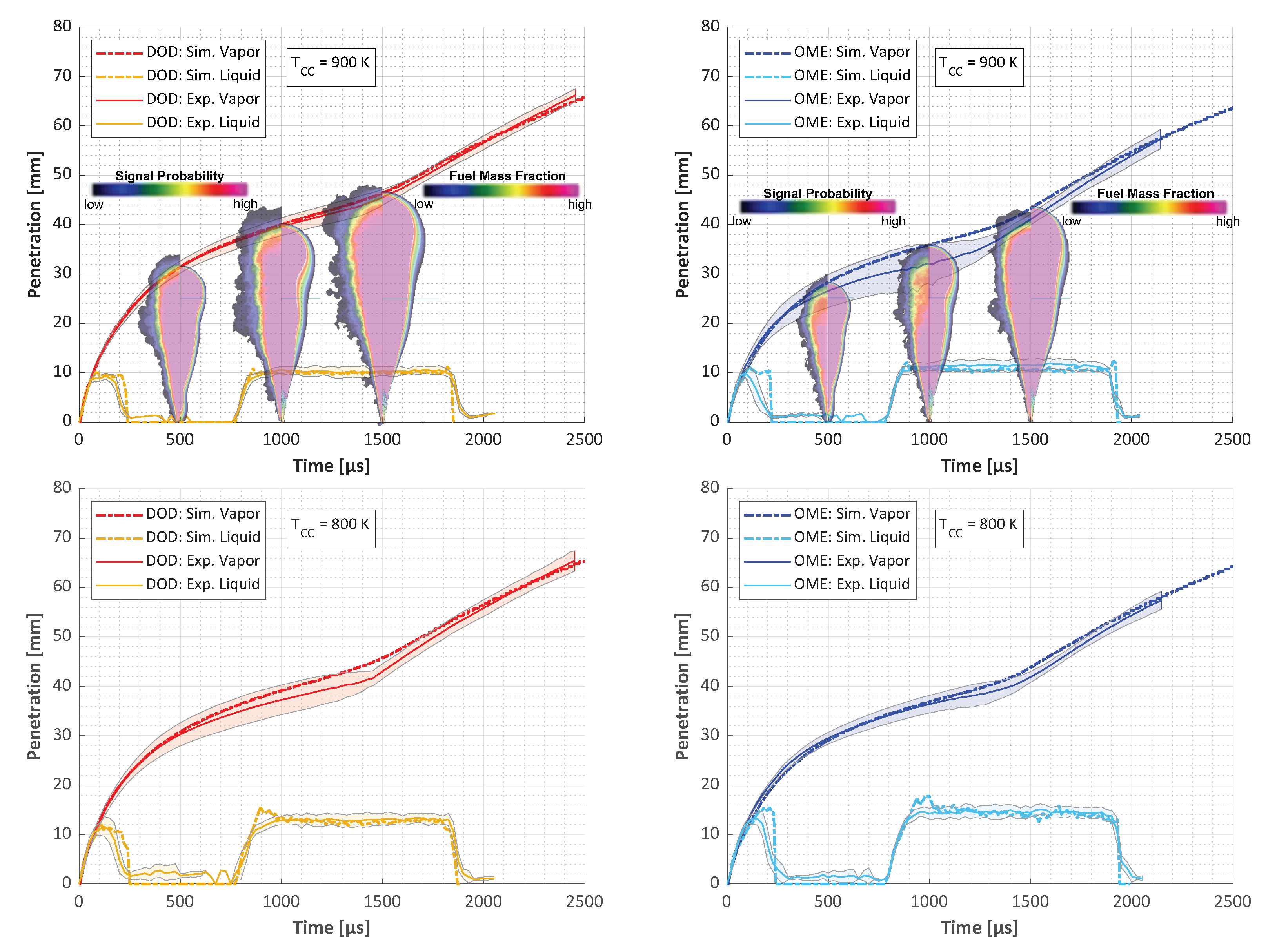
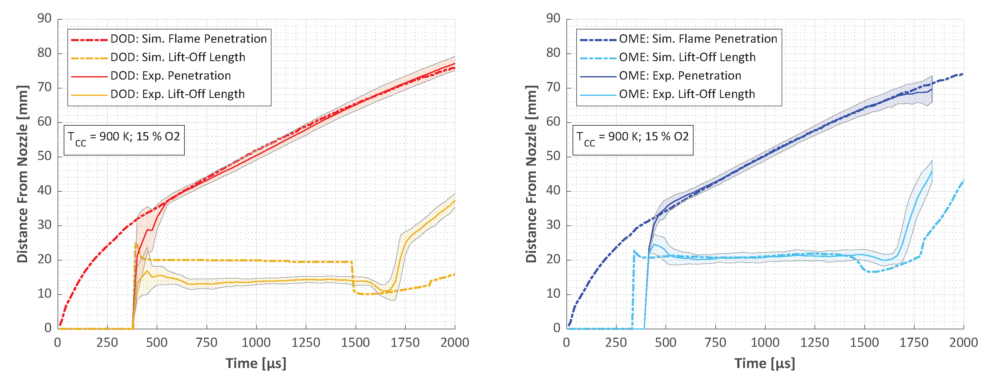
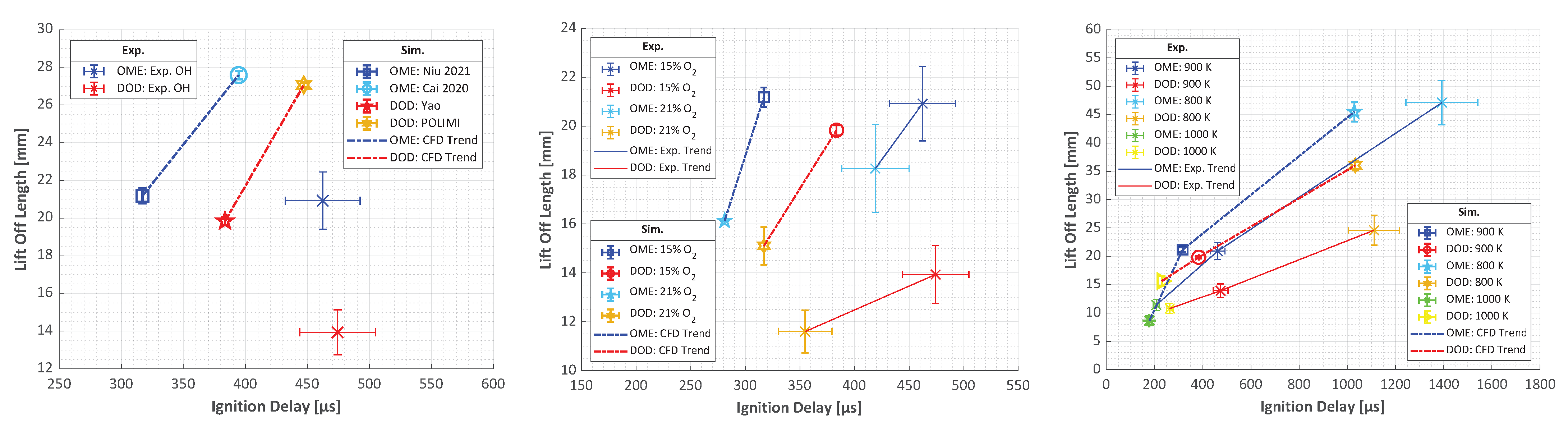
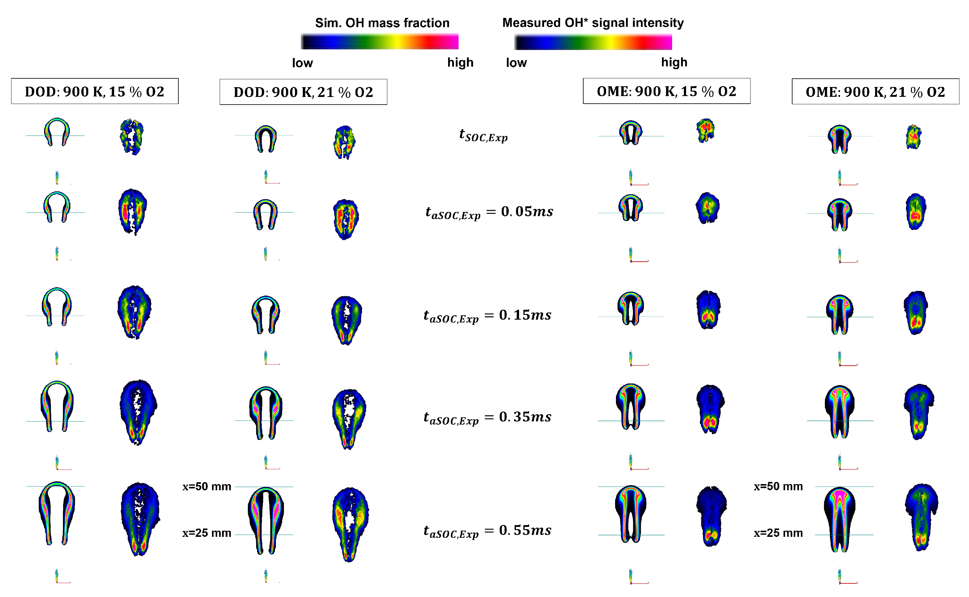
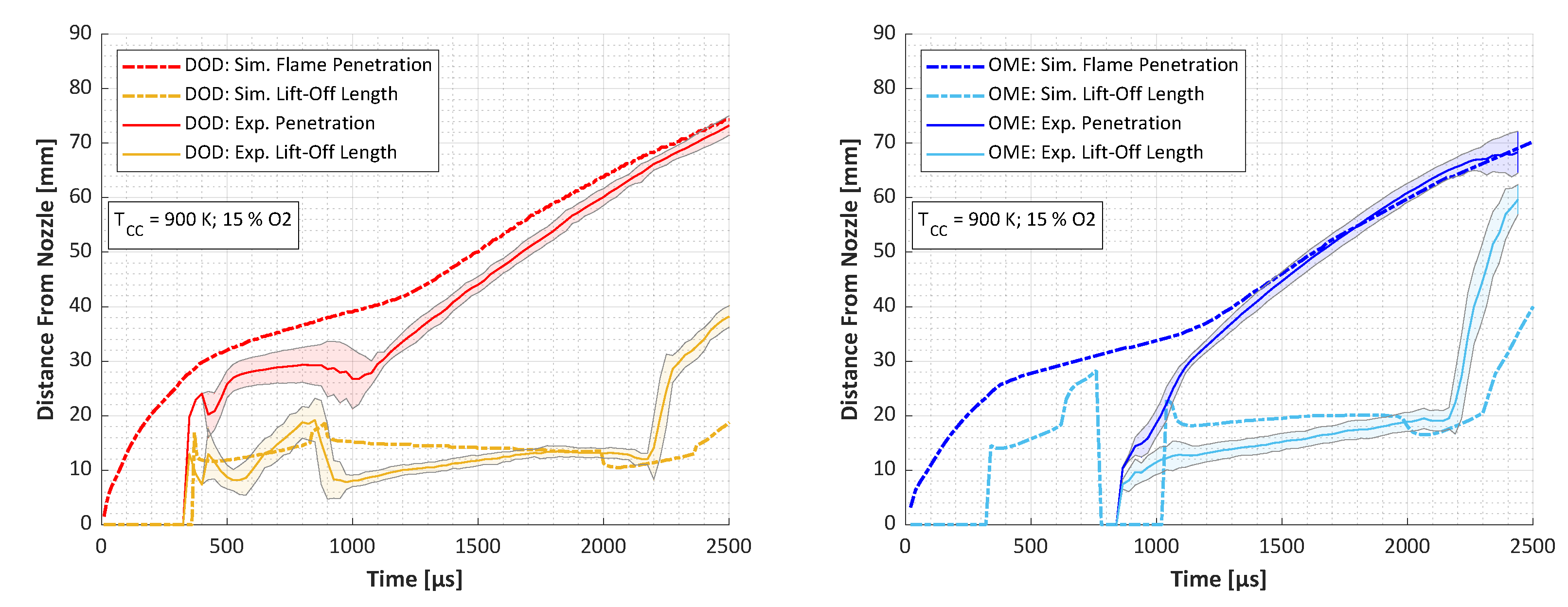
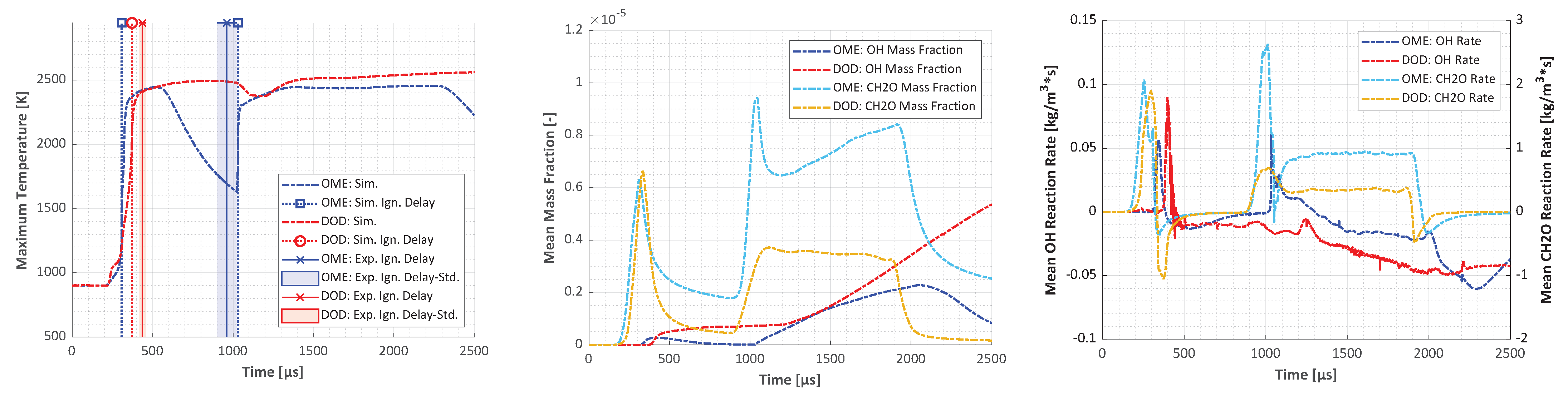
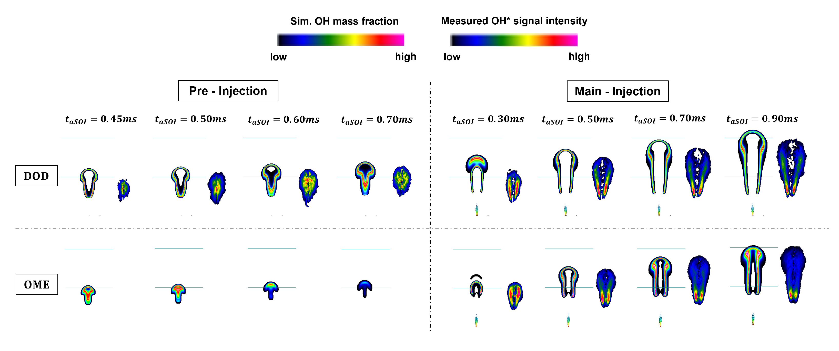
Table 1.
OME mix composition.
| Molecule | Content [wt %] |
|---|---|
| OME | 0.01 |
| OME | <0.01 |
| OME | 57.90 |
| OME | 28.87 |
| OME | 10.07 |
| OME | 1.91 |
Table 2.
Fuel properties for dodecane and OME.
| Property | Unit | Dodecane | OME |
|---|---|---|---|
| Density | kg/m (T = 15 C) | 751.20 | 1057.10 |
| Viscosity | mm/s (T = 40 C) | 1.44 | 1.08 |
| Cetane number | - | 74 | 68.6 |
| Lubricity | 563 | 320 | |
| Flash point | C | 83 | 65 |
| Lower heating value | MJ/kg | 44.20 | 19.26 |
| Initial boiling point | C | 214.00 | 144.40 |
| Final boiling point | C | 218 | 242.4 |
| Total contaminations | mg/kg | - | <1 |
| Carbon content | % [m/m] | 84 | 43 |
| Hydrogen content | % [m/m] | 16 | 8.53 |
| Oxygen content | % [m/m] | 0 | 46.4 |
| (A/F) at 21% of O | - | 14.92:1 | 5.89:1 |
| (A/F) at 15% of O | - | 20.72:1 | 8.18:1 |
Table 3.
Injector properties.
| Conti3L | SprayA3 | |
|---|---|---|
| Orifice exit diameter [] | 115 | 97 |
| Contraction coefficient [-] | 0.98 | 0.98 |
| Number of holes [-] | 3 | 1 |
| Elevation angle [] | 45 | 0 |
Table 4.
Operating points.
| Name | T [K] | p [bar] | [kg/m] | T [K] | p [bar] | t [ms] | O-Content [vol. %] |
|---|---|---|---|---|---|---|---|
| T2i | 800 | 55 | 22.8 | 363 | 1500 | 1.5 | 0 |
| T2r | 800 | 54 | 22.8 | 363 | 1500 | 1.5 | 15 |
| T2iM | 800 | 55 | 22.8 | 363 | 1500 | 0.3/0.5/1.2 | 0 |
| T2rM | 800 | 54 | 22.8 | 363 | 1500 | 0.3/0.5/1.2 | 15 |
| Ai | 900 | 62 | 22.8 | 363 | 1500 | 1.5 | 0 |
| Ar | 900 | 61 | 22.8 | 363 | 1500 | 1.5 | 15 |
| AiM | 900 | 62 | 22.8 | 363 | 1500 | 0.3/0.5/1.2 | 0 |
| ArM | 900 | 61 | 22.8 | 363 | 1500 | 0.3/0.5/1.2 | 15 |
| O2 | 900 | 60 | 22.8 | 363 | 1500 | 1.5 | 21 |
| T3i | 1000 | 69 | 22.8 | 363 | 1500 | 1.5 | 0 |
| T3r | 1000 | 68 | 22.8 | 363 | 1500 | 1.5 | 15 |
Table 5.
Mesh refinements.
| Refinement | L [mm] | R1 [mm] | R2 [mm] | Cell Size [mm] |
|---|---|---|---|---|
| 0 (Base Mesh) | 120 | 30 | 30 | 1.000 |
| 1 | 80 | 5 | 10 | 0.500 |
| 2 | 50 | 3 | 5 | 0.250 |
| 3 | 25 | 2 | 3 | 0.125 |
Table 6.
Summary of Eulerian numerical setup.
| Meshing | |
|---|---|
| Type | Cylindrical spray-box |
| Cell refinement | 1 mm–0.125 mm |
| Dimensions | Length = 120 mm; Diameter = 60 mm |
| Boundaries | Fixed temperature walls; non-reflecting outlet |
| Gaseous phase models | |
| Temporal discretization | (during injection); (after injection) |
| Turbulence modeling | RANS approach; k--f model |
| Wall treatment | Compound (hybrid) |
| Pressure-correction | SIMPLE (1st) / PISO (2nd) |
Table 7.
KHRT breakup model parameters.
| Parameter | Value | Description |
|---|---|---|
| C | 0.61 | Parameter for stable child droplet radius |
| C | 8.5 (Conti3L) | Parameter for child droplet breakup time |
| 10 (SprayA3) | ||
| C | 10 | Parameter to only undergo KH breakup near the nozzle |
Table 8.
Summary of Lagrangian numerical setup.
| Liquid Spray Submodels | |
|---|---|
| Injection type | Blob |
| Breakup | KHRT |
| Turbulent dispersion | O’Rourke |
| Evaporation | Brenn et al. (Multi-Component) |
| Drag Law | Schiller-Naumann |
Table 9.
Conti3L: Inert liquid length results for OME and dodecane.
| Fuel | T [K] | Liquid Length Simulation [mm] | Liquid Length Experiment [mm] | Relative Simulation Error [%] |
|---|---|---|---|---|
| OME | 800 | 14.08 | 15.20 | −7.38 |
| 900 | 10.78 | 11.11 | −2.94 | |
| Dodecane | 800 | 13.07 | 12.59 | 3.86 |
| 900 | 10.19 | 9.70 | 5.06 |
Table 10.
Conti3L: Ignition delay and lift-off length results for OME (mechanism: Niu [45]) and dodecane (mechanism: Yao [42]).
| Fuel | T [K] | Oxygen Content [%] | Ignition Delay Sim. [s] | Ignition Delay Exp. [s] | Lift-Off Length Sim. [mm] | Lift-Off Length Exp. [mm] |
|---|---|---|---|---|---|---|
| OME | 800 | 15 | 1029 | 1392 | 45.50 | 47.12 |
| 900 | 15 | 317 | 462 | 21.18 | 20.92 | |
| 900 | 21 | 281 | 419 | 16.13 | 18.27 | |
| 1000 | 15 | 179 | 207 | 8.64 | 11.41 | |
| Dodecane | 800 | 15 | 1033 | 1111 | 36.04 | 24.61 |
| 900 | 15 | 384 | 474 | 19.84 | 13.93 | |
| 900 | 21 | 317 | 355 | 15.10 | 11.60 | |
| 1000 | 15 | 231 | 263 | 15.64 | 10.80 |
Publisher’s Note: MDPI stays neutral with regard to jurisdictional claims in published maps and institutional affiliations. |
© 2022 by the authors. Licensee MDPI, Basel, Switzerland. This article is an open access article distributed under the terms and conditions of the Creative Commons Attribution (CC BY) license (https://creativecommons.org/licenses/by/4.0/).
Share and Cite
MDPI and ACS Style
Wiesmann, F.; Strauß, L.; Rieß, S.; Manin, J.; Wan, K.; Lauer, T. Numerical and Experimental Investigations on the Ignition Behavior of OME. Energies 2022, 15, 6855. https://doi.org/10.3390/en15186855
AMA Style
Wiesmann F, Strauß L, Rieß S, Manin J, Wan K, Lauer T. Numerical and Experimental Investigations on the Ignition Behavior of OME. Energies. 2022; 15(18):6855. https://doi.org/10.3390/en15186855
Chicago/Turabian StyleWiesmann, Frederik, Lukas Strauß, Sebastian Rieß, Julien Manin, Kevin Wan, and Thomas Lauer. 2022. "Numerical and Experimental Investigations on the Ignition Behavior of OME" Energies 15, no. 18: 6855. https://doi.org/10.3390/en15186855
Note that from the first issue of 2016, this journal uses article numbers instead of page numbers. See further details here.