Heat to Hydrogen by Reverse Electrodialysis—Using a Non-Equilibrium Thermodynamics Model to Evaluate Hydrogen Production Concepts Utilising Waste Heat

Abstract

The reverse electrodialysis heat engine (REDHE) is a promising salinity gradient energy technology, capable of producing hydrogen with an input of waste heat at temperatures below 100 °C. A salinity gradient drives water electrolysis in the reverse electrodialysis (RED) cell, and spent solutions are regenerated using waste heat in a precipitation or evaporation unit. This work presents a non-equilibrium thermodynamics model for the RED cell, and the hydrogen production is investigated for KCl/water solutions. The results show that the evaporation concept requires 40 times less waste heat and produces three times more hydrogen than the precipitation concept. With commercial evaporation technology, a system efficiency of 2% is obtained, with a hydrogen production rate of 0.38 g${}_{{\mathrm{H}}_2}$ m${}^{-2}$h${}^{-1}$ and a waste heat requirement of 1.7 kWh g${}_{{\mathrm{H}}_2}^{-1}$. The water transference coefficient and the salt diffusion coefficient are identified as membrane properties with a large negative impact on hydrogen production and system efficiency. Each unit of the water transference coefficient in the range $t_w=\left[0–10\right]$ causes a −7 mV decrease in unit cell electric potential, and a −0.3% decrease in system efficiency. Increasing the membrane salt diffusion coefficient from 10${}^{-12}$ to 10${}^{-11}$ leads to the system efficiency decreasing from 2% to 0.6%.

1. Introduction

To enable the transition from fossil fuels to renewable fuels, more renewable energy sources need to be exploited and the capacity for energy storage must increase dramatically. Salinity gradient energy has gained increasing attention in the last years due to the large theoretical potential that lies in the mixing of fresh- and seawater (estimated to be between 1.4 and 2.6 TW for the worldwide discharge of river water and the average sea salinity [1]). The chemical potential difference between a high-salinity and a low-salinity stream can be harvested as electric energy by controlled mixing across ion-exchange membranes. Neighbouring compartments of concentrate and dilute electrolytes are separated by alternating cation- and anion-exchange membranes (AEMs/CEMs). A net flux of ions arises across the membranes and the ionic current is converted to electric current by electrodes at each side of the stack [2,3]. This concept is known as reverse electrodialysis (RED), as illustrated in Figure 1.

The concept of converting salinity gradients to energy by mixing fresh and saltwater was first introduced by Pattle in the 1950s [4]. Loeb patented the method and apparatus for a heat engine using pressure retarded osmosis (PRO) in 1975 [5], and for a heat engine using RED with a thermal regeneration unit in 1979 [6]. A prototype for RED power generation from natural saturated brines from salt ponds and brackish water was commissioned in 2014 in Italy with a total membrane area of almost 50 ${\mathrm{m}}^2$ and a power output of 40 W [7,8]. By using saturated brines as high-concentration and brackish water as low-concentration feed streams, the electrical resistance of the dilute compartment was decreased compared to using freshwater, and a higher power output can be achieved [9,10,11,12,13]. However, this concept depends on readily available solutions of different salinity found close together in the environment.

By coupling a RED unit with a thermal regeneration unit that restores the initial concentrations of the concentrate and dilute feed streams, a closed-loop heat engine can be obtained: the reverse electrodialysis heat engine (REDHE). Due to the regeneration of the electrolyte, only a finite amount of salt solution is needed, which allows for flexibility in the system’s location and the choice of salt. Consequently, the electrolyte can be selected based on its thermodynamic and transport properties, ensuring satisfactory energy conversion from the available heat.

The electrical current generated from the REDHE may also be used for green hydrogen production. Hydrogen is acknowledged as a promising energy storage technology and may serve as a viable substitute for diesel and gasoline, given that safe procedures for handling are in place [14,15,16,17,18]. Hydrogen has a yearly production of around 500 billion ${\mathrm{m}}^3$, of which roughly 96% is produced using fossil fuels, in particular through steam reforming of methane [15,19,20,21,22,23]. REDHE could be exploited for direct renewable hydrogen production, where the hydrogen gas can be considered carbon-neutral [24]. By utilising industrial waste heat for the solution regeneration, a readily available energy source is exploited instead of grid-based energy, and the overall energy efficiency of existing production cycles is enhanced [25]. Relevant regeneration concepts are illustrated in Figure 2 and Figure 3.

Industrial processes are irreversible, and a significant fraction of the input energy is dissipated as waste heat to the ambient environment. Chemical, petrochemical and metal production processes are relevant examples [26,27,28,29]. The thermal energy is transported from industrial equipment and products to surroundings by conduction, convection and radiation. The majority of industrial waste heat is released at low temperatures. In 2007, in the USA around 1358 TWh of waste heat was released at temperatures between 50 and 99 °C [30], and in Germany, around 44 TWh of recoverable waste heat from big industrial plants was released at temperatures between 60–140 °C [31]. Existing mature technologies for waste heat utilisation are mainly limited to high- and medium-temperature waste heat (around 100 to 650 °C) because the conversion of low-temperature waste heat to electricity does not reach sufficient efficiencies for industrial use [32]. Papapetrou et al. estimated the recoverable part of waste heat from main industrial sectors in the EU based on Eurostat data from 2015 and found a recoverable potential of roughly 300 TWh/year with around one-third in the temperature range of 100–200 °C [29].

The REDHE can use low-temperature waste heat for the production of electricity or hydrogen [32]. To reach sufficient efficiencies for the industrialisation of the technology, both ion-exchange membranes and process design need to be optimised [33]. Optimisation potentials have been elaborated in previous investigations on REDHE for electricity generation [34,35,36,37,38], and for hydrogen production [24,39,40,41]. The choice of electrolyte composition, regeneration technology and ion-exchange membrane performance have been identified as particularly important influencing factors [32,39,42].

However, there is a need to assess the membrane transport phenomena i.e., coupling between the fluxes of water, salt and charge. Such coupling may have an impact on the overall efficiency of the system and is known to affect the membrane permselectivity in a manner that is typically not accounted for in REDHE models [43]. Models of higher complexity may be necessary to investigate the effect of key parameters, and to identify the most promising RED and regeneration concepts [33]. This work will expand on previous descriptions of the REDHE by using the framework of non-equilibrium thermodynamics to describe the fluxes of water and salt through ion-exchange membranes in a RED cell producing hydrogen [44]. Mass and energy balances will also be solved for flow parallel to membranes in the RED cell, and for the regeneration unit using waste heat. Furthermore, a precipitation and evaporation concept, described previously by Krakhella et al. [39] and Tamburini et al. [32], are investigated for electrolyte regeneration. The system will be assessed as a whole with a focus on the RED cell parameters.

2. Theory

2.1. Outline

The framework of non-equilibrium thermodynamics is used to describe component fluxes in the direction orthogonal to the ion-exchange membranes, in a cell with counter-current convective solution flow parallel to the membranes [44]. Viscous dissipation is neglected for all flows in the system. The reverse electrodialysis (RED) cell has compartments of aqueous electrolyte solutions of alternating concentrations, separated by alternating anion- and cation-exchange membranes (AEM and CEM, respectively), as illustrated in Figure 1. Electrode compartments are filled with a circulating alkaline solution, but are here only treated as a solution of the monovalent salt M${}^{+}$X${}^{-}$ of molality equal to the average of the concentrate and dilute molalities. Metallic electrodes facilitate the alkaline electrolysis of water in the anode and cathode compartments. The electrode reactions are:

$$\begin{array}{cc}\hfill \mathrm{Anode}:& {\mathrm{OH}}^{-}\to \frac{1}{2}{\mathrm{H}}_2\mathrm{O}+\frac{1}{4}{\mathrm{O}}_2+{\mathrm{e}}^{-}\hfill \\ \hfill \mathrm{Cathode}:& {\mathrm{H}}_2\mathrm{O}+{\mathrm{e}}^{-}\to \frac{1}{2}{\mathrm{H}}_2+\mathrm{O}{\mathrm{H}}^{-}\hfill \\ \hfill \mathrm{Total}:& \frac{1}{2}{\mathrm{H}}_2\mathrm{O}\left(\mathrm{l}\right)\to \frac{1}{2}{\mathrm{H}}_2\left(\mathrm{g}\right)+\frac{1}{4}{\mathrm{O}}_2\left(\mathrm{g}\right)\hfill \end{array}$$

The total electric potential difference from the anode to the cathode is given by the sum of potential differences across phases and interfaces:

$$\begin{array}{cc}\hfill \mathsf{\Delta }{\varphi }_{\mathrm{tot}}=& {\varphi }_c-{\varphi }_a\hfill \\ \hfill =& \mathsf{\Delta }{\varphi }_a+{\mathsf{\Delta }}_{a,r}\varphi +\mathsf{\Delta }{\varphi }_r+{\mathsf{\Delta }}_{r,1}{\varphi }^{\mathrm{CEM}}+\mathsf{\Delta }{\varphi }_1+N\mathsf{\Delta }{\varphi }_{\mathrm{unit}}\hfill \\ \hfill & +{\mathsf{\Delta }}_{1,2}{\varphi }^{\mathrm{AEM}}+\mathsf{\Delta }{\varphi }_2+{\mathsf{\Delta }}_{2,r}{\varphi }^{\mathrm{CEM}}+\mathsf{\Delta }{\varphi }_r+{\mathsf{\Delta }}_{r,c}\varphi +\mathsf{\Delta }{\varphi }_c\hfill \end{array}$$

(1)

where subscripts a, r, 1, 2 and c are the anode, rinse solution, dilute electrolyte solution, concentrate electrolyte solution and cathode phases, respectively. The combination of subscripts gives the difference across the surfaces ${\mathsf{\Delta }}_{i,o}\varphi ={\varphi }_o-{\varphi }_i$ (out of minus into the surface) [44]. The unit cell is a repeating portion of the RED cell, for which the electric potential difference is:

$$\mathsf{\Delta }{\varphi }_{\mathrm{unit}}=\mathsf{\Delta }{\varphi }_1+{\mathsf{\Delta }}_{1,2}{\varphi }^{\mathrm{AEM}}+\mathsf{\Delta }{\varphi }_2+{\mathsf{\Delta }}_{2,1}{\varphi }^{\mathrm{CEM}}$$

(2)

and the total emf contribution is proportional to the number, N, of such repeating portions. Superscripts CEM and AEM denote the membrane phases. In our treatment of the isothermal RED cell, we assume that all electrolyte and rinse solutions are perfectly mixed, such that there is no concentration polarisation. As a result, the electric potential contributions from the solution flow compartments are exclusively ohmic, and concentration gradients are confined to the membrane phases. Additionally, we assume electrochemical equilibrium at the interfaces between flow compartments and membranes (Donnan equilibrium), such that there are no net electric potential contributions from each of the membrane interfaces, only from the gradients across the whole membrane [44].

2.2. Contribution from the Electrodes

The fluxes of species into and out of the electrode surfaces are directly related to the current density through the reaction stoichiometry, and in a steady state we express the isothermal electrode surface entropy production by:

$${\sigma }^s=-\frac{j}{T}\left({\mathsf{\Delta }}_{i,o}\varphi +\frac{{\mathsf{\Delta }}_n{G}_s}{F}\right)$$

(3)

where j is the current density, T is the temperature, F is Faraday’s constant, ${\mathsf{\Delta }}_n{G}_s$ is the reaction Gibbs energy of the neutral components and ${\mathsf{\Delta }}_{i,o}\varphi$ is the electric potential difference across the surface [44,45]. The corresponding flux equation for the surface is:

$$-\left({\mathsf{\Delta }}_{i,o}\varphi +\frac{{\mathsf{\Delta }}_n{G}_s}{F}\right)=R_{s}j$$

(4)

where $R_s$ is a surface resistance related to the activation overpotential through: $\eta =|{\mathsf{\Delta }}_{i,o}\varphi -{\mathsf{\Delta }}_{i,o}{\varphi }_{j\to 0}|$. For the anode ${\mathsf{\Delta }}_n{G}^{s,a}=\frac{1}{4}{\mu }_{{\mathrm{O}}_2}+\frac{1}{2}{\mu }_{{\mathrm{H}}_2\mathrm{O}}$, and for the cathode ${\mathsf{\Delta }}_n{G}^{s,c}=\frac{1}{2}{\mu }_{{\mathrm{H}}_2}-{\mu }_{{\mathrm{H}}_2\mathrm{O}}$, where ${\mu }_k$ is the chemical potential of component k at constant temperature. The sum of the anode and cathode contributions leads to:

$${\mathsf{\Delta }}_{a,r}\varphi +{\mathsf{\Delta }}_{r,c}\varphi =-\frac{{\mathsf{\Delta }}_n{G}_{\mathrm{tot}}}{F}-\eta$$

(5)

where the first term on the right-hand side is the electric potential for water electrolysis at standard temperature and pressure, −1.23 V. Contributions from the electrode bulk phases and connecting leads, $\mathsf{\Delta }{\varphi }_a$ and $\mathsf{\Delta }{\varphi }_c$, are taken as ohmic contributions and are here included in the overpotential as a simplification. Hydrogen and oxygen production and water consumption are related to the current density through:

$$F_{{\mathrm{H}}_2}=\frac{j{M}_{{\mathrm{H}}_2}}{2F},F_{{\mathrm{O}}_2}=\frac{j{M}_{{\mathrm{O}}_2}}{4F},F_{{\mathrm{H}}_2\mathrm{O}}=-\frac{j{M}_{{\mathrm{H}}_2\mathrm{O}}}{2F}$$

(6)

Here, $M_k$ is the molecular weight and $F_k$ is the production or consumption of component k. The rinse solutions must therefore be continuously refilled with water.

2.3. Contribution from the Rinse Solutions

We take the rinse solution to be of constant composition throughout its cycle between anode and cathode. The entropy production of the CEMs in contact with the rinse solution can then be written as:

$${\sigma }^m=-J_e\frac{{\mathsf{\Delta }}_{i,o}{\mu }_e}{T}-J_w\frac{{\mathsf{\Delta }}_{i,o}{\mu }_w}{T}-j\frac{{\mathsf{\Delta }}_{i,o}\varphi }{T}$$

(7)

where ${\mu }_e$ and ${\mu }_w$ are the chemical potentials of electrolyte and water and $J_e$ and $J_w$ are molar fluxes of electrolyte and water respectively. The corresponding flux equations for a membrane are:

$$\left[\begin{array}{c}{J}_e\\ J_w\\ j\end{array}\right]=\left[\begin{array}{ccc}{L}_{ee}& L_{ew}& L_{e\varphi }\\ L_{we}& L_{ww}& L_{w\varphi }\\ L_{\varphi e}& L_{\varphi w}& L_{\varphi \varphi }\end{array}\right]\left[\begin{array}{c}-T^{-1}{\mathsf{\Delta }}_{i,o}{\mu }_e\\ -T^{-1}{\mathsf{\Delta }}_{i,o}{\mu }_w\\ -T^{-1}{\mathsf{\Delta }}_{i,o}\varphi \end{array}\right]$$

(8)

where $L_{ij}$ are phenomenological transport coefficients. These coefficients may vary with concentration of salt but are here assumed constant, and we use differences instead of derivatives. Continuing with the current density and rearranging with respect to the electric potential gives:

$${\mathsf{\Delta }}_{i,o}\varphi =-\frac{L_{\varphi e}}{L_{\varphi \varphi }}{\mathsf{\Delta }}_{i,o}{\mu }_e-\frac{L_{\varphi w}}{L_{\varphi \varphi }}{\mathsf{\Delta }}_{i,o}{\mu }_w-\frac{T}{L_{\varphi \varphi }}j$$

(9)

The electrolyte flux is not a local flux of aqueous M${}^{+}$X${}^{-}$ in one direction, but rather a net transfer of electrolyte between compartments due to the sum of local ionic fluxes [45,46]. Furthermore, the relationship between the electrolyte flux and the local fluxes of anions and cations depends on the electrode reactions [47]. The salt transference number is an important property when describing the membrane transport, as it quantifies the net amount of salt which is reversibly transported with the electric current:

$$\begin{array}{c}\hfill t_e=F\frac{L_{\varphi e}}{L_{\varphi \varphi }}=F{\left(\frac{J_e}{j}\right)}_{\mathrm{d}\mu =0}\end{array}$$

(10)

where $t_e$ is the salt transference number, and the Onsager relation, $L_{ij}=L_{ji}$, was used [44]. The remaining phenomenological coefficients of Equation (9) are:

$$\begin{array}{cc}\hfill t_w& =F\frac{L_{\varphi w}}{L_{\varphi \varphi }}=F{\left(\frac{J_w}{j}\right)}_{\mathrm{d}\mu =0}\hfill \\ \hfill R_s& =\frac{T}{L_{\varphi \varphi }}={\left(\frac{{\mathsf{\Delta }}_{i,o}\varphi }{j}\right)}_{\mathrm{d}\mu =0}\hfill \end{array}$$

(11)

where $t_w$ is the water transference number i.e., the moles of water transported reversibly per Coulomb of current, and $R_s$ is the area electric resistance of the phase s. The electric potential difference across the membrane becomes:

$${\mathsf{\Delta }}_{i,o}\varphi =-\frac{t_e}{F}{\mathsf{\Delta }}_{i,o}{\mu }_e-\frac{t_w}{F}{\mathsf{\Delta }}_{i,o}{\mu }_w-R_{s}j$$

(12)

Once again using the assumption of constant solution composition in the rinse solution circulated between anode and cathode, the contribution from each bulk rinse solution is: $\mathsf{\Delta }{\varphi }_r=-R_{r}j$. Furthermore, due to this assumption, we find that the sum of contributions from the two CEMs in contact with rinse solutions is:

$${\mathsf{\Delta }}_{r,1}{\varphi }^{\mathrm{CEM}}+{\mathsf{\Delta }}_{2,r}{\varphi }^{\mathrm{CEM}}=-\frac{t_e}{F}{\mathsf{\Delta }}_{2,1}{\mu }_e-\frac{t_w}{F}{\mathsf{\Delta }}_{2,1}{\mu }_w-2R^{\mathrm{CEM}}j$$

(13)

where the CEM resistance is considered constant and equal for all CEMs. It is convenient to introduce the membrane permselectivity:

$$\alpha =\pm \nu {\left(\frac{{\mathsf{\Delta }}_{i,o}\varphi }{{\mathsf{\Delta }}_{i,o}{\mu }_e/F}\right)}_{j=0}=\mp \nu \left(t_e+t_w\frac{{\mathsf{\Delta }}_{i,o}{\mu }_w}{{\mathsf{\Delta }}_{i,o}{\mu }_e}\right)$$

(14)

where the expression is multiplied by plus or minus the stoichiometric coefficient of the salt, $\nu$, due to the nature of the salt transference number for a RED stack given in Equation (10). In this cell, the salt transference number is 0.5 for a perfectly selective CEM and −0.5 for a perfect AEM, such that Equation (14) can be scaled by $+\nu$ for a CEM and $-\nu$ for an AEM in order to obtain positive permselectivity values in the range of 0 to 1. The chemical potential gradient of water may be calculated from activity coefficients using the Gibbs–Duhem equation and the definition of the osmotic coefficient [48]. Therefore, Equation (13) becomes:

$${\mathsf{\Delta }}_{r,1}{\varphi }^{\mathrm{CEM}}+{\mathsf{\Delta }}_{2,r}{\varphi }^{\mathrm{CEM}}={\alpha }^{\mathrm{CEM}}\frac{{\mathsf{\Delta }}_{1,2}{\mu }_e}{\nu F}-2R^{\mathrm{CEM}}j$$

(15)

where ${\alpha }^{\mathrm{CEM}}$ is the permselectivity of the CEMs in contact with the rinse solutions.

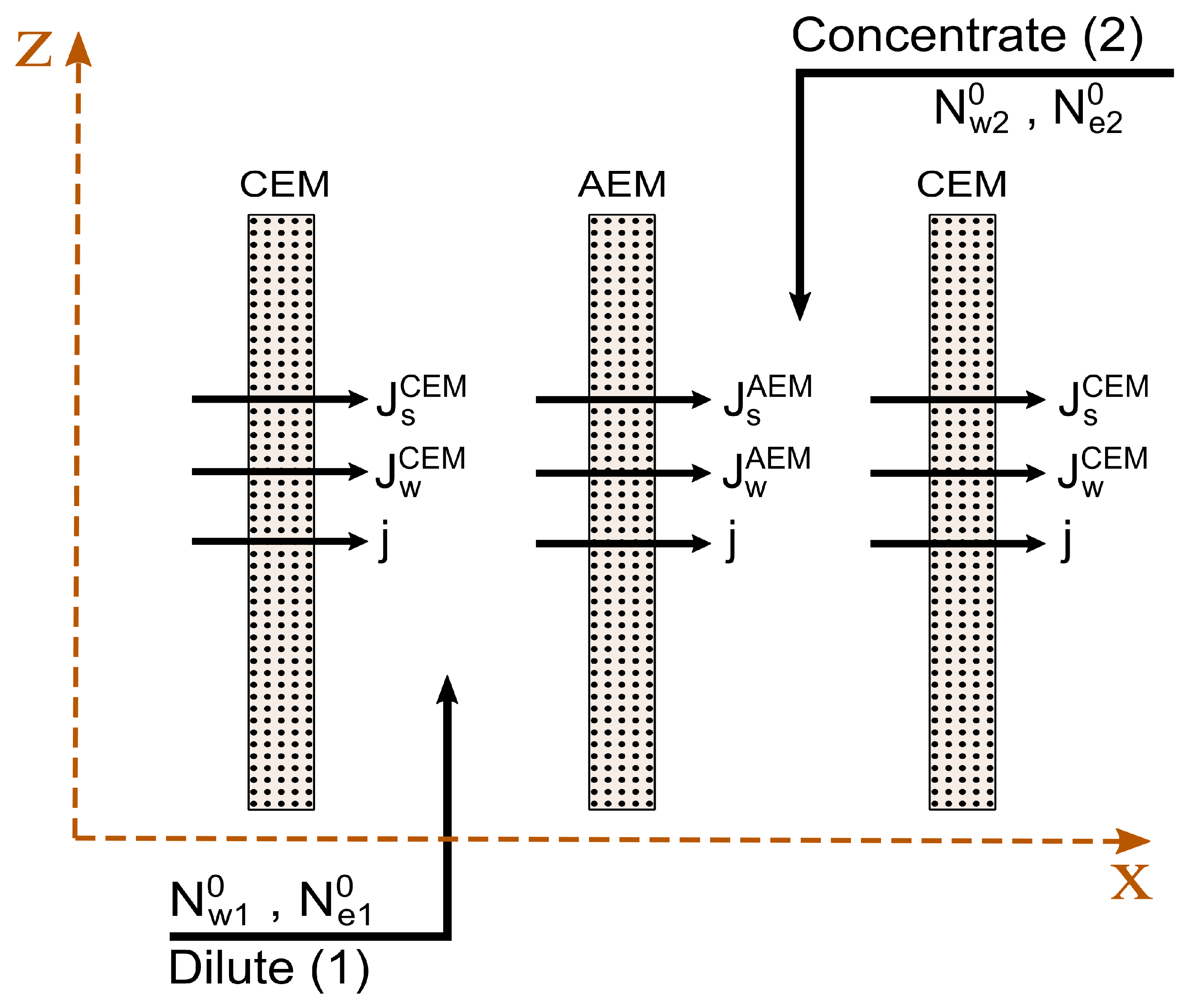
2.4. Contribution from a Unit Cell

Equation (12) holds for the remaining membranes as well, and may be combined with Equation (2) for one of the repeating unit cells resulting in:

$$\begin{array}{cc}\hfill \mathsf{\Delta }{\varphi }_{\mathrm{unit}}=& -\frac{t_e^{\mathrm{AEM}}}{F}{\mathsf{\Delta }}_{1,2}{\mu }_e-\frac{t_w^{\mathrm{AEM}}}{F}{\mathsf{\Delta }}_{1,2}{\mu }_w\hfill \\ \hfill & -\frac{t_e^{\mathrm{CEM}}}{F}{\mathsf{\Delta }}_{2,1}{\mu }_e-\frac{t_w^{\mathrm{CEM}}}{F}{\mathsf{\Delta }}_{2,1}{\mu }_w\hfill \\ & -(R^{\mathrm{AEM}}+R^{\mathrm{CEM}}+R_1+R_2)j\hfill \end{array}$$

(16)

which in terms of membrane permselectivities becomes:

$$\begin{array}{cc}\hfill \mathsf{\Delta }{\varphi }_{\mathrm{unit}}=& ({\alpha }^{\mathrm{AEM}}+{\alpha }^{\mathrm{CEM}})\frac{{\mathsf{\Delta }}_{1,2}{\mu }_e}{\nu F}\hfill \\ \hfill & -(R^{\mathrm{AEM}}+R^{\mathrm{CEM}}+R_1+R_2)j\hfill \end{array}$$

(17)

2.5. The Total Cell

In addition to the electrode compartments separated by CEMs already detailed, the base stack features one more AEM membrane such that the stack has one unit cell when $N=0$. In total, the potential drop across the cell is then:

$$\begin{array}{cc}\hfill \mathsf{\Delta }{\varphi }_{\mathrm{tot}}=& -\frac{{\mathsf{\Delta }}_n{G}_{\mathrm{tot}}}{F}-\eta +(N+1)({\alpha }^{\mathrm{AEM}}+{\alpha }^{\mathrm{CEM}})\frac{{\mathsf{\Delta }}_{1,2}{\mu }_e}{\nu F}\hfill \\ \hfill & -2(R^{\mathrm{CEM}}+R_r)j-(N+1)(R^{\mathrm{AEM}}+R^{\mathrm{CEM}}+R_1+R_2)j\hfill \\ \hfill =& -\frac{{\mathsf{\Delta }}_n{G}_{\mathrm{tot}}}{F}-\eta +{\left(\mathsf{\Delta }{\varphi }_{\mathrm{RED}}\right)}_{j=0}-R_{\mathrm{RED}}j\hfill \end{array}$$

(18)

where $\mathsf{\Delta }{\varphi }_{\mathrm{RED}}$ and $R_{\mathrm{RED}}$ are the total potential and resistance contributions from the RED stack.

2.6. Component Fluxes

Fluxes of water and salt through a membrane are also given by the flux–force relations in Equation (8). Introducing Equation (9) into the component fluxes and using the following substitution:

$$l_{ij}=L_{ij}-\frac{L_{i\varphi }{L}_{\varphi j}}{L_{\varphi \varphi }}$$

(19)

the molar component fluxes become:

$$\begin{array}{cc}\hfill J_e=& -l_{ee}\frac{{\mathsf{\Delta }}_{i,o}{\mu }_e}{T}-l_{ew}\frac{{\mathsf{\Delta }}_{i,o}{\mu }_w}{T}+\frac{t_{e}j}{F}\hfill \\ \hfill J_w=& -l_{we}\frac{{\mathsf{\Delta }}_{i,o}{\mu }_e}{T}-l_{ww}\frac{{\mathsf{\Delta }}_{i,o}{\mu }_w}{T}+\frac{t_{w}j}{F}\hfill \end{array}$$

(20)

We introduce the Fickian diffusion coefficient, $D_i$, for diffusive transport through membranes, which for the dissolved salt is:

$$\frac{D_e}{d_m}=-{\left(\frac{J_e}{{\mathsf{\Delta }}_{i,o}{c}_e}\right)}_{j=0}=\frac{l_{ee}}{T}\frac{{\mathsf{\Delta }}_{i,o}{\mu }_e}{{\mathsf{\Delta }}_{i,o}{c}_e}+\frac{l_{ew}}{T}\frac{{\mathsf{\Delta }}_{i,o}{\mu }_w}{{\mathsf{\Delta }}_{i,o}{c}_e}$$

(21)

where $c_e$ is the salt concentration in terms of molarity and $d_m$ is the membrane thickness. Component fluxes through one membrane are then:

$$\begin{array}{cc}\hfill J_e=& -D_e\frac{{\mathsf{\Delta }}_{i,o}{c}_e}{d_m}+\frac{t_{e}j}{F}\hfill \\ \hfill J_w=& -D_w\frac{{\mathsf{\Delta }}_{i,o}{c}_w}{d_m}+\frac{t_{w}j}{F}\hfill \end{array}$$

(22)

Conversion from molality to molarity can be done if the solution density is known. A linear relationship between density and molality is used as shown in the Supplementary Materials.

2.7. System Power

In this work, the case where the total cell potential given in Equation (18) is equal to zero is investigated. This corresponds to the minimum number of unit cells required for the water splitting plus an activation overpotential [39]. The power density of the RED cell, $P_{\mathrm{RED}}$, is evaluated by:

$$P_{\mathrm{RED}}=j\left({\left(\mathsf{\Delta }{\varphi }_{\mathrm{RED}}\right)}_{j=0}-R_{\mathrm{RED}}j\right)$$

(23)

By differentiating the power output with respect to current density and setting it equal to zero, one can rearrange the equation in order to find the current density and number of unit cells that result in a local maximum for the power output of the RED stack [39]. The current density and number of unit cells required are:

$$j_{P_{\max }}=\frac{{\left(\mathsf{\Delta }{\varphi }_{\mathrm{RED}}\right)}_{j=0}}{2R_{\mathrm{RED}}}$$

(24)

$$N=\frac{{\mathsf{\Delta }}_n{G}_{\mathrm{tot}}/F+\eta +2(R^{\mathrm{CEM}}+R_r)j}{\mathsf{\Delta }{\varphi }_{\mathrm{unit}}}-1$$

(25)

The subtraction of one unit cell in Equation (25) arises in this model due to defining the basic RED cell with one unit cell. The ohmic resistances of the solutions are estimated using an empiric model for the electric conductivity fitted to experimental data [49]. This and the unit cell resistance calculation is shown in the Supplementary Materials.

The system efficiency, ${\eta }_I$ is calculated as:

$${\eta }_I=\frac{P_{\mathrm{RED}}{A}_m}{Q}$$

(26)

where A is the cell active area and Q is the energy required to regenerate the spent electrolyte.

2.8. Mass Balances

The states of the concentrate and dilute solutions change from cell inlet to outlet and are dependent on the inlet conditions. Using inlet molalities to calculate the cell potential and resistance may therefore be a poor estimate of the cell’s output. Instead, we use steady state mole balances for water and salt flow in the direction parallel to the membranes, with diffusive and viscous dissipation neglected in that direction. For one concentrate compartment:

$$\begin{array}{cc}\hfill \frac{\mathrm{d}{N}_k}{\mathrm{d}z}=& H_m(J_k^{\mathrm{AEM}}-J_k^{\mathrm{CEM}})=H_m{J}_k^{\mathrm{tot}}\hfill \end{array}$$

(27)

Here $H_m$ is the height of the membrane i.e., the spatial dimension going into the plane in Figure 1. The quantities $N_k$ and $J_k$ are the molar flows parallel to the membrane and the fluxes through the membranes of component k in one channel, respectively. The dilute compartment is similar but with a negative sign on the right-hand side.

2.9. Energy Balances

A steady state energy balance can be formulated for an isobaric compartment in terms of the temperature [50]. Joule heating is neglected. The energy balance is solved along with the mass balance in order to quantify the heating effect due to mixing, here denoted by $\mathsf{\Phi }$ with subscripts specifying the compartment [50]. For one concentrate compartment:

$$\begin{array}{cc}\hfill \rho c_p{v}_z\frac{\mathrm{d}{T}_2}{\mathrm{d}z}& =-H_m{J}_q^{\prime }-H_m\sum _k\mathrm{Max}\left(0,J_k^{\mathrm{tot}}\right)(h_k-h_{k,b})\hfill \\ \hfill & =-H_m{J}_q^{\prime }+H_m{\mathsf{\Phi }}_2\hfill \end{array}$$

(28)

where $c_p$ is the solution-specific heat capacity, $v_z$ is the flow velocity parallel to the membranes, and $J_q^{\prime }=2U_m(T_2-T_1)$ is the measurable heat flux with $U_m$ as a membrane overall heat transfer coefficient and $T_2$ and $T_1$ as the concentrate and dilute compartment temperatures, respectively.

The last term on the right-hand side is an energy term for a compartment that gains a diffusing component, often referred to as the phi effect [51]. Here $h_k$ is the partial molar enthalpy of component k in the compartment and $h_{k,b}$ is the partial molar enthalpy in the compartment from which the flux originates. A max-algorithm can be applied to ensure that this mixing effect is only non-zero for a component in the compartment that receives the component [51]. The sign of the total component flux, $J_k^{\mathrm{tot}}$, is here positive for fluxes when components enter the concentrate channel and negative when they are removed from the concentrate. The net flux of dissolved salt in the RED case will always be in the direction from concentrate to dilute compartments, such that its phi effect is zero for the concentrate compartment. The direction of the water flux is less obvious and may change direction along the length of the cell, as there is a diffusion of water from dilute to concentrate compartments and coupled transport with the electric current from concentrate to dilute compartments. For one dilute compartment:

$$\begin{array}{cc}\hfill \rho c_p{v}_z\frac{\mathrm{d}{T}_1}{\mathrm{d}z}& =H_m{J}_q^{\prime }-H_m\sum _k\mathrm{Max}\left(0,-J_k^{\mathrm{tot}}\right)(h_k-h_{k,b})\hfill \\ \hfill & =H_m{J}_q^{\prime }+H_m{\mathsf{\Phi }}_1\hfill \end{array}$$

(29)

Therefore, when solutions exit the RED stack, both molar flows of water and salt, as well as solution temperatures, are altered from their inlet states. The solutions may be reverted to their inlet states by the use of separation techniques which utilise low-grade waste heat, for example. The investigated technique is the evaporation of excess water from the spent concentrate [39].

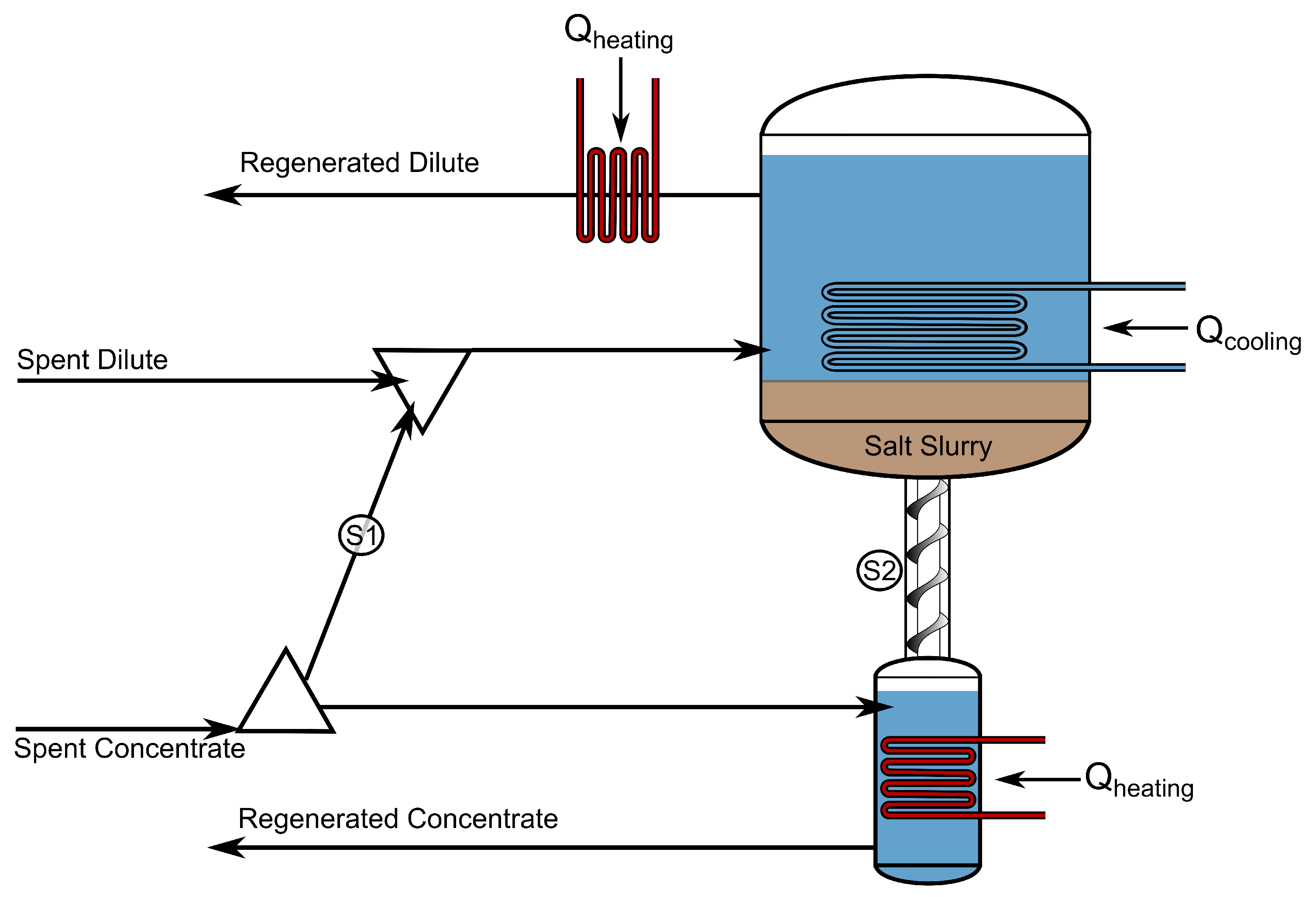
2.10. Solution Regeneration with Evaporation

A sketch of the system utilising evaporation to regenerate the electrolyte solutions is shown in Figure 2. A portion of the spent dilute, corresponding to the amount of salt that passes through the membranes, is added to the spent concentrate. This stream is led into an evaporation chamber with a vacuum circuit, where excess water is evaporated at sub-atmospheric pressure using waste heat. Evaporated water is added to the spent dilute. For the side streams denoted by subscripts $S1$ and $S2$ we have:

$$N_{e,S1}=N_{e,1}^{\mathrm{out}}-N_{e,1}^{\mathrm{in}}{N}_{w,S1}=\frac{N_{e,S1}}{m_{e,1}{M}_w}$$

(30)

$$N_{e,S2}=0N_{w,S2}=N_{w,S1}-(N_{w,1}^{\mathrm{out}}-N_{w,1}^{\mathrm{in}})$$

(31)

where the superscripts in and out refer to the variables at the inlet and outlet of the RED stack, respectively. Here, the molality of the concentrate solution exiting the distiller is fixed and equal to the initial inlet molality of the RED stack. Only the side streams necessary to return to the initial system state are calculated.

The magnitude of the salt and water side streams follows directly from the amount of these species that need to be re-introduced to the spent solutions to return to the initial state. Only the energy consumption to evaporate water is specified in the model. The evaporation enthalpy of water, ${\mathsf{\Delta }}_{vap}H$, can be used to find the amount of waste heat required to evaporate excess water from the electrolyte solution:

$$Q_{\mathrm{evap}}=N_{w,S2}{\mathsf{\Delta }}_{vap}H$$

(32)

The evaporation enthalpy dependence on solution state variables is treated in the Supplementary Materials. For electrolyte solutions at reduced pressure, the evaporation enthalpy is around 670 kWh m${}^{-3}$. However, commercial seawater thermal desalination is done with the multiple effect desalination (MED) process, in which the heat of condensation of distillate is re-used to evaporate more water in a staged process. Evaporation by these means is more energy-efficient, requiring 40–70 kWh m${}^{-3}$ of distillate [52]. Following Tamburini et al., a specific heat requirement of 40 kWh m${}^{-3}$ of distillate is adopted for the evaporation regeneration calculations [32].

2.11. Solution Regeneration with Precipitation

The precipitation concept is illustrated in Figure 3, in which the concentrate channel molality is limited to any value between the solubilities at the chosen upper and lower temperatures. The dilute channel molality is fixed by the solubility at the lower temperature. To restore the initial concentration difference between the two solutions by salt precipitation, a salt with a significant temperature dependence on the solubility is needed. The investigated salt, KCl, has a solubility of 4.15 mol kg${}^{-1}$ at a water and salt mixture temperature of 10 °C, and 5.37 mol kg${}^{-1}$ at 40 °C [53].

A portion of the spent concentrate is added to the spent dilute, this is a necessity if one is to arrive at the initial molar flow rates of both water and dissolved salt. The spent dilute is then cooled in a precipitation tank, where any salt in excess of the solubility at 10 °C precipitates. Kinetic inertia in the precipitation process is not considered here but may be an important factor. A portion of the resulting slurry in the bottom of the tank is added to the spent concentrate and the mixture is heated and dissolved, therefore bringing the concentrate back to the initial state. The upper portion of the precipitation tank contains saturated solution at 10 °C. A portion of this is extracted and heated to 40 °C, with molar flow rates equalling the initial state of the dilute channel. For the side streams denoted by subscripts $S1$ and $S2$ we have:

$$\begin{array}{cc}\hfill N_{e,S2}-N_{e,S1}& =N_{e,2}^{\mathrm{in}}-N_{e,2}^{\mathrm{out}}\hfill \\ \hfill N_{e,S2}-N_{e,S1}& =N_{e,1}^{\mathrm{out}}-N_{e,1}^{\mathrm{in}}\hfill \\ \hfill N_{w,S2}-N_{w,S1}& =N_{w,2}^{\mathrm{in}}-N_{w,2}^{\mathrm{out}}\hfill \\ \hfill N_{w,S2}-N_{w,S1}& =N_{w,1}^{\mathrm{out}}-N_{w,1}^{\mathrm{in}}\hfill \end{array}$$

(33)

which constitutes a set of four equations with the four unknowns being the molar flows of the side streams. The molar flows from the precipitation tank, $N_{e,S2}$ and $N_{w,S2}$, depend on the molality of the salt slurry in the precipitation tank.

In the precipitation concept, there are heating and cooling duties related to two processes: heating or cooling solution going out of or into the precipitation tank and precipitating or dissolving salt going into or out of the tank. Both the solution heat capacity and heat of mixing depend on composition and temperature and may be estimated using the Pitzer equations together with experimental data, as shown in the Supplementary Materials. The heating/cooling duties take the forms:

$$\begin{array}{cc}\hfill Q_1& =N_{\mathrm{tot}}{C}_p\mathsf{\Delta }T\hfill \\ \hfill Q_2& =N_e^{\mathrm{ex}}{\mathsf{\Delta }}_{\mathrm{mix}}{H}_e\hfill \end{array}$$

(34)

where $N_{\mathrm{tot}}$ is the total molar flow of solution, $C_p$ is the solution heat capacity and ${\mathsf{\Delta }}_{\mathrm{mix}}{H}_e$ is the heat of mixing per mol salt. The quantity $N_e^{\mathrm{ex}}$ is the molar flow rate of salt in excess of the solubility limit, any quantity of salt in excess of 4.15 mol kg${}^{-1}$ must be precipitated in the precipitation tank, and any solid salt extracted from the precipitation tank must be dissolved to bring the spent concentrate back to 5.37 mol kg${}^{-1}$.

Therefore, there are three important adjustable parameters for precipitation regeneration. The slurry concentration can be chosen and optimised depending on the component flows in side stream $S1$ in order to reduce the latent heat related to the precipitation and dissolving. In practice, this energy requirement is significantly smaller than the sensible heat, such that a slurry concentration of 20 mol kg${}^{-1}$ is used and optimisation is neglected. The last two parameters are the working temperature of the cell and the lower temperature in the precipitation tank, set to 40 °C and 10 °C, respectively. These two temperatures affect energy requirements in the regeneration stage, as well as conditions for the RED cell. The temperatures 40 °C and 10 °C are chosen for the first investigation using KCl.

3. Computational Procedure

Mass and energy balances for the RED stack are solved for one unit cell, and the resulting profiles of molar flows and temperature are used for the rest of the unit cells. Figure 4 illustrates the unit cell and the spatial dimensions. Membrane fluxes are in our formulation positive in the x-direction, and negative if mass or charge is transported in the opposite direction. Therefore, fluxes are positive in the x-direction in Figure 4, and then, by this logic, the subtraction of CEM fluxes in Equation (27) yields the accumulation of species in the concentrate compartment.

A total of six ordinary differential equations with membrane fluxes as source/sink terms arise from Equations (27)–(29), three for each channel in the unit cell. In the case of co-current flow in concentrate and dilute channels, this constitutes an initial value problem (IVP), with inlet molar flows and temperature as initial values. This IVP is solved in MATLAB using the differential equation solver ode15s.

The counter-current flow case has values specified at both ends of the cell, which constitutes a boundary value problem (BVP). This can be solved using a collocation method, which in MATLAB can be done using the function bvp4c. A reasonable initial estimate may be necessary for this solver to converge, and the computational mesh is chosen by the function bvp4c. The resulting profiles from the IVP are therefore used as the initial estimate for the counter-current flow case.

Solving the BVP yields the outlet state of the electrolyte solutions. Equations (30)–(32) for evaporation and Equations (33) and (34) for precipitation are then used to calculate the material streams necessary to regenerate the solutions, as well as the thermal energy required. To summarise the calculation procedure:

• The co-current flow IVP is solved using initial (inlet) values of molar flow rates of components and temperatures in one concentrate and one dilute channel. Fluxes are calculated by Equation (22) for each numerical step, and the peak power current density is used.
• The counter-current flow BVP is solved using the state variable profiles from the solved IVP as an initial guess.
• The state variable profiles from the solved BVP are used to compute the hydrogen production from the RED stack.
• The difference between the outlet and the inlet state variables is used to compute the mass and energy balances for streams $S1$ and $S2$ in order to regenerate the electrolyte solutions.

Essential parameters for the cell modelling are summarised in

Table 1. System parameters used in the REDHE modelling.

Parameter	Symbol	Value
Salt transference no. [43]	$t_s$	0.45
Water transference no. [43]	$t_w$	3
Salt diffusion coeff. [54]	$D_e$	$1\times {10}^{-12}$ m${}^2$ s${}^{-1}$
Water diffusion coeff. [54]	$D_w$	$1\times {10}^{-11}$ m${}^2$ s${}^{-1}$
IEM heat transfer coeff.	$U_m$	1000 W m${}^{-2}$K${}^{-1}$
CEM area resistance [32]	$R_{\mathrm{CEM}}$	2.96 $\mathsf{\Omega }$cm${}^2$
AEM area resistance [32]	$R_{\mathrm{AEM}}$	1.55 $\mathsf{\Omega }$cm${}^2$
IEM thickness [39]	$d_m$	125 $\mathsf{\mu }$m
IEM active area [32]	$A_m$	100 cm${}^2$
Channel length [32]	$L_{\mathrm{channel}}$	10 °Cm
Channel height [32]	$H_{\mathrm{channel}}$	10 °Cm
Channel thickness [32]	$d_{\mathrm{channel}}$	270 $\mathsf{\mu }$m
Water mass flow	$F_w$	0.27 g s${}^{-1}$
Spacer shadow factor [32]	$\beta$	1.56
Lumped overpotential [55]	$\eta$	0.2 V

. Membrane transference numbers, diffusion coefficients and resistance may vary with state variables but are here taken to be constant due to sparse data available on these properties. Other significant simplifications may be summarised as follows:

• concentration polarisation phenomena in bulk solutions are neglected;
• viscous dissipation and pressure drops are neglected;
• parasitic current draws in the feed channels of the cell are unaccounted for;
• electrode rinse solutions are assumed to have constant chemical potentials at both sides of the cell;
• variations in solution thermodynamic and transport properties with temperature are neglected; experimental data at 25 °C is used for solutions at 10 and 40 °C.

Outside of the cases where a range of concentrations or other system parameters are investigated, there are two main cases that are explored and referred to in the coming sections:

• Evaporation case: Evaporation (MED) is here used as the regeneration system. The inlet molality of concentrate is 4.5 mol kg${}^{-1}$, and 1 mol kg${}^{-1}$ for the dilute. The inlet water mass flow is 0.27 g s${}^{-1}$ and the inlet temperature is 40 °C for both channels.
• Precipitation case: Precipitation is here used as the regeneration system. The inlet molality of concentrate is 5.37 mol kg${}^{-1}$ (solubility at 40 °C), and 4.15 mol kg${}^{-1}$ (solubility at 10 °C) for the dilute. The inlet water mass flow is 0.27 g s${}^{-1}$ and the inlet temperature is 40 °C for both channels.

4. Results and Discussion

4.1. Model Validation

Relevant stack measurements of cell electric potential and resistance are, to the best of our knowledge, not available for a KCl electrolyte. Instead, the hydrogen production and power density of the RED stack predicted by the model are compared to experimental values obtained by Hatzell et al. and Chen et al. for $\mathrm{N}{\mathrm{H}}_4\mathrm{H}\mathrm{C}{\mathrm{O}}_3$ and $\mathrm{N}\mathrm{a}\mathrm{C}\mathrm{l}$ electrolytes, respectively [24,56].

The hydrogen production for a RED stack with inlet conditions specified by the evaporation case, using KCl as the electrolyte and 30 unit cells, is found to be 0.38 g${}_{{\mathrm{H}}_2}$ m${}^{-2}$h${}^{-1}$. The power density from the membrane stack (electrode overpotentials not included) is 15 W m${}^{-2}$, or on a per unit cell basis: 0.5 W m${}_{cellpair}^{-2}$. Hatzell et al. investigated hydrogen production in experiments using a 1.5 mol dm${}^{-3}$ $\mathrm{N}{\mathrm{H}}_4\mathrm{H}\mathrm{C}{\mathrm{O}}_3$ concentrate and a dilute compartment of distilled water [24]. With 20 unit cells and electrodes for the oxygen reduction reaction and hydrogen evolution reaction, the power density from the membrane stack approached 0.45 W m${}_{cellpair}^{-2}$, and the hydrogen production was roughly 0.21 g${}_{{\mathrm{H}}_2}$ m${}^{-2}$h${}^{-1}$. Chen et al. investigated hydrogen production in experiments with a concentrated $\mathrm{N}\mathrm{a}\mathrm{C}\mathrm{l}$ solution of 4 mol dm${}^{-3}$ and a dilute solution of 0.017 mol dm${}^{-3}$ [56]. With 20 unit cells, the resulting hydrogen production rate was 0.49 g${}_{{\mathrm{H}}_2}$ m${}^{-2}$h${}^{-1}$. In the future, an experimental study is necessary to determine the accuracy of the various parts of the model. However, the predicted rate of hydrogen production and the stack power density are in the expected range.

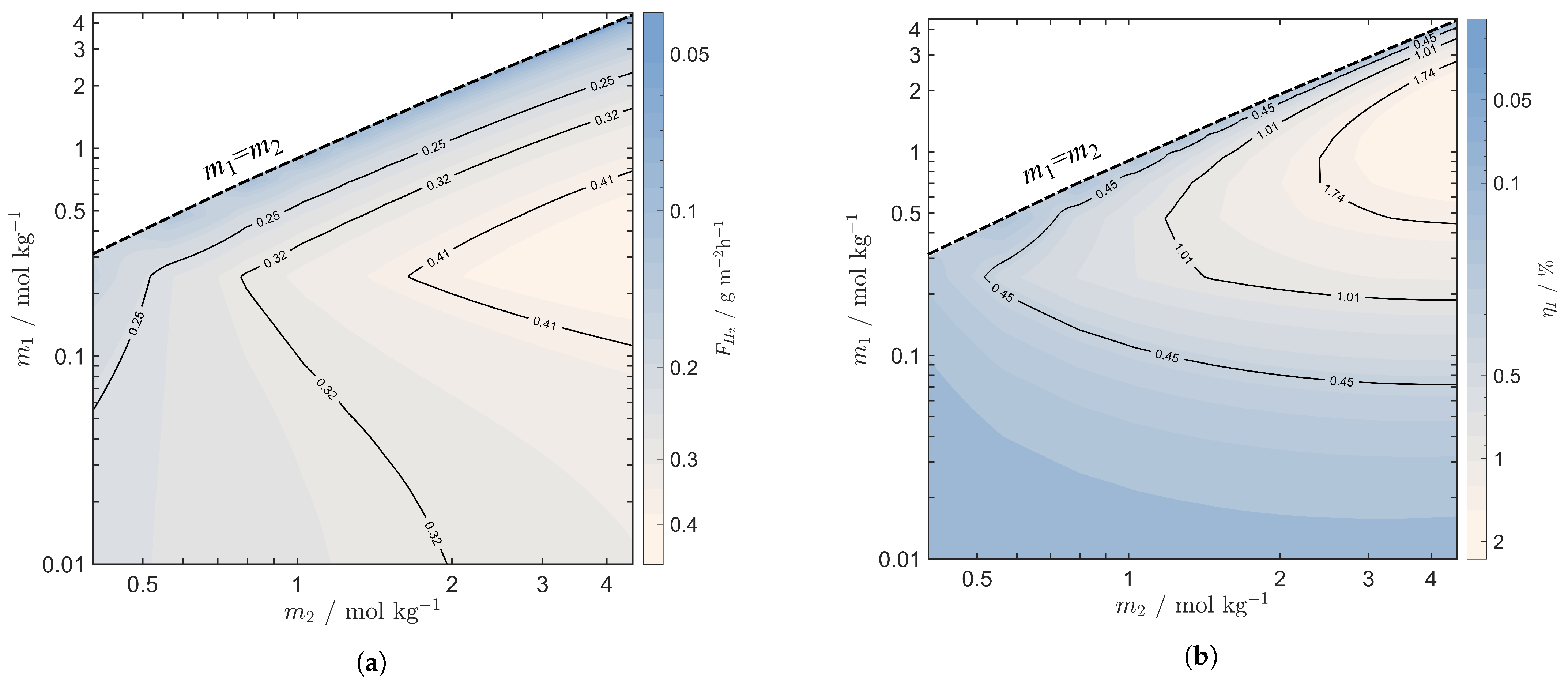
4.2. Precipitation and Evaporation Comparison

The two regeneration concepts, with stack inlet conditions specified as the evaporation case and the precipitation case, are compared using KCl as the electrolyte, where key results are shown in

Table 2. ${\mathrm{H}}_2$ production rate, total heating/cooling duties, current density, number of unit cells, and stack power calculated for the evaporation case and the precipitation case.

	Precipitation	Evaporation
$F_{H_2}$	0.14	0.38	g${}_{H_2}$ m${}^{-2}$h${}^{-1}$
$Q_{\mathrm{heating}}$	6750	1.7	kWh g${}_{H_2}^{-1}$
$j_{\mathrm{stack}}$	3.8	10	A m${}^{-2}$
$N_{\mathrm{unit}}$	286	30	-
$P_{\mathrm{stack}}$	5.4	15	W m${}^{-2}$

.

Since precipitation regeneration puts a limitation on the inlet molality of the solutions, the average voltage of the unit cells is limited as well. As a consequence, the hydrogen production and power per square meter of the active area are lower for the precipitation case than the evaporation case. Due to a low unit cell voltage, the number of unit cells required is high and a potential inhibiting factor with respect to the investment cost of the stack.

Carmo et al. reviewed hydrogen production using alkaline water electrolysis (AWE) and proton exchange membrane water electrolysis (PEMWE) [57]. The rate of production using AWE was up to 30 kg${}_{{\mathrm{H}}_2}$ m${}^{-2}$h${}^{-1}$, with an expected electricity usage of around $56\times {10}^{-2}$ kWh kg${}_{{\mathrm{H}}_2}^{-1}$. For PEMWE, a rate of up to 17 kg${}_{{\mathrm{H}}_2}$ m${}^{-2}$h${}^{-1}$ and an energy expenditure of $67\times {10}^{-2}$ kWh kg${}_{{\mathrm{H}}_2}^{-1}$ were reported. Compared to the figures presented in Table 2, the advantage of the REDHE system is not in a superior rate of hydrogen production or energy consumption, but the fact that it can use waste heat to run the system rather than electricity. Nevertheless, larger RED systems, with much larger active areas than 100 cm${}^2$, will be necessary for a competitive hydrogen production rate.

For precipitation, the heating duty presented is the sum of contributions from the heating of refreshed dilute, dissolving salt and heating the refreshed concentrate. A working temperature of 40 °C was chosen as a temperature which the membranes were likely to withstand, and 10 °C was chosen as the lower temperature to obtain a sizeable solubility difference. Other salts and operating temperatures may be relevant and may prove to be more suitable for the precipitation regeneration process due to higher solubility change with temperature. The concentrate inlet molality is not bound by the solubility at 40 °C (it is merely the upper limit) but was found to be the best case scenario for $\mathrm{K}\mathrm{C}\mathrm{l}$ solutions. The dilute molality is, however, bound by the solubility at the lower operating temperature.

The precipitation regeneration flow scheme as presented in Figure 3 was also considered by Krakhella et al. [39]. They found the thermal energy per gram of hydrogen produced required in the precipitation case to be less than for the evaporation case if the cooling required for the solution going into the precipitation tank could be used to heat the refreshed dilute. This is a non-trivial process. If the heating of the refreshed dilute stream is accounted for (and it makes up practically the whole heating demand), the thermal energy per gram of hydrogen produced is roughly 4000 times higher than for the evaporation case. The heating required per gram of hydrogen produced obtained for the evaporation case is roughly three times higher than what was found by Krakhella et al., in part due to the inclusion of electroosmotic water transference and its negative effect on the system efficiency.

The flow scheme of the precipitation regeneration system may need to be altered in order to be competitive in terms of the thermal energy requirement. Tamburini et al. investigated an $\mathrm{N}{\mathrm{H}}_4\mathrm{H}\mathrm{C}{\mathrm{O}}_3$ electrolyte which dissociates instead of precipitating, and a 4 °C change in solution temperature was necessary for the regeneration. For this dissociation case, they obtained a system efficiency of 5%, whereas, for the precipitation case presented here, the system efficiency was vanishingly small. The flow scheme they presented, with additional side flows, may reduce the amount of material flowing through the salt extraction tank. If applied to our precipitation case, it could reduce the mass flow that needs cooling and reheating.

Partial reheating of the refreshed dilute stream could also serve as an option to reduce the heating duty of the precipitation regeneration system. In such a scenario, the stream would only be heated a few degrees in order to keep salt from precipitating in the dilute channels when salt is transported through the membranes from concentrate to dilute channels. For the RED stack, this would also introduce a coupling effect between heat and mass transport across membranes. Kristiansen et al. showed that a configuration of cool dilute streams and warm concentrate streams significantly decreased the stack voltage of a seawater RED cell while reversing this temperature difference increased the stack voltage [45]. Therefore, a partial reheating of the refreshed dilute would likely be unfavourable for the performance of the stack, but beneficial in terms of reducing the required heating.

The heat exchanger area and salt precipitation in the stack are other relevant technical aspects that may inhibit the competitiveness of precipitation regeneration. Due to relatively high material flows in and out of the precipitation tank, the heating and cooling of streams may require large heat exchangers compared to the evaporation concept. With precipitation regeneration, one is also operating close to or at the solubility limits of the salt, such that crystallisation in the stack could pose a potential fouling problem.

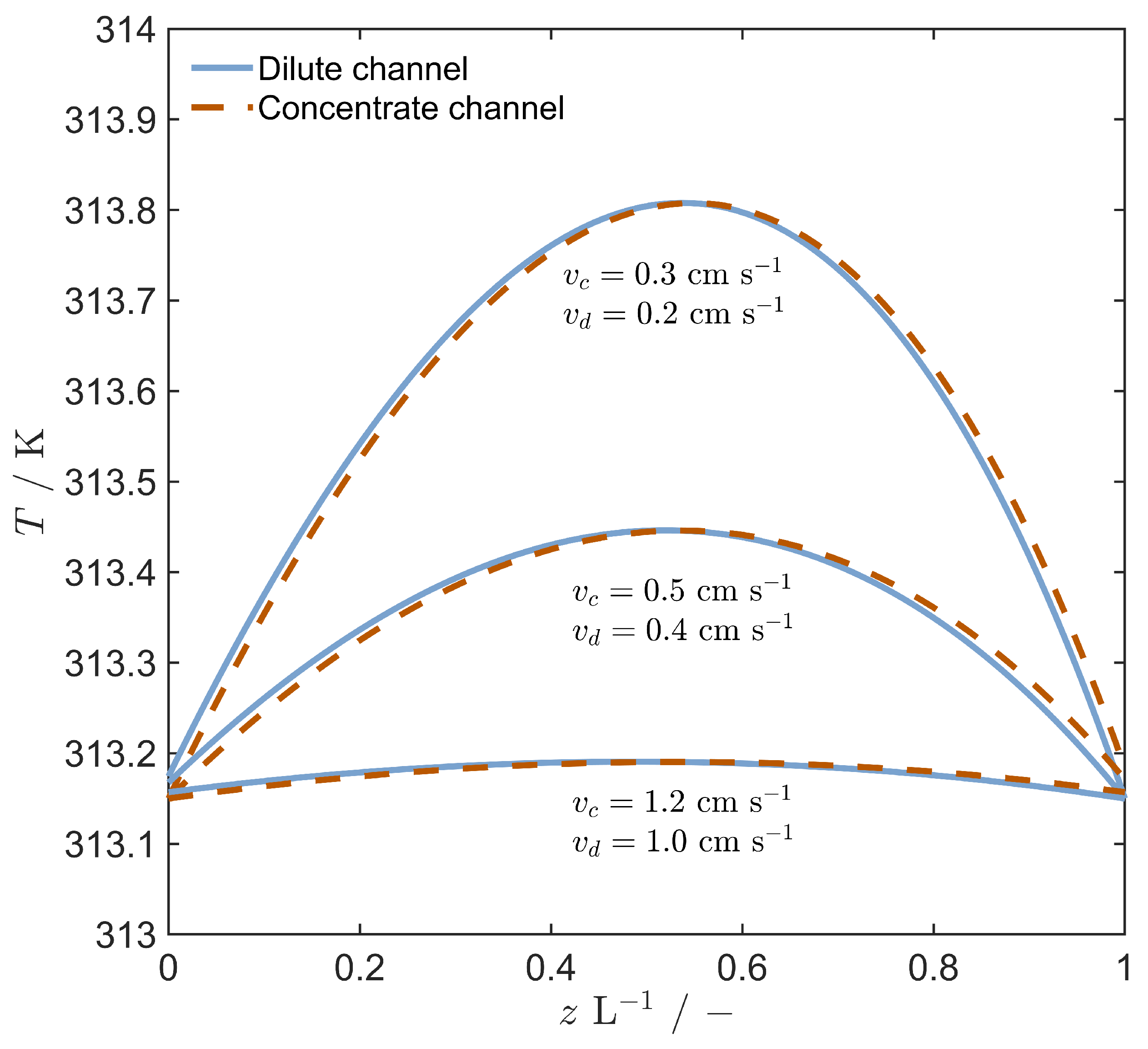
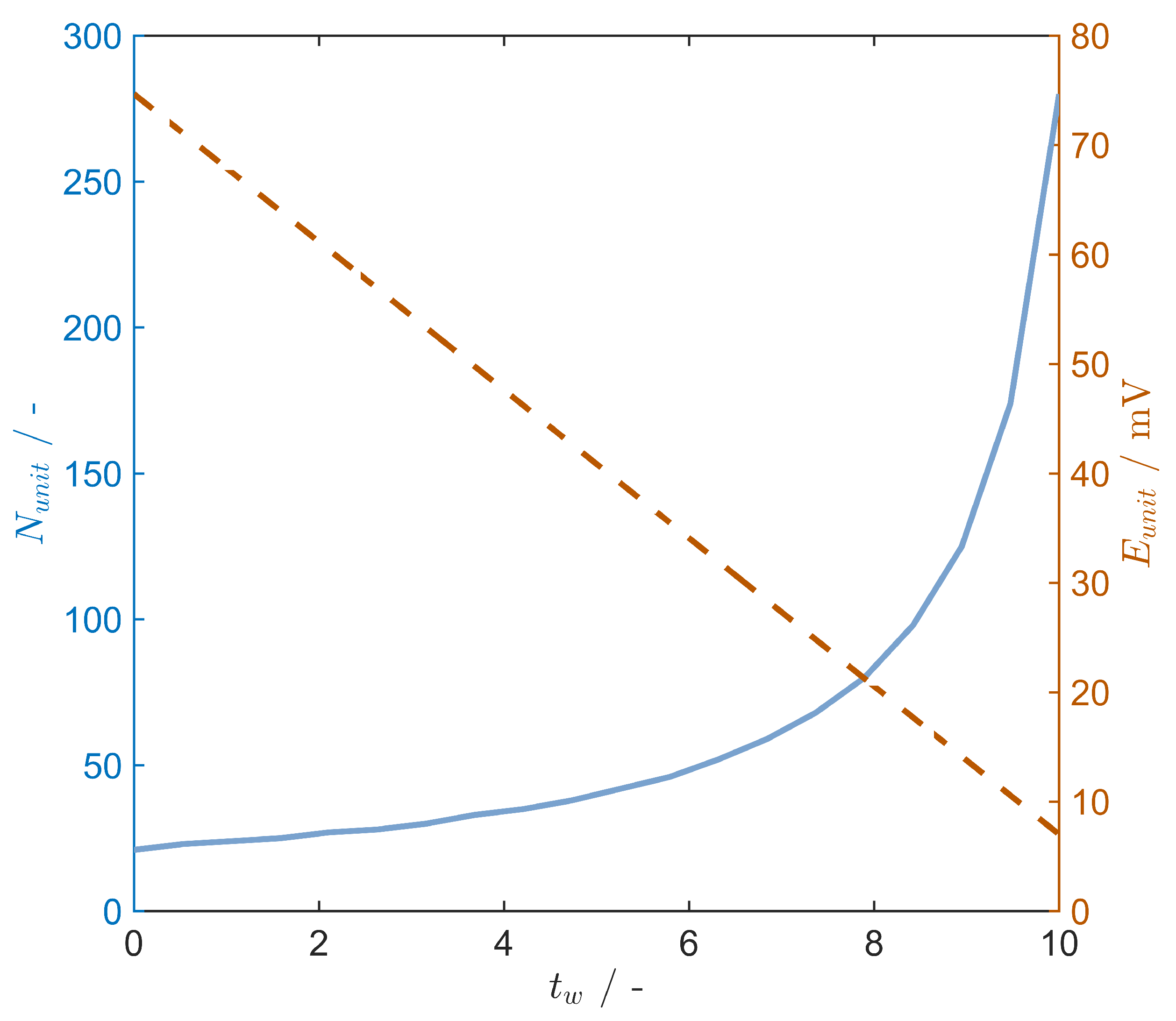
4.3. Stack Performance with Evaporation Regeneration

The results presented in Section 4.2 show that the considered concept for precipitation regeneration of electrolyte solution is not competitive with the evaporation concept, both in terms of hydrogen production and waste heat required. The remainder of this paper will therefore consider the RED stack performance with MED regeneration in further detail i.e., evaporation regeneration.

Hydrogen production and system efficiency are presented as functions of the inlet molalities of the concentrate channel, $m_2$, and the dilute channel, $m_1$, in Figure 5a,b. Generally, it is beneficial to choose a high inlet molality for the concentrate, and 0.2–1 mol kg${}^{-1}$ for the dilute channel, when the flow velocity for both channels is 1 cm s${}^{-1}$. The waste heat required to continuously regenerate the system is highly correlated with the dilute channel molality. Using a concentrate molality of 4.5 mol kg${}^{-1}$, the system efficiency decreases from 2% to 0.5% if the dilute molality is reduced from 1 mol kg${}^{-1}$ to 0.1 mol kg${}^{-1}$. The reason is that the side stream which returns salt to the spent concentrate i.e., stream $S1$ in Figure 2, also adds a significant amount of water to the spent concentrate that must be evaporated. Increasing the salt concentration in the dilute channel, therefore, decreases the amount of water that is added to the spent concentrate. Hence, the optimal dilute molality for hydrogen production is around 0.2 mol kg${}^{-1}$ due to high unit cell potential and low resistance. For the system efficiency, a dilute channel molality of 1 mol kg${}^{-1}$ is preferable. Both contour plots also feature a diagonal area where operation is inefficient, corresponding to small membrane concentration gradients. Additionally, with high salt concentrations in both channels, the influence of the water transport is at its greatest and the permselectivity is at its lowest. In terms of resistance, it is beneficial to keep both solutions above 0.1 mol kg${}^{-1}$ to obtain an acceptable electric conductivity for the electrolyte solutions.

The membrane diffusion coefficients, particularly that of salt, are also found to be important for system efficiency. Figure 6 shows the effect of varying the membrane diffusion coefficients on the evaporation unit heating duty. Larger membrane diffusion coefficients lead to a significant increase in the crossover of salt from concentrate to dilute channels, which in turn must be reintroduced into the spent concentrate along with water. If the membrane salt diffusion coefficient is increased by a factor of 10, from $D_e=1\times {10}^{-12}$ to $D_e=1\times {10}^{-11}$ m${}^2$ s${}^{-1}$, the heating duty increases from 6 W to 30 W. Consequently, the system efficiency is reduced from 2% to 0.6%. This particular result is obtained for the evaporation case with concentrate and dilute molalities of 4.5 and 1 mol kg${}^{-1}$, respectively. If the dilute channel molality is lowered, the effect of diffusion would be even more pronounced, as the driving force for diffusion would increase, in addition to the previously mentioned unwanted effect of adding more water to the spent concentrate through the side stream. To combat the effect of unwanted diffusion, the thickness of the ion-exchange membranes may be increased. The electric resistance of the membranes will also increase as a trade-off, and an optimum must be found depending on the individual ion-exchange membrane properties.

Flow velocity does not have a significant impact on the cell performance if the salt diffusion coefficient is $D_e=1\times {10}^{-12}$ m${}^2$ s${}^{-1}$, and profiles of molality, voltage and current density feature only small changes from inlet to outlet of the cell. However, concentration polarisation in channels may affect the system performance negatively at low velocities. It should be taken into account in future system assessments by using 2-dimensional mass and energy balances for the channel flows. In the case of a salt diffusion coefficient of $D_e=1\times {10}^{-11}$ m${}^2$ s${}^{-1}$, the flow velocities are more important. Then, the salt crossover is larger, such that the flow velocity, and therefore the solution residence time, has a significant impact on the molality profiles and the overall hydrogen production. The flow velocity may then be increased to reduce the variations in the molality profiles, at the cost of increasing the rate at which spent solutions must be regenerated. Once again, this trade-off must be evaluated depending on the properties of the chosen ion-exchange membranes.

The theoretical model includes the mixing enthalpy effect of components crossing the membrane and mixing with the solution on the opposite side. Temperature profiles of both channels are shown in Figure 7, indicating that the effect on the temperature is small when $D_e=1\times {10}^{-12}$ m${}^2$ s${}^{-1}$, but increases with low flow velocities. A heating effect due to the mixing takes place in both channels, and due to fast conduction between the compartments, the temperature profiles are similar. The process of dissolving $\mathrm{K}\mathrm{C}\mathrm{l}$ is endothermic, such that the heating effect taking place in the stack may be understood as net dilution of electrolyte, which is exothermic. Mass and energy balances from inlet to outlet were calculated and checked for inconsistencies.

4.4. Membrane Water Transport

The water transference number is the net amount of water transported reversibly with the electric current, in the form of hydration shells surrounding migrating ions [44]. Since the hydrated ions migrate from concentrate to dilute channels, so must the electroosmotic water flux too. Special attention is paid to the electroosmotic water transport through the membranes, as it directly affects the permselectivity through the relationship shown in Equation (14). This effect is shown in Figure 8 in terms of the unit cell potential and the required number of unit cells to drive electrolysis. With the solution concentrations specified by the evaporation case, the unit cell potential decreases around 7 mV per unit of the water transference coefficient.

The chemical potential gradient of the water is negative along the electroosmotic flux direction, and positive along the diffusion flux. One may then consider the co-transport of water as a factor that reduces the driving force for ions to migrate across the membrane [43]. For the case of a single solute in one solvent, the immediate effect is that of a lowering of permselectivity with certain combinations of molalities for the concentrate and dilute channels. The exact behaviour of the permselectivity with varying molalities, assuming that transference numbers remain fairly constant, is subject to the interaction of ions with the solvent as quantified by the activity coefficient. It is indirectly shown in Figure 5a,b, where the diagonal elements with small concentration differences have especially low permselectivity and performance. The addition of more unit cells leads to discrete steps in the total mass flow rate into and out of the stack, as well as in the rate at which solutions need to be regenerated. The effect is also present as jumps in energy consumption with increasing water transference numbers. Current density and the rate of hydrogen production decrease monotonously with increasing water transference numbers. Going from a system with perfect membranes in the evaporation case having no electroosmotic water transport, to one having $t_w=3$, the result is a 16% decrease in hydrogen production rate and a 17% increase in waste heat consumption. The system efficiency decreases from 3% to 2%. In terms of solution regeneration by evaporation, it is beneficial to minimise water crossover to the concentrate channels i.e., by diffusion, as excess water in the spent concentrate must be evaporated off. In other words, the electroosmotic water transport into the dilute reduces the heat required to regenerate to a small extent, however it does have a profound negative effect on the unit cell electric potential.

Operating the cell with inlet molalities of 4.5 mol kg${}^{-1}$ and 1 mol kg${}^{-1}$ and an active membrane area of 100 cm${}^2$ results in a power density of 15 W m${}^{-2}$ and a system efficiency of 2%. Tamburini et al. presented simulated values for a similar stack configuration with $\mathrm{N}\mathrm{a}\mathrm{C}\mathrm{l}$, but for generating electricity, which yielded power densities in the range of 70–80 W m${}^{-2}$ and a reported system efficiency of up to 5% [32]. These results indicate that other salts may be of more interest than $\mathrm{K}\mathrm{C}\mathrm{l}$. However, this was obtained with molar concentrations of 5 mol dm${}^{-3}$ and 2.2 mol dm${}^{-3}$, and constant membrane permselectivities. Since both concentrate and dilute channel molalities should be relatively high to obtain better system efficiency, the variations of the permselectivity must be taken into account, as it is especially at these high salt concentrations that the permselectivity suffers due to water transference.

5. Conclusions

A model for the reverse electrodialysis (RED) stack based on the framework of non-equilibrium thermodynamics is established, providing further insight into the membrane transport processes and their effect on the reverse electrodialysis heat engine’s (REDHE) performance. The framework of non-equilibrium thermodynamics proves helpful in understanding the complexities of the REDHE system, and in identifying key operation and material properties that need optimisation in order to efficiently produce hydrogen or electricity from waste heat. The combination of the RED model and a regeneration model points toward key parameters and their effect on the rate of hydrogen production and energy consumption, such as the membrane water transference coefficient, diffusion coefficients, and salt concentration of solutions.

Current results point to evaporation regeneration in the form of multi-effect distillation (MED) as the superior regeneration concept of those considered, both in terms of hydrogen output, waste heat required, and technical feasibility. A rethinking of the presented precipitation process is needed if it is to compete with distillation techniques such as MED. Results with $\mathrm{K}\mathrm{C}\mathrm{l}$ solutions are promising, and other solution compositions may be of interest in the future. For the evaporation regeneration case, a hydrogen production of 0.38 g${}_{{\mathrm{H}}_2}$ m${}^{-2}$h${}^{-1}$, a waste heat requirement of 1.7 kWh g${}_{{\mathrm{H}}_2}^{-1}$, and a system efficiency of 2% were obtained. The system is most efficient when both the concentrate and dilute channels have concentrations of salt above 0.5 mol kg${}^{-1}$, but at these concentrations, the water transference coefficient causes a 7 mV decrease in unit cell potential and a −0.3% decrease in system efficiency per unit of the coefficient. Additionally, using membranes with diffusion coefficients of 10${}^{-11}$ instead of 10${}^{-12}$ m${}^2$ s${}^{-1}$ could reduce the system efficiency from 2% to 0.6%, due to an increase in the amount of water that must be evaporated in the regeneration stage. These parameters must be taken into account for the optimisation of ion-exchange membranes for the REDHE concept. Future studies should aim to include concentration polarisation and composition/temperature dependency of thermodynamic and transport parameters in the model, as well as investigate new electrolyte solution compositions for increased hydrogen production rates.

References

1. Post, J.W. Blue Energy: Electricity Production from Salinity Gradients by Reverse Electrodialysis. Ph.D. Thesis, Wageningen University, Wageningen, The Netherlands, 2009. [Google Scholar]
2. Krakhella, K.W.; Morales, M.; Bock, R.; Seland, F.; Burheim, O.S.; Einarsrud, K.E. Electrodialytic Energy Storage System: Permselectivity, Stack Measurements and Life-Cycle Analysis. Energies 2020, 13, 1247. [Google Scholar] [CrossRef]
3. Scialdone, O.; Guarisco, C.; Grispo, S.; D’Angelo, A.; Galia, A. Investigation of electrode material–Redox couple systems for reverse electrodialysis processes. Part I: Iron redox couples. J. Electroanal. Chem. 2012, 681, 66–75. [Google Scholar] [CrossRef]
4. Pattle, R. Production of electric power by mixing fresh and salt water in the hydroelectric pile. Nature 1954, 174, 660. [Google Scholar] [CrossRef]
5. Loeb, S. Method and Apparatus for Generating Power Utilizing Pressure-Retarded-Osmosis. U.S. Patent 3,906,250, 19 September 1975. [Google Scholar]
6. Loeb, S. Method and Apparatus for Generating Power Utilizing Reverse Electrodialysis. U.S. Patent 4,171,409, 16 October 1979. [Google Scholar]
7. Tedesco, M.; Scalici, C.; Vaccari, D.; Cipollina, A.; Tamburini, A.; Micale, G. Performance of the first reverse electrodialysis pilot plant for power production from saline waters and concentrated brines. J. Membr. Sci. 2016, 500, 33–45. [Google Scholar] [CrossRef]
8. Papapetrou, M. Reverse Electrodialysis Power Production-Progress in the development of an innovative system. In Proceedings of the 4th International Conference on Ocean Energy, Dublin, Ireland, 17 October 2012. [Google Scholar]
9. Tedesco, M.; Cipollina, A.; Tamburini, A.; van Baak, W.; Micale, G. Modelling the Reverse ElectroDialysis process with seawater and concentrated brines. Desalin. Water Treat. 2012, 49, 404–424. [Google Scholar] [CrossRef]
10. Tedesco, M.; Cipollina, A.; Tamburini, A.; Micale, G.; Helsen, J.; Papapetrou, M. REAPower: Use of desalination brine for power production through reverse electrodialysis. Desalin. Water Treat. 2015, 53, 3161–3169. [Google Scholar] [CrossRef]
11. Tufa, R.A.; Curcio, E.; van Baak, W.; Veerman, J.; Grasman, S.; Fontananova, E.; Di Profio, G. Potential of brackish water and brine for energy generation by salinity gradient power-reverse electrodialysis (SGP-RE). RSC Adv. 2014, 4, 42617–42623. [Google Scholar] [CrossRef]
12. Tedesco, M.; Brauns, E.; Cipollina, A.; Micale, G.; Modica, P.; Russo, G.; Helsen, J. Reverse electrodialysis with saline waters and concentrated brines: A laboratory investigation towards technology scale-up. J. Membr. Sci. 2015, 492, 9–20. [Google Scholar] [CrossRef]
13. Tedesco, M.; Cipollina, A.; Tamburini, A.; Micale, G. Towards 1 kW power production in a reverse electrodialysis pilot plant with saline waters and concentrated brines. J. Membr. Sci. 2017, 522, 226–236. [Google Scholar] [CrossRef]
14. Ni, M.; Leung, M.K.; Leung, D.Y. Energy and exergy analysis of hydrogen production vby a proton exchange membrane (PEM) electrolyzer plant. Energy Convers. Manag. 2008, 49, 2748–2756. [Google Scholar] [CrossRef]
15. Kumar, S.S.; Himabindu, V. Hydrogen production by PEM water electrolysis–A review. Mater. Sci. Energy Technol. 2019, 2, 442–454. [Google Scholar]
16. Lamb, J.J.; Burheim, O.S.; Pollet, B.G. Hydrogen Fuel Cells and Water Electrolysers. In Micro-Optics and Energy; Springer Nature Switzerland AG: Cham, Switzerland, 2020; pp. 61–71. [Google Scholar]
17. Lamb, J.J.; Hillestad, M.; Rytter, E.; Bock, R.; Nordgård, A.S.; Lien, K.M.; Burheim, O.S.; Pollet, B.G. Traditional routes for hydrogen production and carbon conversion. In Hydrogen, Biomass and Bioenergy: Integration Pathways for Renewable Energy Applications; Academic Press: Cambridge, MA, USA, 2020; p. 21. [Google Scholar]
18. Lamb, J.J.; Pollet, B.G.; Burheim, O.S. Energy storage. In Energy-Smart Buildings Design: Construction and Monitoring of Buildings for Improved Energy Efficiency; IOP Publishing: Bristol, UK, 2020. [Google Scholar] [CrossRef]
19. Rytter, E.; Hillestad, M.; Austbø, B. Thermochemical production of fuels. In Hydrogen, Biomass and Bioenergy: Integration Pathways for Renewable Energy Applications; Academic Press: Cambridge, MA, USA, 2020; p. 89. [Google Scholar]
20. Borgschulte, A. The hydrogen grand challenge. Front. Energy Res. 2016, 4, 11. [Google Scholar] [CrossRef]
21. Boyano, A.; Blanco-Marigorta, A.; Morosuk, T.; Tsatsaronis, G. Exergoenvironmental analysis of a steam methane reforming process for hydrogen production. Energy 2011, 36, 2202–2214. [Google Scholar] [CrossRef]
22. Rand, D.A. A journey on the electrochemical road to sustainability. J. Solid State Electrochem. 2011, 15, 1579–1622. [Google Scholar] [CrossRef]
23. Acar, C.; Dincer, I. Comparative assessment of hydrogen production methods from renewable and non-renewable sources. Int. J. Hydrog. Energy 2014, 39, 1–12. [Google Scholar] [CrossRef]
24. Hatzell, M.C.; Ivanov, I.; Cusick, R.D.; Zhu, X.; Logan, B.E. Comparison of hydrogen production and electrical power generation for energy capture in closed-loop ammonium bicarbonate reverse electrodialysis systems. Phys. Chem. Chem. Phys. 2014, 16, 1632–1638. [Google Scholar] [CrossRef]
25. Tamburini, A.; Cipollina, A.; Papapetrou, M.; Piacentino, A.; Micale, G. Salinity gradient engines. In Sustainable Energy from Salinity Gradients; Woodhead Publishing: Sawston, UK, 2016; pp. 219–256. [Google Scholar]
26. Johnson, I.; Choate, W.T.; Davidson, A. Waste Heat Recovery. Technology and Opportunities in U.S. Industry; Technical Report; U.S. Department of Energy: Washington, DC, USA, 2008. [Google Scholar] [CrossRef]
27. Miró, L.; Brückner, S.; Cabeza, L.F. Mapping and discussing Industrial Waste Heat (IWH) potentials for different countries. Renew. Sustain. Energy Rev. 2015, 51, 847–855. [Google Scholar] [CrossRef]
28. Hammond, G.; Norman, J. Heat recovery opportunities in UK industry. Appl. Energy 2014, 116, 387–397. [Google Scholar] [CrossRef]
29. Papapetrou, M.; Kosmadakis, G.; Cipollina, A.; La Commare, U.; Micale, G. Industrial waste heat: Estimation of the technically available resource in the EU per industrial sector, temperature level and country. Appl. Therm. Eng. 2018, 138, 207–216. [Google Scholar] [CrossRef]
30. Rattner, A.S.; Garimella, S. Energy harvesting, reuse and upgrade to reduce primary energy usage in the USA. Energy 2011, 36, 6172–6183. [Google Scholar] [CrossRef]
31. Horenburg, P. Transforming Waste Heat into Electricity. Steam Expansion Engine Makes Efficient and Flexible Use of Low-Temperature Heat with ORC Technology; Bundesministerium fuer Wirtschaft und Technologie (BMWi): Berlin, Germany, 2011. [Google Scholar]
32. Tamburini, A.; Tedesco, M.; Cipollina, A.; Micale, G.; Ciofalo, M.; Papapetrou, M.; Van Baak, W.; Piacentino, A. Reverse electrodialysis heat engine for sustainable power production. Appl. Energy 2017, 206, 1334–1353. [Google Scholar] [CrossRef]
33. Zimmermann, P.; Solberg, S.B.B.; Tekinalp, Ö.; Lamb, J.J.; Wilhelmsen, Ø.; Deng, L.; Burheim, O.S. Heat to Hydrogen by RED—Reviewing Membranes and Salts for the RED Heat Engine Concept. Membranes 2022, 12, 48. [Google Scholar] [CrossRef] [PubMed]
34. Ortega-Delgado, B.; Giacalone, F.; Catrini, P.; Cipollina, A.; Piacentino, A.; Tamburini, A.; Micale, G. Reverse electrodialysis heat engine with multi-effect distillation: Exergy analysis and perspectives. Energy Convers. Manag. 2019, 194, 140–159. [Google Scholar] [CrossRef]
35. Kim, D.H.; Park, B.H.; Kwon, K.; Li, L.; Kim, D. Modeling of power generation with thermolytic reverse electrodialysis for low-grade waste heat recovery. Appl. Energy 2017, 189, 201–210. [Google Scholar] [CrossRef]
36. Olkis, C.; Brandani, S.; Santori, G. Adsorption reverse electrodialysis driven by power plant waste heat to generate electricity and provide cooling. Int. J. Energy Res. 2021, 45, 1971–1987. [Google Scholar] [CrossRef]
37. Bevacqua, M.; Tamburini, A.; Papapetrou, M.; Cipollina, A.; Micale, G.; Piacentino, A. Reverse electrodialysis with NH4HCO3-water systems for heat-to-power conversion. Energy 2017, 137, 1293–1307. [Google Scholar] [CrossRef]
38. Papapetrou, M.; Kosmadakis, G.; Giacalone, F.; Ortega-Delgado, B.; Cipollina, A.; Tamburini, A.; Micale, G. Evaluation of the Economic and Environmental Performance of Low-Temperature Heat to Power Conversion using a Reverse Electrodialysis—Multi-Effect Distillation System. Energies 2019, 12, 3206. [Google Scholar] [CrossRef]
39. Krakhella, K.W.; Bock, R.; Burheim, O.S.; Seland, F.; Einarsrud, K.E. Heat to H2: Using waste heat for hydrogen production through reverse electrodialysis. Energies 2019, 12, 3428. [Google Scholar] [CrossRef]
40. Raka, Y.D.; Karoliussen, H.; Lien, K.M.; Burheim, O.S. Opportunities and challenges for thermally driven hydrogen production using reverse electrodialysis system. Int. J. Hydrog. Energy 2020, 45, 1212–1225. [Google Scholar] [CrossRef]
41. Raka, Y.D.; Bock, R.; Karoliussen, H.; Wilhelmsen, Ø.; Burheim, O.S. The Influence of Concentration and Temperature on the Membrane Resistance of Ion Exchange Membranes and the Levelised Cost of Hydrogen from Reverse Electrodialysis with Ammonium Bicarbonate. Membranes 2021, 11, 135. [Google Scholar] [CrossRef]
42. Wu, X.; Gong, Y.; Xu, S.; Yan, Z.; Zhang, X.; Yang, S. Electrical Conductivity of Lithium Chloride, Lithium Bromide, and Lithium Iodide Electrolytes in Methanol, Water, and Their Binary Mixtures. J. Chem. Eng. Data 2019, 64, 4319–4329. [Google Scholar] [CrossRef]
43. Zlotorowicz, A.; Strand, R.V.; Burheim, O.S.; Wilhelmsen, Ø.; Kjelstrup, S. The permselectivity and water transference number of ion exchange membranes in reverse electrodialysis. J. Membr. Sci. 2017, 523, 402–408. [Google Scholar] [CrossRef]
44. Signe Kjelstrup, D.B. Non-Equilibrium Thermodynamics of Heterogeneous Systems; World Scientific: Singapore, 2008. [Google Scholar]
45. Kristiansen, K.R.; Barragán, V.M.; Kjelstrup, S. Thermoelectric Power of Ion Exchange Membrane Cells Relevant to Reverse Electrodialysis Plants. Phys. Rev. Appl. 2019, 11, 044037. [Google Scholar] [CrossRef]
46. Førland, T.F.K.S.; Kjelstrup, S. Irreversible Thermodynamics: Theory and Applications; Wiley: Chichester, UK, 1988. [Google Scholar]
47. Bedeaux, D.; Kjelstrup, S. Local Properties of a Formation Cell as Described by Nonequilibrium Thermodynamics. J. Non-Equilib. Thermodyn. 2000, 25, 161–178. [Google Scholar] [CrossRef]
48. Friedman, H.L. Thermodynamic Excess Functions for Electrolyte Solutions. J. Chem. Phys. 1960, 32, 1351–1362. [Google Scholar] [CrossRef]
49. Zhang, W.; Chen, X.; Wang, Y.; Wu, L.; Hu, Y. Experimental and Modeling of Conductivity for Electrolyte Solution Systems. ACS Omega 2020, 5, 22465–22474. [Google Scholar] [CrossRef]
50. Jakobsen, H.A. Chemical Reactor Modeling; Springer: New York, NY, USA, 2014. [Google Scholar]
51. Wilhelmsen, Ø.; Anantharaman, R.; Berstad, D.; Jordal, K. Multi-Scale modelling of a membrane reforming power cycle with CO2 capture. In 21st European Symposium on Computer Aided Process Engineering; Computer Aided Chemical Engineering; Pistikopoulos, E., Georgiadis, M., Kokossis, A., Eds.; Elsevier: Amsterdam, The Netherlands, 2011; Volume 29, pp. 6–10. [Google Scholar] [CrossRef]
52. Micale, G.; Cipollina, A.; Rizzuti, L. Seawater Desalination for Freshwater Production. In Seawater Desalination: Conventional and Renewable Energy Processes; Springer: Berlin/Heidelberg, Germany, 2009; Chapter 1; pp. 1–15. [Google Scholar] [CrossRef]
53. Rumble, J.R. Aqueous solubility of inorganic compounds at various tempratures. In CRC Handbook of Chemistry and Physics, 101st ed.; CRC Press/Taylor & Francis: Boca Raton, FL, USA, 2020. [Google Scholar]
54. Veerman, J.; de Jong, R.M.; Saakes, M.; Metz, S.J.; Harmsen, G.J. Reverse electrodialysis: Comparison of six commercial membrane pairs on the thermodynamic efficiency and power density. J. Membr. Sci. 2009, 343, 7–15. [Google Scholar] [CrossRef]
55. Burheim, O.S. Engineering Energy Storage; Elsevier: Amsterdam, The Netherlands, 2017. [Google Scholar]
56. Chen, X.; Jiang, C.; Zhang, Y.; Wang, Y.; Xu, T. Storable hydrogen production by Reverse Electro-Electrodialysis (REED). J. Membr. Sci. 2017, 544, 397–405. [Google Scholar] [CrossRef]
57. Carmo, M.; Fritz, D.L.; Mergel, J.; Stolten, D. A comprehensive review on PEM water electrolysis. Int. J. Hydrogen Energy 2013, 38, 4901–4934. [Google Scholar] [CrossRef]
58. Pitzer, K.S.; Mayorga, G. Thermodynammics of Electrolytes. II. Activity and Osmotic Coefficients for Strong Electrolytes with One or Both Ions Univalent. J. Phys. Chem. 1973, 77, 134–140. [Google Scholar] [CrossRef]
59. Saluja, P.P.S.; Pitzer, K.S.; Phutela, R.C. High-temperature thermodynamic properties of several 1:1 electrolytes. Can. J. Chem. 1986, 64, 1278–1285. [Google Scholar] [CrossRef]
60. Stokes, R.H.; Robinson, R.A. Ionic hydration and activity in electrolyte solutions. J. Am. Chem. Soc. 1948, 70, 1870–1878. [Google Scholar] [CrossRef]
61. Lobo, V.M.M.; Quaresma, J.L. Handbook of Electrolyte Solutions, Part A; Elsevier: Amsterdam, The Netherlands, 1989. [Google Scholar]
62. Lobo, V.M.M.; Quaresma, J.L. Handbook of Electrolyte Solutions, Part B; Elsevier: Amsterdam, The Netherlands, 1989. [Google Scholar]
63. Dobos, D. Electrochemical Data; Elsevier: Amsterdam, The Netherlands, 1975. [Google Scholar]
64. Clarke, E.C.W.; Glew, D.N. Evaluation of Debye–Hückel limiting slopes for water between 0 and 150 °C. J. Chem. Soc. Faraday Trans. 1980, 76, 1911–1916. [Google Scholar] [CrossRef]
65. Silvester, L.F.; Pitzer, K.S. Thermodynamics of electrolytes. X. Enthalpy and the effect of temperature on the activity coefficients. J. Solut. Chem. 1978, 7, 327–337. [Google Scholar] [CrossRef]
66. Chase, M. NIST-JANAF Thermochemical Tables, 4th ed.; American Institute of Physics: College Park, MD, USA, 1998. [Google Scholar]
67. Ge, X.; Wang, X. Estimation of Freezing Point Depression, Boiling Point Elevation, and Vaporization Enthalpies of Electrolyte Solutions. Ind. Eng. Chem. Res. 2009, 48, 2229–2235. [Google Scholar] [CrossRef]
68. Criss, C.M.; Millero, F.J. Modeling the Heat Capacities of Aqueous 1-1 Electrolyte Solutions with Pitzer’s Equations. J. Phys. Chem 1996, 100, 1288–1294. [Google Scholar] [CrossRef]
Figure 1. The RED stack showing local flux directions of cations (M+) and anions (X) through the cation-exchange membranes (CEMs) and anion-exchange membranes (AEMs). Concentrate (2) and dilute solutions (1) flow in counter-current directions, and electrode compartments at each end of the stack are filled with a circulating rinse solution (r). The smallest repeating pattern of solutions and membranes is referred to as a unit cell.
Energies 15 06011 g001
Figure 2. Conceptual sketch of the evaporation regeneration stage with spent dilute and concentrate coming from the outlet of the RED stack. Pumps required for solution propulsion are not shown, only pumps related to the vacuum circuit. All salt that passes the membranes to the dilute side of the RED stack is returned to the concentrate side through S 1 , bringing some water along. Any excess water on the concentrate side is evaporated and added to the dilute side through S 2 .
Energies 15 06011 g002
Figure 3. Conceptual sketch of the precipitation regeneration stage with spent dilute and concentrate coming from the outlet of the RED stack. Pumps required for solution propulsion are not shown. Water and salt are exchanged between spent concentrate and dilute through S 1 and S 2 , in amounts depending on the slurry concentration and the state of the spent solutions.
Energies 15 06011 g003
Figure 4. Sketch of the computational domain of the unit cell plus one additional CEM. Flux arrows show the positive direction, which may not correspond to the actual direction of transport.
Energies 15 06011 g004
Figure 5. Contour plots of simulated (a) hydrogen production, F H 2 , and (b) system efficiency, η I , as function of the inlet molalities of the concentrate channel, m 2 , and of the dilute channel, m 1 , for the evaporation case, and m 1 > m 2 is not shown.
Energies 15 06011 g005
Figure 6. Required heating duty, Q h e a t i n g , for the evaporation case as function of the diffusion coefficients. The salt diffusion coefficient is varied with a constant water diffusion coefficient of D w = 1 × 10 11 m 2 s 1 (dashed line, orange), and the water diffusion coefficient is varied with a constant salt diffusion coefficient of D e = 1 × 10 12 m 2 s 1 (solid line, blue).
Energies 15 06011 g006
Figure 7. Temperature profiles of concentrate (dashed line, orange) and dilute (solid line, blue) channels with varied flow velocities. Inlet temperature and salt molalities are specified by the evaporation case. Dilute flow enters the cell at z L 1 = 1 , concentrate enters at z L 1 = 0 .
Energies 15 06011 g007
Figure 8. Number of unit cells required for electrolysis (solid line, blue) and unit cell potential (dashed line, orange) as a function of the water transference number for the evaporation case.
Energies 15 06011 g008