
A Finite-Time Differentiator with Application to Nuclear Reactor Inverse Period Measurement


Key Laboratory of Advanced Reactor Engineering and Safety of Ministry of Education, Collaborative Innovation Centre of Advanced Nuclear Energy Technology, Institute of Nuclear and New Energy Technology, Tsinghua University, Beijing 100084, China
*
Authors to whom correspondence should be addressed.
Energies 2022, 15(12), 4487; https://doi.org/10.3390/en15124487
Submission received: 27 May 2022
/
Revised: 15 June 2022
/
Accepted: 17 June 2022
/
Published: 20 June 2022
(This article belongs to the Special Issue Nuclear Power Instrumentation and Control)
Abstract
:The measurement of the growth rate, or the so-called inverse period, of a nuclear reactor is crucial for safety monitoring and control purposes. Due to the inevitable statistical fluctuation of neutron flux at low power-levels, it is difficult to precisely estimate the inverse period from the pulse counting data in the source range. Motivated by the equivalence of the measurement of inverse period and the differentiation of the logarithm of pulse count, a new differentiator is proposed, which is finite-time convergent with a bounded steady estimation error. The feasibility of this newly-built finite-time differentiator is verified by numerical simulation. Then, based on the pulse count data recorded during the startup of a test reactor, the differentiator is used to estimate the inverse period and its derivative, as well as the period and the reactivity of the reactor. The results show that the differentiator is capable of providing a satisfactory estimation of signal derivatives under strong noise.
1. Introduction
The period of a nuclear reactor is defined as the e-folding time of neutron flux. In nuclear engineering, the reactor period is an important parameter, which is taken to be positive for a flux increase and negative for a flux decrease [1]. The reciprocal of the reactor period, also called the growth rate or the inverse period, shows the fractional increase in the neutron flux per second, i.e.,
where n(t) is the neutron flux of a nuclear fission reactor, and ω denotes the inverse period. Reactor period T can be given as
The measurement of the period or inverse period is needed for reactor control and safety purposes [2,3]. For example, the worth of a control rod can be calibrated through measuring the period related to an incremental withdrawal of the rod [3]. At low power-levels, such measurement is normally performed in the pulse channel, where each electrical impulse represents the detection of an individual neutron. Hence, neutron flux n(t) is measured by the pulse count per second in the pulse channel. However, due to the inherent statistical fluctuation of neutron flux at low power-levels, it is difficult to accurately measure the inverse period by directly differentiating the signal given by the logarithm of pulse count based on the traditional numerical difference method [4].
Actually, the necessity of estimating the time-derivative of signals arises in many areas of system monitoring and control, such as target tracking and motion analysis. The derivative of a signal can be approximated by its numerical difference roughly, and can also be estimated based upon a differentiator precisely. Here, a differentiator is a special state-observer providing both the estimates of several orders of the derivatives and the reconstruction of the original signal. In the past almost three decades, some promising results of differentiator design have been given, which can be classified into linear and nonlinear differentiators. The idea of linear differentiator design is to approximate the transfer function of an ideal differentiator while filtering out the noises. Khalil gave the linear high-gain observer (HGO) which can be able to provide the estimates of the time-derivatives of a signal up to (n − 1)th order, where n is the dimension of the state-vector of HGO [5,6]. To avoid the peaking phenomenon induced by high gains, Ibrir proposed a Kalman filter-like linear differentiator, whose time-varying gain matrix is given by the solution of a differential Riccati equation [7,8]. To further enhance the convergence, the development of nonlinear differentiators is then concerned. Based on the sliding mode technique, Levant proposed a first-order [9] as well as a high-order [10] differentiator. Although these sliding mode differentiators are finite-time convergent, the main drawback is the chattering phenomenon induced by the sign function. Motivated by the bang-bang control of integrator chains, Han et al. proposed the tracking differentiator (TD) [11]. It is shown by the comparison study [12] that the TD has a weaker stability requirement of the original systems utilized for differentiator design than those linear differentiators presented in [5,6,7,8] do. The rigorous convergence analysis of TD can be found in [13,14]. Further, a finite-time-convergent differentiator is proposed in [15] based on the perturbation technique as well as some well-constructed finite-time stable systems. The construction of finite-time stable systems can be realized by designing finite-time stabilizers for an integrator chain [16,17]. By designing a new finite-time stabilizer of the 2nd-order integrator chain, a 1st-order differentiator is newly given in [18]. However, since the expressions of the finite-time stabilizers of integrator chains presented in [16,17,18] are complicated, the corresponding differentiators cannot be easily implemented in practical engineering, which lead to the need for developing simple and effective differentiators.
It can be seen from (1) that the inverse period is essentially the derivative of signal v defined by v(t) = lnn(t). Motivated by the equivalence of the measurement of the inverse period and the differentiation of signal v, a simple nonlinear differentiator is first proposed, which is finite-time convergent with a bounded steady estimation error. Then, the feasibility of the newly-built differentiator is verified through numerical simulation. Finally, the differentiator is applied to estimate the inverse period and its derivative as well as the period and the reactivity of a test reactor from the pulse counting data recorded during the reactor startup.
2. Introduction to Homogeneity and Finite-Time Stability
In this section, the concepts about homogeneity and finite-time stability are first introduced. Then, both the lemma giving the sufficient condition of finite-time stability and that showing the properties of homogeneous systems are given.
Definition 1 (δr-Homogeneity).
Fix a set of coordinates x = [x1, …, xn]T in Rn. Let r = (r1, …, rn) be a n-tuple of positive real numbers. Then, the definitions of the one-parameter dilation, homogeneous function and homogeneous vector are given as follows:
- (1)
- The one-parameter dilation associated with r is defined bywhere ε > 0, = [x1, …, xn]T∈Rn, and the numbers ri (i = 1, …, n) are the weights of coordinates.
- (2)
- A function V: Rn→R is said to be δr-homogenous of degree m (m∈R) if
- (3)
- A vector function f(x) = [f1(x), …, fn(x)]T is said to be δr-homogenous of degree k (k∈R) if fi(x) is δr-homogenous of degree k + ri (i = 1, …, n), i.e.,
Definition 2 (δr-homogeneous norm [19]).
Let r = (r1, …, rn) be a n-uplet of positive real numbers. For∀x = [x1, …, xn]T∈Rn, a δr-homogeneous norm is given by
where p ≥ 1. Moreover, the set given by
is the corresponding δr-homogeneous unit sphere.
Definition 3 (Finite-Time Stability).
Consider the following nonlinear system
where f: D→Rn is continuous, O∈D, and f(O) = O. The equilibrium x = O is finite-time stable if it is Lyapunov stable and there exits a function T: D/{O}→(t0,∞) such that, for any x0∈ U/{O}, system trajectory x(t) with x(t0) = x0 satisfies
where t∈[t0,T(x0)), and T(x0) is called the settling time. Further, if D = Rn, then the origin is globally finite-time stable.
Lemma 1.
Consider nonlinear system (4). If there exists a real scalar γ∈ (0,1), a positive scalar c and a continuously differentiable Lyapunov function V(x) so that inequality holds along the trajectories starting at any initial point x0, then the origin is a finite-time stable, and the settling time satisfies
Lemma 2.
where RA is the attraction region of the origin.
Consider nonlinear system (4), and suppose that system vector f is δr-homogenous of degree h, where h∈R. If the origin x = O is asymptotically stable, then it can be seen that
- (1)
- For∀d > 0, there exists a Lyapunov function V that is δr- homogenous of degree d.
- (2)
- If h < 0, then the origin is finite-time stable.
- (3)
- There exists positive constants Bi (i = 1, …, n) so that
Proof.
The detailed proof is given in the Appendix A. □
3. Finite-Time Differentiator Design
In this section, a simple nonlinear differentiator is proposed, and it is shown by theoretical analysis that this differentiator is finite-time convergent with a bounded steady error. Based upon Lemma 2, the following Theorem 1 gives a finite-time stable original system for differentiator design, which is the first main result of this paper.
Theorem 1.
Consider dynamic system
where xi∈ R are the state-variables, ki are positive constants,
i = 1, …, n, sgn(∙) is the sign function given by
and α is a given constant satisfying
System (6) is finite-time stable around the origin x = O if the algebraic equation
where s∈ C, is Hurwitz, i.e., all the roots have strictly negative real parts.
Proof.
First, we show that system (6) is asymptotically stable around the origin.
Define
Then, the linearized system corresponding to system (6) at xe can be written as
where
and
From (15), the characteristic equation corresponding to system matrix A(ρ) is given by
where p ∈ C. Define
and (17) can be rewritten as (12). Since Equation (12) is Hurwitz, system (6) is asymptotically stable around xe that can be arbitrarily close to the origin by setting constant ρ to be small enough.
Suppose that system (6) is not asymptotically stable at the origin, which means that there exists a positive constant M > 0 so that
From (13), it can be seen the fact
which means that ‖xe(ρ)‖ < M/2 if positive constant ρ is small enough. Since (6) is asymptotically stable around xe(ρ), there exists T > 0 so that
which further gives
Because of the contradiction between inequalities (19) and (20), system (6) must be asymptotically stable at the origin.
Second, we show the homogeneity property of system vector f(x) given by
Actually, it can be seen by direct calculation that
Then, from Definition 1 and Equation (22), system vector f(x) is δr-homogenous of degree α − 1. It can be further seen from (11) that −1/n < α − 1 < 0.
Since system (6) is asymptotically stable at the origin, and system vector f(x) is δr-homogenous with a negative degree, it can be seen from Lemma 2 that system (6) is finite-time stable at the origin, which completes the proof of Theorem 1. □
Remark 1.
As α → 1, system (6) converges to system
where
The trajectory of system (23) is given by
where x0 is the initial point. Since the characteristic equation of matrix Ac is just (12) which is Hurwitz, i.e., all the eigenvalues of Ac have negative real parts. Then, from (25), system (23) is exponentially stable at the origin x = O. Hence, positive constant α cannot equal to 1, otherwise the finite-time stability of the origin will degrade to the asymptotic stability.
Based on the system given by (6)–(11), design the (n − 1)th-order differentiator of signal v(t) as
where ε > 0 is an arbitrarily given positive constant, θi is given by (8), i = 1, …, n. It can be seen that differentiator (26) not only gives the derivatives of signal v(t) up to (n − 1)th order but also provides the reconstruction of v(t) from noises. The following Theorem 2, which is the second main result, shows finite-time convergence of differentiator (26).
Theorem 2.
Differentiator (26) is finite-time convergent with a bounded steady error if the associated system given by (6)–(11) is finite-time stable.
Proof.
Define the time-scale transformation as
and define the coordinate transformation as
where v(i) is the ith order derivative of signal v(t).
From scale transformation (27) and coordinate transformation (28), (n − 1)th-order differentiator (26), where integer n should be larger than 2, can be rewritten as
where
In practical engineering, both signal v(t) and its derivatives are bounded in most cases, and hence it is not loss of generality to assume that scalar Δ given by (30) is bounded, i.e., there exists a positive constant M so that
From Lemma 2, for an arbitrarily given positive constant d, there exits a Lyapunov function V that is δr-homogenous of degree d while satisfying
where h = α − 1 < 0, and α is the positive constant limited by (11). Then, from the proof of Lemma 2 given in the Appendix A, it can be derived that
From inequality (34), we can see that
where RA is the domain of attraction of the origin x = O, and
Based upon (35) and (36), the state-vector x converges to bounded set Ξ in finite-time. Further, it can be seen from (28) that state-variables xi (i = 1, …, n) is the estimation error of signal v(t) and its derivatives up to the (n − 1)th order. Hence, differentiator (26) is finite-time convergent with bounded steady error, which completes the proof of Theorem 2. □
Remark 2.
From (36), a smaller value of constant ε can decreases the upper bound of the norm of estimation error, which tends to enhance the differentiation performance. On the other hand, it can be seen from (26) that a smaller ε induces higher gains, which results in performance degradation by amplifying the noise. Hence, there must be a tradeoff, and usually it is suggested to select the value of ε so that ε∈ (0.0005, 0.05). In this recommended range, both the estimation error and transient oscillation are acceptable.
4. Application to the Inverse Period Measurement of Nuclear Reactors
In this section, the theoretical result about the convergence of differentiator (26) is first verified by the numerical simulation. Then, the differentiator is applied to estimate the inverse period from the practical measurement data of pulse count.
4.1. Simulation Verification
This simulation is performed on Matlab/Simulink platform. The measurement signal used in the simulation is generated by
where
λ is a given positive constant giving the growth rate of r(t), and w(t) is a zero-mean Gaussian distributed random signal denoting the measurement noise. The performances of 1st order and 2nd order differentiators determined by (26), as well as the Matlab platform built-in differentiator are compared with each other. Here, θi should be set to satisfy Equation (8), and gains ki should be chosen so that algebratic Equation (17) is Hurwitz (i = 1, …, n). If these two conditions are satisfied, then the 1st- and 2nd-order differentiators are finite-time convergent.
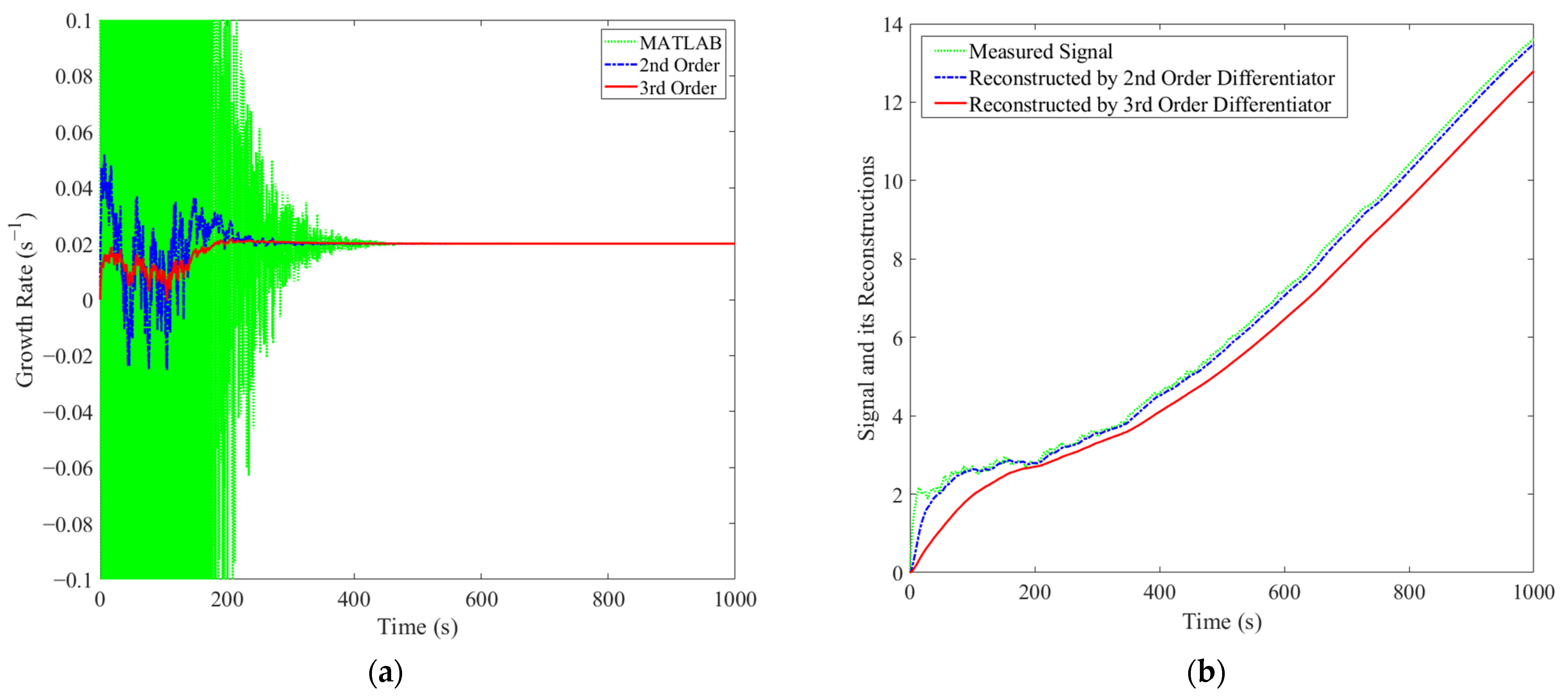
In the simulation, λ = 0.02, the variance of noise w(t) is set to 200. Constant ε of differentiator (26) is chosen as ε = 0.015. From (8), it can be seen that θi (i = 1, …, n; n = 2, 3) is given by constant α, and is set to be α = 0.8. For the 1st-order differentiator, gains ki (i = 1, 2) are given as k1 = 200 and k2 = 1 × 10⁵. For the 2nd-order differentiator, gains ki (i = 1, 2, 3) are set to be k1 = 2000, k2 = 100,200 and k3 = 100,100. The signal derivatives estimated by the 1st- and 2nd-order differentiators given by (26) as well as the Matlab built-in differentiator are all shown in Figure 1a. The simulated signal generated by (37)–(39) and its reconstructions provided by the 1st- and 2nd-order differentiators are all shown in Figure 1b.
From the signal generator given by (37)–(39), if there is no noise, then the signal derivative is λ = 0.02. The effectiveness of a differentiator depends on whether the estimation of signal derivative can converge to λ. In Figure 1a, all the derivatives provided by the 1st-order, the 2nd-order and the Matlab built-in differentiators converge to λ in finite-time, verifying the correctness in designing differentiator (26). The Matlab built-in differentiator is just the derivative block of Simulink, which approximates the derivative of an input signal with a zero initial output. The transfer function of the Matlab built-in differentiator can be written as
where N is the inertia time-constant with a default value of ‘Inf’, i.e., infinitely small. In the simulation, the default value ‘Inf’ is adopted for inertia time-constant N of the Matlab built-in differentiator represented as (40). In Figure 1a, the oscillations during the convergence period of the built-in differentiator are much stronger than those of the 1st- and 2nd-order differentiators, showing that differentiator (26) is more effective than the built-in one for noisy signals. It can be seen from Figure 1a that since inertia time-constant N is infinitely small, the stochastically noised measurement signal is directly differentiated, which caused the serious fluctuation in the signal derivative. Meanwhile, as we can see from (26), the noised measurement is not directly differentiated, and the signal derivative is estimated by the newly-built differentiator with the measurement signal as the input and with integration as the main calculating operation, which effectively suppresses the fluctuation. Moreover, it can be seen from Figure 1a that when the order of the differentiator is higher, the influence of noise is weaker. Actually, we can find the reason from (26). For the 1st-order differentiator, the noise directly affects the estimate of the 1st-order derivative, while the 2nd-order differentiator takes the direct influence of noise into the estimation of the 2nd-order derivative. In Figure 1b, the reconstruction performance of a higher-order differentiator is worse than that of a lower-order one, which is the tradeoff of higher-order. However, since the deviation between the estimation of higher order differentiator and actual signal is constant, threre is no negative influence on the reactor monitoring.
From the above simulaiton results and discussions, differentiator (26) is effective in both time-derivative estimation and signal reconstruction under noisy environments. Moreover, when the order of differentiator is higher, the estimations of derivatives are smoother, but the reconstruction precision is lower.
4.2. Practical Measurement at Low Power-Level
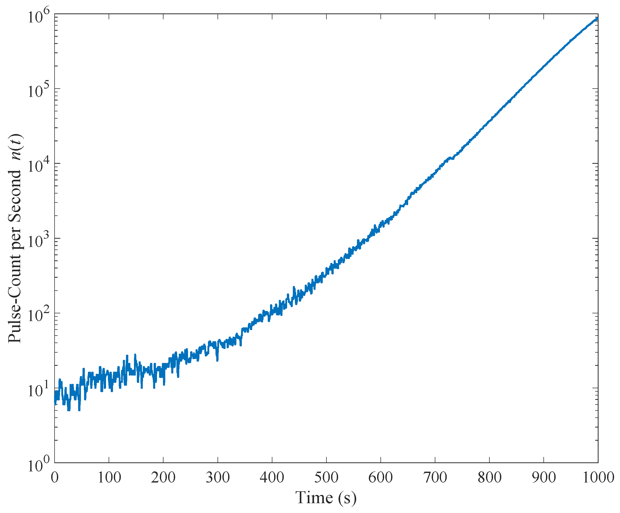
After verifying the feasibility through numerical simulation, differentiator (26) is applied to measure the inverse period of the 5MWth nuclear heating reactor (NHR-5) [20,21] in the startup stage. The NHR-5 is a typical integral pressurized water reactor (iPWR) developed by the institute of nuclear and new energy technology (INET) of Tsinghua University, which has the inherent safety features such as the full-power-range natural circulation, self-pressurization and passive residual heat removing. During the startup of NHR-5 test reactor, the pulse count given by the source range instrument was recorded per second, which is illustrated in Figure 2. To calculate the inverse period or growth rate, the signal adopted to be differentiated is the logarithm of the pulse count after being conditioned by a first-order holder.
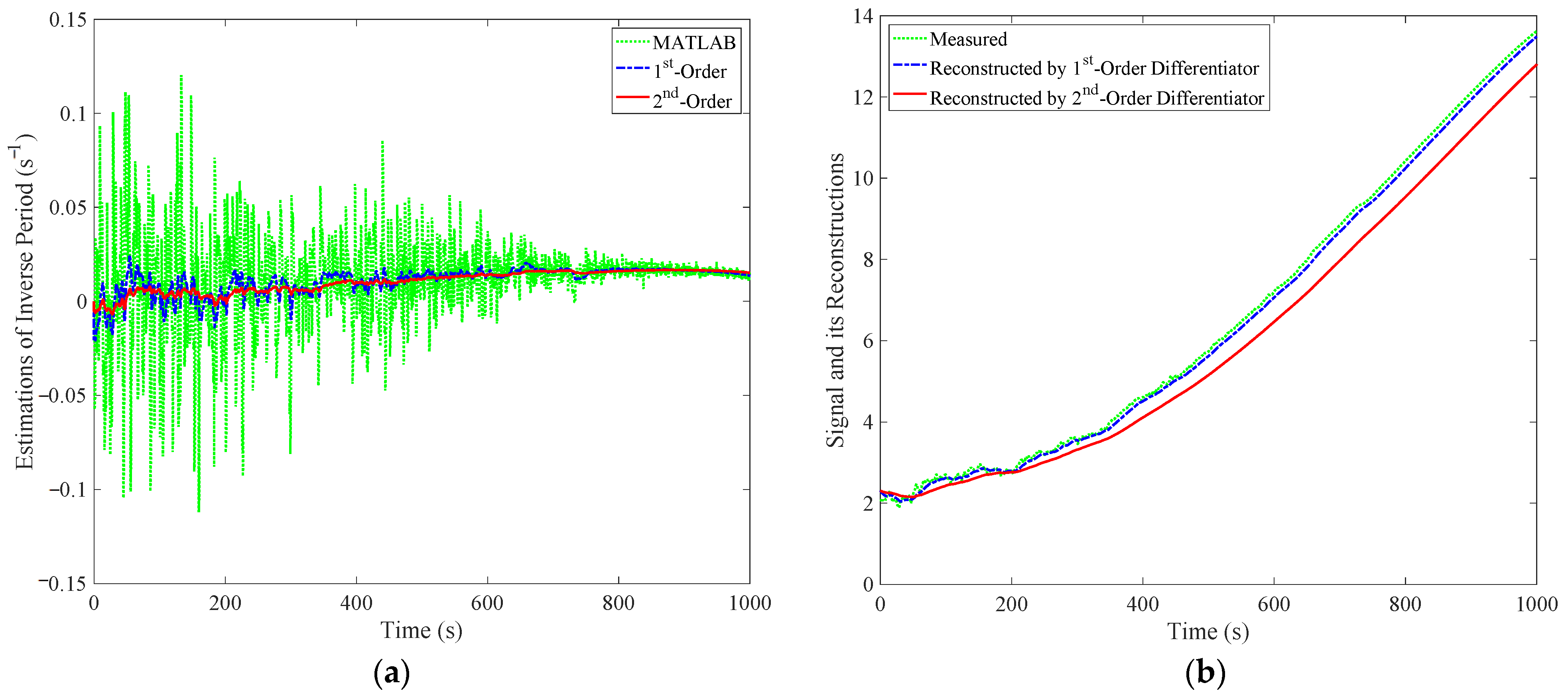
In calculating the inverse period based upon the pulse count, constant ε and gains ki of differentiator (26) are set to the same values as those in the previous numerical simulation, where i = 1, 2 for the 1st-order differentiator, and i = 1, 2, 3 for the 2nd-order differentiator. The estimations of inverse period provided by the Matlab built-in differentiator as well as both the 1st- and 2nd-order differentiators given by (26) are shown in Figure 3a, and the logarithm of pulse count and its reconstructions are shown in Figure 3b.
It can be seen from Figure 2 that when the pulse count rate is low, the fluctuation is strong, which leads to the difficulty in measuring the inverse period in the pulse channel. The fluctuation of neutron flux is mainly given by two types of statistical noises, where one type are the internal noises governed by the statistical nature of neutron interactions, and the other type are the external noises related with random temperature variations and mechanical stresses as well as electronic noises, etc. In Figure 3a, the oscillations in the estimate of the inverse period by the Matlab built-in differentiator is too strong for the differentiator to be adopted practically. Compared to the Matlab built-in differentiator, both the 1st- and 2nd-order differentiators determined by (26) can provide acceptable estimates of inverse period. The reason is the same as that in the numerical simulation. Since the measurement noise is directly differentiated in the Matlab built-in differentiator, there must be a big fluctuation in the estimation of derivative. Meanwhile, it can be seen from (26) that the estimate of the signal derivative given by the (n − 1)th-order differentiator is influenced by the integration of measurement noise directly and by neither the noise itself nor its derivative. Moreover, as we can see from Figure 3b, the smoothness in derivative estimation is the tradeoff of the degradation of signal reconstruction. However, since this degradation is only a small constant deviation to the original signal, there is no negative influence to the reactor monitoring.
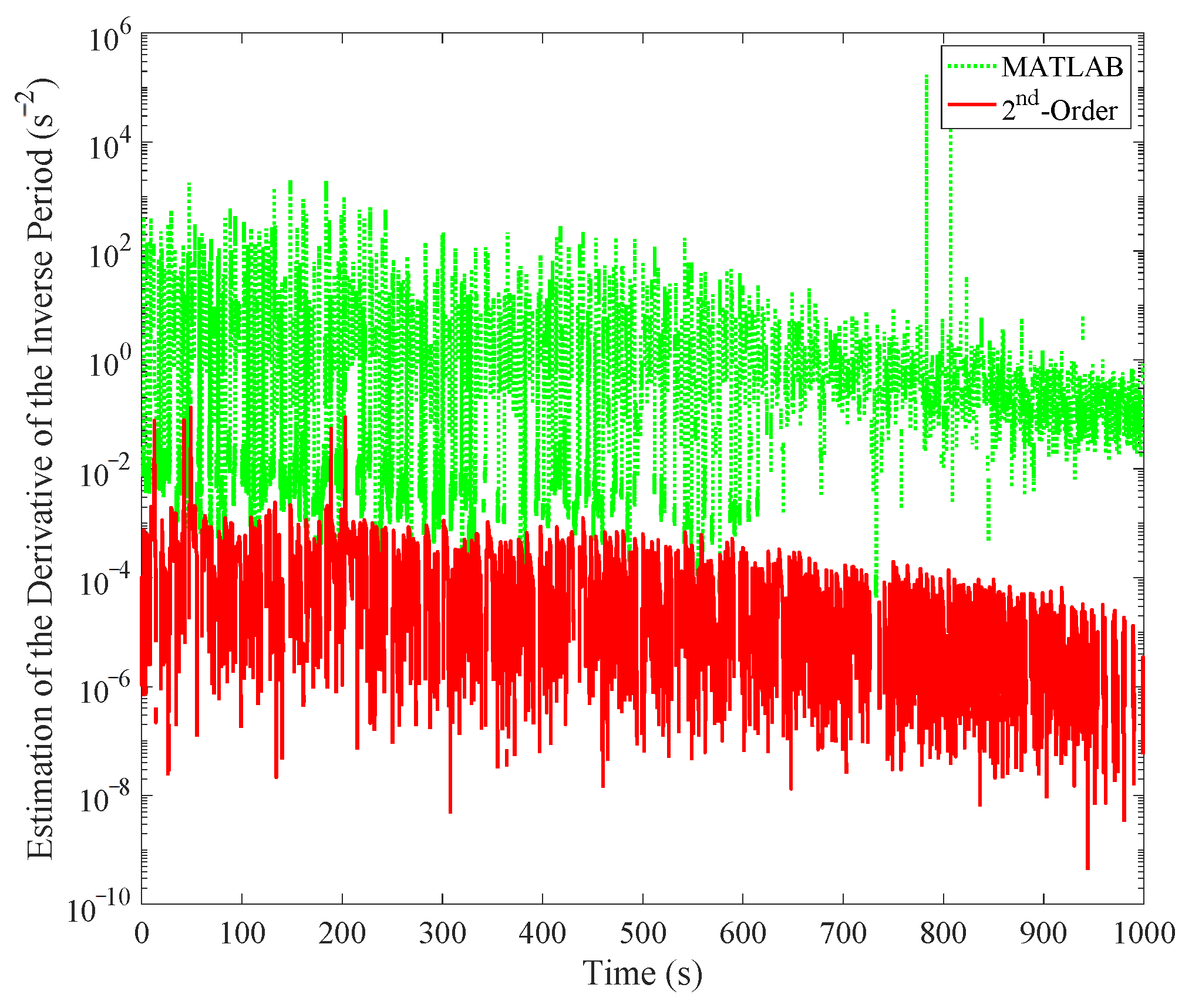
Moreover, the estimations of reactor period and total reactivity that are calculated from the estimations of inverse period by the Matlab built-in differentiator as well as the newly-built 1st- and 2nd-order differentiator are all shown in Figure 4a,b, respectively. The reactivity is calculated by the well-known in-hour equation. The amplitudes corresponding to the estimates of the derivative of inverse-period provided by the Matlab built-in and 2nd-order differentiators are shown in Figure 5. From Figure 4a, the shortest estimated period determined by the built-in differentiator is much smaller than those given by the 1st- and 2nd-order differentiators, which shows the capability of differentiator (26) in triggering fewer false alarms of a short period. From Figure 4b, a higher-order differentiator can enhance the smoothness of the estimate of total reactivity than the lower order one can. Moreover, from Figure 5, because of the influence of strong measurement noise, the derivative of inverse period estimation given by the Matlab built-in differentiator is much larger than that given by the 2nd-order differentiator, further showing that the newly-built differentiator (26) is robust to strong measurement noises, and is feasible to be implemented for the measurement and monitoring of nuclear reactors.
From (26), it can be seen that the newly-built differentiator is essentially a system of ordinary differential equations, and it is easy to be implemented on those widely-used digital control system platforms. Moreover, it is worthy to note that there are no practical difficulties in applying a higher order differentiator taking the form as (26). Actually, if the differentiation given by 2nd-order differentiator is still not satisfactorily smooth, then we can adopt the 3rd or even higher order, which depends on acceptance of performance.
5. Conclusions
The inverse period, i.e., the growth rate of a nuclear fission reactor denotes the fractional increase in the neutron flux per second, which is a key parameter reflecting the safety status of reactors. From the definition given by Equation (1), the inverse period is equal to the derivative of the signal given by the logarithm of neutron flux. Because of the inherent strong statistical fluctuation of neutron flux at low power-levels, it is quite difficult to accurately obtain the signal derivative, especially in the pulse channel. Hence, it is reasonabe to develop signal differentiators that are robust to strong background noises. In this paper, a simple differentiator is newly proposed, which is shown by Lyapunov stability analysis to be finite-time convergent with bounded estimation error. After verifying the theoretical result by numerical simulation, the newly-built differentiator is applied to estimate the inverse period and its derivatives as well as the period and the reactivity of a test reactor from the pulse count data measured in the startup stage. The calculating results show that the performance of this new differentiator is acceptable and much better than the Matlab built-in differentiator, and the estimations can be smoothed by increasing the order of the differentiator. In the future, it is quite meaningful to develop real-time differentiators by implementing algorithm (26) to digital control system platforms such as an embedded computer.
Author Contributions
Conceptualization, Z.D.; methodology, Z.D., Y.Z. (Yunlong Zhu); validation, Y.Z. (Yunlong Zhu); writing—original draft preparation, Y.Z. (Yunlong Zhu); writing—review and editing, Z.D.; data, D.L.; funding acquisition, Z.D., X.H.; project supervision, Y.D., Y.Z. (Yajun Zhang) and Z.Z. All authors have read and agreed to the published version of the manuscript.
Funding
This research was jointly funded by Natural Science Foundation of China (NSFC) (Grant No. 62173202) and National S&T Major Project of China (Grants No. ZX069) And The APC was funded by NSFC (Grant No. 62173202).
Acknowledgments
The authors would like to thank the anonymous reviewers for the constructive comments.
Conflicts of Interest
The authors declare no conflict of interest.
Appendix A
The detailed proof of Lemma 2 is given below.
Let the attraction domain of the origin x = O be denoted by RA, where RA ⊂ D. Based on the converse Lyapunov theorem, there is a smooth positive definite function W(x) and a continuous, positive definite function Q(x) both defined for all x ∈ D, such that
where ∂RA is the boundary of RA, and for any c > 0, {V(x) ≤ c} is a compact subset of RA.
For ∀d > 0, define function V(x) as
where function α satisfies the properties given by
Since system (4) is asymptotically stable around the origin, it can be seen that for any initial point x0 ∈ RA, there exits t1 and t2, such that
From (A2) and (A4), it can be obtained that
which means that V(x) is strictly positive-definite.
Define state-transformation
It can be seen that
Since vector function f is δr-homogenous of degree h,
By substituting Equations (A8) to (A7), system dynamics (4) under transformation (A6) can be written as
Differentiate V(x) along the trajectory of system (4),
which shows that the derivative of V is strictly negative definite. Then, from (A5) and (A10), it can be seen that V(x) is a Lyapunov function of system (4).
Further, it can also be derived that
and
where
From (A11) and (A12), functions V and are δr-homogenous of degree h and d-h, respectively.
Since positive-definite function W(x) is smooth, both functions V and are smooth, which means that there exist positive constants Ck ( k = 1, 2, 3, 4) so that
where Sr,p is just the δr-homogeneous unit sphere introduced in Definition 3.
For ∀z ∈ RA/{O}, it can be seen that
Actually, by the direct calculation, it can be verified that
By substituting (A14) to (A13), and based on the homogeneity property of V and , we have
From inequalities (A16) and (A17), it can also be seen that
where
Since d can be arbitrarily chosen, we set d > h, which gives
Hence, from inequalities (A18) and (A19) as well as Lemma 1, the origin x = O is finite-time stable.
From the smoothness of positive-definite function W(x), it can be seen that
is also smooth, which means that there exist positive constants Di1 and Di2 (i = 1, …, n) so that
Further, from the relationship given by
we can see that function (A20) is δr-homogenous of degree d − ri. By substituting (A14) to (A21), one can find that
Based on (A16) and (A23), if we choose
then inequality can be well satisfied. This completes the proof of Lemma 2.
References
- Vincent, C.H.; Rowles, J.B.; Steels, R.A.W. A precise digital period meter for a nuclear reactor. Nucl. Instrum. Methods 1964, 26, 221–237. [Google Scholar] [CrossRef]
- Scott, E.W.; Stigall, P.D. An accurate digital instrument to measure reactor period. IEEE Trans. Nucl. Sci. 1973, 20, 12–17. [Google Scholar] [CrossRef]
- Mundim, S.G. A digital method for reactor-period measurement. Nucl. Instrum. Method 1974, 118, 273–278. [Google Scholar] [CrossRef]
- Vincent, C.H. Reactor-period measurements at low powers. Electron. Lett. 1974, 10, 475–476. [Google Scholar] [CrossRef]
- Khalil, H.K. Robust servomechanism output feedback controllers for feedback linearizable systems. Automatica 1994, 30, 1587–1599. [Google Scholar] [CrossRef]
- Dabroom, A.M.; Khalil, H.K. Discrete-time implementation of high-gain observers for numerical differentiation. Int. J. Control 1999, 72, 1523–1537. [Google Scholar] [CrossRef]
- Ibrir, S. On continuous time differentiation observers. In Proceedings of the European Control Conference, Karlsruhe, Germany, 31 August–3 September 1999. [Google Scholar]
- Ibrir, S. Linear time-derivative trackers. Automatica 2004, 40, 391–405. [Google Scholar] [CrossRef]
- Levant, A. Robust exact differentiation via sliding mode technique. Automatica 1998, 34, 379–384. [Google Scholar] [CrossRef]
- Levant, A. High-order sliding modes, differentiation and output-feedback control. Int. J. Control 2003, 76, 924–941. [Google Scholar] [CrossRef]
- Han, J. From PID to active disturbance rejection control. IEEE Trans. Ind. Electron. 2009, 56, 900–906. [Google Scholar] [CrossRef]
- Xue, W.; Huang, Y.; Yang, X. What kinds of system can be used as tracking-differentiator. In Proceedings of the 29th Chinese Control Conference, Beijing, China, 29–31 July 2010. [Google Scholar]
- Guo, B.; Zhao, Z. On the convergence of tracking differentiator. Int. J. Control 2011, 84, 693–701. [Google Scholar] [CrossRef] [Green Version]
- Guo, B.; Zhao, Z. Weak convergence of nonlinear high-gain tracking differentiator. IEEE Trans. Autom. Control 2013, 58, 1074–1080. [Google Scholar] [CrossRef]
- Wang, X.; Chen, Z.; Yang, G. Finite-time-convergent differentiator based on singular perturbation technique. IEEE Trans. Autom. Control 2007, 52, 1731–1737. [Google Scholar] [CrossRef]
- Hong, Y.; Huang, J.; Xu, Y. On an output feedback finite-time stabilization problem. IEEE Trans. Autom. Control 2001, 46, 305–309. [Google Scholar] [CrossRef] [Green Version]
- Hong, Y. Finite-time stabilization and stabilizability of a class of controllable systems. Syst. Control Lett. 2002, 46, 231–236. [Google Scholar] [CrossRef]
- Dong, Z. A two-order finite-time-convergent differentiator with application to nuclear reactors. In Proceedings of the 14th International Conference on Control, Automation, Robotics and Vision, Phuket, Thailand, 13–15 November 2016. [Google Scholar]
- Bacciotti, A.; Rosier, L. Liapunov Fuctions and Stability in Control Theory, 2nd ed.; Springer: Berlin, Germany, 2005; pp. 181–186. [Google Scholar]
- Wang, D. The design characteristics and construction experiences of the 5 MW nuclear heating reactor. Nucl. Eng. Des. 1993, 143, 19–24. [Google Scholar]
- Wang, D.; Zhang, D.; Dong, D.; Gao, Z.; Li, H.; Lin, J.; Su, Q. Experimental study and operation experiences of the 5MW nuclear heating reactor. Nucl. Eng. Des. 1993, 143, 9–18. [Google Scholar]
Figure 1.
Numerical simulation results for the estimations of the derivative of a given signal provided by different differentiators: (a) growth rate, (b) measured and reconstructed signals.
Figure 1.
Numerical simulation results for the estimations of the derivative of a given signal provided by different differentiators: (a) growth rate, (b) measured and reconstructed signals.

Figure 2.
Practical measured pulse count per second.

Figure 3.
Measurements of inverse period given by different differentiators: (a) estimations of inverse period, (b) signal and its reconstructions.
Figure 3.
Measurements of inverse period given by different differentiators: (a) estimations of inverse period, (b) signal and its reconstructions.

Figure 4.
Estimations of reactor period and total reactivity given by different differentiators: (a) reactor period, (b) reactivity.
Figure 4.
Estimations of reactor period and total reactivity given by different differentiators: (a) reactor period, (b) reactivity.

Figure 5.
Amplitude of the derivative of the inverse period.

Publisher’s Note: MDPI stays neutral with regard to jurisdictional claims in published maps and institutional affiliations. |
© 2022 by the authors. Licensee MDPI, Basel, Switzerland. This article is an open access article distributed under the terms and conditions of the Creative Commons Attribution (CC BY) license (https://creativecommons.org/licenses/by/4.0/).
Share and Cite
MDPI and ACS Style
Zhu, Y.; Dong, Z.; Li, D.; Huang, X.; Dong, Y.; Zhang, Y.; Zhang, Z. A Finite-Time Differentiator with Application to Nuclear Reactor Inverse Period Measurement. Energies 2022, 15, 4487. https://doi.org/10.3390/en15124487
AMA Style
Zhu Y, Dong Z, Li D, Huang X, Dong Y, Zhang Y, Zhang Z. A Finite-Time Differentiator with Application to Nuclear Reactor Inverse Period Measurement. Energies. 2022; 15(12):4487. https://doi.org/10.3390/en15124487
Chicago/Turabian StyleZhu, Yunlong, Zhe Dong, Duo Li, Xiaojin Huang, Yujie Dong, Yajun Zhang, and Zuoyi Zhang. 2022. "A Finite-Time Differentiator with Application to Nuclear Reactor Inverse Period Measurement" Energies 15, no. 12: 4487. https://doi.org/10.3390/en15124487
Note that from the first issue of 2016, this journal uses article numbers instead of page numbers. See further details here.