
Stability Boundary Analysis of Islanded Droop-Based Microgrids Using an Autonomous Shooting Method


AAU Energy, Aalborg University, Pontoppidanstræde 111, 9220 Aalborg, Denmark
*
Author to whom correspondence should be addressed.
Energies 2022, 15(6), 2120; https://doi.org/10.3390/en15062120
Submission received: 8 February 2022
/
Revised: 3 March 2022
/
Accepted: 10 March 2022
/
Published: 14 March 2022
(This article belongs to the Section A1: Smart Grids and Microgrids)
Abstract
:This paper presents a stability analysis for droop-based islanded AC microgrids via an autonomous shooting method based on bifurcation theory. Shooting methods have been used for the periodic steady-state analysis of electrical systems with harmonic or unbalanced components with a fixed fundamental frequency; however, these methods cannot be directly used for the analysis of microgrids because, due to the their nature, the microgrids frequency has small variations depending on their operative point. In this way, a new system transformation is introduced in this work to change the droop-controlled microgrid mathematical model from an non-autonomous system into an autonomous system. By removing the explicit time dependency, the steady-state solution can be obtained with a shooting methods and the stability of the system calculated. Three case studies are presented, where unbalances and nonlinearities are included, for stability analysis based on bifurcation analysis; the bifurcations indicate qualitative changes in the dynamics of the system, thus delimiting the operating zones of nonlinear systems, which is important for practical designs. The model transformation is validated through time-domain simulation comparisons, and it is demonstrated through the bifurcation analysis that the instability of the microgrid is caused by supercritical Neimark–Sacker bifurcations, and the dynamical system phase portraits are presented.
1. Introduction
The adaptability and resilience of a microgrid (MG) are two of the desired features due to the multiple operational scenarios that the system can meet [1]. Because of this, the control requirements and strategies to perform local balancing and to maximize their benefits have led the MGs to fulfill a wide range of functionalities, such as power flow control, voltage and frequency regulation, among others [2,3,4]. In this way, the choice of control structure is important for the stable operation of microgrids, which is achieved by means of different control levels, also known as hierarchical controls [2]. MG controls are usually divided into three levels of control structure, primary control, secondary control, and tertiary control. Generally, they have different control objectives and timescales. The primary control level is responsible for performing the grid-forming or grid-feeding function. For the islanded case, grid-forming controls, for example the droop control, are required to regulate the frequency and voltage of the microgrid [5]; however, these controls usually require the introduction of a secondary control to eliminate the steady-state errors [3]. On the other hand, the tertiary control is used to decide the operating point of each distributed generation unit (DG), i.e., energy management systems (EMS) [4], depending on the grid requirements and available energy. Therefore, the primary and secondary controls in microgrids are continually optimized by using upper control layers, such that, the operational objectives are continuously achieved in a reliable manner [3,6]. This means that, in the design stage, the microgrid has to be tested not only for one set of control characteristics, but for operational regions, which will set boundaries for the optimizations and the system operation.
Conventional stability analyses in microgrids are based on eigen-analysis [7]. In these analyses, the steady-state solution of the system represented by a set of autonomous ordinary differential equations, i.e., , is simply to solve , then, the stability of the system is obtained by linearizing around the computed equilibrium points; average models fall within this type of systems. Alternatively, fast-time domain methods, also known as shooting methods [8], have been used in the literature for electrical systems harmonic analysis and unbalanced systems, including the detailed modeling of the close-loop controls and nonlinear elements. In these methods, the solution can be represented as a two-point boundary-value problem, assuming that the periodic steady-state solution has a fundamental period T, such that the is satisfied in steady state [9,10,11,12]. In [9], the modeling and analysis of an adjustable speed driver (ASD) is performed, where the state-space formulation of the ASD explicitly includes the switching process in the diode rectifier and the inverter; in this work, the periodic steady-state computation is performed via the discrete exponential expansion method. The steady-state computation of a fixed-speed wind turbine is performed in [10]; the authors present the detailed modeling of the wind turbine, and the periodic steady-state calculation is performed using the numerical differentiation method for different operational conditions. Additionally, the results are compared against the brute force approach to show the advantages of the shooting method. In [11], the periodic steady-state solution of an electric system with unified power-flow controllers (UPFCs) is presented. The steady-state solution is computed using the numerical differentiation method and a harmonic analysis of the system is performed. Recently in [12], the authors perform a harmonic assessment of an islanded microgrid using different shooting methods, furthermore, the shooting methods are compared in terms of their computational efficiency. The results obtained with the shooting methods are compared against simulations performed in the professional software PSCAD.
Note that, to explore both stable and unstable system solutions given by the aforementioned methods, a suitable framework is the bifurcation analysis. A bifurcation is a qualitative change in the dynamics of the system, under the variation of one or more parameters on which the system depends [13]. The application of the bifurcation theory has been performed for studies such as, voltage collapse [14], flexible AC transmission system devices [15], sub-synchronous resonances [16], among others [17]. Furthermore, the analysis of microgrids with different controls using the bifurcation theory has been presented in recent works [18,19,20,21,22,23,24,25,26]. The stability analysis of a synchronverter-dominated microgrid based on bifurcation theory was presented in [18]; in this work, the system is modeled in DQ frame and an eigenvalue analysis is performed considering three different bifurcation paramenters, additionally, the results show that the modification of the reactive power coefficient provokes a Hopf bifurcation in the system. In [19], the local stability of droop-controlled inverter-based microgrids with dynamic loads was studied; a two-machine test system is modeled and implemented in AUTO, which is a professional software used for computing equilibrium branches and bifurcation points. In [20], the computation of stability regions in an islanded droop-controlled microgrid is performed through a bifurcation analysis software called MATONT; the system is modeled in DQ reference frame, and different load types are considered. It is found in this work that the power controllers and loads have a major influence in the bifurcations. An stability analysis for converter-based DC microgrids with constant power loads is assessed in [21]; in this work, a linearized small-signal model is used to compute the stability behavior in the system against different changes further finding Hopf bifurcations. In [22], a bifurcation analysis of a microgrid with constant power loads is performed; for this work, a reduced order model is considered and the system stability is analyzed for different load powers, the results are compared against simulations using the complete microgrid system, showing that the control gains affect the stability of the system and that Hopf bifurcations appear in some cases. In [23], a continuation method is used to identify Hopf bifurcations in an islanded microgrid considering distributed energy resources and electric vehicle charging stations; for this purpose, a load increase is selected as bifurcation parameter and the system is linearized at each equilibrium point. The unstable points are obtained and the Hopf bifurcation points verified via time-domain simulations. A generalized model is proposed in [24], this model is given by a block diagram approach used for modeling the microgrid, then the system initialization is obtained via a load flow method and the eigenvalues are computed, bifurcation analyses and phase diagrams are presented showing the Hopf bifurcations under different cases. Two saddle-node bifurcation point algorithms for islanded microgrids are presented in [25], these approaches use the power flow method as base to obtain the feasible and non-feasible operational regions after an increase of load in the system, then, the proposed algorithms are used to search between these regions the saddle-node bifurcation; to verify the algorithms, four case studies are implemented and comparisons among traditional methods presented. Recently in [26], the bifurcation analysis was used to predict the parameter stability margins with and without secondary control in islanded droop-controlled microgrids; in this work, the system is modeled in the DQ reference frame and an eigenvalue analysis is performed considering different parameters. The authors showed that the MG stability is sensitive to several parameters such as droop gains, proportional/integral PI controller coefficients, among others, and that the inverter-based MG may lose its stability through a Hopf or saddle-node bifurcation.
Note that in the aforementioned works for microgrids, only the fundamental frequency is considered and the MGs are modeled in the DQ reference frame or the system model is reduced, therefore unbalances in the system and harmonic components are overlooked. In practice, the operation of a microgrid includes unbalances and harmonic components, for this reason, fundamental frequency methods cannot always be used to compute the steady-state solution in a reliable way, and there is a need for more detailed algorithms. As mentioned before, the shooting methods can be used for electrical systems harmonic analysis and unbalanced systems; however, since these methods calculate the periodic steady-state solution, they require a known fundamental period, i.e., a fixed system frequency. In this way, these methods cannot be directly used for the analysis of MGs because, due to the their operative nature, the MGs frequency has small variations depending on their operative point.
In order to cope with this issue, in this work the MG mathematical model can is transformed from a non-autonomous system into an autonomous system. By removing the explicit time dependency, the steady-state solution can be obtained with a shooting method and the stability of the system calculated such that the shooting methods can compute the steady-state solution even with variable and unknown frequency. In this way, in this contribution, by including a mathematical system transformation, a shooting method is used to perform the bifurcation analysis, which allows the consideration of the system nonlinear dynamics, unbalances, and the harmonic content. With these explanations, the main contributions of this paper are summarized as follows:
- Introducing a model transformation for droop-controlled MGs, such that the original non-autonomous system model becomes an autonomous system, removing in this way the explicit time dependency.
- The use of the discrete exponential expansion method for the computation of the periodic steady-state solution in autonomous systems.
- The bifurcation analysis of the droop-controlled MG is presented under three-case studies: (1) droop characteristic variation for fundamental frequency; (2) unbalanced load variation for fundamental frequency; and (3) droop characteristic variation including the converters commutation process.
- A stability boundary map is created using the proposed approach, and phase portraits are presented showing the torus attractors made by the Neimark–Sacker bifurcations.
The paper is organized as follows: Section 2 describes the periodic steady-state solution formulation for autonomous systems, where also the discrete exponential expansion method is presented. Section 3 introduces the primary droop control and presents the procedure for the system transformation from a non-autonomous to an autonomous system. Section 4 describes the microgrid used as the test system, and the validation of the transformed system with and without commutations is performed. Section 5 outlines the case studies and presents results obtained. Section 6 presents a discussion. Finally, Section 7 provides the conclusions of this work.
2. Periodic Steady-State Solution Formulation for Autonomous Systems
In general, the mathematical model of a controlled microgrid can be given by the following ordinary differential equation set,
where is the state vector of n elements and t is the time.
A way to compute the steady-state solution of a controlled system represented by a set of ordinary differential equations such as (1), is to find a state vector such that , where T is the fundamental period of the system, is the state vector at and =(, ; ).
This problem can be addressed through fast-time-domain methods [8,27]; however, for microgrids without frequency compensation controls, these methods cannot be directly used because the fundamental period of the system is unknown, and changing with the operation of the system. Nonetheless, if a periodic system do not explicitly depend on the time, i.e., an autonomous system, this problem can be overcome even if the system period is unknown, by using autonomous shooting methods. The formulation of these methods is presented as follows.
2.1. Autonomous Systems
The mathematical model of an autonomous systems is given by the following equation set [13],
note that the state function is not time dependent as in (1). If the system is periodic, its solution can be represented as a two-point boundary-value problem with the period determined along with the states, as shown below,
where is the state vector in steady-state and is the solution after one full cycle T. In order to compute the values of and T, a correction is accomplished through the Newton–Raphson method.
Therefore, to compute the corrections, (5) is expanded in a Taylor series and only the linear terms are kept as follows:
where is an matrix, is the identity matrix, and is an vector. Observe that (6) constitutes a system of n equations but unknowns, thus, an extra equation is needed. On the other hand, an autonomous system periodic solution is invariant to linear shifts in the time origin, i.e., if is a solution, then is also a solution for any arbitrary , this means that the phase is arbitrary. In this case, to remove the arbitrariness, an orthogonality phase condition equation [13] is used, which sets a requirement for the correction to be normal to the vector field, and it completes the system (6), that is,
Using this condition equation, the following system of equations is obtained:
after determining the corrections, a convergence criterion is checked. If the criterion is not satisfied, the initial guess is updated as and the procedure is repeated.
Note in (8), that the matrix evaluated at have to be computed in order to find the corrections. For this purpose, several numerical methods have been presented in the literature, where each method differs on how the approximation is performed. In this work, the discrete exponential expansion method is used since it presents a good convergence rate and the best computational time performance from the other methods [12].
2.2. Discrete Exponential Expansion Method
The discrete exponential expansion (DEE) method was proposed in [28]. It follows an identification procedure step-by-step based on a recursive formulation, that requires the integration of only one full cycle for the computation of the transition matrix. This method approximates the matrix as,
where the Jacobian is given by,
where is defined as , N is the number if intervals in a period T, and represents the i-th element of the time vector from t to . Once the matrix evaluated at is computed, the corrections and from (8) can be determined and the procedure repeated until the desired convergence error. It should be noticed that the eigenvalues of the Jacobian are the Floquet multipliers [13]; therefore, the stability of the computed solution can be used to obtain the stability of the periodic solution of the system [29], i.e., if the Floquet multipliers are inside the unit circle in the complex plane Z the system is stable, otherwise unstable.
Keep in mind that this method can only be used for periodic autonomous systems with the form of (2), therefore, for the microgrid problem there is still a need for a system transformation, this is presented below.
3. Droop Control System Transformation
The schematic of the conventional droop control incorporated in the AC DG units is shown in Figure 1.
In this control, the active and reactive power contribution of the DG unit depends on the frequency/active power (P−) and voltage/reactive power (Q− V) droop characteristic curves, respectively [6,30],
where is the nominal angular frequency of the system, is the voltage amplitude reference, and are the P − and Q − V droop coefficients, respectively, and P and Q are the output active and reactive power, respectively. Additionally, this control includes an inner current control loop and an outer voltage control loop, which define the control signals for operating each DG unit with a given voltage amplitude and frequency.
Note in Figure 1 the explicit time dependency in this control can be found in the integration block from the droop control for computing , which is given by,
This means that the computation of has to be performed in a different way in order to avoid the system time dependency. If the control is analyzed, it can seen that is required for performing the DQ-abc and abc-DQ transformations, (14) and (15).
Even more, inspecting the transformation equations, it can be seen that is always used for computing sine or cosine, with or without a phase shift. Therefore, it is possible to numerically compute and without the time dependency. It is known that,
If sine and cosine are represented by a numerical variable, the previous equations turn into,
where is given by (11) from the droop control. Then, the phase shifting needed in some terms of the DQ-abc and abc-DQ transformations can be computed by trigonometric equivalents, such as,
where the term and will be substituted by the terms C and S, respectively. Therefore, with these changes, the DQ-abc and abc-DQ transformations become (22) and (23); note that the explicit time dependency has been removed from the droop control, becoming an autonomous system.
For the implementation of the control including the transformation, the control block diagram changes as shown in Figure 2. As seen in this block diagram, only the active power computation is modified, such that the output of the active power block is not but and , which are used for the other parts in the control.
Note that with this transformation, the explicit time dependency in the terms and is avoided, and therefore the C and S terms help to turn the mathematical system model into the general autonomous form shown in (2). Then, as presented before, with this transformation the autonomous fast-time domain method can be used to compute the periodic steady-state solution and the stability of the system, even with variable and unknown frequency, for a detailed MG model which can include unbalances, nonlinear dynamics, and the commutation process.
4. Microgrid Test System and Model Validation
Figure 3 shows the test system used in this work. It consists of two distributed generation (DG) units interfaced with voltage source converters (VSC) including a LC filter, connected through feeders to a load.
The primary control of each DG unit is based on the conventional droop control scheme. Table 1 summarizes the nominal parameters selected for the case study as well as the parameters of the inner and the outer control loops at the primary control level. Please note that, for all DG units in this work, for both PI controllers in each loop (current and voltage) the parameters are the same. Furthermore, since the computation of the nominal control parameters is out of the scope of the paper, they were taken from [31].
Test System Model Validation
In this subsection, the autonomous test system which includes the transformation presented in Section 3 is validated by comparing it with the original non-autonomous test system. For this comparison, a load of 100 kW is included via a resistance model; the rest of the system parameters are as showed in Table 1.
In Figure 4, the comparison of the autonomous test system against the non-autonomous test system is presented. In (a), the comparison of the DG1 output current signals for fundamental frequency is shown; in (b), the comparison of the DG1 output current signals for the commutated model is shown; and in (c), the comparison of the active power injected to the load for the commutated case is shown. Note that the simulation results from both autonomous and non-autonomous systems are practically the same for both transient and steady-state; to corroborate this, the mean squared error (MSE) value is calculated for the signals obtained as follows,
where n is the number of elements, Y is the original signal, and is the new signal.
For the fundamental frequency approach, the mean squared error comparing the currents shown in Figure 4a is 3.09 . For the commutated approach, the mean squared error comparing the currents shown in Figure 4b is 1.21 . As expected, the transformation kept the information of the complete original model, even when a high frequency commutation process is enabled. From the results obtained in the comparison, the model including the system transformation presented in Section 3 is validated.
5. Bifurcation Assessment Based on the Autonomous Shooting Method
In this section, three case studies are presented for analyzing the stability of the system under different conditions: (1) a variation of the droop characteristics in the DG1 control in fundamental frequency; (2) unbalancing the system in fundamental frequency; and (3) a variation of the droop characteristics in the DG1 control considering the converters commutation process. For each scenario, the periodic steady-state solution is computed using the shooting method, and the stability information is given by the system Jacobian, which is computed during the solution of the shooting method. Furthermore, for interested readers, supplementary results from the case studies are presented in the Appendix A, where the DGs controlled voltage, injected active power, and system frequency are shown.
5.1. Droop Characteristic Variation
In Figure 5, the Floquet multipliers (the eigenvalues of the Jacobian) due to the droop characteristics variation in the DG1 control is shown. As it can be seen in this figure, it is found that the system becomes unstable via a pair of complex Floquet multipliers leaving the unit circle away from the real axis, which means this system has a Neimark–Sacker bifurcation [13]. The Neimark–Sacker bifurcation essentially introduces a new frequency with the first one in the bifurcating solution. This solution may be periodic or two-period quasiperiodic, depending on the relationship between the newly introduced frequency and the frequency of the periodic solution that existed before. The Neimark–Sacker bifurcation can be subcritical or supercritical, a branch of stable quasiperiodic solutions is created if the bifurcation is supercritical, and a branch of unstable quasiperiodic solutions is destroyed if the bifurcation is subcritical, i.e., a catastrophic bifurcation [13].
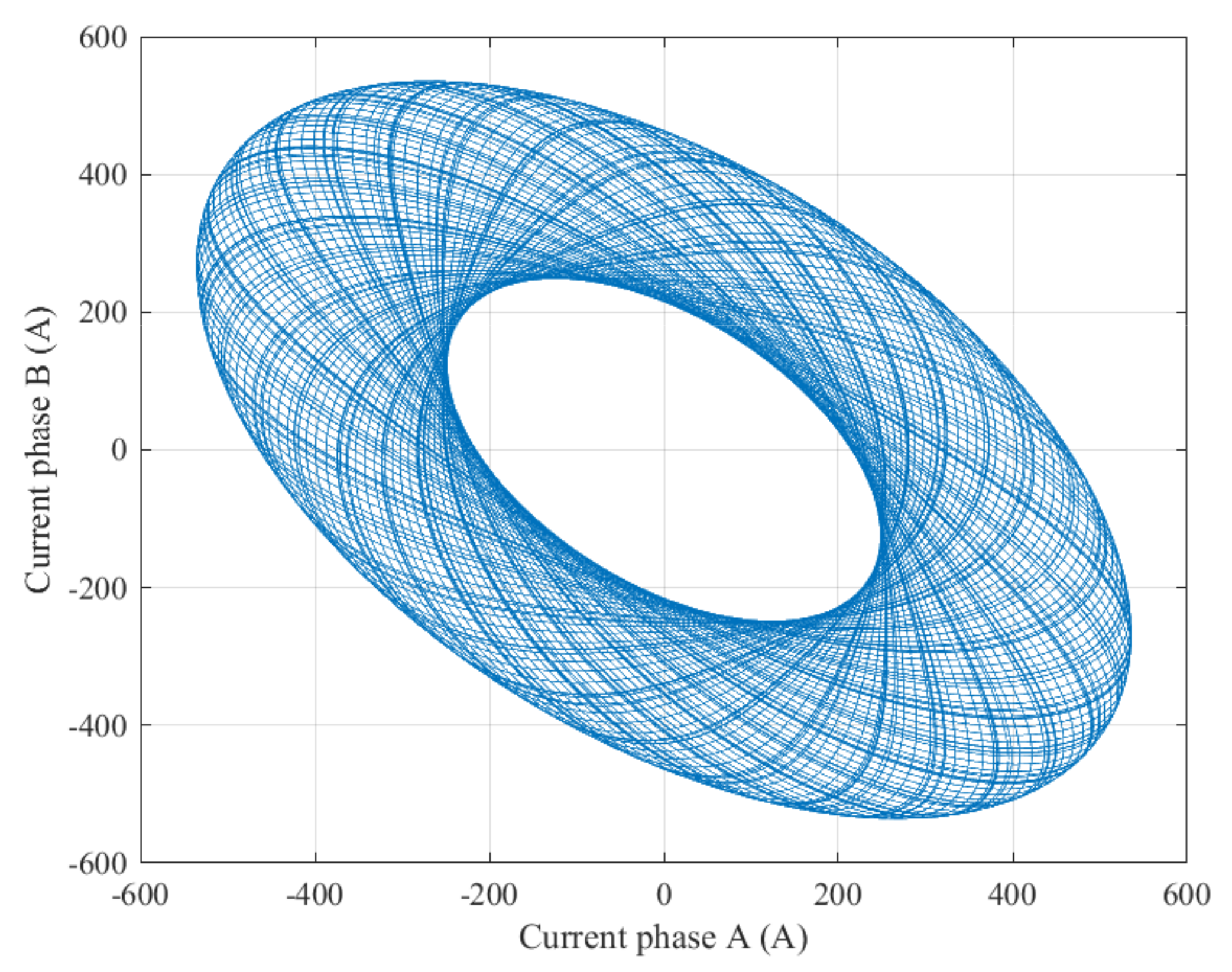
In order to know which bifurcation it is in this case, the system is simulated using the solution given by the shooting method in the point of instability (when the Floquet multipliers fall outside the unit circle), and the resulting phase portrait is shown in Figure 6. Note how the solution oscillates without collapsing the system, this is because in the Neimark–Sacker bifurcation a torus attractor is formed and the solution oscillates around it, which means that a supercritical Neimark–Sacker bifurcation occurred.
Stability Boundary Map
Another asset of the proposed approach using the shooting method is that, if two or more bifurcation parameters are selected, the stability analysis can be repeated for a matrix of values and stability boundary maps can be created for specific bifurcation variables, delimiting the system operating zones. To show this, the droop characteristics and in DG1 are taken as bifurcation variables. Figure 7 shows an operational boundary map, and as explained in Section 2.2, if the absolute Floquet multiplier value becomes bigger than 1, the system is unstable, otherwise, stable. For this case, the possible combinations of and that keep the system stable are presented.
5.2. Load Unbalance Variation
In this case study, a load variation is made only in the phase C such that the system becomes unbalanced. The steady-state solution is obtained using the autonomous shooting method and the stability computed. The Floquet multipliers obtained from the phase C resistance variation are shown in Figure 8; as can be seen in this figure, the system do not become unstable due to the unbalance in the load, however the Floquet multipliers slowly move toward the outside of the unit circle.
5.3. Droop Characteristic Variation with the Converters Commutation Process Enabled
In this case, the same variation in the droop characteristics as in the subsection A is performed, the only difference is that the converters commutation process is enabled. It is worth mentioning that in order to avoid convergence problems of the shooting method and numerical oscillations, the switching functions are modeled using an hyperbolic tangent approach introduced in [32].
In Figure 9, the Floquet multipliers due to the droop characteristics variation in the DG1 control is shown. It is found again that the system becomes unstable via a pair of complex Floquet multipliers, which means this system has a Neimark–Sacker bifurcation; however, in this case the system becomes unstable before () as compared with the fundamental frequency case. On the other hand, it can be seen that the Floquet multipliers trajectory dynamics are completely different from the previous case.
These differences show that by considering the commutation in the DG units, the dynamics of the system change considerably, further affecting not only the overall system power quality but the system stability against changes in the control and the grid parameters. Since in practice the harmonic phenomena is always present in power-electronic-based power systems, it is clear that the consideration of the harmonic content is necessary during design and stability analyses.
As in the first case, in order to know which type of Neimark–Sacker bifurcation it is, the system simulation using the unstable solution found with the autonomous shooting method is required. Figure 10 shows the resulting phase portrait from the simulation. Note in this figure that the solution forms a torus, as in the first case, which means that the instability is given by a supercritical Neimark–Sacker bifurcation; however, observe that both phase portraits from the first case and this case are not similar, this is because, as discussed before from the Floquet multipliers results, the system dynamics before and after enabling the commutation process in the DG units are different and the unstable solution has a different dynamic, showing again the need to consider detailed system models for the system assessment.
6. Discussions
The obtained results showed the reliability of the proposed transformation and the usefulness of the shooting method for the computation of the periodic steady-state solution of droop-controlled MGs with variable and unknown frequency. It is important to highlight the advantages of the autonomous shooting method, since it allowed the consideration of the detailed controlled microgrid for both fundamental frequency and enabling the power electronic devices commutation, furthermore, it also allows nonlinear components and unbalances in the system, which cannot be considered in the conventional small-signal stability approaches. On the other hand, the disadvantage of this method is that the computing time could be restrictive for multiple calculations, i.e., for computing stability maps, even though parallel computing techniques can be included to improve the computing time. Nevertheless, the method presented in this work, including the necessary system transformation, is a reliable and flexible alternative for detailed islanded microgrids stability analyzes. Furthermore, it was shown during the stability analysis that the dynamics of the MG change considerably if the commutation of the power electronic devices is considered. Therefore, the need for the use of detailed models during the design stage and stability analysis is highlighted.
7. Conclusions
A detailed microgrid system, considering multiple aspects such as, nonlinearities, unbalances and closed-loop controls was used as case study in order to perform stability analyzes based on an autonomous shooting method. Since the microgrid is mathematically represented by a non-autonomous system with variable frequency, a system transformation was introduced which allowed the use of an autonomous shooting method. The transformation was validated through simulation comparisons in both fundamental frequency and enabling the converters commutation.
The presented results revealed the suitability of the proposed transformation, and the reliability of the autonomous shooting method for computing the steady-state solution and stability of the system. In the case studies, the bifurcation analyzes showed that the microgrid becomes unstable due to a Neimark–Sacker bifurcation, furthermore, with the phase diagrams assessment it was concluded that the bifurcation was more specifically a supercritical Neimark–Sacker bifurcation, which means that a torus attractor is formed and the system solution oscillates around it.
Author Contributions
Conceptualization, G.D.A.-T.; methodology, G.D.A.-T.; software, G.D.A.-T.; validation, G.D.A.-T.; formal analysis, G.D.A.-T.; investigation, G.D.A.-T.; resources, J.C.V. and J.M.G.; writing—original draft preparation, G.D.A.-T.; writing—review and editing, G.D.A.-T., J.C.V. and J.M.G.; visualization, G.D.A.-T.; supervision, J.C.V. and J.M.G.; project administration, J.C.V. and J.M.G.; funding acquisition, J.C.V. and J.M.G. All authors have read and agreed to the published version of the manuscript.
Funding
This work was funded by a Villum Investigator, grant no. 25920, from The Villum Fonden.
Institutional Review Board Statement
Not applicable.
Informed Consent Statement
Not applicable.
Data Availability Statement
Not applicable.
Conflicts of Interest
The authors declare no conflict of interest.
Appendix A
In this appendix, supplementary results from the case studies are shown. In particular, the DGs controlled voltage, the active power injected by the DGs, and the system frequency.
Appendix A.1. Case 1: Droop Characteristic Variation
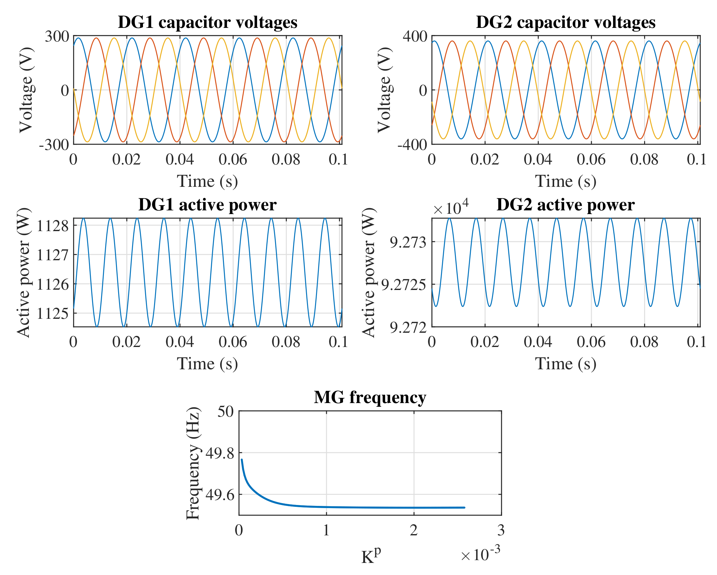
Using the obtained controlled-MG model, a time-domain simulation is performed and the results from five cycles are presented in Figure A1. In particular, the DGs controlled voltage and the active power injected by the DGs are shown. Furthermore, the system frequency during the whole variation is presented as well. It is worth mentioning that for this simulation, the initial state-vector used was the unstable solution computed via the autonomous shooting method for the Case 1.
Figure A1.
Time-domain simulation of five full-cycles of the computed unstable solution in Case 1, before the system collapses. Additionally, the system frequency during the whole variation.
Figure A1.
Time-domain simulation of five full-cycles of the computed unstable solution in Case 1, before the system collapses. Additionally, the system frequency during the whole variation.

Appendix A.2. Case 2: Load Unbalance Variation
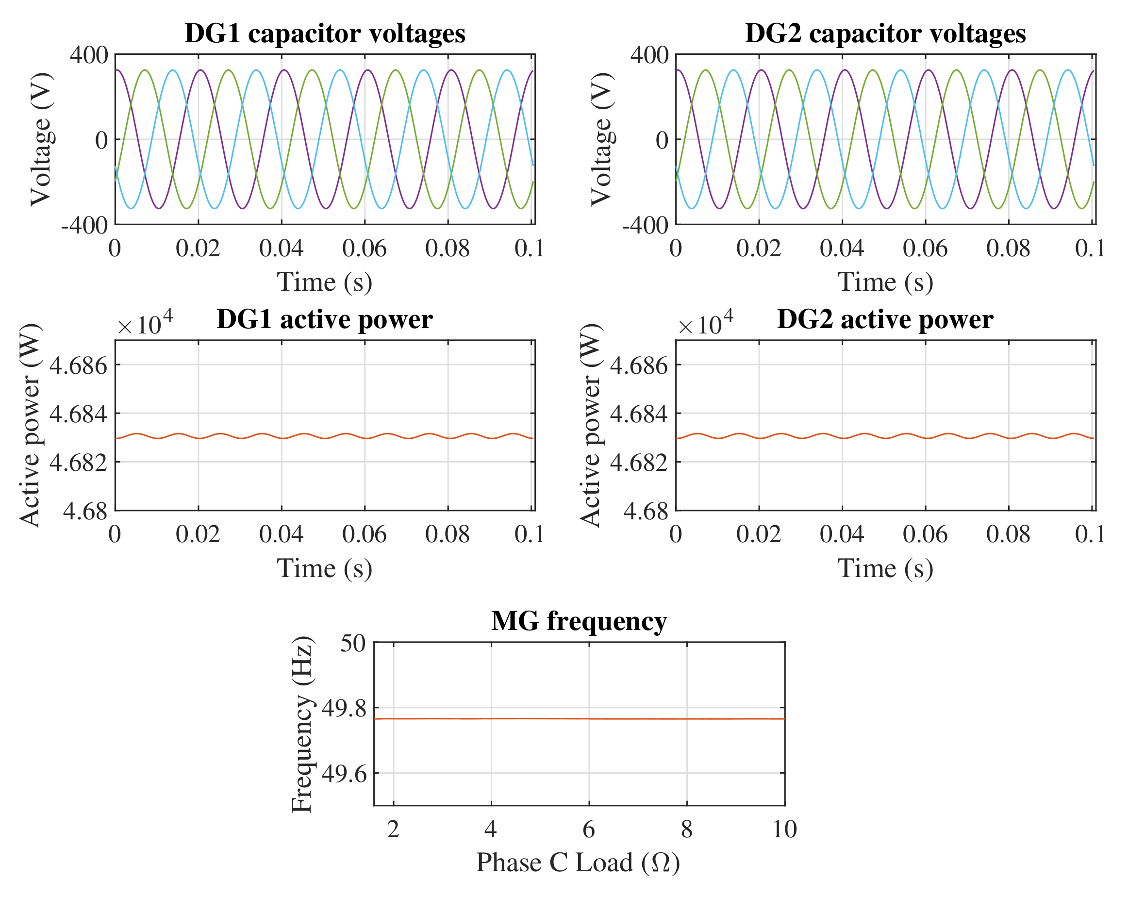
Using the obtained controlled-MG model, a time-domain simulation is performed and the results from five cycles are presented in Figure A2. In particular, the DGs controlled voltage and the active power injected by the DGs are shown. Furthermore, the system frequency during the whole phase C load variation is presented as well.
Figure A2.
Time-domain simulation of five full-cycles of the computed solution in Case 2. Additionally, the system frequency during the whole phase C load variation.
Figure A2.
Time-domain simulation of five full-cycles of the computed solution in Case 2. Additionally, the system frequency during the whole phase C load variation.

Appendix A.3. Case 2: Droop Characteristic Variation with the Converters Commutation Process Enabled
Using the obtained controlled-MG model, a time-domain simulation is performed and the results from five cycles are presented in Figure A3. In particular, the DGs controlled voltage and the active power injected by the DGs are shown. Furthermore, the system frequency during the whole variation is presented as well. It is worth mentioning that for this simulation, the initial state-vector used was the unstable solution computed via the autonomous shooting method for the Case 3.
Figure A3.
Time-domain simulation of five full-cycles of the computed unstable solution in Case 3, before the system collapses. Additionally, the system frequency during the whole variation.
Figure A3.
Time-domain simulation of five full-cycles of the computed unstable solution in Case 3, before the system collapses. Additionally, the system frequency during the whole variation.

References
- Chowdhury, S.; Crossley, P. Microgrids and Active Distribution Networks; IET Renewable Energy Series; Institution of Engineering and Technology: London, UK, 2009. [Google Scholar]
- Wan, X.; Wu, J. Distributed Hierarchical Control for Islanded Microgrids Based on Adjustable Power Consensus. Electronics 2022, 11, 324. [Google Scholar] [CrossRef]
- Khongkhachat, S.; Khomfoi, S. Hierarchical control strategies in AC microgrids. In Proceedings of the 2015 12th International Conference on Electrical Engineering/Electronics, Computer, Telecommunications and Information Technology (ECTI-CON), Hua Hin, Thailand, 24–27 June 2015; pp. 1–6. [Google Scholar] [CrossRef]
- Fotopoulou, M.; Rakopoulos, D.; Blanas, O. Day Ahead Optimal Dispatch Schedule in a Smart Grid Containing Distributed Energy Resources and Electric Vehicles. Sensors 2021, 21, 7295. [Google Scholar] [CrossRef] [PubMed]
- Rocabert, J.; Luna, A.; Blaabjerg, F.; Rodríguez, P. Control of Power Converters in AC Microgrids. IEEE Trans. Power Electron. 2012, 27, 4734–4749. [Google Scholar] [CrossRef]
- Guerrero, J.M.; Vasquez, J.C.; Matas, J.; de Vicuna, L.G.; Castilla, M. Hierarchical Control of Droop-Controlled AC and DC Microgrids: A General Approach Toward Standardization. IEEE Trans. Ind. Electron. 2011, 58, 158–172. [Google Scholar] [CrossRef]
- Yu, K.; Ai, Q.; Wang, S.; Ni, J.; Lv, T. Analysis and Optimization of Droop Controller for Microgrid System Based on Small-Signal Dynamic Model. IEEE Trans. Smart Grid 2016, 7, 695–705. [Google Scholar] [CrossRef]
- Medina, A.; Segundo, J.; Ribeiro, P.; Xu, W.; Lian, K.; Chang, G.; Dinavahi, V.; Watson, N. Harmonic Analysis in Frequency and Time Domain. IEEE Trans. Power Deliv. 2013, 28, 1813–1821. [Google Scholar] [CrossRef]
- Segundo-Ramirez, J.; Barcenas, E.; Medina, A.; Cardenas, V. Steady-State and Dynamic State-Space Model for Fast and Efficient Solution and Stability Assessment of ASDs. IEEE Trans. Ind. Electron. 2011, 58, 2836–2847. [Google Scholar] [CrossRef]
- Peña, R.; Medina, A.; Anaya-Lara, O. Steady-state Solution of Fixed-speed Wind Turbines Following Fault Conditions Through Extrapolation to the Limit Cycle. IETE J. Res. 2011, 57, 12–19. [Google Scholar] [CrossRef]
- Segundo, J.; Medina, A. Periodic Steady-State Solution of Electric Systems Including UPFCs by Extrapolation to the Limit Cycle. IEEE Trans. Power Deliv. 2008, 23, 1506–1512. [Google Scholar] [CrossRef]
- Agundis-Tinajero, G.; Segundo-Ramírez, J.; Peña-Gallardo, R.; Visairo-Cruz, N.; Núñez-Gutiérrez, C.; Guerrero, J.M.; Savaghebi, M. Harmonic Issues Assessment on PWM VSC-Based Controlled Microgrids Using Newton Methods. IEEE Trans. Smart Grid 2018, 9, 1002–1011. [Google Scholar] [CrossRef] [Green Version]
- Nayfeh, A.; Balachandran, B. Applied Nonlinear Dynamics: Analytical, Computational, and Experimental Methods; Wiley Series in Nonlinear Science; Wiley: Hoboken, NJ, USA, 2008. [Google Scholar]
- Dobson, I.; Chiang, H.D. Towards a theory of voltage collapse in electric power systems. Syst. Control. Lett. 1989, 13, 253–262. [Google Scholar] [CrossRef]
- Srivastava, K.N.; Srivastava, S.C. Elimination of dynamic bifurcation and chaos in power systems using FACTS devices. IEEE Trans. Circuits Syst. I Fundam. Theory Appl. 1998, 45, 72–78. [Google Scholar] [CrossRef]
- Wornle, F.; Harrison, D.K.; Zhou, C. Analysis of a ferroresonant circuit using bifurcation theory and continuation techniques. IEEE Trans. Power Deliv. 2005, 20, 191–196. [Google Scholar] [CrossRef]
- Segundo-Ramírez, J.; Medina, A.; Ghosh, A.; Ledwich, G. Non-linear Oscillations Assessment of the Distribution Static Compensator Operating in Voltage Control Mode. Electr. Power Components Syst. 2010, 38, 1317–1337. [Google Scholar] [CrossRef] [Green Version]
- Shuai, Z.; Hu, Y.; Peng, Y.; Tu, C.; Shen, Z.J. Dynamic Stability Analysis of Synchronverter-Dominated Microgrid Based on Bifurcation Theory. IEEE Trans. Ind. Electron. 2017, 64, 7467–7477. [Google Scholar] [CrossRef]
- Huang, S.J.; Liaw, D.C. A Bifurcation Study of Droop-Controlled Inverter-Based Microgrids with Dynamic Loads. In Proceedings of the 2021 21st International Conference on Control, Automation and Systems (ICCAS), Jeju, Korea, 12–15 October 2021; pp. 1814–1819. [Google Scholar] [CrossRef]
- Shuai, Z.; Peng, Y.; Liu, X.; Li, Z.; Guerrero, J.M.; Shen, Z.J. Parameter Stability Region Analysis of Islanded Microgrid Based on Bifurcation Theory. IEEE Trans. Smart Grid 2019, 10, 6580–6591. [Google Scholar] [CrossRef]
- Wang, Y.; Wei, F.; Zuo, Z. Modeling and Stability Analysis of DC Microgrid with Constant Power Loads. In Proceedings of the 2021 40th Chinese Control Conference (CCC), Shanghai, China, 26–28 July 2021; pp. 6799–6805. [Google Scholar] [CrossRef]
- Lenz, E.; Pagano, D.J.; Pou, J. Bifurcation Analysis of Parallel-Connected Voltage-Source Inverters With Constant Power Loads. IEEE Trans. Smart Grid 2018, 9, 5482–5493. [Google Scholar] [CrossRef]
- Jiang, X.; Li, Y.; Du, L.; Huang, D. Identifying Hopf Bifurcations of Networked Microgrids Induced by the Integration of EV Charging Stations. In Proceedings of the 2021 IEEE Transportation Electrification Conference Expo (ITEC), Chicago, IL, USA, 21–25 June 2021; pp. 690–694. [Google Scholar] [CrossRef]
- Sreeram, T.; Dheer, D.; Doolla, S.; Singh, S. Hopf bifurcation analysis in droop controlled islanded microgrids. Int. J. Electr. Power Energy Syst. 2017, 90, 208–224. [Google Scholar] [CrossRef]
- Liu, K.; Lin, L.; Tang, K.; Dong, S. Fast Calculation of Saddle-Node Bifurcation Point in Islanded Microgrid Based on Levenberg-Marquardt Algorithm. In Proceedings of the 2021 IEEE 4th International Electrical and Energy Conference (CIEEC), Wuhan, China, 28–30 May 2021; pp. 1–6. [Google Scholar] [CrossRef]
- Keyvani-Boroujeni, B.; Shahgholian, G.; Fani, B. A Distributed Secondary Control Approach for Inverter-Dominated Microgrids With Application to Avoiding Bifurcation-Triggered Instabilities. IEEE J. Emerg. Sel. Top. Power Electron. 2020, 8, 3361–3371. [Google Scholar] [CrossRef]
- Aprille, T.J.; Trick, T.N. Steady-state analysis of nonlinear circuits with periodic inputs. Proc. IEEE 1972, 60, 108–114. [Google Scholar] [CrossRef]
- Segundo-Ramírez, J.; Medina, A. Computation of the steady state solution of nonlinear power systems by extrapolation to the limit cycle using a discrete exponential expansion method. Int. J. Nonlinear Sci. Numer. Simul. 2010, 11, 655–660. [Google Scholar] [CrossRef]
- Parker, T.; Chua, L. Practical Numerical Algorithms for Chaotic Systems; Springer Science & Business Media: London, UK, 2011. [Google Scholar]
- Guerrero, J.M.; de Vicuna, L.G.; Matas, J.; Castilla, M.; Miret, J. A wireless controller to enhance dynamic performance of parallel inverters in distributed generation systems. IEEE Trans. Power Electron. 2004, 19, 1205–1213. [Google Scholar] [CrossRef]
- Agundis-Tinajero, G.; Aldana, N.L.D.; Luna, A.C.; Segundo-Ramírez, J.; Visairo-Cruz, N.; Guerrero, J.M.; Vazquez, J.C. Extended-Optimal-Power-Flow-Based Hierarchical Control for Islanded AC Microgrids. IEEE Trans. Power Electron. 2019, 34, 840–848. [Google Scholar] [CrossRef]
- Segundo-Ramirez, J.; Medina, A. Modeling of FACTS Devices Based on SPWM VSCs. IEEE Trans. Power Deliv. 2009, 24, 1815–1823. [Google Scholar] [CrossRef]
Figure 1.
Droop control block diagram.

Figure 2.
Droop control block diagram, autonomous system.

Figure 3.
Single line diagram of the test case microgrid.

Figure 4.
Comparison of the autonomous test system against the non-autonomous test system. In (a), the comparison of the DG1 output current signals for fundamental frequency is shown; in (b), the comparison of the DG1 output current signals for the commutated model is shown; and in (c), the comparison of the active power injected to the load for the commutated case is shown.

Figure 5.
Floquet multipliers result from the variation , .

Figure 6.
Phase portrait between DG1 currents phase A and B. Neimark–Sacker supercritical bifurcation forming a torus attractor.
Figure 6.
Phase portrait between DG1 currents phase A and B. Neimark–Sacker supercritical bifurcation forming a torus attractor.

Figure 7.
Stability boundary map with and as bifurcation variables (Dark blue stable, otherwise unstable).
Figure 7.
Stability boundary map with and as bifurcation variables (Dark blue stable, otherwise unstable).

Figure 8.
Floquet multipliers result from the variation .

Figure 9.
Floquet multipliers and system frequency result from the variation , ].

Figure 10.
Phase portrait between DG1 currents phase A and B. Neimark–Sacker supercritical bifurcation forming a torus attractor.
Figure 10.
Phase portrait between DG1 currents phase A and B. Neimark–Sacker supercritical bifurcation forming a torus attractor.


Table 1.
Parameters of the case study microgrid and control.
| Parameter | Symbol | Value |
|---|---|---|
| Nominal voltage | 400 V | |
| Nominal frequency | 50 Hz | |
| Nominal DC voltage | 1500 V | |
| Filter resistance | 0.1 | |
| Filter inductance | 1.8 mH | |
| Filter capacitance | 27 F | |
| Feeder resistance | 0.1 | |
| Feeder inductance | 1.8 mH | |
| droop coefficient | 3 | |
| droop coefficient | 4 | |
| Voltage loop proportional gain | 20 | |
| Voltage loop integral gain | 50 | |
| Current loop proportional gain | 2.4 | |
| Current loop integral gain | 4.5545 | |
| Frec. rest. proportional gain | 0.02 | |
| Frec. rest. integral gain | 4 | |
| Voltage rest. proportional gain | 0.2 | |
| Voltage rest. integral gain | 4 | |
| Switching frequency | 10 kHz |
Publisher’s Note: MDPI stays neutral with regard to jurisdictional claims in published maps and institutional affiliations. |
© 2022 by the authors. Licensee MDPI, Basel, Switzerland. This article is an open access article distributed under the terms and conditions of the Creative Commons Attribution (CC BY) license (https://creativecommons.org/licenses/by/4.0/).
Share and Cite
MDPI and ACS Style
Agundis-Tinajero, G.D.; C. Vasquez, J.; Guerrero, J.M. Stability Boundary Analysis of Islanded Droop-Based Microgrids Using an Autonomous Shooting Method. Energies 2022, 15, 2120. https://doi.org/10.3390/en15062120
AMA Style
Agundis-Tinajero GD, C. Vasquez J, Guerrero JM. Stability Boundary Analysis of Islanded Droop-Based Microgrids Using an Autonomous Shooting Method. Energies. 2022; 15(6):2120. https://doi.org/10.3390/en15062120
Chicago/Turabian StyleAgundis-Tinajero, Gibran D., Juan C. Vasquez, and Josep M. Guerrero. 2022. "Stability Boundary Analysis of Islanded Droop-Based Microgrids Using an Autonomous Shooting Method" Energies 15, no. 6: 2120. https://doi.org/10.3390/en15062120
Note that from the first issue of 2016, this journal uses article numbers instead of page numbers. See further details here.