Article

Efficiency Increase through Model Predictive Thermal Control of Electric Vehicle Powertrains

1
Teaching and Research Area Mechatronics in Mobile Propulsion, Faculty of Mechanical Engineering, RWTH Aachen University, Forckenbeckstraße 4, 52074 Aachen, Germany
2
Chair of Thermodynamics of Mobile Energy Conversion Systems, Faculty of Mechanical Engineering, RWTH Aachen University, Forckenbeckstraße 4, 52074 Aachen, Germany
3
FEV Europe GmbH, Neuenhofstr. 181, 52078 Aachen, Germany
*
Author to whom correspondence should be addressed.
Energies 2022, 15(4), 1476; https://doi.org/10.3390/en15041476
Submission received: 2 February 2022 / Revised: 10 February 2022 / Accepted: 15 February 2022 / Published: 17 February 2022

Abstract

:
Battery electric vehicles (BEVs) are currently enjoying rising sales figures. However, BEVs still have problems with customer acceptance, partly due to limited driving ranges. To improve the situation, this paper introduces a novel approach utilising temperature-dependent efficiencies using an economic model predictive control approach (MPC) in combination with an active grille shutter in order to accelerate the heating of the permanent magnet synchronous machine. The measurements of temperature-dependent component efficiencies on a powertrain test bench are presented and analysed in detail in the speed/torque range. Thermal models based on the lumped parameter thermal network approach were developed and validated as part of the system-level validation against a US06 wind tunnel measurement. After the build-up and implementation of the MPC, various simulations were conducted. For the investigations, three driving cycles were considered at component start temperatures of 20–80 °C. The results show that using the MPC with the grille shutter can save 0.69–2.02% energy at the HV level compared to the rule-based control with a shutter, of which up to 1.02% is due to temperature-dependent efficiencies. Comparing the MPC with the grille shutter to a vehicle without a shutter, savings of 2.8–4.2% were achieved, while up to 1.67% was achieved due to temperature effects in the powertrain.

1. Introduction

In recent years, the sales of battery electric vehicles (BEVs) have continuously grown, reaching 1.5 million sales globally in 2019, with a total market share of around 1% [1]. The intention to buy a BEV seems to be quite high. It ranged from 16% in the United States to 45% in Japan in 2021 [2]. However, many consumers still have concerns, especially regarding the battery charging infrastructure and times as well as the driving range [2,3]. Studies such as [4] show that the boundary conditions, especially regarding the charging infrastructure, are uneven between countries even within Europe. While [5] highlights a lack of charging infrastructure in the Górnośląsko-Zagłębiowska Metropolis in Poland as one reason for the low BEV sales in the country, the study in China presented in [6] concluded that experiencing electric mobility enhances the willingness to buy an electric vehicle.
On the vehicle side, approaches such as reliable range prediction and fast charging are being researched to improve customer acceptance [3,7,8]. Amongst others, these aspects are being addressed by the CEVOLVER project [9], which targets a higher long-distance travel capability of BEVs, reducing the battery size to minimise hardware costs and also mitigating the environmental impact of battery production. The trade-off between the battery size, trip time, and charging power was already analysed in [10]. Another aspect that enhances the long-distance travelling capability is reducing the power demand of the vehicle and thus increasing the range per battery charge. As intelligent control strategies have been proven to be an efficient way to increase the energy efficiency of various vehicle types, this aspect is the focus of this contribution.
Optimal control of thermal systems using model predictive control (MPC) has been a topic of intensive research since the 1990s in the field of climate control in buildings [11]. Novel approaches in this domain utilise predictive data such as weather forecasts, as was considered in [12,13,14]. In recent years, thermal vehicle management, especially in BEV applications, has received more and more attention. In extreme conditions, the driving range can be reduced by up to 60%, especially due to the heating of the cabin in winter conditions [15,16,17,18]. Thus, several publications have shown how control strategies combined with hardware measures, especially heat pumps, can lead to significant improvements. Around an 11% reduction in energy consumption for a New European Driving Cycle (NEDC) at −10 °C was achieved in [19] using an artificial neuronal network (ANN) in combination with optimisation steps. In contrast, in [20], energy savings of 34% at a 10 °C ambient temperature and around 8% at −10 °C were shown using a rule-based strategy optimised with a parameter variation. Next to cabin heating, the battery was also a focus of interest, with the main emphasis on ageing as well as energy savings. In [21], a two-layer MPC was used to improve the efficiency by 3–8% depending on the boundary conditions. The energy efficiency of the battery thermal control was optimised for a BEV by a stochastic model predictive control (SMPC) approach in [22]. In [23], energy savings of up to 5% for a custom driving cycle were achieved using an MPC for a plug-in hybrid electric vehicle (PHEV).
Powertrain energy management on a system level towards temperature-dependent efficiencies has been a focus of interest for hybrid electric vehicles (HEVs) and internal combustion engine (ICE) applications already. In [24], a 2% fuel consumption advantage was achieved for a vehicle with an ICE powertrain by reducing the friction and power demand of the auxiliaries for an urban dynamometer driving schedule (UDDS) cycle with a dual-mode coolant pump that can run in mechanical and electrical modes in combination with a rule-based controller. Additionally in [25], a comparison of a mechanical/electrical coolant pump combined with a continuous/switching valve using model predictive control for an ICE powertrain was evaluated. The main outcome was a saving of 2% for the EPA Federal Test Procedure (FTP75) and 1% for the US06 cycle by increasing the oil and engine metal temperature, which led to friction reduction. In [26], an MPC was used to minimize the fuel consumption of an ICE vehicle considering the engine metal and oil temperature with regard to fuel efficiency. On the other hand, in [27], an optimisation-based strategy for cabin climatisation, engine, and exhaust gas aftertreatment of an HEV was presented, which showed fuel savings of 10–26% for a real-world cycle and the UDDS cycle by optimising the heat harvesting from the ICE to heat the cabin. An electric powertrain can also be used as a heat source for a heat pump system, as shown in [28] for an HEV. In combination with waste heat recovery from the exhaust gas after treatment, fuel savings of up to 13.1% were achieved in the NEDC driving mode.
The contributions of this paper are as follows:
  • Energy management through economic model predictive thermal control for BEV application;
  • Controlling the temperature of the motor and inverter to utilise temperature-dependent efficiencies, especially by closing the shutter for faster heating;
  • Reduced pump and fan power draw, as well as decreased shutter-based drag force by optimal control;
  • Detailed controller-oriented modelling of the vehicle and thermal system, as well as the motor and inverter, including system-level validation;
The paper is structured as follows: First, in Section 2, an overview of the hardware setup is presented, followed by Section 3, which provides an introduction to the MPC approach and the problem formulation. Then, the temperature-dependent efficiencies for the electric machine and inverter are described in detail in Section 4, followed by the system modelling and the system level validation in Section 5. The results of the comparison between the MPC controller and the rule-based approach are described in Section 6. Finally, Section 7 concludes the paper.

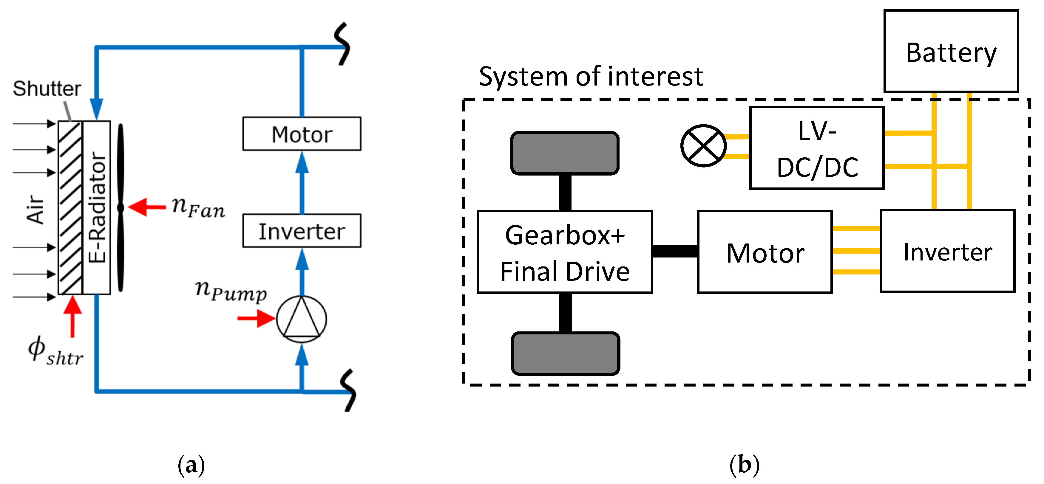
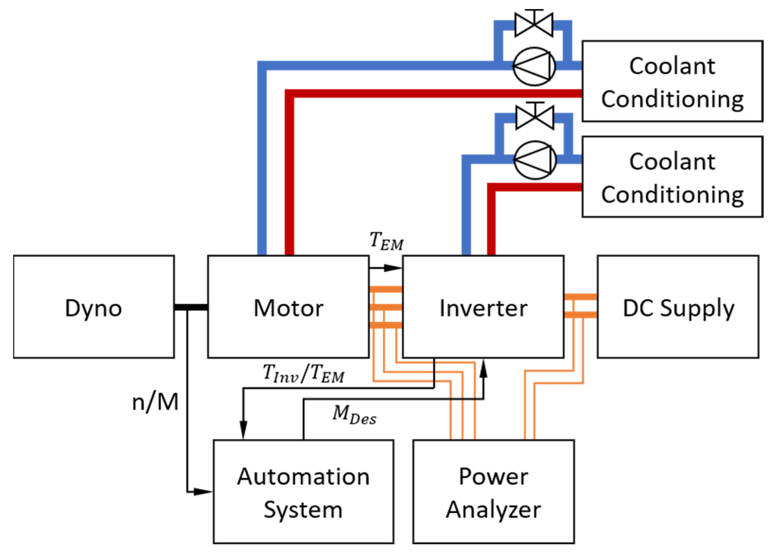
2. Overview of the Setup

The vehicle that was used for the investigations was a Fiat 500, which was converted from a combustion engine vehicle to a BEV in the Smart Wheels Project [29] and then rebuilt with new powertrain and thermal components. Neither the vehicle nor the measurements throughout this paper were built or obtained within the CEVOLVER project. The parameters used for a physics-based vehicle model, which were already partly presented in [30], are summarized in Table 1. The gross weight of the vehicle was 1335 kg, including the driver and battery. As is typical for most electric vehicles, it had a fixed gear ratio. The drag coefficient was measured in a wind tunnel.
The thermal hardware layout is depicted in Figure 1a. It consists of a coolant pump, an inverter, an electric machine motor, and a radiator. A 50/50 water–glycol mixture was used as a cooling fluid. The motor was cooled by a water jacket, while the inverter was cooled using a cooling plate. The coolant was circulated by a Pierburg CWA100 pump, which has a rated electrical power of 100 W [31]. A fan located behind the radiator was used to increase the air volume flow. The depicted shutter was considered only for the simulation. In Figure 1a, the control variables are marked separately with red arrows to highlight the degrees of freedom. The fan was controlled using the rotational speed signal n F a n , while the pump received the rotational speed signal n P u m p as a set point. The shutter position was controlled with the continuous opening signal ϕ s h t r .
The powertrain and the electrical topology are depicted in Figure 1b. The layout consists of a DC high-voltage lithium-ion battery, a low-voltage DC/DC converter (LV-DC/DC), as well as an inverter. For the inverter, a Brusa DMC 524 was used, which has a voltage range of 120–450 V, with a maximum power of 105 kW and a rated efficiency of 97% [32]. The vehicle used an interior permanent magnet synchronous motor (IPMSM) of the Brusa HSM1-6.17.12 type with three pole pairs. It deliveres a continuous torque of 130 Nm and a peak torque of 220 Nm [33]. The maximum speed was 12,000 rpm and the motor has a rated efficiency of 95%. The gearbox and the final drive are air cooled. The system of interest in this study is highlighted in the figure by the dashed box.

3. Model Predictive Control as a Method for Controlling Temperatures of the Powertrain

Control methods that use a system model to predict process variables and calculate a control variable trajectory are known as model predictive control (MPC). An MPC uses the current states of the system and predictive data to optimise the future states and controls based on a scalar cost function. When formulating the optimisation problem, constraints can be directly included, for example, with the Lagrange function. This is an advantage of the MPC approach in contrast to indirect methods, which are based on Pontryagin’s minimum principle [34,35]. In MPCs with reference tracking, the deviation of the state variables from a given reference trajectory is minimized by a cost function. In contrast, the cost function of an economic MPC has no reference trajectory and is composed solely of economic cost terms, such as energy consumption [36].
The cost function J in (1) for the economic MPC of this contribution describes the power losses and electrical consumption of the components considered. This includes the power loss of the electric motor P E M , L o s s and the inverter P I n v , L o s s , the electrical power demands of the coolant pump P e l , P u m p and the fan P e l , F a n . For the low-voltage (LV) actuator supply, a constant electrical DCDC efficiency of η D C D C = 0.9 was considered. When the grille shutter is closed, the cost function value is reduced by P S h u t t e r , which describes the reduced power demand by lowering the drag coefficient c d . Due to the low energy consumption, the electrical power demand of the grille shutter motor was neglected.
J = P E M , L o s s + P I n v , L o s s P S h u t t e r + P e l , P u m p + P e l , F a n η D C D C
y = [ P E M , L o s s , P I n v , L o s s , P S h u t t e r , P e l , P u m p , P e l , F a n ] T = f ( x , u , n E M , M E M )
x ˙ = f ( x , u , t )
x = [ T E M , T I n v ,   T C o E , T C o I , T C o R ] T
u = [ n P u m p , n F a n , ϕ s h t r ] T
The considered system model is described by (2)–(5), starting with the system output vector y . The instances of the letter “T” at the right side of the brackets in (2), (4), and (5) indicate that the content is transposed from a column vector to a row vector. The outputs are the above-described powers, which are dependent on the states x , the controls u , as well as the motor speed n E M and the torque M E M . The states are described in (4), which are solely the temperatures of the motor T E M , the inverter T I n v as well as the coolant temperature downstream of the motor T C o E , inverter T C o I , and radiator T C o R . The controls in (5), which are highlighted in Figure 1a, are the speed of the coolant pump n P u m p and the fan n F a n , as well as the grille shutter position ϕ s h t r . The system model, which was integrated using an implicit Runge–Kutta second-order method, is described in (3) [37]. Here, x ˙ is the time derivative of the state x , and t is the time in the continuous domain [34,35].
In (6), the constraints on the temperature states x i of the thermal system are defined. All temperature limits were set to their respective values taken from the data sheets. For the water–glycol coolant, the limits were set according to the evaporation and solidification temperature with a safety reserve at these temperatures. The limits of the controls u i in (7) were set according to the physical limitations of the real components.
x m i n , i x i x m a x , i ,   i = 1 , , 5
u m i n , i u i u m a x , i ,   i = 1 , , 3
The high-performance software package acados was used to set up and solve the non-linear-problem (NLP) [38]. acados contains algorithms by which the cost function, the system equations, and the constraints can be transformed into an NLP. The optimisation problem, which was discretized using the multiple-shooting method, was solved using the sequential quadratic programming method (SQP). In SQP, the discretized Lagrangian function containing the cost function and the constraints was quadratically approximated using a Taylor series. The resulting quadratic problem was solved using the gradient-based interior-point solver HPIPM, which is based on the linear algebra software framework BLASFEO [39,40]. Furthermore, regularization methods integrated into acados were applied to ensure a positive definite Hessian matrix [41]. In order to stabilize the MPC against a temperature limit violation, soft constraints were added as quadratic costs that penalized the distance to the constraint when exceeded.

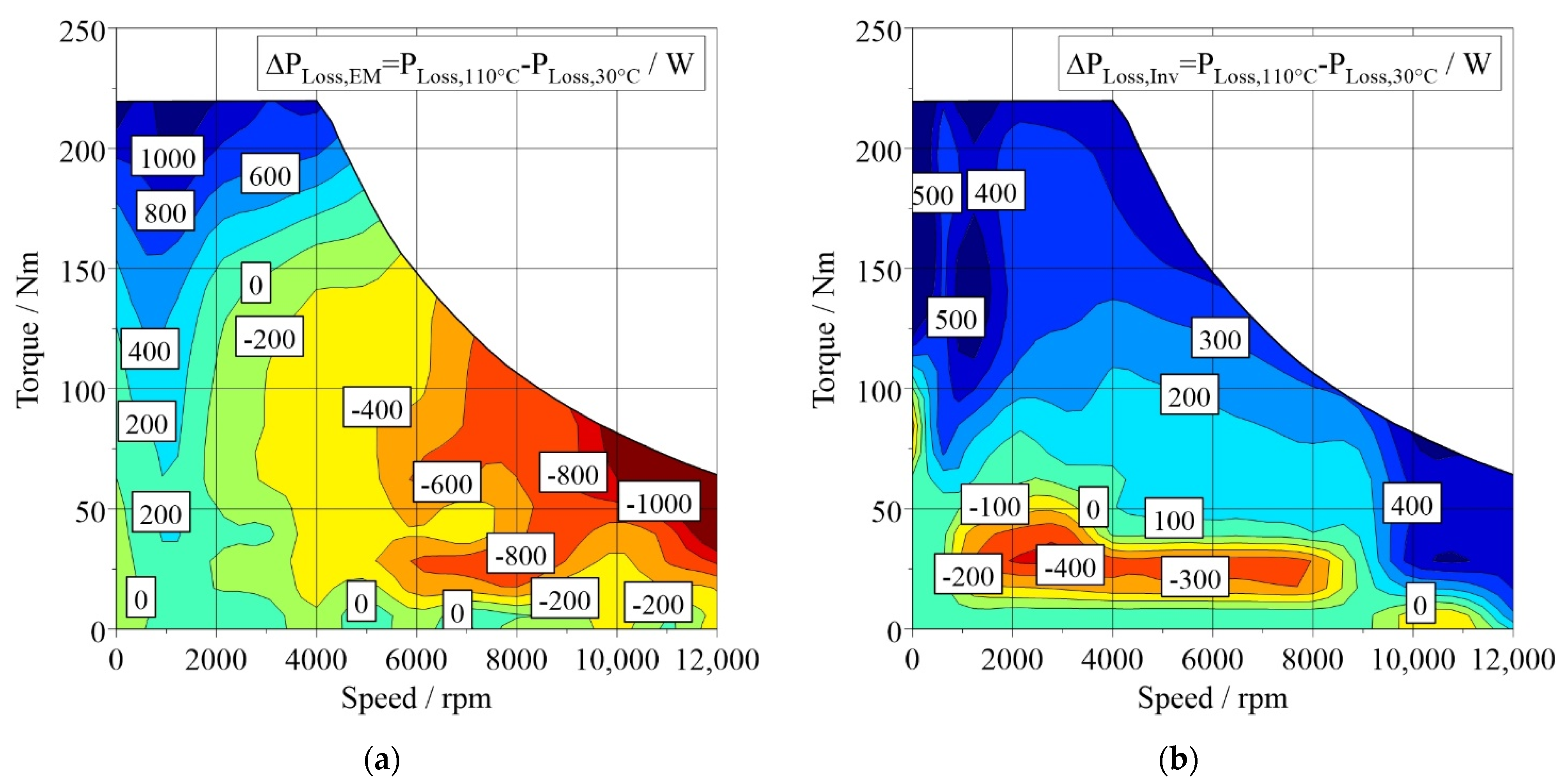
4. Discussion of Temperature-Dependent Electrical Efficiencies of Motor and Inverter

In this section, the temperature-dependent efficiencies are explained in the speed/torque domain after introducing the measurement setup. For both components, the inverter and electric machine, the losses were measured on a test bench in the whole speed/torque map at different temperatures and DC voltages. The measurement setup, which was already shown in [30], is depicted in Figure 2, showing the motor and inverter on a test bench. The DC supply controlled the voltages at the input of the inverter to 300 V, 350 V, and 400 V, while the conditioning systems controlled the temperatures of the motor and inverter using the internal measurements from the NTC sensors of the inverter. Each operating point was measured at temperatures of −10 °C, 30 °C, 70 °C, and 110 °C within a range of +/−3 °C. In order to obtain the efficiencies, a speed/torque measurement at the shaft flange was used, as well as the power draw at the inverter input and output [30].

4.1. Temperature-Dependent Motor Losses

Figure 3a shows the changes in the motor power losses when the temperature increased from 30 °C to 110 °C at a constant battery voltage of 400 V. Negative values represent a loss reduction at higher temperatures. When the temperature increases in low load operations at medium to high speeds, such as during constant highway driving, there is a potential of up to 1.3 kW in the sweet spot considering the motor loss. Nevertheless, higher temperatures are not beneficial for high load operations at low speeds, leading to loss increases of up to 1.2 kW.
These observations can be explained considering the motor loss mechanisms. In a PMSM, the total losses P L o s s , T o t , P M S M can be divided into copper P L o s s , C o p p e r , iron P L o s s , I r o n , magnet P L o s s , M a g n e t , and mechanical losses P L o s s , M e c h :
P L o s s , T o t , P M S M = P L o s s , C o p p e r + P L o s s , I r o n + P L o s s , M a g n e t + P L o s s , M e c h
For all loss mechanisms, excluding the mechanical loss, the specific electrical resistance ρ ( T ) as a function of temperature is relevant [42]:
ρ ( T ) = ρ 0 · [ 1 + α · ( T T 0 ) ]
At a certain temperature T , it can be calculated by the specific initial resistivity ρ 0 at temperature T 0 and the temperature coefficient α , which is positive for metals such as copper and iron. The first motor loss mechanism P L o s s , c o p p e r is the most significant at high motor torques, as the current in the copper windings rises and the losses increase with respect to the temperature-dependent phase resistance [42,43]:
P L o s s , C o p p e r = i 2 · ρ C u ( T ) · l A = i 2 · ρ 0 · [ 1 + α · ( T T 0 ) ] · l A
The copper loss is calculated by the specific electrical resistance ρ C u ( T ) , the length l , and the cross-section A of the conductor, as well as the current i . According to (10), it increases proportionally with the temperature.
Second, the temperature dependence of the iron losses P L o s s , I r o n can be evaluated by splitting it into two main loss mechanisms, the Eddy P L o s s , E d d y   and Hysteresis Losses P L o s s , H y s t [44]:
P L o s s , I r o n = P L o s s , E d d y + P L o s s , H y s t
Due to the frequent change in the magnetic flux density, a voltage is induced inside the stator and rotor laminations, which leads to eddy currents [45]. Eddy current losses are derived from Maxwell’s law [46]:
P L o s s , E d d y = π 2 6 1 ρ F e d 2 f 2 B ^ 2
In (12), the eddy current losses are derived from the specific electric resistance ρ F e and the diameter d of the metal sheets, as well as the frequency f and amplitude of the magnetic flux density B ^ . Under consideration of (9), eddy currents are inversely proportional to temperature and quadratically proportional to frequency. This explains the higher efficiency at increased temperatures in the field-weakening range in Figure 3a.
The specific hysteresis losses P L o s s , H y s t are defined by the space inside the hysteresis loop of magnetisation, which results from the material behaviour. Because of a decreasing saturation polarisation for the laminations with increasing temperatures, the hysteresis losses can also be reduced by an increased temperature of the PMSM [43].
Likewise, the loss mechanism P L o s s , M a g n e t in permanent magnets is due to eddy currents that heat the magnets [43]. Consequently, the remanence flux density of the permanently excited rotor is reduced by these higher temperatures, which also decreases the maximum possible torque [47,48]. However, the amount of required negative d-current in the field-weakening area is reduced as well. The lower flux density B ^ at increased magnet temperatures additionally lowers the iron losses, as can be seen in (12). The mechanical losses P L o s s , M e c h in the PMSM are mainly dependent on the rotational speed, as they are related to friction losses in the bearings and windage losses in the airgap between the stator and rotor. While the viscosity of the oil in the bearings decreases with higher temperatures, the viscosity of the air in the airgap increases. However, both loss mechanisms are several orders smaller than the electromagnetic losses described before, so they can be neglected considering Figure 3a [44].

4.2. Temperature-Dependent Inverter Losses

The main loss sources in inverter operations are the insulated gate bipolar transistors (IGBTs) [49] as well as the copper losses in the cables. The overall inverter losses are approximated by P L o s s , T o t , I n v :
P L o s s , T o t , I n v = P L o s s , S w i t c h + P L o s s , C o n d + P L o s s , C o p p e r
The IGBTs introduce heat to the inverter by switching losses P L o s s , s w i t c h , which are dominant at high frequencies, as well as conduction losses P L o s s , C o n d [49]. Furthermore, the copper losses in cables   P L o s s , C o p p e r , which were described by (10), are relevant. While the switching losses proportionally increase with rising temperatures due to a change in the collector current slopes during a switch event, as described in [50] and [51], the conduction losses have a changing NTC to PTC behaviour with an increasing current injection [51,52]. Thus, in low load operations, respectively at low current injections, the conduction losses decrease with increasing temperatures, due to the NTC behaviour. This can be seen in Figure 3b for a small area under 50 Nm, as the conduction loss NTC behaviour dominates over the copper and switching losses. The maximum loss reduction for high temperatures is about 400 W. At higher loads and higher current injections, the PTC behaviour of P L o s s , C o n d as well as the PTC behaviour of the copper and the switching losses are the loss terms most relevant. This leads to increasing losses at higher temperatures around a maximum difference of 1 kW for high torques. As switching losses increase with higher frequencies, they become dominant over the conduction losses at high speeds. Therefore, the benefit of an increased temperature at higher speeds diminishes and is eventually lost, as can be seen in Figure 3b for speeds above 9000 rpm [51].

5. System Modelling and Validation

In this section, the model of the system and the electrical components are presented. First, the thermal and electrical modelling of the motor and inverter are described. Then, the thermal system components are presented. After the shutter modelling section, the system validation is shown.

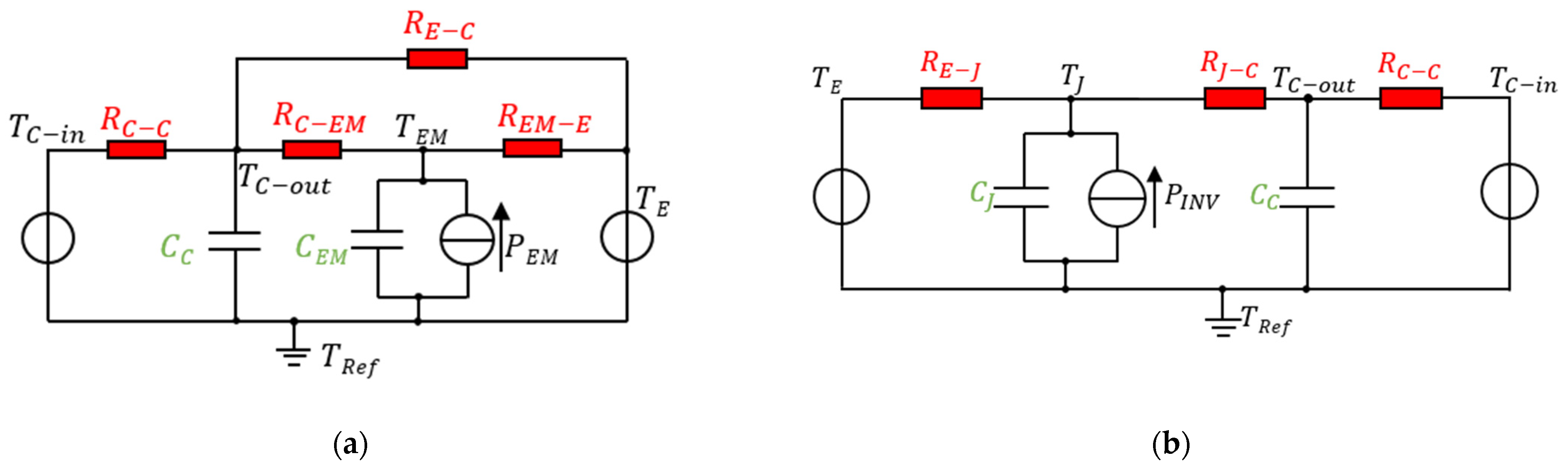
5.1. Thermal and Electrical Modelling of Motor and Inverter

The lumped parameter thermal network (LPTN) modelling approach for thermal modelling of the electrical components for determining the relevant component temperatures was applied as shown in [53,54]. In LPTN models, heat transfer processes are abstracted by equivalent electric circuit diagrams [55,56]. The analogy of the electrical current I and heat flow Q ˙ was used, as shown in the following equation:
Δ T = R T h e r m · Q ˙   U = R E l   · I
Parts of a component with similar temperatures are lumped together as a single node in the network, which is separated from other nodes by thermal resistances to represent the heat transfer between different parts [57]. The proposed LPTN models for the electric motor and inverter in this contribution are shown in Figure 4.
The high abstraction level of the LPTNs in Figure 4 enables a low computing effort, which is beneficial for model predictive control. Only two temperature nodes are used for the electric motor, representing the average motor temperature T E M and the coolant outlet temperature   T C o u t . Similarly, the nodes T J and T C o u t represent the junction temperature of the inverter and the coolant outlet temperature, respectively.
The coolant inlet temperature T C i n and the environment temperature T E are used as boundary conditions for the thermal systems. They are depicted as temperature sources. Furthermore, the losses P i are introduced as heat sources. In addition, the capacitances C i represent the thermal masses, which are defined by the gravitational mass and the specific heat capacity. Finally, the resistances R i j represent the thermal resistance, which hinders the heat flow from one component i to another component j .
When summarizing the LPTN system equations, the general state-space representation can be derived [34,37].
x ˙ = A x + B u y = C x + D u
The exact state space matrices   A ,   B ,   C , and D , as well as the state vector x and the input vector u are used to calculate the output vector y and the time derivative x ˙ . Although the system formulation derived from the LPTNs is linear, the usage of nonlinear resistances (16) results in a nonlinear system. The convective heat transfer, representing the laminar and turbulent coolant or air flow, is modelled as in [58] as a function of the fluid flow rate V ˙ and the fluid temperature T :
R i j = R t h , r e f · ( V ˙ r e f V ˙ ) b t h α t h · ( 1 T r e f T ) · ( T r e f T ) a t h
The factors α t h , a t h , and b t h are fitting coefficients determined in the identification process, while R t h , r e f , V ˙ r e f , and T r e f are reference values for the thermal resistance, volume flow, and temperature, respectively. The resistances R C C ,   R J C ,   R J E ,   and R C E M are modelled according to (16). As the housing of the motor is modelled indirectly, R E C uses (16) twice. The equations are multiplied, once for the air flow and once for the coolant flow. On the other hand, R E M E represents the heat conduction through the shaft to the gearbox, which is assumed to have an ambient temperature. Therefore, it is modelled as a constant [55]. Due to the sensitive temperature dependency of IGBT materials, the junction temperature is taken into account for modelling the capacity C J and it is modelled as in [59]. All other capacitances are assumed to be constant.
Finally, for the electrical modelling, temperature-dependent loss maps were used to create polynomials of the fourth order as a function of speed and of second order as a function of torque using the MATLAB curve fitting toolbox [60]. For the model of the plant and the controller, temperatures of 30 °C and 110 °C were considered at 400 V. In the plant model, values outside of this range were clipped.

5.2. Modelling of Thermal System Components

The modelling of the thermal system components, including the pump, fan, radiator, and shutter, is explained in the electrical as well as the fluid mechanical domain. For modelling, the pump speed was correlated to the volume flow as well as the power draw with a second-order polynomial dependency. The dynamic behaviour was considered with a first-order lag element. The fan model was map-based and combined with a first-order lag element as well. The air velocity through the radiator was correlated by polynomials of the third order regarding the vehicle velocity and of the first order regarding the fan speed. The data were measured at a wind tunnel roller dyno test bench.
The radiator was modelled by using the ϵ -NTU Theorem for crossflow heat exchangers according to [61,62]. It defines the effectiveness ϵ to calculate the transferred heat Q ˙ between the two fluid flows from the maximum possible one Q ˙ m a x [27]:
  Q ˙ = ε Q ˙ m a x
T c o o l a n t , o u t = T c o o l a n t , i n ϵ Q ˙ m a x C ˙ c o o l a n t
The effectiveness ϵ for crossflow heat exchangers can be found in [61] and [63]. It is calculated based on the dimensionless quantity of the number of transfer units (NTUs), which characterizes the size of the radiator. In (18), the radiator coolant outlet temperature is shown, which is required for the system model. It is obtained by an energy balance around the fluid in the radiator with Q ˙ from (17) as a heat source considering the inlet temperature T c o o l a n t , i n and the heat capacity flow C ˙ c o o l a n t . The steady-state coolant outlet temperature T c o o l a n t , o u t was super positioned with a first-order lag element.

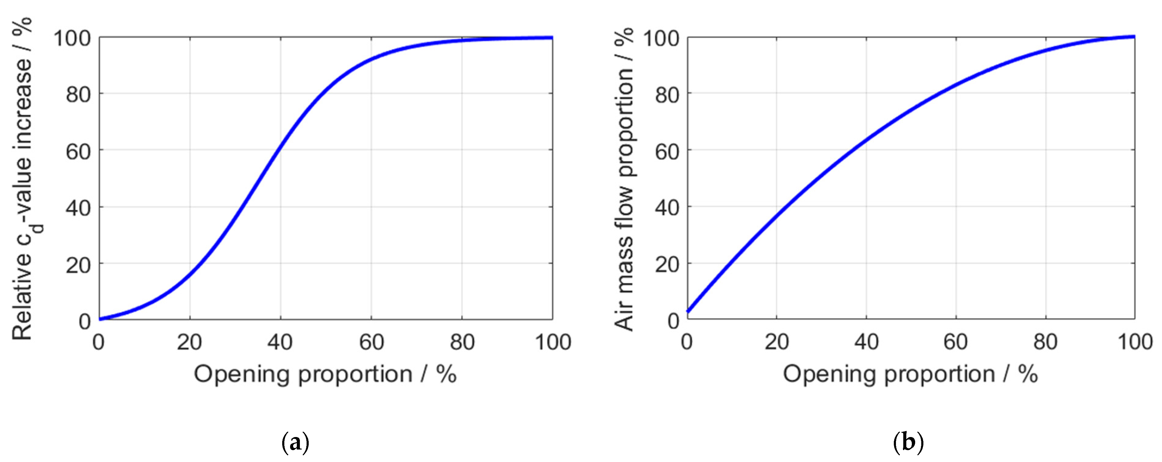
5.3. Active Grille Shutter (AGS)

In this contribution, the potential of an active grille shutter was investigated as an additional degree of freedom regarding cooling, as well as a measure to reduce the vehicle’s air drag. The vehicle was modelled using physics-based equations as a forward simulation model with a PID-based driver model. The basic correlation in order to obtain the motor speed and torque is given in the following equation [64]:
  F W h l = F A i r + F R o l l + F S l o p e + F A c c e l
In (19), the total driving force F W h l at the wheel level is calculated as the superposition of the air drag resistance F A i r , the rolling resistance F R o l l , the slope resistance F S l o p e , and the acceleration resistance F A c c e l . As the air resistance force is of special interest for the shutter actuation, the equation is shown in detail in [64], as follows:
F A i r = c d ( ϕ s h t r ) A ρ Air v r e l 2 2
The air drag force F A i r is calculated using the front area of the vehicle A , the air density ρ A i r , and the relative air velocity v r e l , which is a superposition of the vehicle speed and the wind speed. Furthermore, the drag coefficient c W ( ϕ s h t r )   is used, which in contrast to [64] in this paper is dependent on the shutter position ϕ s h t r . Closing the latter reduces the coefficient, leading to a decreased driving resistance.
Using an AGS, the air volume flow through the coolant radiator and by this, the heat dissipation can be actively controlled, influencing the coolant and the temperatures of the components [65,66,67]. Furthermore, closing the AGS decreases the c d -value up to 5.1% [65,68,69,70,71,72,73,74]. The control of the AGS has been studied in detail for vehicles with internal combustion engines in the past for fuel savings by lowering the air resistance and engine friction while not exceeding the maximum temperature for safe engine operation [66,68,75]. The influence of the shutter position was modelled in this work by approximating the CFD-based and experiment-based curves from [66,69,76,77]. Wolf [69] defined a function to correlate the opening angle with the opening proportion for rotatory AGS flaps depending on the number of flaps per air duct and the relative rotation direction to each other. This correlation was used to calculate the opening proportions when possible; otherwise, a linear relationship was assumed.
The relative change in the experimentally determined c d -values is shown in Figure 5a. It has a sigmoidal shape. The latter can be modelled using a logistic function, which is also commonly used in neural networks [78]. Equation (21) shows the modelled function of the drag coefficient c d ( ϕ s h t r )   as a function of the opening proportion of the AGS ϕ s h t r and the constants K s h t r , c w , i (i = 1,…,4).
c d ( ϕ s h t r ) = Δ c d ( K s h t r , c w , 1 1 + e ϕ s h t r K s h t r , c w , 2 + K s h t r , c w , 3 + K s h t r , c w , 4 ) + c d , S h t r , c l o s e d
The base drag coefficient is represented by c d , S h t r , c l o s e d , whereas the drag increase by opening the shutter is considered in Δ c d . The air mass flow rate curve was approximated quadratically, as shown in Figure 5b on the right side. Wind forces and construction-related gaps can cause air to flow through the AGS even when it is closed [65,66,69,79]. In this contribution, a design according to Pfeifer [65] was used, which had an air leakage of 2.5% and was approximately speed-independent. In the same contribution, the air resistance depending on the longitudinal position of the AGS was investigated in a wind tunnel. The best savings were achieved with the AGS in the far front. For consistency, the drag coefficient reduction of 4.7% from [65] was used in the simulation.

5.4. System-Level Model Validation

After describing the model design and the fitting of the components in detail, the validation is shown at a system level. The component models were parametrized using the worldwide harmonized light vehicles test cycle (WLTC) at 20 °C and 35 °C. As the component level validation already showed good results, a system-level validation was done. This was more challenging, as the components influenced each other. Moreover, two consecutive US06 driving cycles at 20 °C measured on a roller dyno were used for the validation, which contained operation points that were not part of the fitting to the WLTCs. The system layout shown in Figure 1a indicates a residual thermal system. The state of the coolant mixing with the coolant from the powertrain branch was known from measurements. For the system validation, this was considered an imposed boundary condition assuming ideal mixing before entering the radiator. The vehicle velocity and the temperatures within the system are depicted in Figure 6 within the time domain.
Next to the velocity, Figure 6 depicts the junction temperature T J measured and simulated using the LPTNs from Figure 4b. This temperature correlated very well with the torque output of the motor as the current increased. Because the thermal mass of the junction was small, high frequencies in the temperature signal occurred. In contrast, the time constants of the other thermal masses were much higher, which led to a stiff problem. In order to reduce the stiffness of the problem for longer possible integration intervals, the thermal mass of the junction was increased. As a result, the simulated temperature traces tended to follow the average temperature, as seen in Figure 6. This resulted in high maximum deviations of up to 10.97 °C, but a low RMSE.
Below the inverter temperature in Figure 6, the motor temperature T E M is depicted. It can be seen that the highest overall temperature rise within the system occurred with the motor starting at 20 °C and ending around 70 °C. Peak deviations of up to 9.66 °C and an RMSE of 3.81 °C can be seen, as the temperature estimation was constantly too low. Because the deviations need to be considered in the context of the high temperature rise, the fitting is considered sufficient, also because the tendencies of the temperature traces are matched well. Next to the motor and inverter temperatures, the coolant outlet temperatures of the radiator T C o R , the electric motor T C o E , and the inverter T C o I are depicted. Generally, considering a maximum RMSE of 0.56 °C and a maximum deviation of 1.69 °C throughout all coolant temperatures, the fitting is considered to be good.

6. Simulation Results: Efficiency Increase Using Model Predictive Control

In this section, the comparisons of the MPC approach with the rule-based baseline with and without shutter are made. First, the considered driving cycles, as well as the rule-based baseline strategy, are presented. Then, the different control approaches are compared energetically.

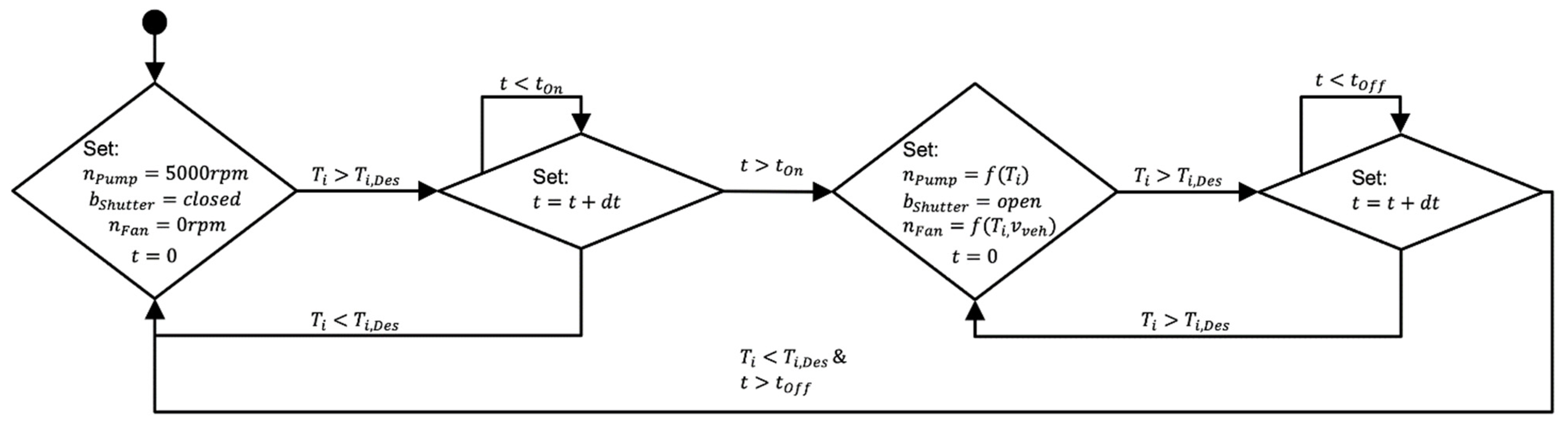
6.1. Introduction: Driving Cycles and Rule-Based Baseline Strategy

For this contribution, three different driving cycles were investigated, namely the WLTC, the so-called Eifel Cycle, and a Highway Cycle. The velocity profiles can be seen in Figure 7. The WLTC is well known for its length of 23.26 km while the Eifel Cycle is a cycle on rural roads with a highway section at the end. The latter passes the Eifel area in Western Germany, which has many uphill and downhill slopes. It has slopes of around ±4.7%, a length of 87.7 km and an altitude between 77 m up to 586 m. It is commonly used for real driving emission (RDE) homologation purposes as well. The highway cycle was a round trip from Aachen (Germany) to Cologne (Germany) and had a length of 125 km. The Eifel Cycle and the Highway Cycle were based on measurements taken during real test drives.
In this section, the functionality of the rule-based controller is described, which is the baseline for the energy comparison. In Figure 8, the controller structure is depicted schematically in a simplified way, referring to the temperature-defined hysteresis loops from [27], while the temperature limitations were chosen in accordance to prevent a boiling coolant and thermal failure [30]. Therefore, the default controls constitute the safety operation point for the PMSM and inverter, as described in [32,33].
For the rule-based strategy, the pump runs at a minimum of 5000 rpm in order to distribute the heat and cool the system. Moreover, the shutter is closed, which is why the fan is turned off. Each monitored temperature T i within the system is compared to its desired threshold T i , D e s . If a temperature exceeds its desired set point, a qualifying timer t counts for as long as the temperature is exceeded. When the timer surpasses the threshold t O n , the pump speed is increased depending on the temperature difference. In addition, the shutter is opened and the fan is activated. The fan speed depends on the maximum temperature exceedance, as well as the vehicle speed. With higher vehicle speeds, the relative air velocity increase by the fan is reduced. Thus, the fan speed is reduced with higher vehicle speeds. If all temperatures are below the desired threshold, a timer starts counting and when it exceeds the threshold t O f f , the system is set back to the default mode. The counting is reset if one of the temperatures exceeds its threshold during the qualification.

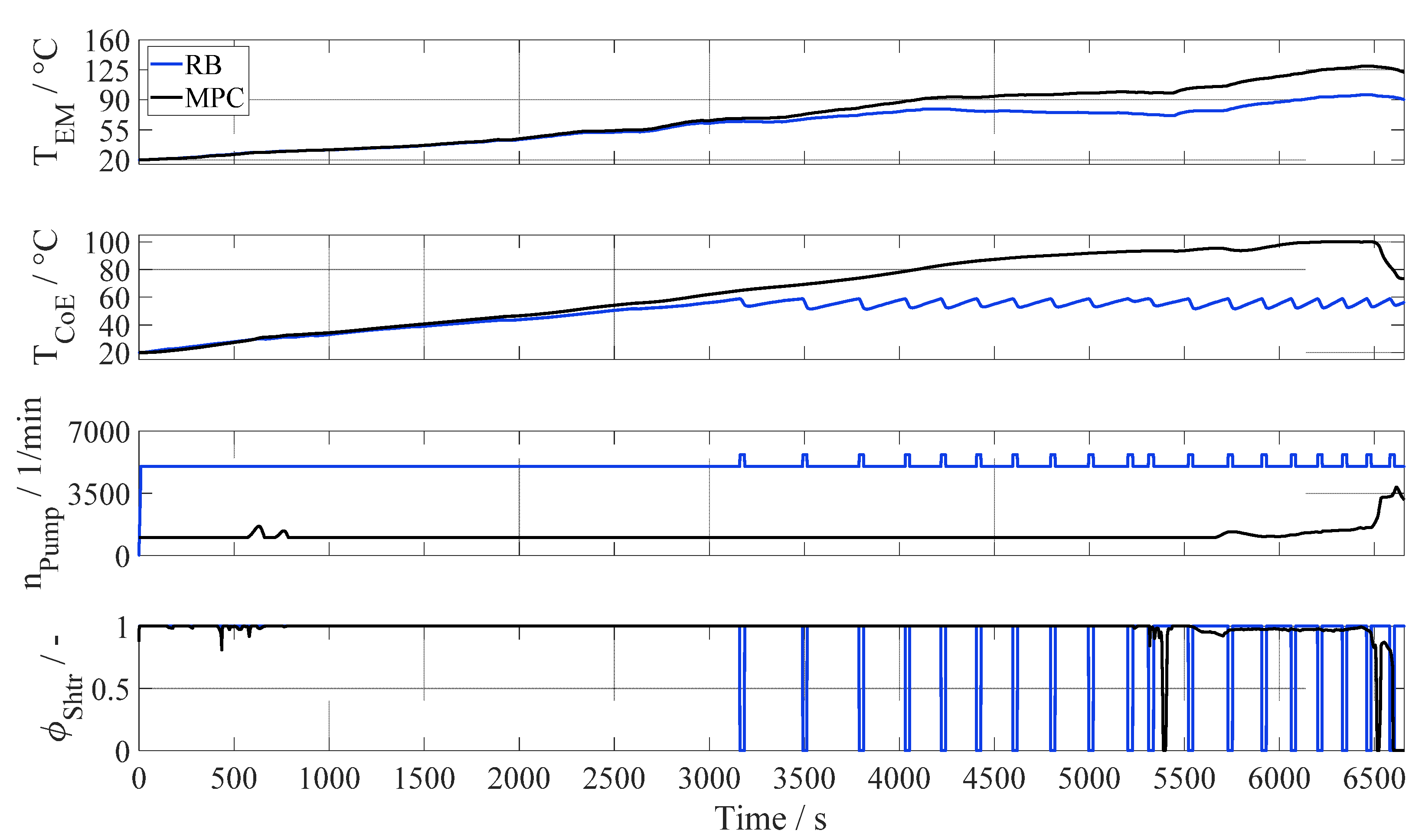
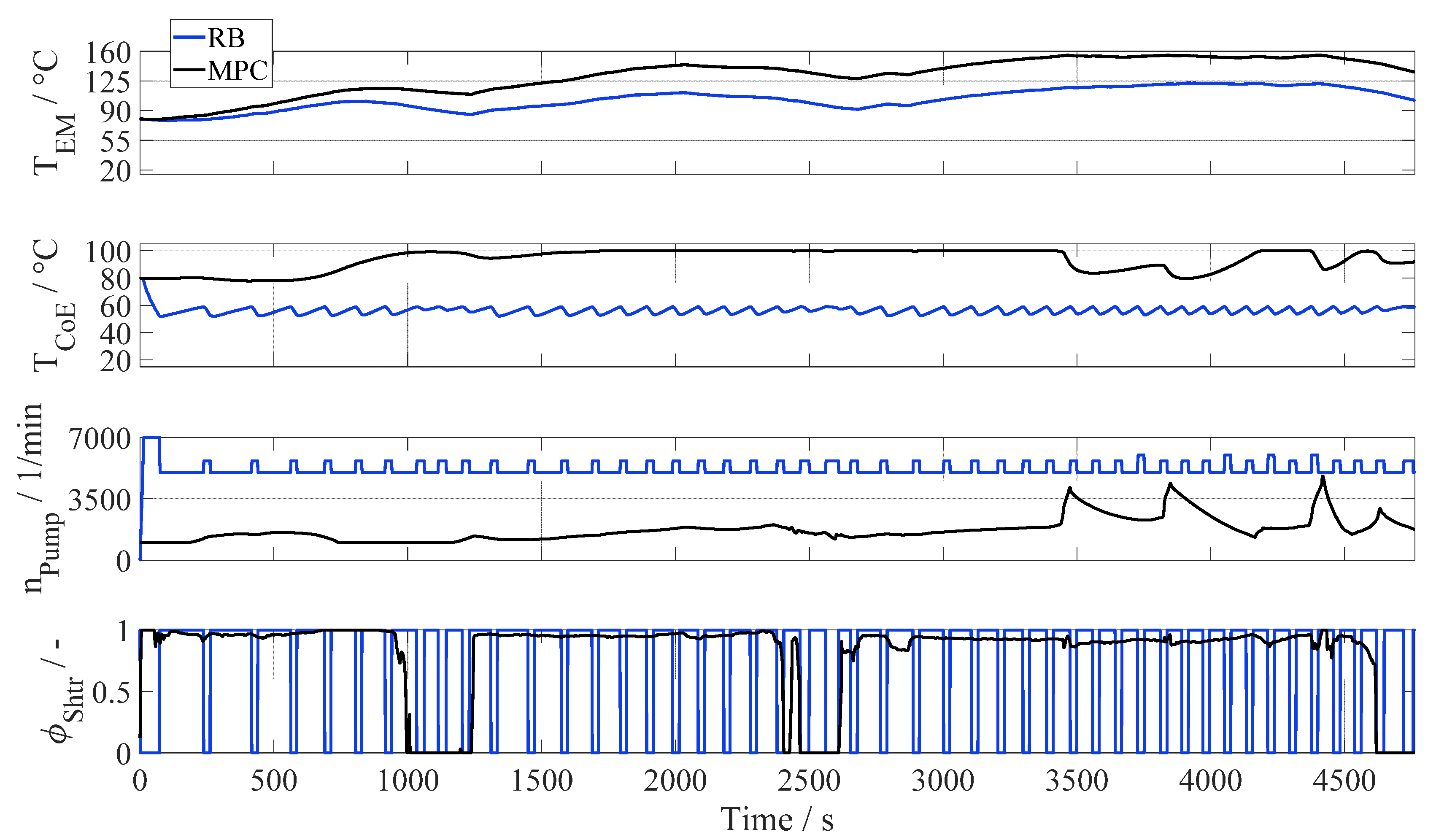
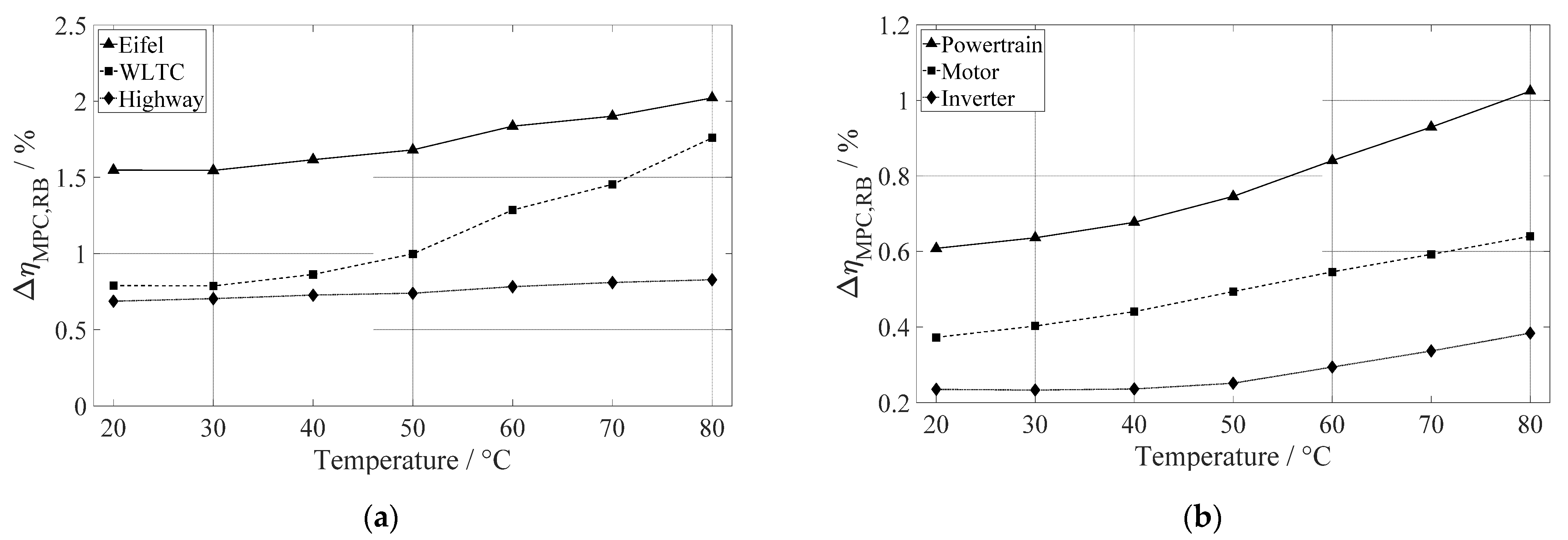
6.2. Evaluation of the Potential of the Economic Model Predictive Control

In this section, the energy comparison of the different controllers is presented. Two controllers were considered in detail—a rule-based controller (RB) with a shutter and the economic model predictive control (MPC) with a shutter. Afterwards, a comparison between the same MPC and the rule-based controller without a shutter is presented. All simulations were carried out considering an ambient temperature of 20 °C.
For analysing the system, an energy balance around the powertrain including the DCDC converter and the low voltage actuators is shown in (22). The energy balance boundaries are in line with the system of interest shown in Figure 1b.
E H V = E W h e e l + E E M , L o s s + E I n v , L o s s + E e l , P u m p + E e l , F a n η D C D C
The energy balance considers the high voltage energy draw E H V for the respective controller case. The gear box and final drive efficiencies were assumed to be ideal and were therefore excluded. The total wheel energy E W h e e l includes the energy demand reduction by the shutter. The latter shifts the torque delivered by the motor and inverter and by this, also influences the losses, as shown in Figure 3. For the acceleration case, the energy demands E E M , L o s s , E I n v , L o s s , E e l , P u m p , and E e l , F a n are positive, which means an increase of the energy drawn from the HV system, while during recuperation, all loss terms decrease the energy that is stored in the HV battery. Subtracting the recuperated energy from the energy demand during acceleration leads to the overall energy demand, which is finally used for the efficiency calculation.
The first cycle to be evaluated was the Eifel Cycle, with an ambient temperature of 20 °C, which was also the initial temperature of all the components. The results are depicted in Figure 9. In the following figures, the shutter position ϕ S h t r = 1 indicates a closed shutter, while ϕ S h t r = 0 reflects an open shutter. In the first half, the RB and the MPC both promote heating of the system to save energy by running the pumps at their minimum speed while keeping the shutter closed and the fan turned off. In rule-based strategies, it is common to maintain a high-volume flow to avoid derating by overheating. Thus, the pump runs at a base speed of 5000 rpm. The MPC has a minimum speed of 1000 rpm in order to avoid hot spots, as temperature exceedances can be omitted with this approach using the predictive information. For the economic MPC, the reason the system was not cooled is clear from the losses in Figure 3 and the speed trace in Figure 7. Due to the low to mid speeds and torques, the inverter losses were smaller at a high temperature, while the motor had generally small losses in this operation area. In addition, potential actuator costs supported the heating.
In the second half, starting at 3100 s, it can be seen that the pump and the shutter of the base strategy started to cool the system, as the coolant temperature after the motor T C o E was the first to exceed its target value. Since the cycle was very transient at this point, resulting in high losses, the base strategy repeatedly cooled the system until the temperature dropped sufficiently. Meanwhile, the MPC stayed in the heating mode, leading to a divergence of the motor, inverter, and coolant temperatures between the RB and MPC. The final temperature difference for the motor was 32.5 °C. The heating was targeted because over the deployed horizon of 600 s, the high motor temperature is beneficial due to the higher driving speeds ahead in the cycle. Around 5400 s, the shutter and the pump started to be controlled by the MPC to cool the system. This is because the end of the horizon 600 s later was predicted to exceed the coolant temperature limit. As it can be seen in Figure 9, the MPC controlled the coolant temperature along its limit by slightly opening the shutter and increasing the pump speed, consuming minimal actuation energy. The overall savings following (22) were 1.55% less energy consumption at the HV level. The elevated temperatures of the powertrain led to a 0.61% efficiency increase, while the rest was achieved by reduced actuator usage and the closed shutter.
Next to the Eifel Cycle, the Highway Cycle was analysed using a starting temperature of 80 °C. The starting temperature reflected that the starting point is after a battery charging break on the highway after a long drive. Thus, the prior loss-generated heat was already distributed. In Figure 10, the results for both controllers are depicted. As the coolant overheated at the beginning for the rule-based controller, it used the fan, shutter, and pump for maximum cooling. As before, the strategy then cooled whenever one of the temperatures exceeded its target temperature, leading to behaviour similar to what is shown in Figure 9. The maximum temperature over the cycle for the motor was 96 °C with the base controller.
On the other hand, the MPC opened the shutter slightly at the start of driving, since the predicted heat losses would have caused the coolant temperature to exceed due to the high load of the cycle. Around 1000 s until 1300 s, the velocity decreased significantly due to a traffic jam. Because of this, the MPC utilised the high-speed phase to save energy by closing the shutter at around 700 s and guiding the coolant close to its temperature limit.
At 1000 s, finally, the speed was low, so opening the shutter is associated with a low cost. This was required to avoid a temperature exceedance. Since the MPC already predicted the upcoming high velocity, it maintained the shutter open to invest in cooling at a low cost. However, as the cost due to increased losses at wheel level became high, the shutter almost fully closed when accelerating again. In the following, having the shutter slightly opened, the pump speed was increased in order to dissipate the heat such that the coolant again ran at its temperature limit. The procedure of the shutter opening at low speeds utilizing cooling at a low cost was repeated at around 2500 s and 2750 s. After this, the MPC kept the shutter slightly more open than before while increasing the pump speed. This was to maintain the motor temperature T E M below its temperature limit of 155 °C. The maximum temperature difference between the strategies for the motor was 59 °C, while the maximum inverter temperature difference was 30 °C. As the inverter has reduced efficiency in high-speed operations for elevated temperatures, the additional losses evened out with the benefit of the motor due to its higher temperature. However, the MPC had an HV power reduction of 0.83% compared to the rule-based strategy mainly by keeping the shutter closed and running the system at its temperature limits.
After analysing the traces in detail, Figure 11a shows a variation over all three cycles for a starting temperature range of 20–80 °C at a 20 °C ambient temperature. The WLTC shows increasing savings with rising temperatures, starting at 0.79–1.76%. At low starting temperatures, both control strategies promoted active heating. Thus, the majority of the savings for the MPC were based on a lower usage of the actuators. With an increasing start temperature, the rule-based strategy started to cool more, while the MPC remained in the heating phase due to the low transience of the cycle. While at a 20 °C starting temperature, the MPC saved only 0.02% due to the small motor temperature difference between the controller cases, a 0.37% savings was achieved at an 80 °C start temperature due to the increased motor temperature. This is a major contribution to increasing efficiency with a rising start temperature. The Highway Cycle had savings of 0.69–0.83% with an increasing start temperature. As seen in Figure 10, the inverter performed worse at high speeds under hot conditions, so the entire powertrain had additional losses of up to −0.04% with temperature variations. Nonetheless, the heating was functional as it enabled high shutter savings due to the high speeds, which were the main contributor to the savings in this case.
The third cycle to be evaluated was the Eifel Cycle, which had overall savings of 1.55–2.02%, as can be seen in Figure 11a. This includes all losses from (22). In contrast, in Figure 11b, only the efficiency increases due to temperature-dependent losses of the motor, the inverter, and the overall powertrain are depicted. Here, the start temperature variation was also considered. A clear trend can be seen that higher start temperatures were beneficial for the savings. The motor had temperature-dependent savings of 0.37–0.64%, while the inverter at high temperatures saved 0.24–0.38%, as a major share of the cycle is in the medium speed range where the inverter has NTC behaviour. Comparing the efficiency increase between 20 °C and 80 °C of 0.47% for all losses from Figure 11a with the gain of 0.41% for the powertrain in Figure 11b, it can be seen that the additional savings mainly increased due to the higher temperature levels of the MPC. As a result, the share of the powertrain regarding the overall savings at 20 °C starting temperature was 39% and increased to 51% at an 80 °C starting temperature.
As a final evaluation, the rule-based approach with no shutter (RB-NoShtr) was simulated again with a start temperature variation of 20–80 °C. The resulting efficiency differences to the MPC approach are depicted in Figure 12. In comparing Figure 12 with Figure 11a, it can be seen that the trends in savings for the different cycles were similar across the temperature variation, but the magnitude of the savings was higher. On the one hand, this was due to the reduced temperatures of the components because of the missing shutter. On the other hand, the MPC kept the shutter mostly closed in all cases, so that the drag coefficient was reduced. These effects increased the efficiency advantage for the Eifel Cycle to 3.7–4.2%. The absolute savings of the powertrain due to temperature-dependent efficiencies for this case were 1.2–1.67%, which in turn increased with the start temperature. The higher temperature-dependent savings compared to the rule-based case with a shutter were due to the colder components in the baseline approach, since the pump was running at least at 5000 rpm and the shutter was open, as before. The same applies to the WLTC, which had overall savings of 2.94–3.77%. For the Highway Cycle, savings of around 2.8% were achieved. As for the rule-based comparison with a shutter, the temperature-dependent gains of the motor balanced out with the losses of the inverter. Thus, the additional savings were due to the reduced drag coefficient, and therefore, the savings were mostly temperature independent.

7. Conclusions

In this paper, a novel approach was presented to utilise the temperature-dependent efficiencies of the powertrain for a BEV in combination with a grille shutter in front of the radiator to reduce the energy demand and promote active heating of the components.
After introducing the economic model predictive control approach, the system model was explained in detail, which used lumped parameter thermal networks. The model was parametrized and validated against transient wind tunnel measurements. Then, a comparison between the MPC and a rule-based controller with a shutter was made. For the analysis, the efficiency increase by the temperature-dependent loss mechanisms was given special attention. Furthermore, the comparison of the MPC to a rule-based strategy without a shutter was shown.
The main outcome is that temperature-dependent efficiencies are a relevant effect for inverters and permanent magnet synchronous machines in BEV applications. While it was shown that overall savings of up to 4.2% are possible, an efficiency increase at an HV level of up to 1.67% was achieved solely based on the temperature-dependent efficiencies of the powertrain. The savings resulted in a range increase for every battery charge—as a result, the battery can be sized smaller. This is one contributor to the goal of the CEVOLVER project, which is to enable long-distance travelling using small batteries [9]. As the components are being operated at their limits, the results imply an economic driver who closely follows a speed advice, which needs to be provided by another function, such as the eco-driving algorithm developed in the CEVOLVER project [80]. A sportive driver who does not follow the predicted speed profile can bring the system into derating or even cause damage amongst others due to the demagnetization of the permanent magnets. Considering a modified component design, for example, of the internal coolant routing, lower time constants, and thus, even higher efficiencies may be possible.
The savings, which were due in particular to the temperature difference, depended to a large extent on the drive cycle considered as well as on the ambient temperature. In future work, these effects shall be investigated more. Additionally, detailed models to simulate different temperatures within the components are necessary to better understand and exploit the thermal behaviour and will therefore be the subject of future work as well.

Author Contributions

Conceptualization, A.W., C.S., and J.A.; methodology, A.W., C.W., P.M., and B.K.; software, A.W., C.W., B.K., and B.C.; validation, A.W. and C.W.; formal analysis, A.W., P.M., and J.A.; investigation, A.W.; writing—original draft preparation, A.W.; writing—review and editing, C.S. and J.A.; visualization, A.W., C.W., B.K., P.M., and B.C.; supervision, C.S. and J.A.; project administration, J.A.; funding acquisition, C.S. and J.A. All authors have read and agreed to the published version of the manuscript.

Funding

This paper was created in the context of the CEVOLVER project and has received funding so labour cost were covered. This project has received funding from the European Union’s Horizon 2020 research and innovation programme under grant agreement No 824295. This publication reflects only the author's view. The Agency is not responsible for any use that may be made of the information it contains.
Energies 15 01476 i001

Institutional Review Board Statement

Not applicable.

Informed Consent Statement

Not applicable.

Data Availability Statement

All relevant data is presented within the article.

Conflicts of Interest

The authors declare no conflict of interest.

References

  1. International Energy Agency. Global EV Outlook 2020. Available online: https://www.iea.org/reports/global-ev-outlook-2020 (accessed on 27 January 2022).
  2. Deloitte. 2021 Global Automotive Consumer Study. Available online: https://www2.deloitte.com/content/dam/Deloitte/us/Documents/manufacturing/us-2021-global-automotive-consumer-study-global-focus-countries.pdf (accessed on 27 January 2022).
  3. Yang, Y.; Tan, Z.; Ren, Y. Research on Factors That Influence the Fast Charging Behavior of Private Battery Electric Vehicles. Sustainability 2020, 12, 3439. [Google Scholar] [CrossRef] [Green Version]
  4. Macioszek, E. Electric Vehicles—Problems and Issues. In Smart and Green Solutions for Transport Systems, Proceedings of the Scientific And Technical Conference Transport Systems Theory And Practice, Katowice, Poland, 16–18 September 2019; Advances in Intelligent Systems and Computing; Springer: Cham, Switzerland, 2019. [Google Scholar]
  5. Macioszek, E. E-mobility Infrastructure in the Górnośląsko—Zagłębiowska Metropolis, Poland, and Potential for Development. In Proceedings of the 5th World Congress on New Technologies, Lisbon, Portugal, 18–20 August 2019. [Google Scholar] [CrossRef]
  6. Ling, Z.; Cherry, C.R.; Wen, Y. Determining the Factors That Influence Electric Vehicle Adoption: A Stated Preference Survey Study in Beijing, China. Sustainability 2021, 13, 11719. [Google Scholar] [CrossRef]
  7. De Cauwer, C.; Verbeke, W.; Coosemans, T.; Faid, S.; van Mierlo, J. A Data-Driven Method for Energy Consumption Prediction and Energy-Efficient Routing of Electric Vehicles in Real-World Conditions. Energies 2017, 10, 608. [Google Scholar] [CrossRef] [Green Version]
  8. Tomaszewska, A.; Chu, Z.; Feng, X.; O’Kane, S.; Liu, X.; Chen, J.; Ji, C.; Endler, E.; Li, R.; Liu, L.; et al. Lithium-ion battery fast charging: A review. eTransportation 2019, 1, 100011. [Google Scholar] [CrossRef]
  9. Uniresearch, B.V. CEVOLVER—Connected Electric Vehicle Optimized for Life, Value, Efficiency and Range. Project Homepage. Available online: https://cevolver.eu/ (accessed on 29 January 2022).
  10. Brandes, H.; Faye, I.; Döges, V. Analysis of electric vehicle design and travel based on long trip capabilities. In Proceedings of the 8th Transport Research, Helsinki, Finland, 27–30 April 2020. [Google Scholar]
  11. Drgoňa, J.; Arroyo, J.; Cupeiro Figueroa, I.; Blum, D.; Arendt, K.; Kim, D.; Ollé, E.P.; Oravec, J.; Wetter, M.; Vrabie, D.L.; et al. All you need to know about model predictive control for buildings. Annu. Rev. Control 2020, 50, 190–232. [Google Scholar] [CrossRef]
  12. Dong, B.; Lam, K.P. A real-time model predictive control for building heating and cooling systems based on the occupancy behavior pattern detection and local weather forecasting. Build. Simul. 2014, 7, 89–106. [Google Scholar] [CrossRef]
  13. Oldewurtel, F.; Parisio, A.; Jones, C.N.; Gyalistras, D.; Gwerder, M.; Stauch, V.; Lehmann, B.; Morari, M. Use of model predictive control and weather forecasts for energy efficient building climate control. Energy Build. 2012, 45, 15–27. [Google Scholar] [CrossRef] [Green Version]
  14. Suda, T.; Namerikawa, T. Robust prediction and MPC-based optimal energy management for HVAC System. IFAC-PapersOnLine 2018, 51, 472–477. [Google Scholar] [CrossRef]
  15. Paffumi, E.; Otura, M.; Centurelli, M.; Casellas, R.; Brenner, A.; Jahn, S. Driving Range and Cabin Temperature Performances at Different Ambient Conditions in Support to the Design of a User-Centric Efficient Electric Vehicle: The QUIET Project. In Proceedings of the 14th Conference on Sustainable Development of Energy, Water and Environment Systems 2019, Dubrovnik, Croatia, 1–6 October 2019. [Google Scholar]
  16. Wang, M.; Craig, T.; Wolfe, E.; LaClair, T.J.; Gao, Z.; Levin, M.; Demitroff, D.; Shaikh, F. Integration and Validation of a Thermal Energy Storage System for Electric Vehicle Cabin Heating; SAE Technical Paper 2017-01-0183; SAE International: Warrendale, PA, USA, 2017. [Google Scholar] [CrossRef]
  17. Lohse-Busch, H.; Duoba, M.; Rask, E.; Stutenberg, K.; Gowri, V.; Slezak, L.; Anderson, D. Ambient Temperature (20°F, 72°F and 95°F) Impact on Fuel and Energy Consumption for Several Conventional Vehicles, Hybrid and Plug-In Hybrid Electric Vehicles and Battery Electric Vehicle; SAE Technical Paper 2013-01-1462; SAE International: Warrendale, PA, USA, 2013. [Google Scholar] [CrossRef]
  18. Chowdhury, S.; Leitzel, L.; Zima, M.; Santacesaria, M.; Titov, G.; Lustbader, J.; Rugh, J.; Winkler, J.; Khawaja, A.; Govindarajalu, M. Total Thermal Management of Battery Electric Vehicles (BEVs); SAE Technical Paper 2018-37-0026; SAE International: Warrendale, PA, USA, 2018. [Google Scholar] [CrossRef] [Green Version]
  19. De Nunzio, G.; Sciarretta, A.; Steiner, A.; Mladek, A. Thermal management optimization of a heat-pump-based HVAC system for cabin conditioning in electric vehicles. In Proceedings of the 2018 Thirteenth International Conference on Ecological Vehicles and Renewable Energies (EVER), Monte-Carlo, Monaco, 10–12 April 2018; pp. 1–7, ISBN 978-1-5386-5966-3. [Google Scholar]
  20. Dvorak, D.; Basciotti, D.; Gellai, I. Demand-Based Control Design for Efficient Heat Pump Operation of Electric Vehicles. Energies 2020, 13, 5440. [Google Scholar] [CrossRef]
  21. Amini, M.R.; Sun, J.; Kolmanovsky, I. Two-Layer Model Predictive Battery Thermal and Energy Management Optimization for Connected and Automated Electric Vehicles. 2018. Available online: http://arxiv.org/pdf/1809.10002v1 (accessed on 27 January 2022).
  22. Park, S.; Ahn, C. Computationally Efficient Stochastic Model Predictive Controller for Battery Thermal Management of Electric Vehicle. IEEE Trans. Veh. Technol. 2020, 69, 8407–8419. [Google Scholar] [CrossRef]
  23. Lopez Sanz, J.; Ocampo-Martinez, C.; Alvarez-Florez, J.; Moreno Eguilaz, M.; Ruiz-Mansilla, R.; Kalmus, J.; Graber, M.; Lux, G. Nonlinear Model Predictive Control for Thermal Management in Plug-in Hybrid Electric Vehicles. IEEE Trans. Veh. Technol. 2016, 66, 3632–3644. [Google Scholar] [CrossRef]
  24. Negandhi, V.; Jung, D.; Shutty, J. Active Thermal Management with a Dual Mode Coolant Pump. SAE Int. J. Passeng. Cars—Mech. Syst. 2013, 6, 817–825. [Google Scholar] [CrossRef]
  25. Karnik, A.Y.; Fuxman, A.; Bonkoski, P.; Jankovic, M.; Pekar, J. Vehicle Powertrain Thermal Management System Using Model Predictive Control. SAE Int. J. Mater. Manf. 2016, 9, 525–533. [Google Scholar] [CrossRef]
  26. Karnik, A.; Pachner, D.; Fuxman, A.M.; Germann, D.; Jankovic, M.; House, C. Model Predictive Control for Engine Powertrain Thermal Management Applications; SAE Technical Paper 2015-01-0336; SAE International: Warrendale, PA, USA, 2015. [Google Scholar] [CrossRef]
  27. Hemmati, S.; Doshi, N.; Hanover, D.; Morgan, C.; Shahbakhti, M. Integrated cabin heating and powertrain thermal energy management for a connected hybrid electric vehicle. Appl. Energy 2021, 283, 116353. [Google Scholar] [CrossRef]
  28. Wei, C.; Hofman, T.; Ilhan Caarls, E.; van Iperen, R. Integrated Energy and Thermal Management for Electrified Powertrains. Energies 2019, 12, 2058. [Google Scholar] [CrossRef] [Green Version]
  29. FEV GmbH. Smart Smart Wheels: Mobil im Internet der Energie. Available online: https://www.tib.eu/de/suchen/id/TIBKAT:796892903?cHash=1c0b077b1aac701cdff3227bbe895fad (accessed on 1 January 2022).
  30. Wulff, C.; Manns, P.; Pischinger, S. Optimum Cooling Circuit Control for Electric Drivetrains for Increased Driving Range. In Proceedings of the 28th Aachen Colloquium Automobile and Engine Technology, Aachen, Germany, 7–9 October 2019; pp. 1365–1377. [Google Scholar]
  31. Pierburg Pump Technology GmbH. CWA 100-2: Electrical Water Pump. Available online: https://www.tecomotive.com/de/produkte/CWA100.html (accessed on 27 January 2022).
  32. Holger Schmidt. Technical Data And Startup: DMC514, DMC524, DMC534, DMC544. Available online: https://manualzz.com/doc/7452231/2---brusa (accessed on 27 January 2022).
  33. BRUSA. HSM1—Hybrid Synchronous Motor: Optimum Performance from Zero Speed. Available online: https://www.brusa.biz/portfolio/hsm1-6-17-12/ (accessed on 27 January 2022).
  34. Albin Rajasingham, T. Nonlinear Model Predictive Control of Combustion Engines: From Fundamentals to Applications, 1st ed.; Springer International Publishing: Cham, Switzerland, 2021; ISBN 978-3-030-68009-1. [Google Scholar]
  35. Grüne, L.; Pannek, J. Nonlinear Model Predictive Control: Theory and Algorithms, 2nd ed.; Springer International Publishing: Cham, Switzerland, 2016; ISBN 978-3-319-46024-6. [Google Scholar]
  36. Ellis, M.; Liu, J.; Christofides, P.D. Economic Model Predictive Control: Theory, Formulations and Chemical Process Applications; Springer International Publishing: Cham, Switzerland, 2017; ISBN 978-3-319-41108-8. [Google Scholar]
  37. Rawlings, J.B.; Mayne, D.Q.; Diehl, M. Model Predictive Control: Theory, Computation, and Design, 2nd ed.; Nob Hill Publishing: Madison, WI, USA, 2017; ISBN 9780975937730. [Google Scholar]
  38. Verschueren, R.; Frison, G.; Kouzoupis, D.; Frey, J.; van Duijkeren, N.; Zanelli, A.; Novoselnik, B.; Albin, T.; Quirynen, R.; Diehl, M. Acados: A Modular Open-Source Framework for Fast Embedded Optimal Control. 2019. Available online: http://arxiv.org/pdf/1910.13753v3 (accessed on 27 January 2022).
  39. Frison, G.; Kouzoupis, D.; Sartor, T.; Zanelli, A.; Diehl, M. BLASFEO: Basic linear algebra subroutines for embedded optimization. ACM Trans. Math. Softw. 2018, 44, 1–30. [Google Scholar] [CrossRef] [Green Version]
  40. Frison, G.; Diehl, M. Hpipm: A High-Performance Quadratic Programming Framework for Model Predictive Control. 2020. Available online: http://arxiv.org/pdf/2003.02547v2 (accessed on 27 January 2022).
  41. Verschueren, R.; Zanon, M.; Quirynen, R.; Diehl, M. A Sparsity Preserving Convexification Procedure for Indefinite Quadratic Programs Arising in Direct Optimal Control. SIAM J. Optim. 2017, 27, 2085–2109. [Google Scholar] [CrossRef]
  42. Yang, Y.; Bilgin, B.; Kasprzak, M.; Nalakath, S.; Sadek, H.; Preindl, M.; Cotton, J.; Schofield, N.; Emadi, A. Thermal management of electric machines. IET Electr. Syst. Transp. 2017, 7, 104–116. [Google Scholar] [CrossRef] [Green Version]
  43. Bauer, D. Verlustanalyse bei Elektrischen Maschinen für Elektro- und Hybridfahrzeuge zur Weiterverarbeitung in Thermischen Netzwerkmodellen; Springer: Wiesbaden, Germany, 2019; ISBN 978-3-658-24271-8. [Google Scholar]
  44. Dutta, R.; Chong, L.; Rahman, F.M. Analysis and Experimental Verification of Losses in a Concentrated Wound Interior Permanent Magnet Machine. PIER B 2013, 48, 221–248. [Google Scholar] [CrossRef] [Green Version]
  45. Németh-Csóka, M. Thermisches Management elektrischer Maschinen; Springer: Wiesbaden, Germany, 2018; ISBN 978-3-658-20132-6. [Google Scholar]
  46. Binder, A. Elektrische Maschinen und Antriebe; Springer: Berlin/Heidelberg, Germany, 2012; ISBN 978-3-540-71849-9. [Google Scholar]
  47. Baranski, M.; Szelag, W.; Lyskawinski, W. Analysis of the Partial Demagnetization Process of Magnets in a Line Start Permanent Magnet Synchronous Motor. Energies 2020, 13, 5562. [Google Scholar] [CrossRef]
  48. Ehsani, M.; Wang, F.-Y.; Brosch, G.L. (Eds.) Transportation Technologies for Sustainability; Springer: New York, NY, USA, 2013; ISBN 978-1-4614-5843-2. [Google Scholar]
  49. Doppelbauer, M. Grundlagen der Elektromobilität; Springer: Wiesbaden, Germany, 2020; ISBN 978-3-658-29729-9. [Google Scholar]
  50. Das, S.C.; Narayanan, G.; Tiwari, A. Experimental study on the dependence of IGBT switching energy loss on DC link voltage. In Proceedings of the 2014 IEEE International Conference on Power Electronics, Drives and Energy Systems (PEDES), Mumbai, India, 16–19 December 2014. [Google Scholar] [CrossRef]
  51. Yang, J.; Che, Y.; Ran, L.; Jiang, H. Evaluation of Frequency and Temperature Dependence of Power Losses Difference in Parallel IGBTs. IEEE Access 2020, 8, 104074–104084. [Google Scholar] [CrossRef]
  52. Kolar, J.; Drofenik, U. A General Scheme for Calculating Switching- and Conduction-Losses of Power Semiconductors in Numerical Circuit Simulations of Power Electronic Systems. In Proceedings of the International Power Electronics Conference, Niigata, Japan, 4–8 April 2005. [Google Scholar]
  53. Wallscheid, O. Thermal Monitoring of Electric Motors: State-of-the-Art Review and Future Challenges. IEEE Open J. Ind. Applicat. 2021, 2, 204–223. [Google Scholar] [CrossRef]
  54. Chen, B.; Wulff, C.; Etzold, K.; Manns, P.; Birmes, G.; Andert, J.; Pischinger, S. A Comprehensive Thermal Model For System-Level Electric Drivetrain Simulation With Respect To Heat Exchange Between Components. In Proceedings of the 2020 19th IEEE Intersociety Conference on Thermal and Thermomechanical Phenomena in Electronic Systems (ITherm), Orlando, FL, USA, 21–23 July 2020; pp. 558–567, ISBN 978-1-7281-9764-7. [Google Scholar]
  55. Demetriades, G.D.; De La Parra, H.Z.; Andersson, E.; Olsson, H. A Real-Time Thermal Model of a Permanent-Magnet Synchronous Motor. IEEE Trans. Power Electron. 2010, 25, 463–474. [Google Scholar] [CrossRef]
  56. Huber, T.; Bocker, J.; Peters, W. A Low-order Thermal Model for Monitoring Critical Temperatures in Permanent Magnet Synchronous Motors. In Proceedings of the 7th IET International Conference on Power Electronics, Machines and Drives (PEMD 2014), Manchester, UK, 8–10 April 2014; pp. 1–6, ISBN 978-1-84919-815-8. [Google Scholar]
  57. Boglietti, A.; Cavagnino, A.; Staton, D.; Shanel, M.; Mueller, M.; Mejuto, C. Evolution and Modern Approaches for Thermal Analysis of Electrical Machines. IEEE Trans. Ind. Electron. 2009, 56, 871–882. [Google Scholar] [CrossRef] [Green Version]
  58. Scheuermann, U. AN1501: Estimation of Liquid Cooled Heat Sink Performance at Different Operation Conditions. Available online: https://www.semikron.com/dl/service-support/downloads/download/semikron-application-note-estimation-of-liquid-cooled-heat-sink-performance-at-different-operation-conditions-en-2015-10-16-rev-00/ (accessed on 27 January 2022).
  59. Wu, R.; Wang, H.; Pedersen, K.B.; Ma, K.; Ghimire, P.; Iannuzzo, F.; Blaabjerg, F. A Temperature-Dependent Thermal Model of IGBT Modules Suitable for Circuit-Level Simulations. IEEE Trans. Ind. Applicat. 2016, 52, 3306–3314. [Google Scholar] [CrossRef] [Green Version]
  60. MathWorks. Curve Fitting Toolbox: User’s Guide; MathWorks: Natick, MA, USA.
  61. Bergman, T.L.; Incropera, F.P.; De Witt, T.P.; Lavine, A.S. Fundamentals of Heat and Mass Transfer, 6th ed.; John Wiley & Sons: Hoboken, NJ, USA, 2007; ISBN 978-0471457282. [Google Scholar]
  62. Shah, R.K.; Sekulić, D.P. Fundamentals of Heat Exchanger Design; John Wiley & Sons: New York, NY, USA/Chichester, UK, 2003; ISBN 0-471-32171-0. [Google Scholar]
  63. Großmann, H. Pkw-Klimatisierung. Springer: Berlin/Heidelberg, Germany, 2013; ISBN 978-3-642-39840-7. [Google Scholar]
  64. Rajamani, R. Vehicle Dynamics and Control; Springer: Boston, MA, USA, 2012; ISBN 978-1-4614-1432-2. [Google Scholar]
  65. Pfeifer, C. Evolution of Active Grille Shutters; SAE Technical Paper 2014-01-0633; SAE International: Warrendale, PA, USA, 2014. [Google Scholar] [CrossRef]
  66. Bouilly, J.; Lafossas, F.; Mohammadi, A.; van Wissen, R. Evaluation of Fuel Economy Potential of an Active Grille Shutter by the Means of Model Based Development Including Vehicle Heat Management. SAE Int. J. Engines 2015, 8, 2394–2401. [Google Scholar] [CrossRef]
  67. Cho, Y.-C.; Chang, C.-W.; Shestopalov, A.; Tate, E. Optimization of Active Grille Shutters Operation for Improved Fuel Economy. SAE Int. J. Passeng. Cars—Mech. Syst. 2017, 10, 563–572. [Google Scholar] [CrossRef]
  68. El-Sharkawy, A.E.; Kamrad, J.C.; Lounsberry, T.H.; Baker, G.L.; Rahman, S.S. Evaluation of Impact of Active Grille Shutter on Vehicle Thermal Management. SAE Int. J. Mater. Manf. 2011, 4, 1244–1254. [Google Scholar] [CrossRef]
  69. Wolf, T. Developing a Theory for Active Grille Shutter Aerodynamics—Part 1: Base Theory; SAE Technical Paper 2019-01-5063; SAE International: Warrendale, PA, USA, 2019. [Google Scholar] [CrossRef]
  70. Kremheller, A. The Aerodynamics Development of the New Nissan Qashqai; SAE Technical Paper 2014-01-0572; SAE International: Warrendale, PA, USA, 2014. [Google Scholar] [CrossRef]
  71. Blacha, T.; Islam, M. The Aerodynamic Development of the New Audi Q5. SAE Int. J. Passeng. Cars—Mech. Syst. 2017, 10, 638–648. [Google Scholar] [CrossRef]
  72. Larose, G.; Belluz, L.; Whittal, I.; Belzile, M.; Klomp, R.; Schmitt, A. Evaluation of the Aerodynamics of Drag Reduction Technologies for Light-duty Vehicles: A Comprehensive Wind Tunnel Study. SAE Int. J. Passeng. Cars—Mech. Syst. 2016, 9, 772–784. [Google Scholar] [CrossRef]
  73. Larson, L.; Woodiga, S.; Gin, R.; Lietz, R. Aerodynamic Investigation of Cooling Drag of a Production Sedan Part 1: Test Results. SAE Int. J. Passeng. Cars—Mech. Syst. 2017, 10, 628–637. [Google Scholar] [CrossRef]
  74. Klingbeil, M.; Weissert, J.; Yilmaz, Z. The new Porsche 911 Carrera—Evolution in aerodynamics, thermal management and heat protection. In 16. Internationales Stuttgarter Symposium; Bargende, M., Reuss, H.-C., Wiedemann, J., Eds.; Springer: Wiesbaden, Germany, 2016; pp. 315–330. ISBN 978-3-658-13254-5. [Google Scholar]
  75. Feng, L.; Wikander, J.; Li, Z. Fuel Minimization of the Electric Engine Cooling System With Active Grille Shutter by Iterative Quadratic Programming. IEEE Trans. Veh. Technol. 2020, 69, 2621–2635. [Google Scholar] [CrossRef]
  76. Li, J.; Deng, Y.; Wang, Y.; Su, C.; Liu, X. CFD-Based research on control strategy of the opening of Active Grille Shutter on automobile. Case Stud. Therm. Eng. 2018, 12, 390–395. [Google Scholar] [CrossRef]
  77. Shigarkanthi, V.; Damodaran, V.; Soundararaju, D.; Kanniah, K. Application of Design of Experiments and Physics Based Approach in the Development of Aero Shutter Control Algorithm; SAE Technical Paper 2011-01-0155; SAE International: Warrendale, PA, USA, 2011. [Google Scholar] [CrossRef]
  78. Scherer, A. Neuronale Netze; Vieweg+Teubner Verlag: Wiesbaden, Germany, 1997; ISBN 978-3-528-05465-6. [Google Scholar]
  79. Wolf, T. Developing a Theory for Active Grille Shutter Aerodynamics—Part 2: Effect of Flap Thickness and Shape; SAE Technical Paper 2019-01-5095; SAE International: Warrendale, PA, USA, 2019. [Google Scholar] [CrossRef]
  80. Ngo, C.; Solano-Araque, E.; Aguado-Rojas, M.; Sciarretta, A.; Chen, B.; Baghdadi, M.E. Real-time eco-driving for connected electric vehicles. IFAC-PapersOnLine 2021, 54, 126–131. [Google Scholar] [CrossRef]
Figure 1. Overview of the system setup: (a) thermal system layout and control inputs; (b) electrical and mechanical layout of the powertrain.
Energies 15 01476 g001
Figure 2. Measurement setup of motor and inverter for the temperature-dependent efficiency evaluation with active component conditioning [30].
Energies 15 01476 g002
Figure 3. Temperature-dependent losses: (a) loss differences for the PMSM when increasing the temperature from 30 °C to 110 °C at 400 V supply voltage; (b) loss differences for the inverter when increasing the temperature from 30 °C to 110 °C at 400 V supply voltage.
Energies 15 01476 g003
Figure 4. Lumped parameter thermal networks for: (a) electric motor; (b) inverter.
Energies 15 01476 g004
Figure 5. Shutter modelling regarding: (a) relative drag coefficient increase as in Equation (21); (b) relative air mass flow to radiator.
Energies 15 01476 g005
Figure 6. System validation of the transient temperature for the powertrain plant model based on the US06 driving cycle at an ambient temperature around 20 °C.
Energies 15 01476 g006
Figure 7. Driving cycles considered in this contribution: WLTC, Eifel Cycle (with rural and highway parts), and Highway Cycle from Aachen to Cologne.
Energies 15 01476 g007
Figure 8. Simplified logic of rule-based controller for pump and fan speed as well as for shutter position depending on vehicle velocity and component temperatures.
Energies 15 01476 g008
Figure 9. Comparison of MPC and rule-based strategy (RB) regarding motor temperature T E M , motor outlet coolant temperature T C o E , pump speed n P u m p , and shutter position ϕ S h t r for the Eifel Cycle at 20 °C initial component temperature and 20 °C ambient temperature.
Energies 15 01476 g009
Figure 10. Comparison of MPC and rule-based strategy (RB) regarding motor temperature T E M , motor outlet coolant temperature T C o E , pump speed n P u m p , and shutter position ϕ S h t r for the Highway Cycle at 80 °C initial component temperature and 20 °C ambient temperature.
Energies 15 01476 g010
Figure 11. Efficiency increase using MPC in comparison to a rule-based strategy with shutter (RB) for component starting temperatures of 20–80 °C at 20 °C ambient temperature: (a) overall efficiency increase for all three driving cycles; (b) temperature-based efficiency increase for motor, inverter, and overall powertrain for the Eifel Cycle.
Energies 15 01476 g011
Figure 12. Overall efficiency increase for all three driving cycles using MPC in comparison to a rule-based strategy without shutter (RB-NoShtr) for component starting temperatures of 20–80 °C at 20 °C ambient temperature.
Energies 15 01476 g012
Table 1. Vehicle parameters for longitudinal model.
Vehicle ParameterValue
Vehicle typeBEV
Gross   weight :   m [kg]1335
Gear   ratio :   i G e a r [-]9.59
Drag   coefficient :   c d [-]0.325
Front area: A [m2]2.1
Dyn .   tyre   radius :   r d y n [m]0.27
Rolling   resistance   coefficient   f r   [-]0.0107
Publisher’s Note: MDPI stays neutral with regard to jurisdictional claims in published maps and institutional affiliations.

