Design of a Microscale Refrigeration System for Optimizing the Usable Space in Compact Refrigerators

Abstract

This research aims to enter the miniature refrigeration machine sector with the objective of designing a small scale unit while maintaining a competitive coefficient of performance (COP), comparing with a Peltier plates system. To this end, a research of the current technology was carried out in order to obtain indicative values on the scales that were being worked on and their application. After the previous research, a refrigeration cycle was designed in EES (engineering equation solver). From this design, different conclusions were obtained: (1) The correct sizing of the compressor revolutions together with its displacement is crucial for the equipment to be able to provide the desired cooling capacity. (2) In order to obtain the desired cooling capacity in the microscale refrigeration system, the heat exchangers must have fins. (3) Of the analysed refrigerants, R600a is the best choice, as it shows favourable characteristics (high COP and low compression ratio) when working in this type of cycle.

1. Introduction

This project responds to present and future energy saving needs in a European and international context. Within this framework of growing and urgent requirements to meet energy saving objectives in order to mitigate the actions that cause progressive climate change, it is necessary to be able to carry out sustainable developments in the face of the scarcity of current energy resources. Thus, this proposal focuses on energy saving that has an impact on the reduction in domestic electricity consumption with both local and international consequences. This project focuses on research into new ultra compact, energy efficient refrigeration solutions using vapour compression refrigeration cycle technology, to meet the challenges of a new generation of cooling and air-conditioning systems. Currently, most of these chillers use thermoelectric modules or Peltier plates for cooling, as this technology allows the cooling to be carried out in a very small volume and with very little noise.

In order to find a more efficient solution to the demand of this sector, the present project aims to develop a cooling solution to replace Peltier plates, maintaining the characteristic of compactness but increasing energy efficiency. To this end, the project aims to design and develop a new device based on the fluid compression refrigeration cycle, with dimensions similar to those of a thermoelectric module (40 × 40 × 20 mm), but with a performance between 2 and 4, considerably higher than the 0.2 ÷ 1 offered by thermoelectricity.

2. State of the Art

Vapour compression refrigeration (VCR) is the most widely used system for refrigeration and cooling in various fields, such as buildings, vehicles, food preservation, etc. This is due to its large capacity and high efficiency in converting electrical or mechanical energy into energy for cooling. In the building sector, HVAC-R systems (heating, ventilation, air conditioning and refrigeration) are the ones that consume the most energy, representing approximately 40–50% of total building energy consumption [1]. In the case of cooling electronic devices, the consumption almost doubles every two years, recently accounting for 1.12–1.5% of the total electricity consumption worldwide. To dissipate all the heat generated by these electronic devices, cooling systems have to operate continuously, with the resulting rise energy consumption [2].

Heat pump (HP) systems are mechanical systems driven by electrical energy with the objective of transferring heat from one heat source to another heat source for dissipation. The vast majority of HPs work on the vapour compression cycle (VCC) principle (Figure 1), which consists of an external heat exchanger (HX) (as evaporator), a compressor, an internal HX (as condenser) and an expansion valve. To transport the heat in the closed HP cycle, a volatile fluid, known as refrigerant fluid [3], is used.

In the condenser and evaporator HXs, heat is transferred between the refrigerant fluid and the heat source and dissipating medium fluids, known as secondary fluids. Depending on the HP, the dissipating medium can be water or air. In addition, the heat sources depend on the HP, the most common being ambient air, groundwater reservoirs or surface water reservoirs. The combination of these heat sources and heat sinks defines the HP classification.

Miniature vapour compression refrigeration (MVCR) is an alternative solution to the energy use problems mentioned above, which has great advantages in energy consumption, cooling capacity, efficiency and compactness. Therefore, MVCR is considered one of the most promising technologies for cooling where space is limited [4].

The miniaturization of components is a major issue in the proposed study. There are several possibilities for compact compressors, including reciprocating, centrifugal, rotary vane, or linear. Miniaturization is not the only requirement of MVCR; one of the most important points is how to achieve excellent cooling performance based on the miniaturization of the system. It is well known that larger systems are generally more thermodynamically efficient than smaller systems, which can be verified by the correlation of Alalaimi et al. [5]; therefore, one of the main objectives of the project is to develop a numerical model to characterize the behaviour of an MVCR. Then, the most relevant parameters are identified and analysed in order to define the MVCR, which complies with the specified characteristics:

• Cooling capacity around 100 W (to improve the energy behaviour of a refrigeration system based on Peltiers, it should be at least 70 W).
• Small size of the system, with a section around 40 × 40 mm.
• Better energy performance than a Peltier plate (COP higher than 1).

2.1. Integral Solution

To begin with, it is necessary to know the state of the art of the technology to be implemented. To this end, a search has been carried out for those cases where an MVCR system has been studied, built and put into operation. Although most of the cases are aimed at cooling electronic components, these studies will serve as a reference when carrying out the design objective of this project.

Different numerical studies have been found in the literature, such as the one developed by Heppner et al. [6]. It makes use of a Wankel compressor that provides six compression strokes per revolution instead of a single compression stroke, like other piston type compressors. This design achieves a theoretical compression ratio of 4.7:1. The system is designed to remove 45 W of heat at 1000 rpm using an R-134a refrigerant with a theoretical performance coefficient of 4.6. The next system in order of cooling capacity would be the one developed by Chiriac et al. [7], who numerically designed a miniature R-134a refrigeration system for cooling electronic components. The system was estimated to achieve a cooling capacity of between 20 W and 100 W with a COP of up to 4.5. Finally, Mancin et al. [8], who used a linear compressor operating at constant speed, obtained the highest cooling capacity in the design. The cooling capacity ranged from 37 W to 374 W, while the COP ranged from 1.05 to 5.80.

In terms of experimental prototypes, Mongia et al. [9] designed and manufactured a miniature R-600a system packaged in a laptop computer. The system achieved a cooling capacity of 40 W and a COP of approximately 2.25. Sung et al. [10] recently developed a very compact MVCR system with dimensions of 60 mm × 60 mm × 100 mm, whose the cooling capacity was 80 W with a COP of 2.15. Trutassanawin et al. [11] built a miniature R-134a system using a variable speed DC rotary compressor. The system, with dimensions of about 350 mm × 250 mm × 170 mm, produced a cooling power of 75–140 W and a COP of 1.13–1.35. Maveety et al. [12] developed a miniature R-134a system to cool a 2 U rack. The prototype was able to provide a cooling capacity of 130 W and the COP varied between 2.2 and 5.8. Chang et al. [13] constructed an R-134a system with dimensions of 350 mm × 160 mm × 120 mm. The system achieved a maximum cooling capacity of 150 W with a COP of 4.25. Poachaiyapoom et al. [14] made a prototype which was subjected to different conditions, including compressor speeds of between 3000 and 6000 rpm and heating powers of 100 W, 150 W and 200 W. The highest COP obtained was 9.25, at a compressor speed of 3000 rpm and a heating power of 200 W. Finally, the prototype designed by Wu and Du [15] was an RCVM system using a centrifugal compressor for chip heat dissipation, whose dimensions were 300 mm × 230 mm × 70 mm. The COP of the system was as high as 5.7–8.6.

2.2. Components: Compressor, Heat Exchangers and Expansion Valve

The compressor, in terms of miniaturization, is the most complicated component of the refrigeration system. Studies that have been carried out on electronic refrigeration applications, without considering the miniaturization of the elements, used small, commercially available (but not meso-scale) compressors. Some commercial compressors are designed to operate at large compression ratios (e.g., refrigerators), with poor performance at the relatively small compression ratios often desired for cooling electronic components.

Table 1. Summary of the main characteristics of the studies mentioned above.

Authors	Refrigerant	Power Supply	Dimensions (mm)	Cooling Capacity (W)	COP
Trutassanawin et al. [11]	R-134a	CC	350 × 250 × 170	75–140	1.13–1.35
Mongia et al. [9]	R-600	12 V		40	2.25
Chiriac et al. [7]	R-134a		numerical	20	4.5
Maveety et al. [12]	R-134a	24 V CC		130	2.5–5.8
Chang et al. [13]	R-134a		350 × 160 × 120	150	4.25
Yu-Ting Wu et al. [15]			300 × 230 × 70	experimental	5.7–8.6
Mancin et al. [8]				37–374	1.05–5.80
Sung et al. [10]			60 × 60 × 100	80	2.15
Poachaiyapoom et al. [14]				200	9.06
Heppner et al. [6]	R-134a		25 × 30x-	45	4.6

shows a summary of the characteristics of the systems introduced so far. In addition to this information,

Table 2. Summary of some of the main characteristics of the studies mentioned above.

Authors	Refrigerant	Compression Mechanism	Cooling Capacity (W)	Tevap/Tcond	Displacement (cm3/rev)
Carter et al. [16]	Air	Centrifugal	32	12/60	-
Shannon et at. [17]	R-134a	Diaphragm	3	20/50	-
Hao et al. [18]	Air	Alternative	350	12/60	-
Bash et al. [19]	R-134a	Acoustic	400	18/52	-
Maveety et al. [12]	R-134a	Gyratory	50–120	50/20	1.8
Unger et al. [20]	R-134a	Lineal	1500	20/60	-
Mongia et al. [9]	R-600a	-	50	55/90	-
Sathe et al. [21]	R-134a	Gyratory	500	15.7/39.4	1.4
Ernst et al. [22]	R-134a	Alternative	120–280	22/44	4.92
Sathe et al. [23]	R-134a	Diaphragm	80	-	-
Wu et al. [24]	Air	Centrifugal	32	12/60	-
Bradshaw et al. [25]	R-134a	Diaphragm	3	20/50	-
External Dimensions	Impulsion System	Velocity (rpm)	Lubricant Type	Mass (g)	Power (W)
-	Variable capacitance	400,000	-	-	9.57
-	Electrostatic	-	-	-	0.5
1 cm (diameter) × 0.1 cm high	Electrostatic	-	No oil	-	-
-	Linear variable reluctance motor	46,800	No oil	-	123
8.9 cm (diameter) × 6.4 cm high	DC brushless motor	3000–3900	Polyol ester	1300	6–22
7.5 cm (diameter)	Lineal motor	-	Gas system	-	500
-	CC motor	-	-	-	22.2
5.58 cm (diameter) × 7.74 cm high	DC brushless motor	6000	Polyol ester	562	66
5.08 × 10.2 × 7.6 cm	Two-stroke engine	10,500	Polyol ester	440	46
32 cm3	Electrostatic	6000	-	-	-
-	Variable capacitance	400,000	-	-	9.57
-	Electrostatic	-	-	-	0.5

presents more details on compressors that have been modelled, designed, built and/or tested in refrigeration applications for electronics and personal refrigeration. These projects present vapour compression refrigeration cycles with an emphasis on compressor design and the description of its characteristics.

In order to ensure the correct operation of the cycle, it is important to size the HXs according to the cycle parameters. In the present case, these HX would be the evaporator and the condenser. In general terms, the most commonly used HXs are those known as plate HXs, consisting of a pack of metal plates with holes for the two fluids; or tube HXs, consisting of cylindrical tubes inside a casing, where one fluid circulates inside the tubes and the other outside. However, these systems can take up more space than they are intended to occupy, so in the articles consulted, a majority of the evaporators and condensers proposed are microchannel evaporators and condensers.

The design of the condenser and evaporator is also of vital importance, as they will take up some of the considered space. The closest study on which the current project could be based is the one by Heppner et al. [6]. The condenser is designed as a tubular structure in the form of a serpentine with fins. Similarly, the evaporator has a very similar design to the condenser, the only exception being that the material between the coils is not removed. This additional material increases the thermal capacity of the evaporator and allows heat to be absorbed into the fluid from both sides and the object to be cooled. Figure 2 shows both HXs.

In a similar way, the heat exchangers designed by Ricardo et al. [26] use the plate HXs typology with different routes, (a) serpentine (b) nested (c) parallel with fins. Apart from the results obtained for the different types, the three alternatives manage to generate a cooling capacity of 110 W, which is similar to the power to be obtained in this project. The work carried out by Taijong Sung et al. [10] also uses microchannel as the structure for the condenser and evaporator, the latter having fins. The cooling capacity of this system is 80 W.

The expansion valve is the element in charge of lowering the refrigerant pressure from the condenser stage to the evaporator stage. During this process, the refrigerant enters the valve in liquid form and, during the expansion, the process part of the fluid evaporates, leaving the valve as a partial liquid–vapour mixture.

There are different types of expansion systems; however, in order to carry out the project, the bibliography was consulted to find out which systems are frequently used. Two main types of systems have been found: capillary tubes and solenoid valves.

The capillary tube is usually made of copper. It has a very small diameter in order to produce a pressure drop. The main advantage of the capillary tube is that it is a very simple system, while also meeting the requirement of compactness. At the same time, it is worth mentioning that it does not allow the flow rate to be adjusted, which could be a disadvantage when adjusting the thermodynamic cycle for other workloads.

Table 3. Summary of the dimensions of the capillary tubes consulted.

Authors	Length (m)	Diameter (mm)
Poachaiyapoom Akasit et al. [14]	0.96	1.58
R.K. Mongia et al. [9]	1.1	0.4
Taiwo Babarinde et al. [27]	1.5	-
Zhihui Wu et al. [28]	1.6–1.8–2	0.8
Yu-Ting Wu et al. [24]	0.8–0.9–1–1.1	0.64

shows the capillary tube dimensions of the articles consulted.

3. Design

The review of the literature on compact refrigeration systems has made it possible to draw a trajectory line for the development of a simulation model. Many of the articles reviewed use different simulation programmes to determine the feasibility of the system to be implemented. Although the purpose of the present project is to create the physical model, it is worth mentioning that it is of great interest to obtain a prototype that allows us to know the key parameters for the correct operation of the refrigeration system.

The equation-solving program EES [29] was used to create the model. This program allows the equations that characterise the refrigeration cycle to be introduced in order to obtain a series of results that will serve as design guidelines. The equations that relate to the parameters of the cycle, those that will be taken as inputs to the model, are decided before implementation in order to be able to vary their values and thus obtain the optimum values for the system.

3.1. Election of the Refrigerant

International legislation has imposed a number of restrictions on the use of hydrofluorocarbon refrigerants (HFCs) due to their environmental impact.

When deciding on the thermodynamic parameters to be evaluated during the analysis, two circumstances have been taken into account:

-

Firstly, the particular characteristics of an ultra compact model in terms of working pressures and temperatures. For this reason, the parameters to be analysed were the evaporator pressure, the condenser pressure, the compression ratio and the compressor outlet temperature.

-

Secondly, in order to develop a commercial product, it is necessary to evaluate the efficiency of the cycle, which is analysed through the COP of the cycle.

Specifically, the working conditions analysed are those detailed in

Table 4. Working conditions analysed.

Case	Tevaporation [°C]	Tcondensation [°C]
1	−5	25
2	0	25
3	0	30
4	5	30
5	8	30
6	10	30

:

In addition, as there is not much information available on equipment efficiencies in ultra compact applications, the behaviour of the different refrigerants has been analysed for four different isentropic compressor efficiencies, as can be seen in

Table 5. Isentropic efficiencies.

Case	ηs [-]
1	1.0
2	0.9
3	0.8
4	0.7

.

In total, the combination of all variants (7 refrigerants × 6 conditions × 4 efficiencies) would result in a total of 168 cycles. Finally, the total number of cases was 160, as the software used (EES—engineering equation solver) does not allow the properties of R513A to be evaluated for evaporation temperatures of 8 °C and 10 °C.

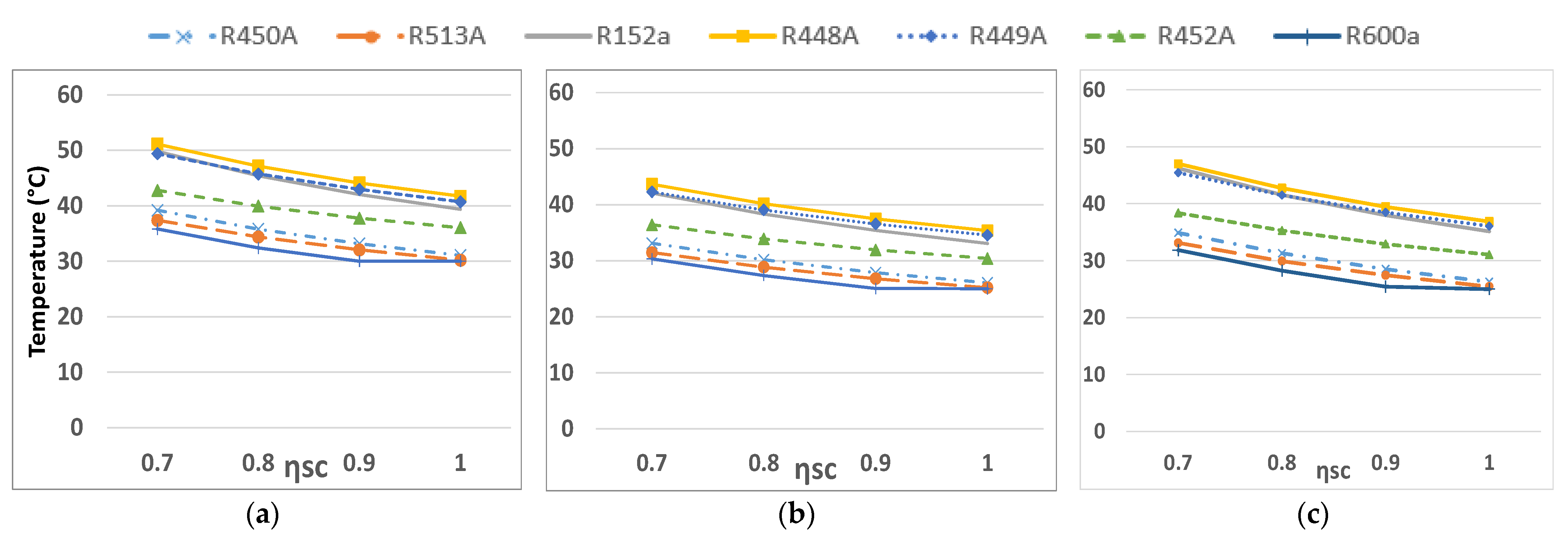
Figure 3 shows the COP values as a function of the isentropic efficiency of the compressor and the working fluid for the cases −5 °C/25 °C; 0 °C/25 °C and 0 °C/30 °C as an example. As can be seen in the different graphs (Figure 3), the behaviour is completely homogeneous for different temperatures, and this behaviour is repeated for all the cases analysed.

According to the graphs, it can be observed that:

-

The highest COP values are obtained with R152a and R600a, with minimal differences between them.

-

R513a and R450a have values similar to each other and somewhat lower than the two previous refrigerants.

-

Finally, the group formed by R448A, R449A and R452A have significantly lower values, between 0.9 and 1.6 COP points depending on the conditions.

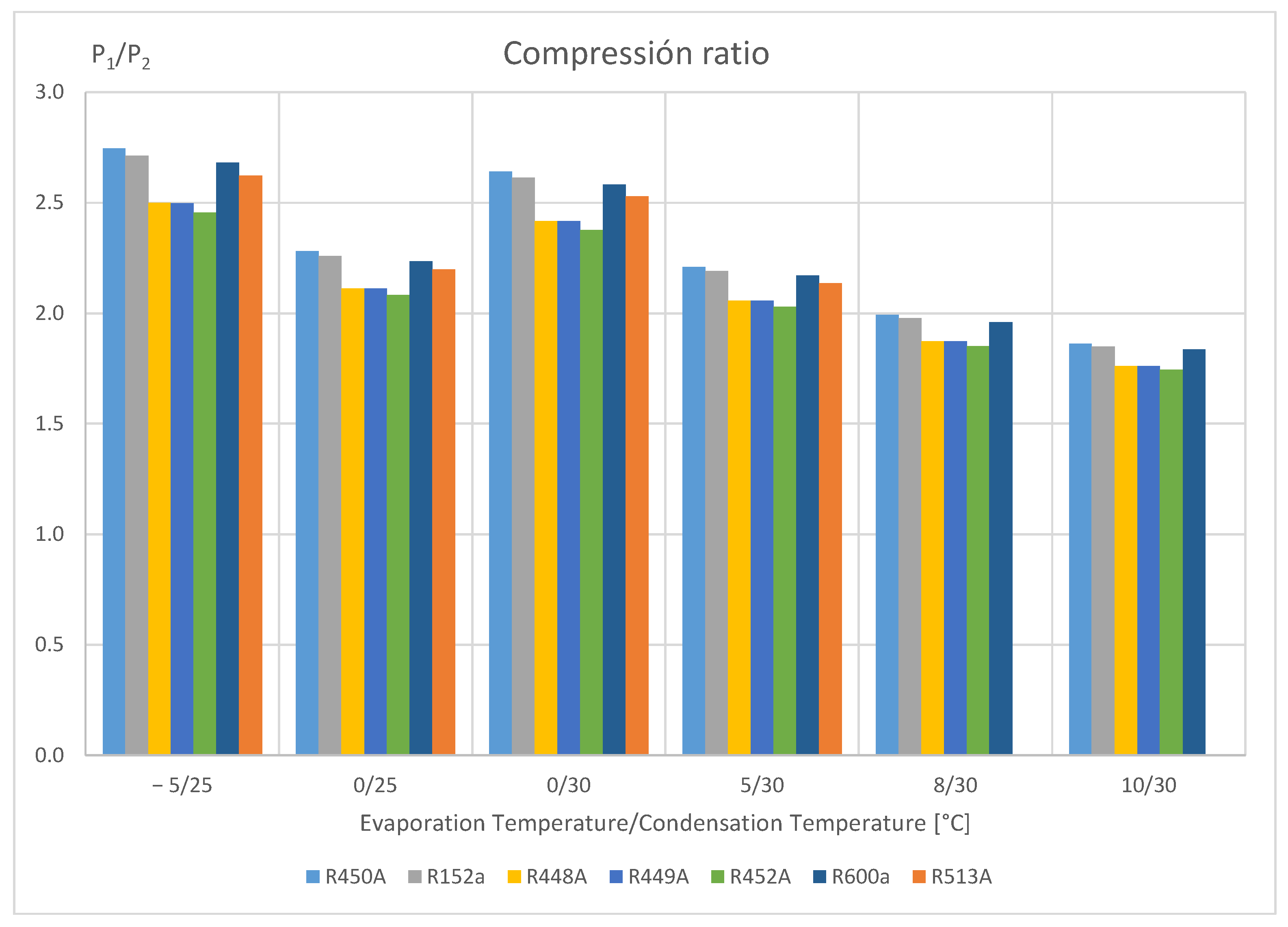
The values obtained from the compression ratio analysis for the different refrigerant and temperature combinations are shown below (Figure 4).

From Figure 5 it can be concluded that:

-

The compression ratios vary between 1.8 and 2.6 in average values. As expected, the maximum value (2.75) occurs at the highest temperature difference between evaporator and condenser, corresponding to R450A at operating temperatures of −5 °C/25 °C.

-

On the other hand, the minimum compression ratio is 1.74 (R452A for operating temperatures 10 °C/30 °C).

-

The behaviour of all substances is quite homogeneous, and the compression ratios can be ordered from lowest to highest as follows: R452A, R448A and R449A are practically the same to R513A, R600a, R152a, and R450A.

-

The fluids R152a and R600a, which have the best COP, have a similar compression ratio, although slightly lower in the case of R600a.

Similar to the previous section, the results for evaporator and condenser pressures (bar) for the different refrigerant and temperature combinations are presented below.

Analysing the results in

Table 6. Condenser and evaporator pressures for the different refrigerants.

Fluid	Condensation Temperature [°C]		Evaporation Temperature [°C]
	25	30	−5	0	5	8	10
R450A	5.85	6.77	2.13	2.56	3.07	3.40	3.64
R513A	7.14	8.22	2.72	3.25	3.85	-	-
R152a	5.97	6.91	2.20	2.64	3.15	3.49	3.73
R448A	12.03	13.76	4.81	5.69	6.69	7.35	7.81
R449A	11.90	13.61	4.76	5.63	6.62	7.27	7.73
R452A	12.50	14.26	5.09	6.00	7.03	7.70	8.18
R600a	3.50	4.05	1.31	1.57	1.86	2.06	2.20

, it can be seen that:

-

Again, the similar behaviour is maintained between the refrigerants R448A, R449A and R452A. They also have the highest pressure values.

-

As for the fluids R152a and R600a, both had a similar COP and compression ratio. However, the working pressures in the evaporator and condenser are lower in the case of R600a, which makes it a very interesting candidate when working in such small dimensions.

As a final comparison criterion, the compressor outlet temperature for the different refrigerant combinations, operating temperatures and compressor efficiencies are analysed below. For illustrative purposes, the graphs of the compressor outlet temperature as a function of its isentropic efficiency and the working fluid are shown, for the cases −5 °C/25 °C; 0 °C/25 °C and 0 °C/30 °C.

As can be seen in Figure 5, the trend observed in the rest of the criteria is repeated in terms of homogeneity between the different operating conditions. Quantitatively, the highest temperature values are reached by R448A, R449A and R152a. On the other hand, the lowest temperatures are reached by R600a, R513A and R450A, in that order. Of the seven refrigerant fluids analysed, the use of R448A, R449A and R452A can be ruled out, as they have the worst COP values in any possible working condition for the application of the project. The best COP values are obtained with R152a and R600a. Although both have very similar compression ratios, R600a works at lower pressures, which a priori makes it more interesting for the project and, above all, it has a lower outlet temperature in the compressor for the same operating conditions. The other two remaining fluids, R513a and R450a, have somewhat lower COP values, with compression ratios similar to R152a and R600a, although with higher working pressures than R600a.

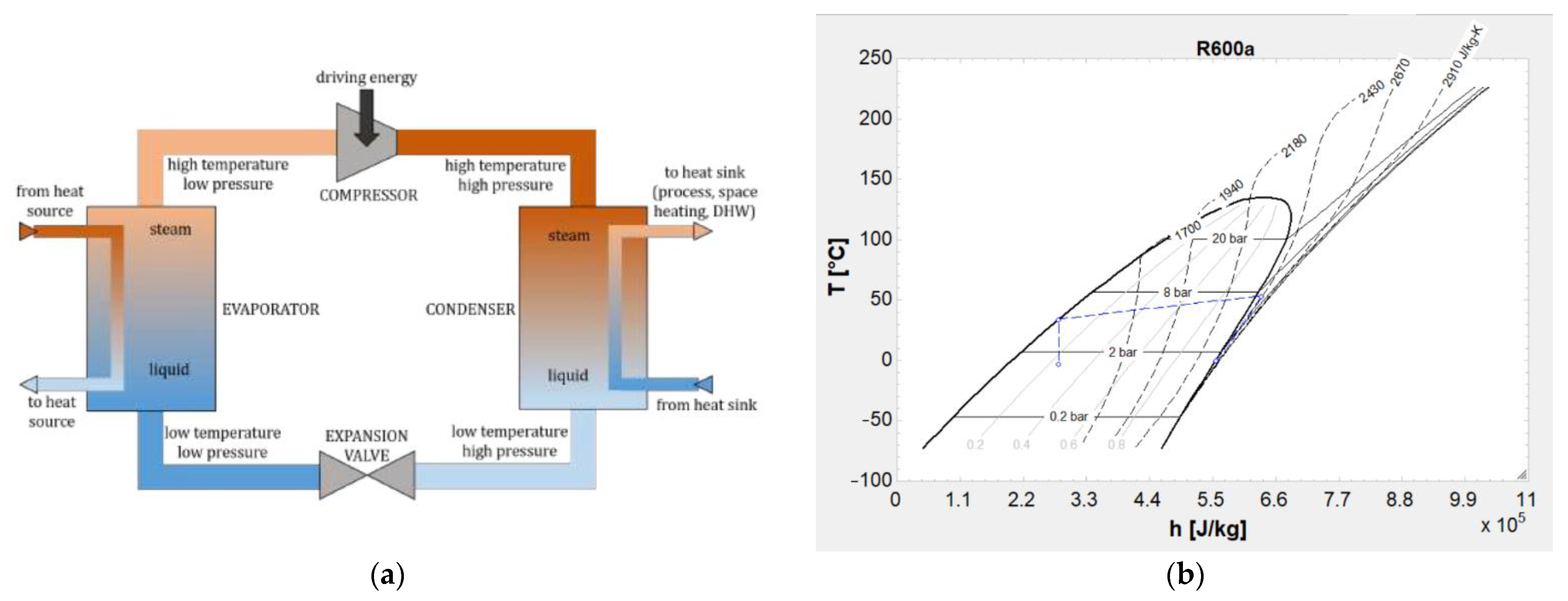
3.2. Design of the Model

As mentioned throughout the article, the work cycle to be carried out by the system is a vapour compression refrigeration cycle. This cycle has four main states that are developed at two specific pressures, high pressure (condenser) and low pressure (evaporator). The process starts at state 1, where the refrigerant is in a saturated vapour state or slightly superheated at low pressure. It then enters the compressor, where the refrigerant pressure rises to the high pressure (condenser), i.e., state 2. State 3 corresponds to the refrigerant in a saturated or slightly undercooled liquid state after passing through the condenser at constant pressure (pressure drop negligible). Finally, state 4 corresponds to the outlet of the lamination valve, where the refrigerant drops in pressure to a two-phase state prior to entering the evaporator. The cycle ends when the refrigerant travels through the evaporator at constant pressure (pressure drop negligible) to the saturated vapour state. The representation of the cycle can be seen in Figure 6.

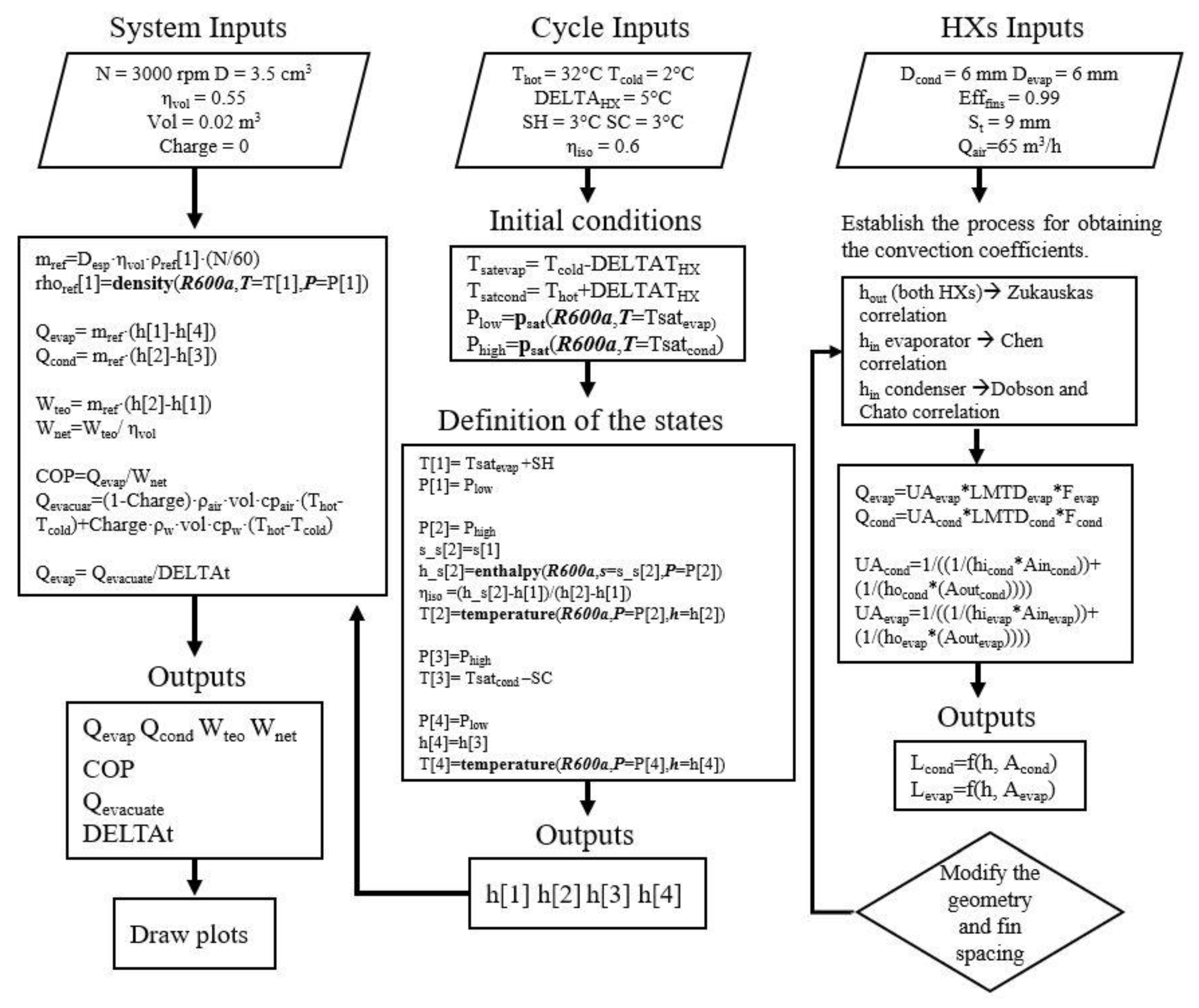
The model developed in EES (engineering equation solver) is based on a series of input data and calculation hypotheses, with the aim of defining the thermodynamic states at the inlet and outlet of each component, and, thus, calculate the refrigeration power or the COP of the cycle. Inputs include hot and cold source temperatures, compressor characteristics (displacement and rotational speed...) and some geometry data (tube diameter in heat exchangers, fin efficiency...). The assumption is that neither pressure drop nor heat losses are taken into account, nor the superheating and subcooling values near to the saturation curve.. The EES model is based on fundamental thermodynamic laws, and does not provide innovative information in the vapour compression cycle modelling. The operation of the model is explained below (Figure 7).

The flow diagram shows three blocks, the first one belongs to the mechanical part of the system, where the parameters belonging to the compressor can be configured. The second refers to the thermodynamic cycle, in this particular case the vapour compression refrigeration cycle. Finally, the third block introduces the parameters related to the heat exchangers of the system. In this block, the calculation of the convection coefficients is introduced so that, through the calculation of the global heat transfer coefficient, the lengths of the heat exchangers can be obtained.

As can be seen, the cycle block feeds the mechanical parameters block in order to obtain the heat and work as well as the COP, heat to be evacuated and the time required to do so. On the other hand, the exchanger block can be fed by new geometries in order to find the most interesting configurations.

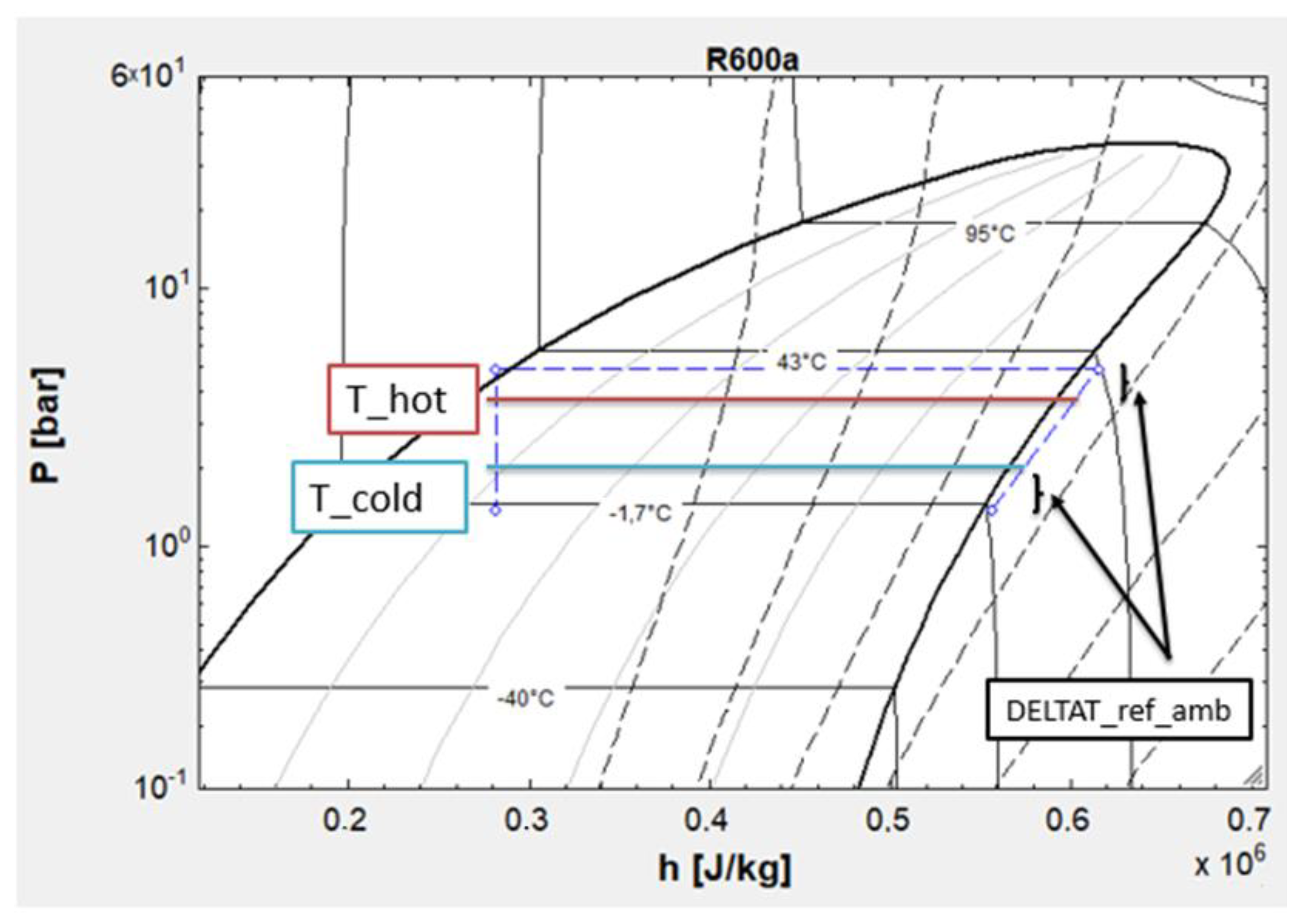
In order to characterize the process described, a series of inputs must be established that allow us to generate the model that describes the cycle by means of mathematical expressions. To begin with, it is necessary to know the temperature of the sources on which the cycle is to work. The hot reservoir corresponds to the temperature of the space in which the refrigeration system is located, and the temperature of the cold reservoir is the temperature inside the refrigeration system, i.e., the temperature to be reached. In order to be able to relate these parameters to the cycle, a new input DELTAT_ambref is introduced, this being the temperature difference that relates the aforementioned temperature of the heat sources with the refrigerant temperature in the hot source stage, corresponding to the condenser in the cycle, and the cold source, which corresponds to the evaporator.

It is common that, in this type of cycle, there are states of superheating and subcooling at the outlet of the evaporator and condenser, respectively. For this reason, these parameters have been introduced in our model to ensure that the refrigerant state is optimal: totally vapour in the case of the compressor inlet and totally liquid at the inlet of the lamination valve.

With the working temperatures established and knowing the state of the fluid at each point, the high and low pressures and the enthalpies (h_i) are known. The enthalpies determine the heat and work of the system as follows (Equations (1)–(4)):

$${\stackrel{·}{Q}}_{\mathit{cond}}=\stackrel{·}{m}·(h_2-h_3)$$

(1)

$${\stackrel{·}{Q}}_{\mathit{evap}}=\stackrel{·}{m}·(h_1-h_4)$$

(2)

$${\stackrel{·}{W}}_{{\mathit{comp}}_{\mathit{theo}}}=\stackrel{·}{m}·(h_1-h_2)$$

(3)

$${\stackrel{·}{W}}_{{\mathit{comp}}_{\mathit{real}}}={\stackrel{·}{W}}_{{\mathit{comp}}_{\mathit{theo}}} {\eta }_{\mathit{vol}}$$

(4)

where:

Q: the heat absorbed or received by the system (W);

$\stackrel{·}{m}$: the flow rate of refrigerant per unit time (kg/s);

h: enthalpy at each point in the cycle (J/kg);

$\stackrel{·}{W}$: work required by the system (W);

η_vol: volumetric efficiency of the compressor (-).

Leaving aside the parameters referring to the thermodynamic cycle, it is worth mentioning that it will also be necessary to take the variables describing the behaviour of the compressor as input. The equation relating the compressor operation to the duty cycle is as follows (Equation (5)):

$$\stackrel{·}{m}=D·{\eta }_{\mathit{vol}}·\frac{{\rho }_{\mathit{ref}}\ast N}{60}$$

(5)

where:

D: Compressor displacement (m³/rev);

ρ: density of the refrigerant in the inlet of the compressor (kg/m³);

N: revolutions of the compressor (rev/min).

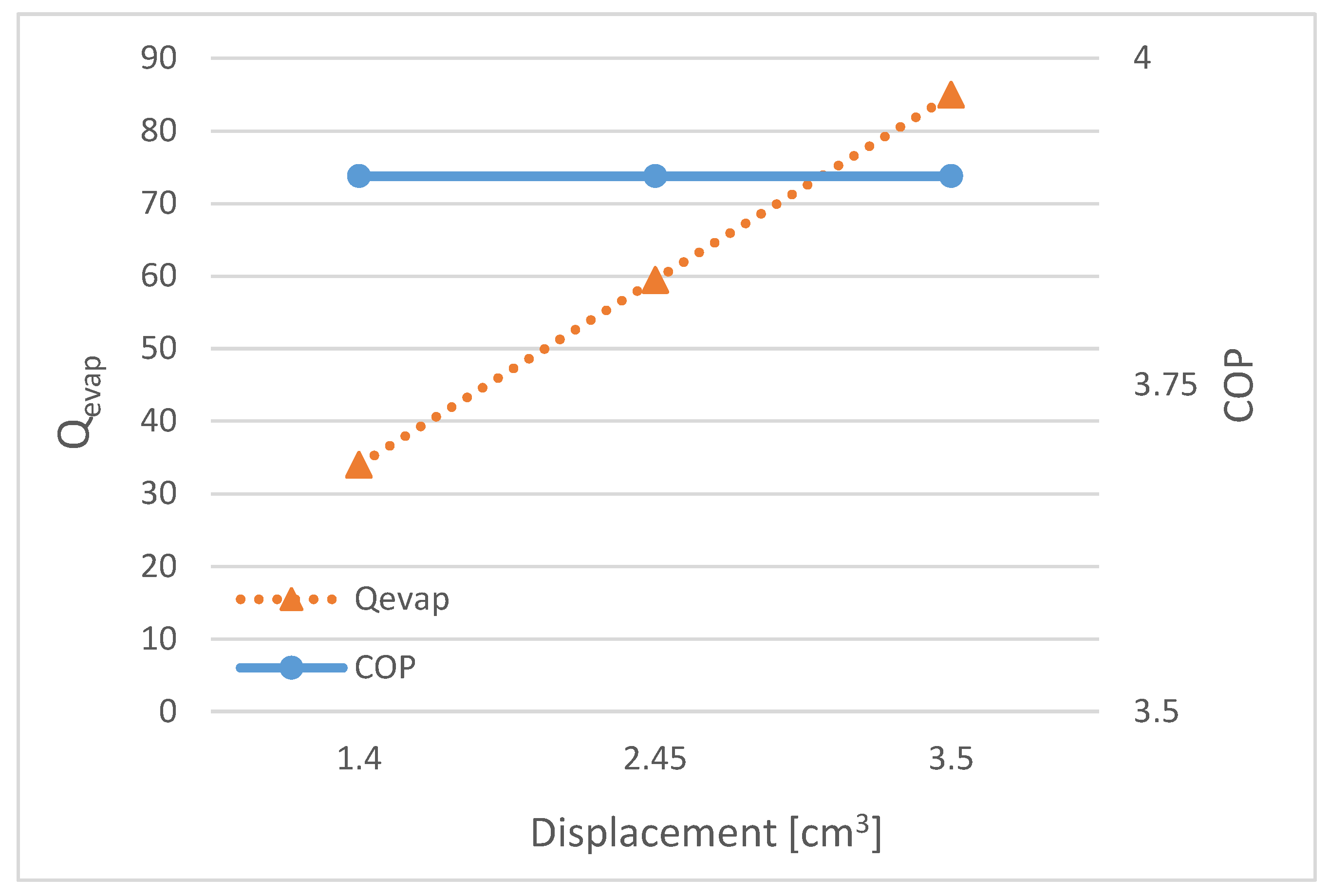
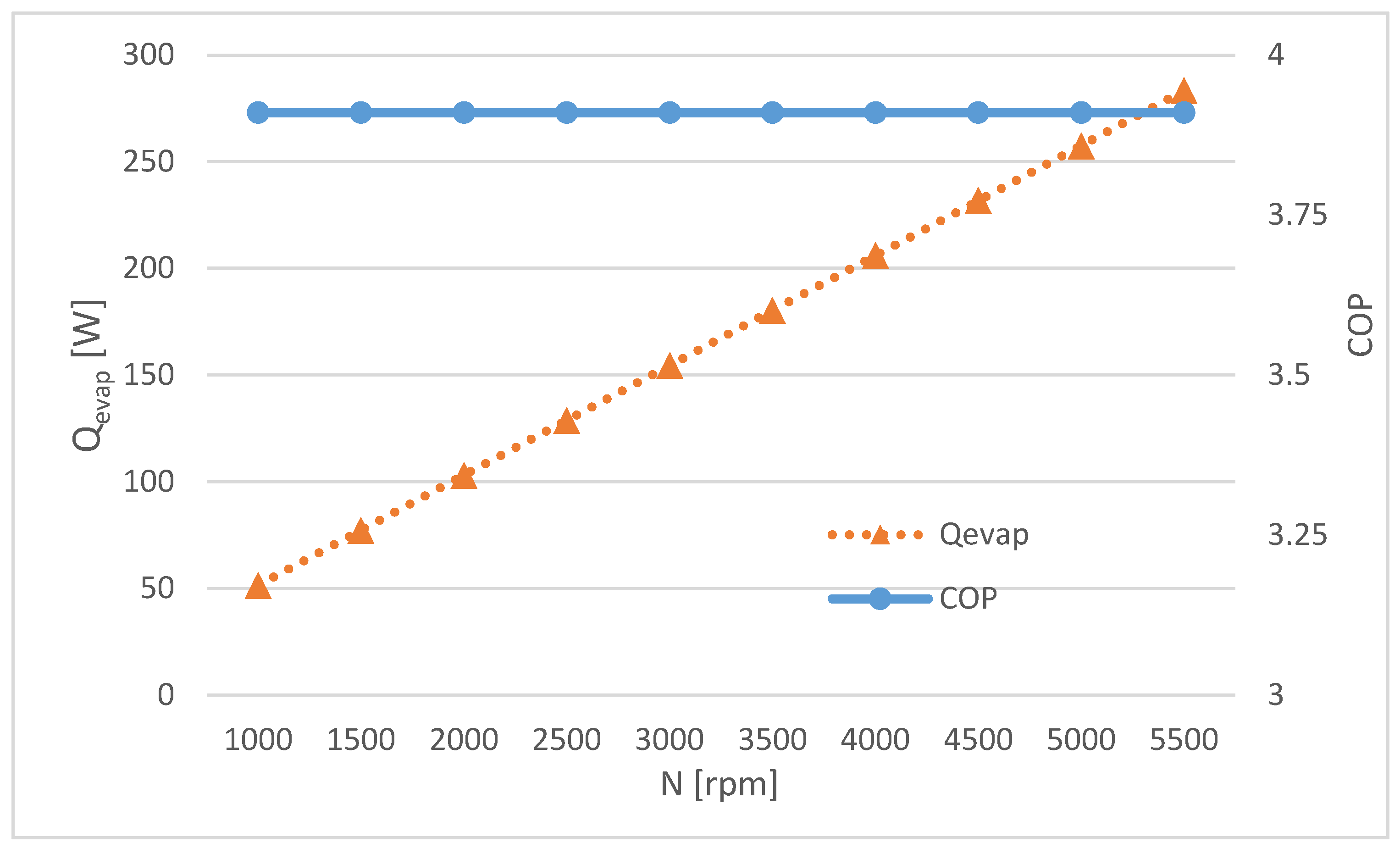
From the previous equation, the refrigerant mass flow rate is derived, a parameter that determines the cooling capacity of the system, as well as the work of the compressor. This parameter depends directly on the displacement (D), the volumetric efficiency of the compressor (η_vol), the density of the refrigerant (ρ_ref) at the inlet of the compressor and the revolutions (N). Of these variables, we keep the volumetric efficiency and density constant, while the displacement and rpm can be adjusted according to the objectives of the system.

With the mass flow rate of refrigerant through the system and the enthalpy at each point, we can obtain the work and heat of the system using the formulas described above.

The HXs, understood in this cycle as the condenser and evaporator, are key elements of the system. The design parameters in this case would be the overall heat transfer coefficient (U) and the exchange area (A). In order to carry out a preliminary study of the design of the exchangers, the heat to be extracted is determined from the setpoint temperatures, according to the following equation (Equation (6)):

$$\stackrel{·}{Q}=U·A·F·\mathit{LMTD}$$

(6)

where:

U: Total heat transfer coefficient (W/(m²·°C));

A: Area of the HX (m²);

F: Correction factor for crossflow HXs (-);

LMTD: Logarithmic mean temperature (°C).

Where the LMTD, the logarithmic mean temperature, is calculated as follows (Equation (7)):

$$\mathit{LMTD}=\frac{\Delta T_{\mathit{in}}-\Delta T_{\mathit{out}}}{\mathit{ln}\left(\frac{\Delta T_{\mathit{in}}}{\Delta T_{\mathit{out}}}\right)}$$

(7)

where ∆T_in is the temperature difference between the air and the refrigerant at the evaporator/condenser inlet and, likewise, ∆T_out is the temperature difference between the two fluids at the evaporator/condenser outlet. Since the HXs in this project are crossed HXs instead of counter flow HXs, it is necessary to apply a correction factor F to Equation (6). These temperatures are known, as well as the heat to be extracted or dissipated, so the only parameters that remain as unknowns are U and A, although they can be treated as a single unknown.

Once the UA parameter is solved from Equation (8), we can substitute it in the formula that relates this same parameter with the convective resistances (the conductive one is negligible), as well as with the heat exchange area (Equation (8)).

These convective resistances (h_in, h_out) refer to the convection coefficient both outside and inside the tube, in the same way that the transfer area is understood as the product of πDL, from which the necessary length of the exchangers can be obtained. In the case of the convection coefficients, both are considered forced; in the case of h_in because there is a fluid, the refrigerant, circulating through the circuit, and in the case of h_out because of the air generated by the fans towards the exchangers.

$$U=\frac{1}{\frac{1}{h_{\mathit{in}}·A_{\mathit{in}}}+\frac{ln\left(\frac{r_{\mathit{out}}}{r_{\mathit{in}}}\right)}{2·\pi ·k·L}+\frac{1}{h_{\mathit{out}}·A_{\mathit{out}}}}$$

(8)

The calculation of the value of the internal convective coefficient is given by such parameters as the tube diameter, the average fluid velocity, as well as its kinematic viscosity, density and conductivity evaluated at the average temperature of the fluid; and such dimensionless numbers as Reynolds, Prandtl and Nusselt. It is worth mentioning that the fluid is in a phase change zone, so it will be necessary to find a Nusselt correlation that considers this phenomenon. In the present development, use has been made of Chen’s correlation [30] (Equation (9)) for the evaporator, which calculates the effects of convective evaporation and nucleated evaporation separately. The value of Reynolds for the evaporator is 8603. In the case of the condenser, the phase change effect must also be taken into account, so the Dobson and Chato [31] (Equation (10)) correlation was used. For the condenser the value of Reynolds is 43.97.

$$\mathit{Nu}=0.023·{\mathit{Re}}^{\frac{4}{5}}·{\mathit{Pr}}^{0.4}$$

(9)

$$\mathit{Nu}=0.0195·{\mathit{Re}}^{0.8}·{\mathit{Pr}}^{0.4}·\sqrt{1.376+\left(\frac{C_a}{{X_{\mathit{tt}}}^{C_b}}\right)}$$

(10)

where:

Re: Reynolds number;

Pr: Prandlt number;

C_a: constant in Lockhart–Martinelli correlation;

X_tt: Martinelli Parameter;

C_b: constant in Lockhart–Martinelli correlation.

In the case of the external convective coefficient, for both HXs, the necessary variables for the calculation would be the air flow rate, the maximum velocity along the section, the diameter of the tubes, the viscosity of the fluid (air), its density and conductivity; and such dimensionless numbers as Reynolds, Prandtl and Nusselt. The Nusselt was obtained by means of Zukauska’s correlation [32] (Equation (11)). The Reynolds values for the condenser and evaporator are 6087 and 4640, respectively. Therefore, the values for the correlation constants will be between the Reynolds range 1000–2 · 10⁵: being c = 0.27; m = 0.63; and n = 0.36.

$$\mathit{Nu}=0.27·{\mathit{Re}}^{0.63}·{\mathit{Pr}}^{0.36}·{\left(\frac{\mathit{Pr}}{{\mathit{Pr}}_s}\right)}^{0.25}$$

(11)

where:

Re: Renoys number;

Pr: Prandlt number;

Pr_s: Prandlt number calculated at the surface temperature.

With all the parameters, the value of the convection coefficients, both external and internal, are found from the same formula (Equation (12)). In this study, the diameter of the tube was fixed in 6 mm.

$$\mathit{Nu}=\frac{h_{\mathit{in}}·D}{k}$$

(12)

where:

D: diameter of the tube (m);

k: thermal conductivity of the fluid (W/(m·°C)).

As far as the lamination valve is concerned, it has been modelled as a capillary tube, where the fluid will pass with constant enthalpy from one pressure to another due to the pressure drop when passing through a tube with a very small diameter.

With regard to the validation of the model, the study carried out by Ozsipahi et al. [33] has been used as a reference, where the behaviour of different refrigerants, including R600a, at different compressor speeds was studied. The parameters that have been introduced as inputs for our model are the evaporation/condensation temperature, the superheating and subcooling and the isentropic and volumetric efficiency of the compressor. Based on these data, the study carries out tests at different speeds, of which the results obtained at 1500, 2100 and 3000 rpm have been taken as a reference to compare, as this is the speed range used in this project.

Table 7. Validation data.

		Compression Ratio (CR)			${\displaystyle \stackrel{\mathbf{·}}{\mathit{m}}}$ (g/s)			${\displaystyle \stackrel{\mathbf{·}}{\mathit{W}}}$ (W)–Input Power			COP
Case	n (rpm)	Reference	Model	Error	Reference	Model	Error	Reference	Model	Error	Reference	Model	Error
1	1500	11.5	11.9	−3.2%	0.28	0.27	4.9%	52.9	50.8	3.9%	1.78	1.79	−0.6%
2	2100	11.8	11.9	−0.8%	0.39	0.38	2.5%	72.8	71.1	2.3%	1.81	1.80	0.7%
3	3000	12.5	11.7	6.3%	0.52	0.55	−4.9%	101.3	103.1	−1.8%	1.70	1.75	−2.9%

shows the results obtained as well as the error.

4. Results

For the cases to be presented below, the following values shown in

Table 8. Input data for the numerical model.

Thot	Tcold	DELTATambref	SC	SH	N	D	ηvol	Stock
32 °C	2 °C	5 °C	3 °C	3 °C	1650 rev/min	3.5 cm3	0.85	0

have been taken as input values:

T_hot and T_cold are the design temperatures corresponding to the hot and cold sources of the cycle, i.e., to the temperature of the air from which it starts (32 °C) to cool to the setpoint temperature of the refrigerator (2 °C). DELTAT_ambref is the temperature difference that relates the above mentioned difference between the temperature of the heat sources and the refrigerant in the hot source stage, corresponding to the condenser in the cycle, and the cold source, which corresponds to the evaporator. The parameters SH (super heating) and SC (sub cooling) refer to the temperature increase at the evaporator outlet and the temperature decrease at the condenser outlet with respect to the saturation temperature.

The first parametric analysis is the influence of the displacement on the COP of the system. From Figure 8 it can be seen that, although the COP does not vary as the ratio increases proportionally, the cooling capacity increases considerably with the displacement. Therefore, the conclusion to be drawn is that it is more convenient to work with displacements close to 3.5 cm³, a value that has been observed to be achievable for compact systems.

Compressor speed is another parameter to be analysed. In the same way as the displacement, and as can be seen in the formula previously presented, the compressor revolutions increase the circulation flow rate. This translates into an increase in both the cooling power and the power consumed by the compressor, while the COP remains constant. The parametric study of the optimum compressor speed is intended to provide an answer to the question of what the optimum speed range would be for cooling the required power. We can see the parametric study in Figure 9.

Figure 9 shows that, for the cooling power required for this type of cycle (around 100 W), the speed value will be around 2000 rpm. It should be noted that this value is independent of the system load; the only parameter that will be altered as the load increases is the time required by the system to evacuate the heat from it, so it can be concluded that the compressor will be set at a constant speed.

With regard to the volumetric efficiency of the compressor, it is logical that the higher the efficiency, the better the results obtained in terms of COP. For the simulations, a volumetric efficiency of 0.85 has been taken according to the literature consulted. However, this value will be reduced due to the scalability of the system.

In reality, the volumetric efficiency values will be around 0.5–0.6, which will not only lower the COP, but also the cooling capacity of the cycle. Therefore, in order to obtain the desired 100 W, the compressor speed will have to be adjusted.

Table 9. Compressor speed required to obtain the same cooling capacity for different volumetric efficiencies.

ηvolumetric	N [rev/min]	Qevap [W]	COP
0.5	3500	106	2.3
0.6	3000	109.1	2.76
0.7	2500	106	3.22
0.8	2100	101.8	3.68
0.9	1900	103.6	4.14

shows the tests that were carried out by varying the volumetric efficiency and, in turn, adjusting the revolutions in order to obtain this power. We can also observe the effect of varying the volumetric efficiency on the COP.

It is important to know the influence of the load on the reaction of the cycle to different work requirements. The mini fridge we are working with has a volume of 20 L; thanks to the equation presented below, we can include the filling percentage of the fridge (Equation (13)).

$$Q_{\mathit{evap}}=(1-\mathit{storage})·c_{p-\mathit{air}}·{\rho }_{\mathit{air}}·\mathit{vol}·(T_{\mathit{hot}}-T_{\mathit{cold}})+\mathit{storage}·c_{p-\mathit{w}}·{\rho }_{\mathit{w}}·\mathit{vol}·(T_{\mathit{hot}}-T_{\mathit{cold}})$$

(13)

where:

Storage: the fraction of space occupied in the fridge by beverages (-);

C_p−air: calorific value of air (kJ/kg·°C);

c_p−w: calorific value of the water (kJ/kg·°C);

ρ_air: density of the air (kg/m³);

ρ_w: density of the water (kg/m³);

vol: volume of the fridge (m³);

T_hot: temperature of the hot reservoir (°C);

T_cold: temperature of the cold reservoir (°C).

The first part of the formula expresses the percentage of air in the volume, while the second part corresponds to water (liquid, in any case). From this expression (Equation (14)), we obtain the necessary heat to be extracted to cool the volume from an initial temperature to the refrigerator’s set point temperature. On the other hand, the heat to be evacuated in terms of power (W) corresponds to the heat that the system is capable of extracting according to the thermodynamic cycle. Once the necessary heat to be extracted and the heat that the cycle is capable of extracting are known, the time that would be needed to carry out this cooling can also be known.

$${\stackrel{·}{Q}}_{\mathit{evap}}\left(\mathrm{W}\right)=\frac{Q_{\mathit{evap}}}{t}$$

(14)

Figure 10 shows that, as the load increases, the heat to be extracted for cooling from a high temperature to a low temperature also increases, and, as is logical, the time required to carry out this exchange also increases. In the case of full load, and for the designed temperatures (from 32 °C to 2 °C), the maximum time required to achieve the specifications is 8.2 h.

In the previous section, we have shown the different proposals made by other studies. For our project, we have opted for a bank of tubes where the length is calculated by means of the numerical process described in the methodology. After carrying out these calculations, tube lengths were too long, so it was decided to add fins to the model. The fins are transversal to the tubes and occupy the exchanger section itself.

The recalculation of the necessary exchange surface and therefore the length of the tubes is made according to the combination of three factors: the cooling capacity, the cross-section of the exchanger and the fin spacing. Since the size of the fins depends on the HX cross-section, the calculation process is iterative. In

Table 10. Exchanger dimensions according to power requirement, HX cross-section and fin spacing.

Power	Section	Fin Separation	Minimum Depth Evaporator	Minimum Depth Condenser	Length Evaporator	Length Condenser
100 W	40 × 40 mm	1.5 mm	54 mm	45 mm	0.37 m	0.64 m
		3 mm	81 mm	63 mm	0.82 m	0.85 m
		5 mm	108 mm	81 mm	1.76 m	1.12 m
	60 × 60 mm	1.5 mm	44 mm	35 mm	0.63 m	1.07 m
		3 mm	63 mm	45 mm	1.88 m	1.26 m
		5 mm	85 mm	54 mm	3.15 m	1.92 m

, the different combinations can be seen.

5. Discussion and Conclusions

This project aimed to delve into the niche market of compact refrigeration equipment. During the process, research was carried out on the current state of the art in order to obtain the guidelines outlining the methodology of the current project. After carrying out the model in EES and parameterizing the most influential variables, different conclusions can be drawn:

• The compressor is the heart of the system. The correct configuration of the compressor determines the behaviour of the equipment. Although there will be parameters, such as volumetric efficiency, that do not depend on us, we have to control others, such as the relationship between displacement and revolutions, as this is crucial to obtaining the desired cooling capacity.
• The COP is mainly affected by the volumetric efficiency of the compressor, so at low efficiency, we have to increase the revolutions to obtain a specific power. For this reason, it was concluded that it would be better to keep the displacement values at around 3.5 cm³ (existing compressor on the market) in order to have a greater margin to increase the speed of the compressor without going to high speeds.
• The design of the HXs is also of great relevance in such compact equipment; the influence of the HXs can vary the performance. In the review of the state of the art, it was concluded that the most commonly used type of exchanger is the thin plate, with or without fins.
• Due to the fact that we are looking for a relatively high power, 100 W, and to maintain a competitive COP, it is definitely necessary in our project for the exchangers to have fins in both cases.
• Another study, parallel to the thermodynamic cycle, was the choice of the optimum refrigerant. After analysing several different cases, it was concluded that the refrigerant R600a shows favourable characteristics for working in such systems as the present one.

Therefore, based on the conclusions obtained, we can say that this is a challenging case and that the search for reduced dimensions in this type of system is an objective that depends on different variables. However, the existence of similar equipment and the current modelling techniques do not make it an impossible goal.

References

1. Chua, K.J.; Chou, S.K.; Yang, W.M.; Yan, J. Achieving Better Energy-Efficient Air Conditioning—A Review of Technologies and Strategies. Appl. Energy 2013, 104, 87–104. [Google Scholar] [CrossRef]
2. Ham, S.W.; Kim, M.-H.; Choi, B.-N.; Jeong, J.-W. Energy saving potential of various air-side economizers in a modular data center. Appl. Energy 2015, 138, 258–275. [Google Scholar] [CrossRef]
3. Heinloth, K. Energy Technologies. In Renewable Energy; Springer: Berlin/Heidelberg, Germany, 2006. [Google Scholar]
4. Barbosa, J.R., Jr.; Ribeiro, G.B.; de Oliveira, P.A. A State-of-the-Art Review of Compact Vapor Compression Refrigeration Systems and their Applications. Heat Transf. Eng. 2012, 33, 356–374. [Google Scholar] [CrossRef]
5. Alalaimi, M.; Lorente, S.; Anderson, R.; Bejan, A. Effect of size on ground-coupled heat pump performance. Int. J. Heat Mass Transf. 2013, 64, 115–121. [Google Scholar] [CrossRef] [Green Version]
6. Heppner, J.D.; Walther, D.C.; Pisano, A.P. ARCTIC: A Rotary Compressor Thermally Insulated µCooler. ASME Int. Mech. Eng. Congr. Expo. 2005, 4224, 287–294. [Google Scholar] [CrossRef]
7. Chiriac, V.; Chiriac, F. An Alternative Method for the Cooling of Power Microelectronics Using Classical Refrigeration. J. Electron. Packag. 2008, 130, 041103. [Google Scholar] [CrossRef]
8. Mancin, S.; Zilio, C.; Righetti, G.; Rossetto, L. Mini Vapour Cycle System for High Density Electronic Cooling Applications. Int. J. Refrig. 2012, 36, 1191–1202. [Google Scholar] [CrossRef]
9. Mongia, R.; Masahiro, K.; DiStefano, E.; Barry, J.; Chen, W.; Izenson, M.; Possamai, F.; Zimmermann, A.; Mochizuki, M. Small scale refrigeration system for electronics cooling within a notebook computer. In Proceedings of the Thermal and Thermomechanical Proceedings 10th Intersociety Conference on Phenomena in Electronics Systems, San Diego, CA, USA, 30 May–2 June 2006. [Google Scholar] [CrossRef]
10. Sung, T.; Lee, D.; Kim, H.S.; Kim, J. Development of a novel meso-scale vapor compression refrigeration system (mVCRS). Appl. Therm. Eng. 2014, 66, 453–463. [Google Scholar] [CrossRef]
11. Trutassanawin, S.; Groll, E.; Garimella, S.; Cremaschi, L. Experimental Investigation of a Miniature-Scale Refrigeration System for Electronics Cooling. IEEE Trans. Compon. Packag. Technol. 2006, 29, 678–687. [Google Scholar] [CrossRef] [Green Version]
12. Maveety, J.G.; Chrysler, G.M.; Sanchez, E.A.; Brown, M.F.W. Thermal Management for Electronics Cooling using a Miniature Compressor. Proc. Int. Microelectron. Packag. Soc. (IMAPS) 2002, 33, 356–374. [Google Scholar]
13. Chang, C.-C.; Liang, N.-W.; Chen, S.-L. Miniature Vapor Compressor Refrigeration System for Electronic Cooling. IEEE Trans. Compon. Packag. Technol. 2011, 33, 794–800. [Google Scholar] [CrossRef]
14. Poachaiyapoom, A.; Leardkun, R.; Mounkong, J.; Wongwises, S. Miniature vapor compression refrigeration system for electronics cooling. Case Stud. Therm. Eng. 2019, 13, 100365. [Google Scholar] [CrossRef]
15. Ma, R.; Wu, Y.-T.; Du, C.-X.; Chen, X.; Zhang, D.-L.; Ma, C.-F. The performance test of a modified miniature rotary compressor in upright and inverted modes subjected to microgravity. Appl. Therm. Eng. 2016, 92, 81–92. [Google Scholar] [CrossRef]
16. Carter, H., III; Chow, L.; Kapat, J.; Laveau, A.; Sundaram, K.; Vaidya, J. Component Fabrication and Testing for a Meso-Scale Refrigerator; American Institute of Aeronautics and Astronautics: Albuquerque, NM, USA, 1999. [Google Scholar]
17. Shannon, M.A.; Philpott, M.L.; Miller, N.R.; Bullard, C.W.; Beebe, D.J.; Jacobi, A.M.; Hrnjak, P.S.; Saif, T.; Aluru, N.; Sehitoglu, H.; et al. Integrated Mesoscopic Cooler Circuits (IMCCs). In Proceedings of the ASME International Mechanical Engineering Congress and Exposition, Nashville, TN, USA, 14–19 November 1999; American Society of Mechanical Engineers: New York, NY, USA, 1999; pp. 75–82. [Google Scholar] [CrossRef]
18. Hao, Z.; Kapat, J.S.; Chow, L.C.; Sundaram, K.B. Design and Analysis of a Miniature Reciprocating Compressor Driven by a Comb Drive. Proc. ASME Intl. Eng. Congr. Expo. 2000, 40, 111–118. [Google Scholar] [CrossRef]
19. Bash, C.; Patel, C.; Beitelmal, A. Acoustic compression for the thermal management of multi-load electronic systems. In Proceedings of the ITherm 2002 Eighth Intersociety Conference on Thermal and Thermomechanical Phenomena in Electronic Systems, San Diego, CA, USA, 30 May–1 June 2002. [Google Scholar] [CrossRef]
20. Unger, R.; Novotny, S. A High-Performance Linear Compressor for CPU Cooling; Purdue University: West Lafayette, Indiana, 2002. [Google Scholar]
21. Sathe, A.; Groll, E.; Garimella, S. Experimental Evaluation of a Miniature Rotary Compressor for Application in Electronics Cooling; Purdue University: West Lafayette, Indiana, 2008. [Google Scholar]
22. Ernst, T.C.; Garimella, S. Wearable Engine-Driven Vapor-Compression Cooling System for Elevated Ambients. J. Therm. Sci. Eng. Appl. 2009, 1, 025001. [Google Scholar] [CrossRef]
23. Sathe, A.A.; Groll, E.A.; Garimella, S.V. Dynamic analysis of an electrostatic compressor. Int. J. Refrig. 2010, 33, 889–896. [Google Scholar] [CrossRef] [Green Version]
24. Wu, Y.; Ma, C.-F.; Zhong, X.-H. Development and experimental investigation of a miniature-scale refrigeration system. Energy Convers. Manag. 2010, 51, 81–88. [Google Scholar] [CrossRef]
25. Bradshaw, C.R.; Groll, E.A.; Garimella, S.V. A comprehensive model of a miniature-scale linear compressor for electronics cooling. Int. J. Refrig. 2011, 34, 63–73. [Google Scholar] [CrossRef] [Green Version]
26. Yee, R.P.; Hermes, C.J. Thermodynamic design of a mesoscale vapor compression cooling device. Appl. Therm. Eng. 2019, 147, 509–520. [Google Scholar] [CrossRef] [Green Version]
27. Babarinde, T.O.; Akinlabi, S.; Madyira, D.M.; Ohunakin, O.; Adelekan, D.S.; Oyedepo, S.O. Comparative Analysis of the Exergetic Performance of a Household Refrigerator Using R134a And R600a. Int. J. Energy Clean Environ. 2018, 19, 37–48. [Google Scholar] [CrossRef] [Green Version]
28. Wu, Z.; Du, R. Design and Experimental Study of a Miniature Vapor Compression Refrigeration System for Electronics Cooling. Appl. Therm. Eng. 2011, 31, 385–390. [Google Scholar] [CrossRef]
29. Wisconsin-Madison University. EES Engineering Equation Solver. Available online: https://fchartsoftware.com/ees/index.php/ (accessed on 15 April 2021).
30. Juan, H.C.; Armando, G.M.; Juan Manuel, B.F. Análisis de la Transferencia de Calor en un Evaporador Utilizando Diferentes Refrigerantes; Memorias del XXVII Congreso Nacional de Termodinámica: Toluca, México, 2012. [Google Scholar]
31. Boissieux, X.; Heikal, M.; Johns, R. Two-phase heat transfer coefficients of three HFC refrigerants inside a horizontal smooth tube, part II: Condensation. Int. J. Refrig. 2000, 23, 345–352. [Google Scholar] [CrossRef]
32. Žukauskas, A. Heat Transfer from Tubes in Crossflow. Adv. Heat Transf. 1972, 8, 93–160. [Google Scholar] [CrossRef]
33. Ozsipahi, M.; Kose, H.A.; Kerpicci, H.; Gunes, H. Experimental Study of R290/R600a Mixtures in Vapor Compression Refrigeration System. Int. J. Refrig. 2022, 133, 247–258. [Google Scholar] [CrossRef]
Figure 1. Vapour compression cycle: (a) scheme with the main components; (b) t-h diagram for the R600 fluid.
Energies 15 00819 g001
Figure 2. Design of heat exchangers.
Energies 15 00819 g002
Figure 3. COP values as a function of the isentropic efficiency for the cases: (a) 0 °C/30 °C; (b) 0 °C/25 °C; (c) −5 °C/25 °C.
Energies 15 00819 g003
Figure 4. Compression ratio analysis for the different refrigerant and temperature combinations.
Energies 15 00819 g004
Figure 5. Compressor outlet temperature for the different refrigerants (a) 0 °C/30 °C (b) 0 °C/25 °C (c) −5 °C/25 °C.
Energies 15 00819 g005
Figure 6. Refrigeration cycle on EES.
Energies 15 00819 g006
Figure 7. Flow chart of the programme in EES.
Energies 15 00819 g007
Figure 8. Influence of the displacement on the COP.
Energies 15 00819 g008
Figure 9. Influence of the compressor speed on the COP.
Energies 15 00819 g009
Figure 10. Time taken by the system to dissipate heat according to stock.
Energies 15 00819 g010