Geological Characterization of the 3D Seismic Record within the Gas Bearing Upper Miocene Sediments in the Northern Part of the Bjelovar Subdepression—Application of Amplitude Versus Offset Analysis and Artificial Neural Network

Abstract

As natural gas reserves are generally decreasing there is a need to successfully characterize potential research objects using geophysical data. Presented is a study of amplitude vs. offset, attribute and artificial neural network analysis on a research area of a small gas field with one well with commercial accumulations and two wells with only gas shows. The purpose of the research is to aid in future well planning and to distinguish the geophysical data in dry well areas with those from an economically viable well. The amplitude vs. offset analysis shows the lack of anomaly in the wells with only gas shows while the anomaly is present in the economically viable well. The artificial neural network analysis did not aid in the process of distinguishing the possible gas accumulation but it can point out the sedimentological and structural elements within the seismic volume.

1. Introduction

With a general decrease in the recoverable reserves of natural gas both onshore [1] and offshore [2], the need to locate new accumulations is more than evident. Exploration for hydrocarbon reservoirs relies on a very large number of input data for characterization of the subsurface. This work focuses on usage of attribute analysis on seismic volume, amplitude versus offset (AVO) analysis as well as searching for patterns within many extracted seismic attributes by self-organizing artificial neural networks (SOANNs). The seismic amplitude versus offset (AVO) analysis has become prominent as the direct hydrocarbon indicator in the last decade, aimed at characterizing the fluid content or the lithology of a possible reservoir and reducing the exploration drilling risk [3].

Seismic attribute analysis was performed on reprocessed and reinterpreted seismic volumes. Progress in characterization of hydrocarbon reservoirs is enabled by the analysis of seismic attributes. In saturated gas reservoirs the character of seismic signals changes. Results of the seismic attribute analysis indicate prospectives east and southeast from the discovered field. For the analysis of interception and gradient as primary AVO attributes, pre-stack data or common depth point (CDP) gathers data used by the method of summing traces from common depth points in the subsurface. Obtained crossplot of intercept and gradient can determine the appropriate AVO class that shows changes in amplitude relative to the offset.

SOANNs were used on the same dataset as the seismic attribute analysis which were extracted on the top of the targeted seismic horizon. Patterns indicate mostly sedimentological features that can be tied to the variability of the depositional environment.

2. Materials and Methods

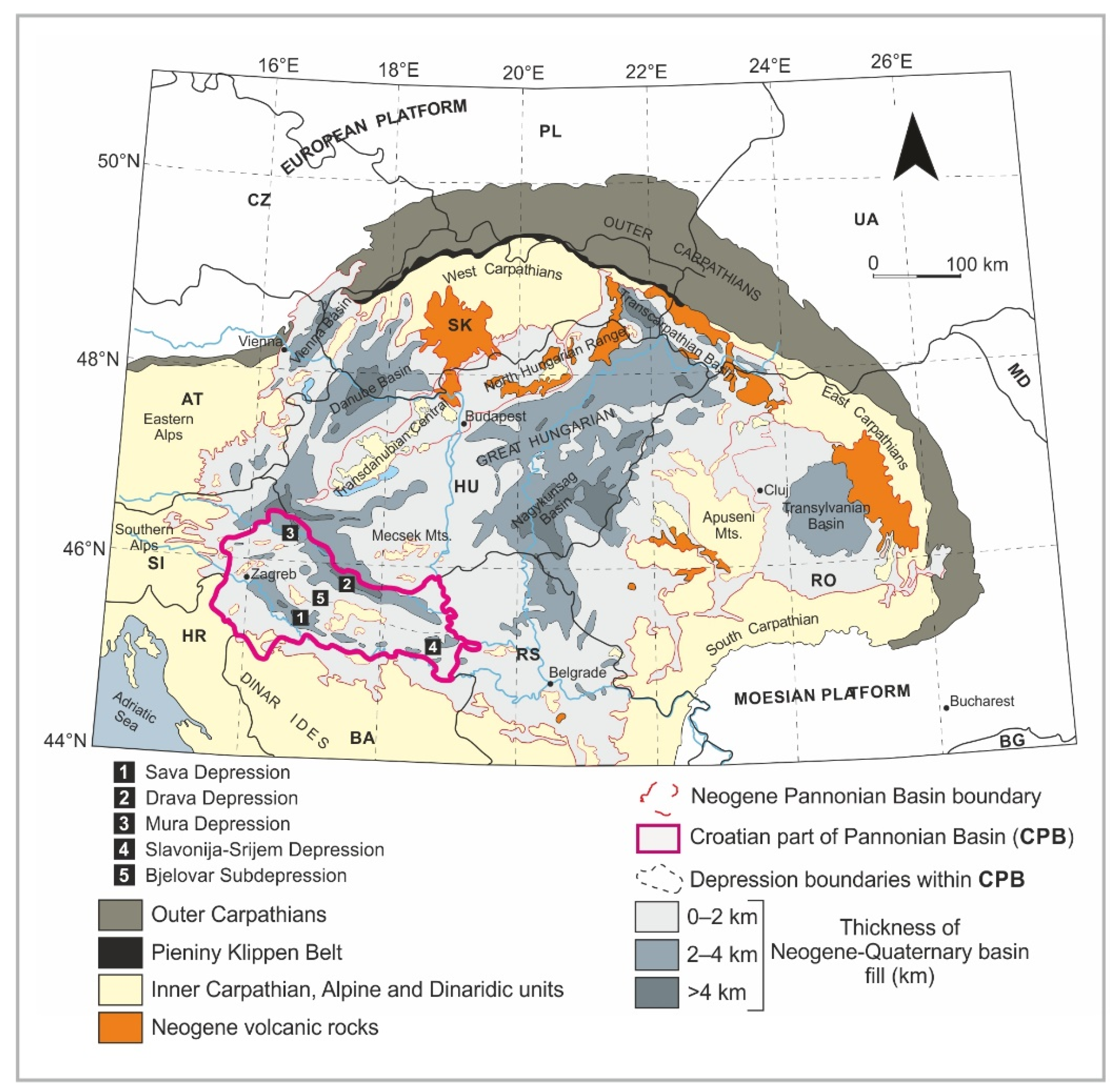
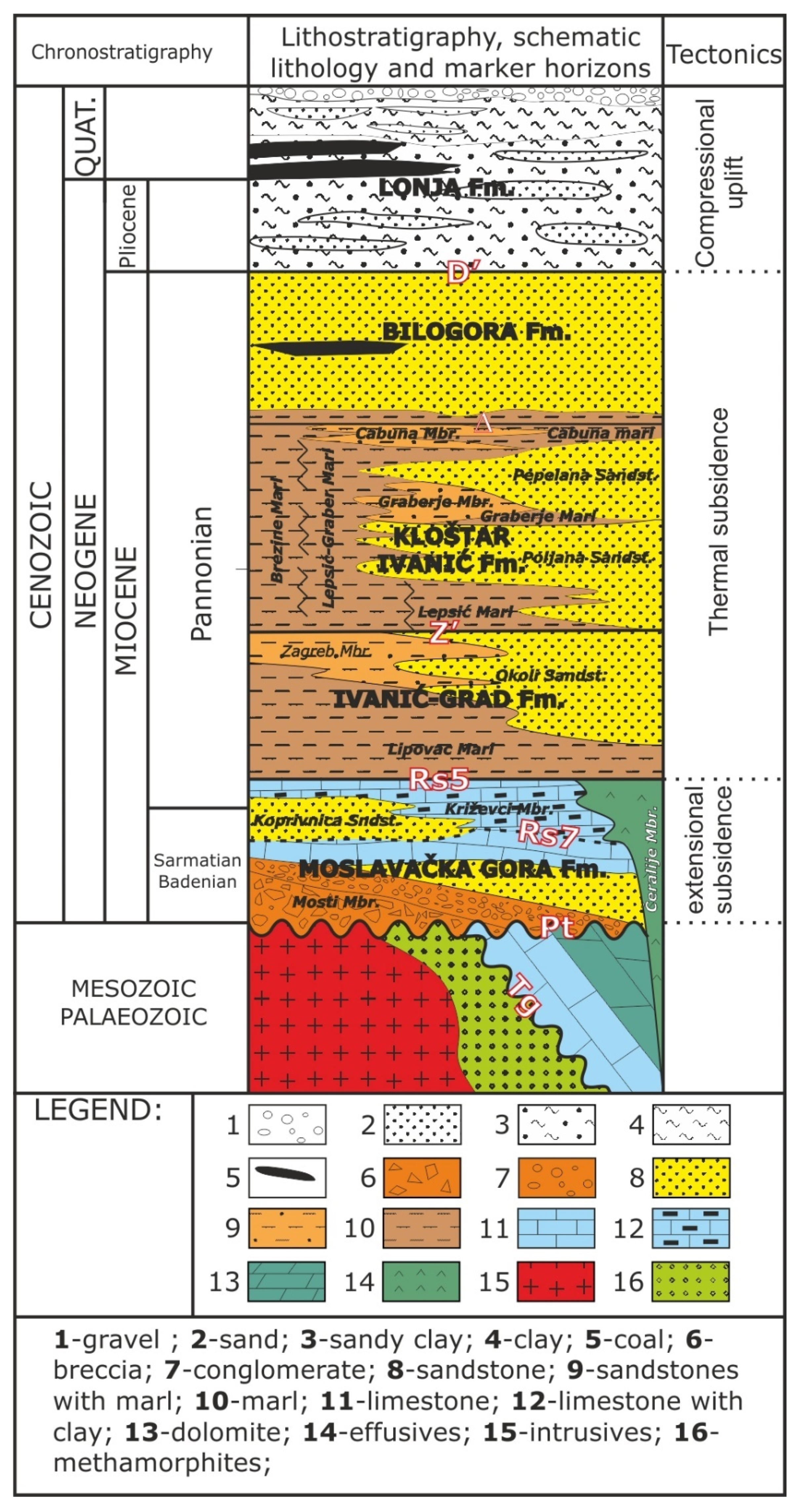
2.1. Geological Settings of the Exploration Area

The Bjelovar Subdepression is located in the Croatian part of the Pannonian Basin (CPB), within the southwestern part of the Drava Depression (Figure 1). The total area of Drava Depression is approximately 12,000 km², of which 9100 km² is within the Republic of Croatia [4]. Geographically, it is surrounded by the Kalnik Mountain in the northwest, Bilogora Mountain in the northeast, Papuk Mountain, Ravna Gora Mountain and Psunj Mountain in the east and Moslavačka Gora Mountain in the south.

The total thickness of the Neogene and Quaternary deposits can be more than 7000 m in the middle part of the Drava Depression while in the Bjelovar Subdepression it can reach up to 3500 m thickness [5]. The analyzed gas field is located on the edge of the Bjelovar Subdepression (Figure 1) near the boundary with the Drava Depression (Croatian part of the Pannonian Basin System, CPBS). Three wells were drilled on the structure: Well-1, Well-2 and Well-3.

The formation of the Pannonian Basin System (PBS) began in Early Miocene when the Eurasian plate began to subduct under the Pannonian crustal fragment [8]. Numerous local transtensions as proto-areas of later depressions and subdepressions opened between the southern and northern boundaries of the PBS ([9,10]). The Croatian part of the PB (CPB) structural complex can be subdivided into three major megacycles [8,10] in relation to dominant tectonic events (Figure 2).

Major structural depressions, in the Croatian part of the Pannonian Basin are the Mura, Drava, Sava and Slavonija-Srijem depressions. The Bjelovar Subdepression is a part of the Drava Depression. Lithostratigraphy and regional geological relations are described in detail by several authors [8,11,12]. The focus of this research is located within Bilogora Fm. between well log markers Δ and D’ (Reservoir 1) and Reservoir 2 is located within Pepelana sandstones between well log markers Z and Δ (Figure 2).

2.2. Input Data

Seismic data reprocessing was done using up to date processing techniques and ended with Kirchhoff pre-stack time migration (PSTM, Figure 3a) flow. The input seismic data to the Kirchhoff pre-stack depth migration (PSDM) was the same set as for the time migration. The final pre-stack depth migration image resulted in better representation of the subsurface structures and stratigraphy, enabling greater interpretation confidence especially in the area of low signal to noise ratio.

PSDM shows enhancement in the image of the prospective area indicating anomalies present on the structural trap closure. Reliable and detailed analysis of thin deposits can only be performed on reprocessed and reinterpreted 3D volumes (Figure 3b). Location of the seismic section and structural maps of Reservoir 1 and Reservoir 2 are shown in Figure 3c,d.

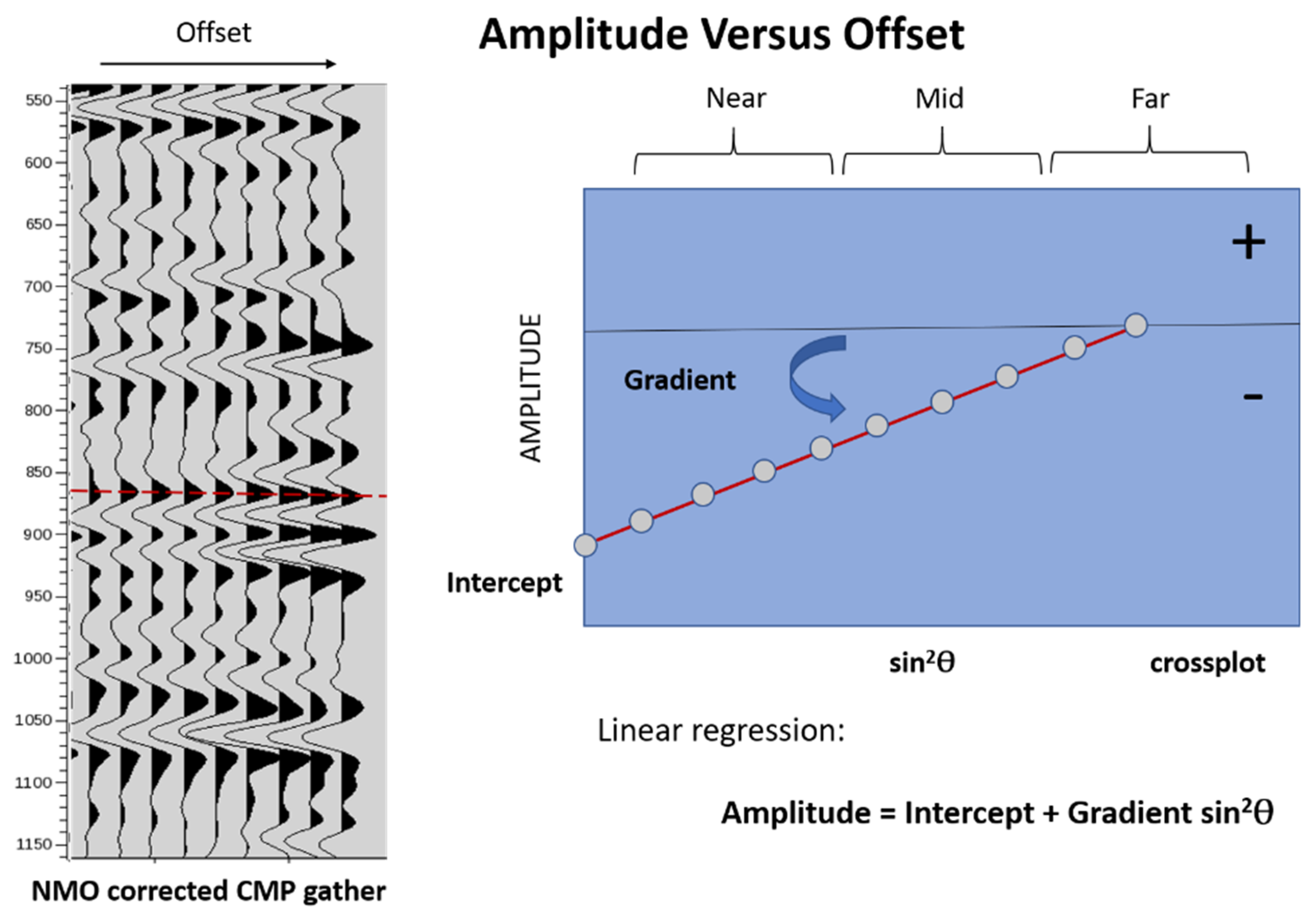
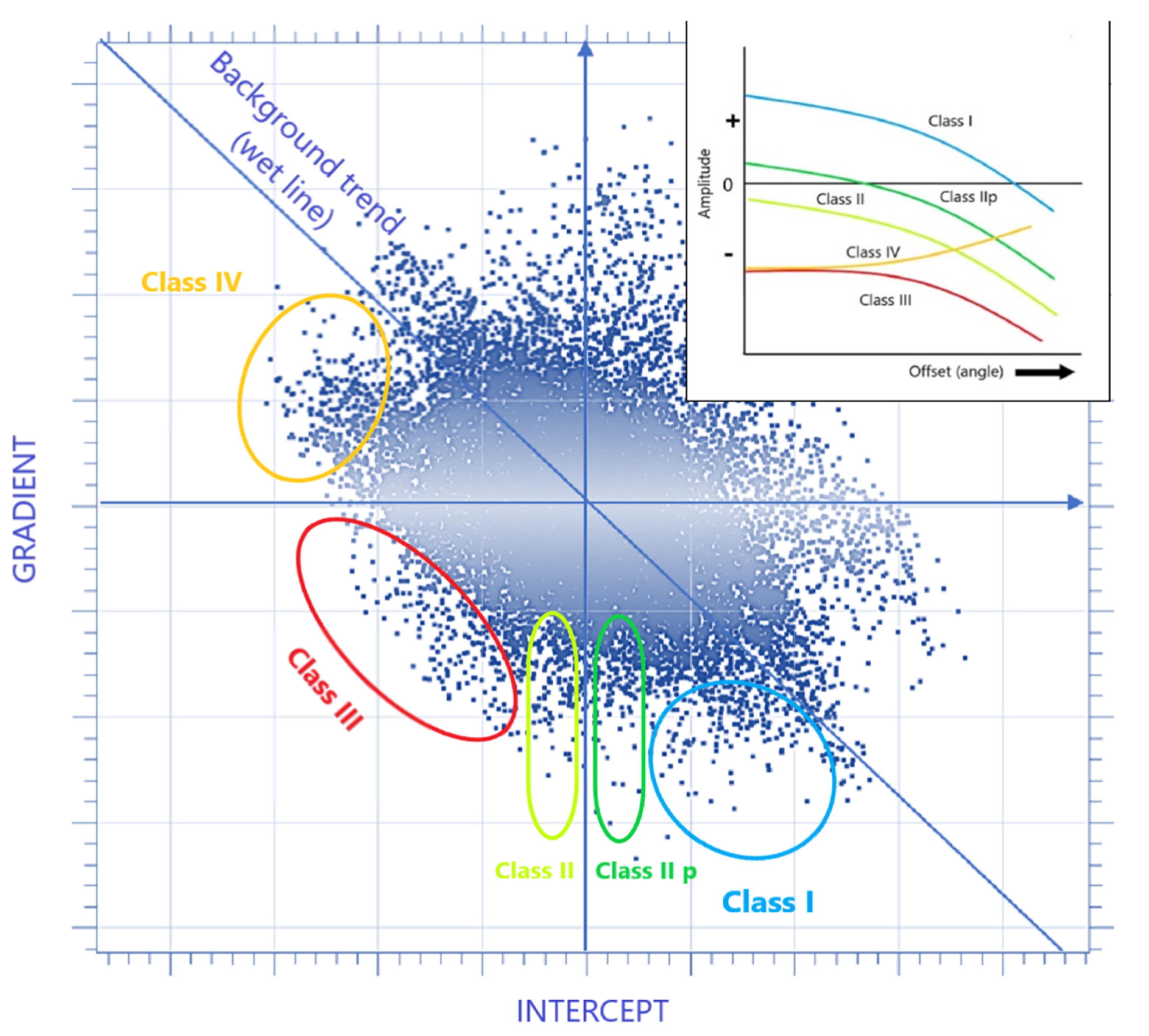
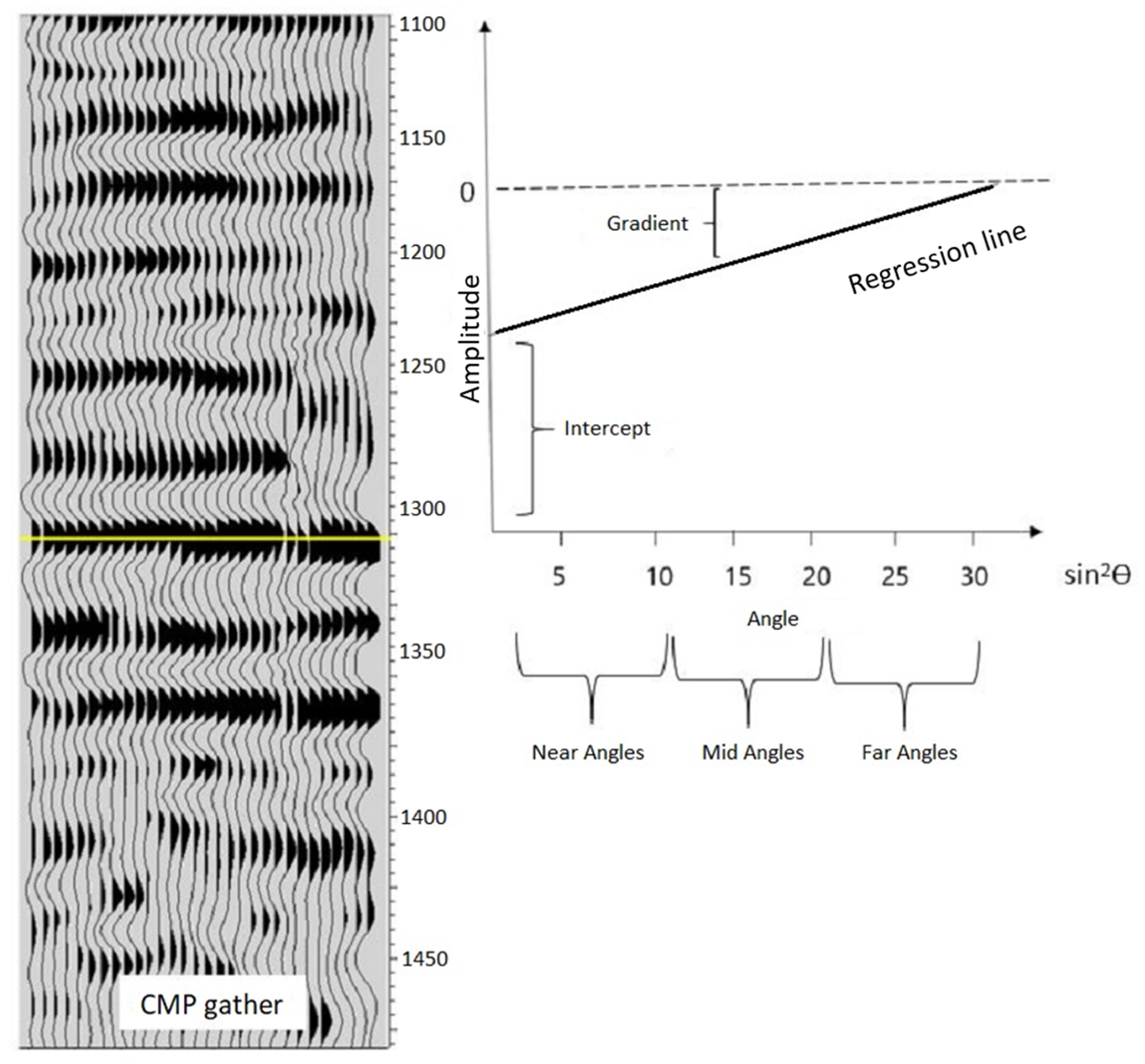
2.3. Seismic Attribute and AVO Analysis

Seismic attributes are a compendium of all the measured, computed or observed information obtained from seismic data that can greatly contribute to better interpretation of the subsurface [14].

Any value derived from seismic data can be a seismic attribute using primary differentiated attributes, instantaneous amplitude, frequency and phase and all possible combinations are derived from them. By analyzing seismic attributes, detailed reservoir characterization and quantification can be obtained. The majority of attributes are derived from post-stack data, however there are a few pre-stack attributes. The first attributes developed were related to the 1D complex seismic trace and included: envelope amplitude, instantaneous phase, instantaneous frequency, and apparent polarity. Acoustic impedance obtained from seismic inversion can also be considered an attribute and was among the first developed [15].

Commonly used attributes in the exploration and detection process of possible hydrocarbons accumulations are variance, azimuth, dip, sweetness, spectral decomposition and AVO primary and secondary attributes.

The instantaneous amplitude, also known as reflection strength, is defined as the total energy of a seismic trace. High values of amplitudes are most often related to discordances, sudden lithological changes and boundaries caused by changes in the deposition environment. Instantaneous phase is a seismic attribute that gives equal weight to both strong and weak reflexes and is a good indicator of discontinuity, slope change and layer boundaries. Instantaneous frequency shows the time change of the current phase and is used in understanding the properties of reservoirs.

Sweetness is a seismic attribute used to highlight thick, clean reservoirs, along with hydrocarbons contained within [16]. Sweetness is calculated by dividing the instantaneous amplitude (amplitude envelope) by the square root of the instantaneous frequency. This attribute detects coarse-grained intervals. These intervals are highlights on the seismic section and are called sweet spots. They indicate the possible accumulation of gas or oil.

Amplitude versus offset (AVO) is primarily the variation in seismic reflection amplitude with change in distance between shot point and the receiver [3]. Simultaneous variations in amplitude are analyzed as a function of the incidence angle, also referred to as AVA (amplitude versus angle). By using linear regression or calculating the equivalent from seismic data, it is possible to calculate the line that describes how the amplitude changes with offset or angle using the intercept and the gradient as the primary attributes. Changes in amplitude can be displayed on their crossplot as single points.

Knott and Zoeppritz developed the theoretical work necessary for AVO theory [17,18], given the P-wave and S-wave velocities along with the densities of the two-bounding media. They developed equations for plane-wave reflection amplitudes as a function of incident angle.

Different authors later gave various simpler approximations of Zoeppritz’s equations. P. Richards and C. Frasier [19] expanded the terms for the reflection and transmission coefficients for a P-wave incident upon a solid–solid interface and simplified the result by assuming only small changes in elastic properties across the interface. This approximation was popularized in 1980 by K. Aki and P. Richards [20] and has since been commonly referred to as the Aki and Richards approximation.

Ostrander [21] was the first to introduce a practical application of the AVO effect, showing that a gas sand underlying a shale exhibited amplitude variation with offset.

Shuey [22] published a closed form approximation of the Zoeppritz equations. An approximation to the Shuey equation, which itself is an approximation of the Aki–Richards equation. It is essentially the same as the Shuey equation, with the simplification that the third term is ignored (Equations (1)–(3)),

R(Ө)R (0) + Gsin² Ө

(1)

where

$$\mathrm{R}\left(0\right)=\frac{1}{2}\left(\frac{\mathsf{\Delta }\mathrm{Vp}}{\mathrm{Vp}}+\frac{\mathsf{\Delta }\mathsf{\rho }}{\mathsf{\rho }}\right)$$

(2)

and

$$\mathrm{G}=\frac{1}{2}\frac{\mathsf{\Delta }\mathrm{Vp}}{\mathrm{Vp}}-2\frac{\mathrm{Vs}2}{\mathrm{Vp}2}(\frac{\mathsf{\Delta }\mathsf{\rho }}{\mathsf{\rho }}+2\frac{\mathsf{\Delta }\mathrm{Vs}}{\mathrm{Vs}})$$

(3)

where: R is the P-wave reflection amplitude, R(0) shows the zero-offset reflectivity, θ is the average of the incidence and transmission angles, Vp is the P-wave velocity, Vs is the S-wave velocity and ρ is the density of the reflector. ∆Vp is the P-wave velocity contrast across the interface, ∆Vs is the S-wave velocity contrast across the interface and ∆ρ is the density contrast across the interface.

Equation (1) is mostly used in reservoir exploration as one of the direct hydrocarbon indicators (DHI) and is known as Shuey’s two-term AVO equation. Data from the offset domain must be transformed into an angle domain to calculate the intercept and gradient using linear regression. The condition is that the equation is linear if the intercept is a function of the incidence angle. Amplitudes picked along a moveout-corrected event on a common-midpoint (CMP) gather plotted against sin²θ can be fitted to a straight line. The slope of the line gives the AVO gradient attribute and the ordinate at zero angle gives the AVO intercept attribute. This relationship is the one expressed by AVO crossplots, which usually show intercept R(0) (the zero-offset reflectivity) plotted against gradient G.

CDP gathers are transformed from the offset domain to the angle domain and analyzed to detect changes in amplitude relative to the offset because a sudden increase in amplitude may indicate gas saturation. Polarity changes indicating a particular AVO class are also observed. Intercept I (representing the segment on the y-axis showing the amplitude) and gradient G (showing the slope of the regression line) are calculated by the linear regression method. The diagram shows the amplitude versus angle of incidence sin²θ (Figure 4).

The generated attributes by the Shuey 2-terms method, intercept and gradient, are known as the primary AVO attributes of the linear approximation. From the primary attributes, secondary AVO attributes can also be calculated. Some secondary attributes are: product of intercept and gradient (indicates in a single volume the polarity and the angle dependence of the amplitude variations) and attribute Sign(intercept) × gradient (keeps the value of gradient but the result will be directly affected according to the combined values of intercept and gradient) which were used for the calculation in this case. Primary and secondary attributes were calculated from angle stacks (near angle stack; 0–10°, mid angle stack; 10–20°, far angle stack 20–30°). Angle stacks calculated from CMP gather with carefully selected angles for near, middle and far offsets.

AVO crossplots are a simple and elegant way of representing AVO data. A central concept that emerged from this work was the “fluid line,” or background trend, a hypothetical trend based on consideration of brine filled rock properties together with simplifications of the reflectivity equations.

If the intercept is plotted on the x-axis and the gradient on the y-axis, then for consolidated sand/shale rocks the top and base reflections form a trend from the upper left to the lower right quadrant of the crossplot that passes through the origin. When it was realized that data points for equivalent hydrocarbon-filled rocks plot to the left of this line, it became clear that normalizing the data against the fluid line might provide an optimum AVO indicator [24].

The classical works dedicated to AVO cross-plotting analysis [25,26] identified four types of gas sands based on their AVO characteristics. These can be summarized as follows (Figure 5):

Class I sands are characterized by higher acoustic impedances than those of the encasing shale. They are generally found in hard rocks at depth with lower porosities. They produce positive reflection coefficients, which decrease with angle.

Class II sands have almost the same impedance as the encasing shale. Hence, they have moderate positive or negative reflection coefficients, which results in strong negative coefficient at larger angle. In some circumstances this implies phase reversal between near and far angle.

Class III sands have lower impedances than the encasing shale. They are very common in the shallow subsurface. Class III reflection coefficients increase in absolute value with increasing angle of incidence.

Class IV (added by Castagna after Rutherford–Williams) sands may have identical normal incidence reflection coefficients as per Class III, but the magnitude of Class IV sand reflection coefficients decreases in absolute value with increasing angle of incidence.

2.4. Artificial Neural Networks

Artificial neural networks (ANNs) are tolls used widely in modern scientific purposes whilst their origin can be tracked to research [30] with numerous state of the art applications in geosciences [31,32,33]. Their employment in the last several decades in the task of reservoir engineering, enhanced oil recovery and subsurface characterization in general has seen large potential [34,35,36,37]. Fundamentally, there are two different types of ANN based on their learning principles. The first incorporates supervised learning when the ANN has a set of input data with desired outcomes on which they learn and form an algorithm. The second type are self-organizing artificial neural networks (SOANNs) with unsupervised learning principles where only an input data set is given, and the task of the network is to classify the data based on their similarity. One of the applications of SOANN is a cluster analysis using Kohonen training [38] as lithology prediction from various geophysical data [39,40,41]. Earlier research in similar stratigraphic intervals and geographical extent were limited to supervised ANNs for the purpose of lithology [14,42] and hydrocarbon saturation prediction [43]. Cluster analysis using SOANN for the purpose of this research was performed using StatSoft Statistica.

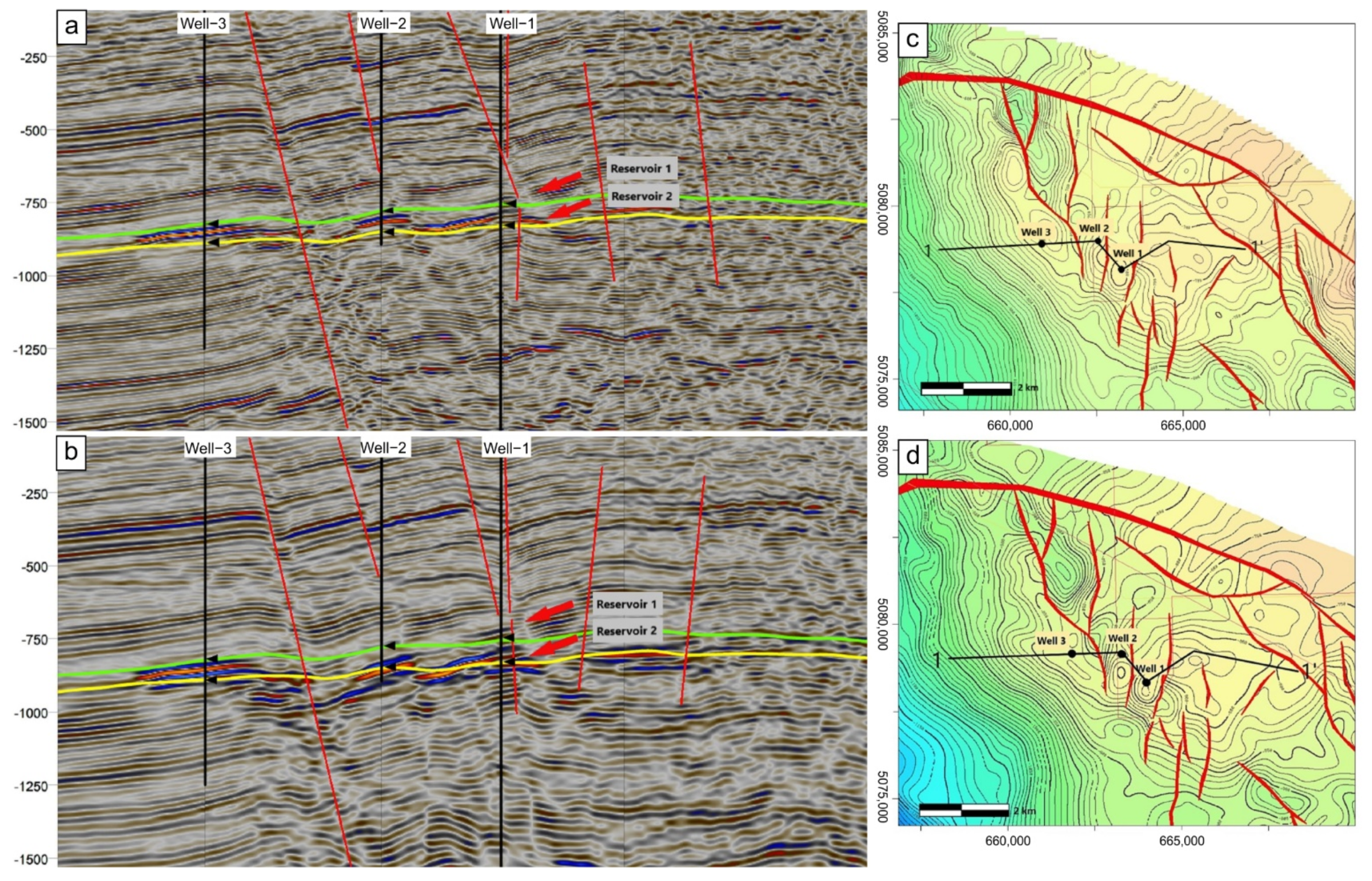
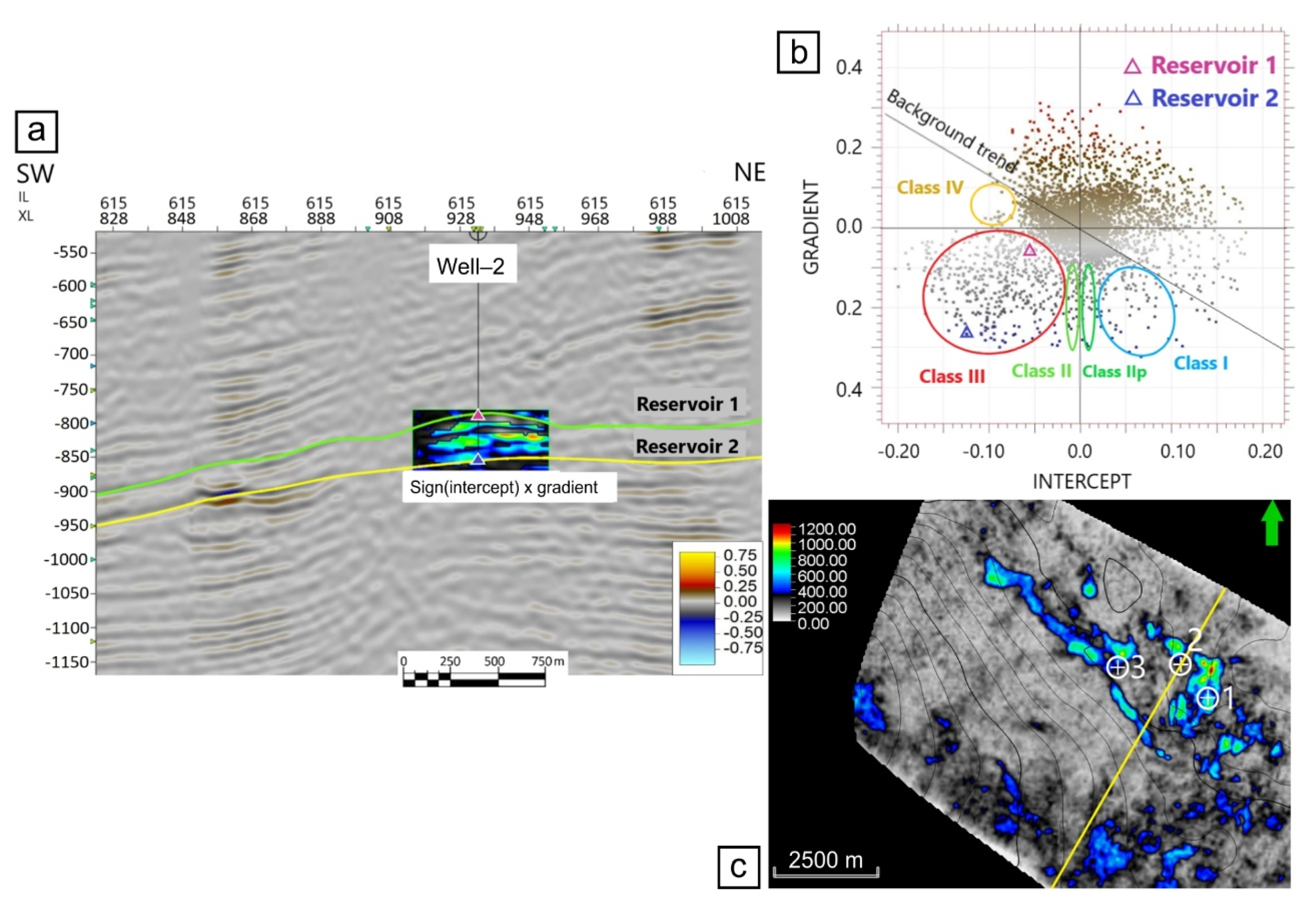
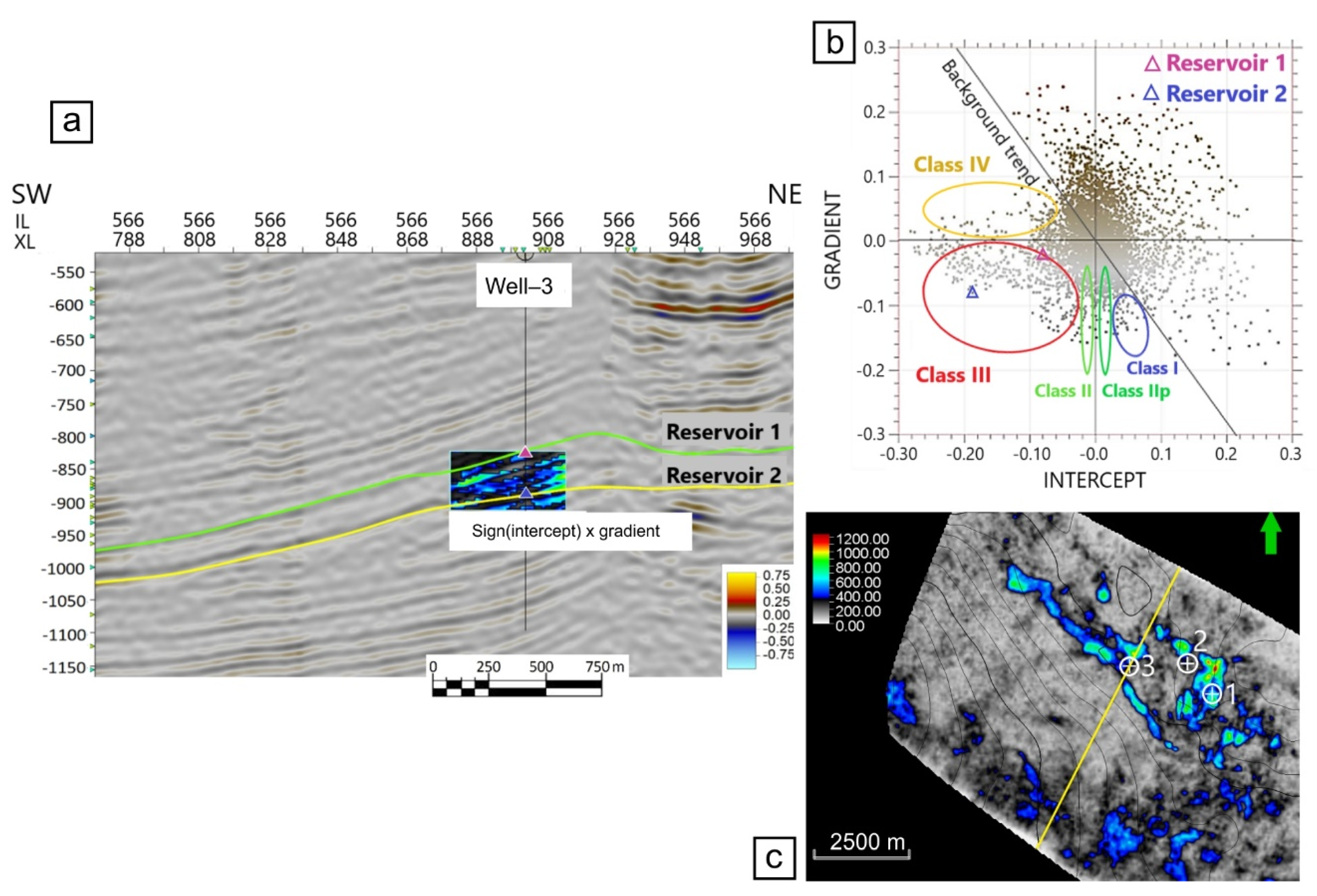
3. Results and Discussion

The sweetness seismic attribute is a very useful tool for proper description of the depositional environment, reservoir quality and lithofacies discrimination. It is very useful in fluvial systems for the identification of isolated sand bodies because they generate stronger and broader reflections than the surrounding shales. It becomes less useful in environments where sands and shales are highly interbedded or where contrasts in acoustic impedance between sands and shales are low. Sweetness improves the imaging of sand intervals or bodies and identifies oil and gas prone places called “sweet spots” [44].

On the RMS amplitude maps on the volume of sweetness attribute along the top of horizon of the Reservoir 1 (Figure 6), a small anomaly is visible in the area of the positive Well-1, while the other two negative wells are de facto in the area of lower amplitudes. The area southeast of Well-1 shows the location of highly increased amplitude which may possibly indicate gas saturation. The RMS amplitude map shown in the same way on the volume of the sweetness attribute along the top of Reservoir 2 (Figure 6) shows a positive Well-1 surrounded by a highly visible anomaly while the other two wells are in the low amplitude zone. The perspective area to the southeast is in the zone of higher amplitudes. It is possible that there is gas saturation but further consideration and other analyses are needed.

AVO analysis on the exploration area done on available pre-stack depth migration seismic volume. AVO attributes analyzed via crossplot intercept/gradient. Normally, amplitude decreases with offset. Increasing amplitude with distance from the source (offset) can be used to predict the gas saturation areas. The AVO anomaly is present at all three well locations and is also present to the south of Well-1. The anomaly can be seen in all four classes which may indicate possible gas saturation. A limitation of AVO analysis using only P-energy is its failure to yield a unique solution, so AVO results are prone to misinterpretation. One common misinterpretation is the failure to distinguish a gas-filled reservoir from a reservoir having only partial gas saturation (e.g., “fizz water “) [45]. It is nearly impossible to distinguish “fizz water sand units” from “commercial gas sand units by just using P-wave impedance or P-P reflectivity data. This is because “fizz water sand units” and “commercial gas sand units” have similar P-wave impedances (or the difference is so small that it is unresolvable seismically) [46].

The S-wave for all three wells was not recorded. In that case, sometimes, we can try using very far (beyond 30°) offset data. At far offset, seismic reflections are heavily influenced by not only the P-wave impedances, but also the S-wave impedances, the P-S impedance ratio, and density contrasts. As a result, very far offset seismic data could contain information on the amount of gas saturation, giving potential to distinguish “fizz water sand units” from “commercial gas sand units”. This of course depends on the quality of very far offset data and many other challenging factors [46].

On the seismic profile of the volume of the intercept (primary AVO attribute calculated from Angle stacks) through the Well-1 within the volume of interest (220 ms -XL888-XL948) the volume Sign(intercept) × gradient is overlapped where between the top of horizons of Reservoir 1 and Reservoir 2, inside the window clearly visible increase in amplitude in green, yellow and red, which indicates the possible presence of gas (Figure 7a). The Intercept/gradient crossplot shows a deviation from the background trend or AVO anomalies in all 4 classes (Figure 7b) On Well-1 along the top of horizons of Reservoirs 1 and 2. Furthermore, extracted AVO anomalies at one point shown in crossplot intercept/gradient as a pink triangle for Reservoir 1 which shows that the point falls within the third quadrant and shows AVO class III. The blue triangle shows Reservoir 2 also within the AVO class III.

The Figure 7c shows a map of RMS amplitudes on the volume Sign(intercept) × gradient between the top of horizons of reservoirs 1 and 2 with a calculated window of 10 ms above Reservoir 1 and below Reservoir 2. Furthermore, increasing amplitude of Well-1 is visible, confirming the presence of gas.

The same procedure was also performed for Well-2 and Well-3, the drilling of which did not confirm the presence of gas as in positive Well-1, as well as for potential area southeast of Well-1.

A window with a volume of interest of 180 ms (XL 916–950) was taken for Well-2 (Figure 8a). For Well-3 (Figure 9a), a window of 150 ms (XL 880–915), and for the anomaly area southeast of Well-1 (Figure 10a), a window with a size of 200 ms (XL 848–910). Within the volume of interest, an increase in amplitudes in green, yellow and red is shown.

Furthermore, the other two wells and the anomaly area on the southeast show the AVO anomaly at one point, the pink triangle for Reservoir 1 and the blue for Reservoir 2 located overall within the third quadrant, AVO class III (Figure 8b, Figure 9b and Figure 10b).

RMS amplitude maps at the Sign(intercept) × gradient volume between the tops of the horizons of both reservoirs it is evident that an anomaly exists, but around the two negative wells, not at their locations (Figure 8c and Figure 9c). To the southeast, in the perspective area, the anomaly is clearly visible (Figure 10c).

The AVO anomaly is also visible on two negative wells 2 and 3 in all 4 classes, but where class III which represents the classic bright spot is very visible. A limitation of AVO analysis using only P-energy is its failure to yield a unique solution, so AVO results are prone to misinterpretation. One common misinterpretation is the failure to distinguish a gas-filled reservoir from a reservoir having only partial gas saturation (“fizz water”). The S-wave was not recorded. Very small amounts of gas at two wells have the same Vp/Vs ratio as with 90% gas saturation, thus the AVO anomaly does not differ between 5 and 90% of saturation gas.

When there are no records of the S-wave, sometimes very far offset seismic data could give the potential to distinguish “fizz”-gas from “commercial gas sand units”. Far angle stacks are calculated with angles of 20–30 degrees. However, we also calculated a version with slightly larger angles of 24–36 degrees. The figure shows the extracted RMS amplitude on the far angle stack (with larger angles) volume along the top of Reservoir 1 (Figure 11a), and the figure shows the top of Reservoir 2 (Figure 11b) in the same way. Amplitude increases are present on both reservoirs on Well-1 as well as southeast in the potential area. Negative wells are located near anomalies. We cannot determine with accuracy that these anomalies do not show only very small amounts of gas and more detailed analyses should be made.

SOANN analysis was performed using TIBCO STATISTICA software on the top of Reservoir 1 horizon through the available 3D volume in order to recognize the patterns that could implicate the variation of lithology, gas accumulation anomalies or structural elements. Almost 170,000 data points were extracted from the surface which relates to Reservoir 1 top with associate seismic attribute values of envelope, instantaneous frequency, sweetness, RMS amplitudes, chaos and cosine of phase. Two outcomes with topological cluster maps of 2 × 2 and 3 × 3 dimensions were made to visualize the features on top of the Reservoir 1 horizon. Limit for the learning process was set for 1000 iterations using Kohonen training. Learning process results present relatively small amounts of errors in the classification of seismic data within the categories (

Table 1. Self-organizing neural network learning process result.

Neural Network Architecture	Training Error (%)	Test Error (%)
2 × 2 SOANN	5.2	8.4
3 × 3 SOANN	3.4	4.8

).

SOANN with 2 × 2 neural network architecture/topological map resulted in data being divided into 4 classes and 3 × 3 architecture. Data points with associated classes were imported into petrel where there were upscaled within a simple model representing the top of the Reservoir 1 horizon. All three wells fell in the same class category which pointed out that this kind of approach can hardly distinguish gas presence within the area of the research (Figure 12). However, structural features such as faults (linear features of category distribution) and sedimentological features can be observed which presents a possible path for further research for SAONN approaches within 3D seismic volumes.

4. Conclusions

AVO analysis on the exploration area done on available pre-stack depth migration seismic volume. AVO attributes analyzed via crossplot intercept/gradient. Normally, amplitude decreases with offset. Increasing amplitude with distance from the source (offset) can be used to predict the gas saturation areas. The AVO anomaly is present at all three well locations and is also present southeast of Well-1. The data were extracted at one point for each reservoir and each well, and are located within the third quadrant on the crossplot intercept/gradient and show AVO class III.

AVO class III shows an increase in amplitude with distance and shows a classic bright spot. This also means that there is a large difference in acoustic impedances between the reflectors. The reason may be sudden lithological changes as well as very small amounts of gas.

Only a small percent of the gas will cause a significant drop in the effective fluid modulus, and consequently a significant drop in the bulk modulus in the rock. Therefore, P-wave seismic can usually only determine the presence of gas, but not saturation.

The S-wave was not recorded for any wells. Therefore, we cannot confirm the amount of saturation with certainty. However, other methods such as the analysis of the seismic attribute sweetness and the extracted RMS amplitude on the far angle stack can help us. Two negative wells are located outside or on the edge of anomalies. Further studies will confirm whether commercial gas saturation exists within the larger anomaly.

Distinguishing “fizz water” from “commercial gas” saturations with surface seismic and borehole data remains a challenging problem. The solution and help can be in obtaining and using quality S-wave data, scaling and attenuation in data processing and analysis of other seismic attributes.

Although SOANN did not yield the desired result of distinguishing the locations of possible gas accumulations, the structural and sedimentological features which can be observed on top of Reservoir 1 horizon present a potential for future SOANN application.

References

1. Velić, J.; Krasić, D.; Kovačević, I. Exploitation, reserves and transport of natural gas in the Republic of Croatia. Teh. Vjesn. Gaz. 2012, 13, 633–641. [Google Scholar]
2. Farkaš Višontai, L.; Brusić, N.; Ilišević, I.; Novaković, N.; Jakovac, B.; Perić, M.; Križan, J. 20 years of gas production in the Adriatic [20 godina proizvodnje plina na Jadranu]. Naft. Plin. 2019, 39, 39–52. [Google Scholar]
3. Hussein, M.; El-Ata, A.A.; El-Behiry, M. AVO analysis aids in differentiation between false and true amplitude responses: A case study of El Mansoura field, onshore Nile Delta, Egypt. J. Pet. Explor. Prod. Technol. 2020, 10, 969–989. [Google Scholar] [CrossRef] [Green Version]
4. Malvić, T.; Cvetković, M. Lithostratigraphic units in the Drava Depression (Croatian and Hungarian parts)—A correlation. Nafta 2013, 63, 27–33. [Google Scholar]
5. Cvetković, M.; Matoš, B.; Rukavina, D.; Kolenković Močilac, I.; Saftić, B.; Baketarić, T.; Baketarić, M.; Vuić, I.; Stopar, A.; Jarić, A.; et al. Geoenergy potential of the Croatian part of Pannonian Basin: Insights from the reconstruction of the pre-Neogene basement unconformity. J. Maps 2019, 15, 651–661. [Google Scholar] [CrossRef] [Green Version]
6. Dolton, G.L. Pannonian Basin Province, Central Europe (Province 4808)—Petroleum Geology, Total Petroleum Systems, and Petroleum Resource Assessment; USGS: Reston, Virginia, 2006. [Google Scholar]
7. Schmid, S.M.; Bernoulli, D.; Fügenschuh, B.; Matenco, L.; Schefer, S.; Schuster, R.; Tischler, M.; Ustaszewski, K. The Alpine-Carpathian-Dinaridic orogenic system: Correlation and evolution of tectonic units. Swiss J. Geosci. 2008, 101, 139–183. [Google Scholar] [CrossRef] [Green Version]
8. Pavelić, D.; Kovačić, M. Sedimentology and stratigraphy of the Neogene rift-type North Croatian Basin (Pannonian Basin System, Croatia): A review. Mar. Pet. Geol. 2018, 91, 455–469. [Google Scholar] [CrossRef]
9. Royden, L. Late Cenozoic tectonics of the Pannonian Basin system. In The Pannonian Basin: A Study in Basin Evolution. AAPG Memoir 45; Royden, L.H., Horvath, F., Eds.; AAPG: Tulsa, OK, USA, 1988. [Google Scholar]
10. Lučić, D.; Saftić, B.; Krizmanić, K.; Prelogović, E.; Britvić, V.; Mesić, I.; Tadej, J. The Neogene evolution and hydrocarbon potential of the Pannonian Basin in Croatia. Mar. Pet. Geol. 2001, 18, 133–147. [Google Scholar] [CrossRef]
11. Malvić, T. Geological maps of Neogene sediments in the Bjelovar Subdepression (Northern Croatia). J. Maps 2011, 7, 304–317. [Google Scholar] [CrossRef]
12. Ćorić, S.; Pavelić, D.; Rögl, F.; Mandić, O.; Vrabac, S.; Avanić, R.; Jerković, L.; Vranjković, A. Revised Middle Miocene datum for initial marine flooding of North Croatian Basins (Pannonian Basin System, Central Paratethys)The Pannonian Basin System (PBS) originated during the Early Miocene as a result of extensional processes between the Alpine-Carp. Geol. Croat. 2009, 62, 31–43. [Google Scholar] [CrossRef]
13. Šimon, J. O nekim rezultatima regionalne korelacije litostratigrafskih jedinica u jugozapadnom području Panonskog bazena. Nafta 1973, 24, 623–630. [Google Scholar]
14. Brcković, A.; Kovačević, M.; Cvetković, M.; Močilac, I.K.; Rukavina, D.; Saftić, B. Application of artificial neural networks for lithofacies determination based on limited well data. Cent. Eur. Geol. 2017, 60, 299–315. [Google Scholar] [CrossRef]
15. Sheriff, R.E. Vertical and Lateral Seismic Resolution and Attenuation: Part 7. Geophysical Methods. In ME 10: Development Geology Reference Manual; Morton-Thompson, D., Woods, A.M., Eds.; AAPG: Tulsa, OK, USA, 1992; pp. 388–389. [Google Scholar]
16. SEG Sweetness. Available online: https://wiki.seg.org/wiki/Sweetness (accessed on 25 February 2021).
17. Knott, C.G., III. Reflexion and refraction of elastic waves, with seismological applications. London Edinburgh Dublin Philos. Mag. J. Sci. 1899, 48, 64–97. [Google Scholar] [CrossRef] [Green Version]
18. Zoeppritz, K. On the Reflection and Transmission of Seismic Waves at Surfaces of Discontinuity. In Classics of Elastic Wave Theory; Society of Exploration Geophysicists: Tulsa, OK, USA, 2007; pp. 363–376. [Google Scholar]
19. Richards, P.G.; Frasier, C.W. Scattering of elastic waves from depth-dependent inhomogeneities. Geophysics 1976, 41, 441–458. [Google Scholar] [CrossRef]
20. Aki, K.; Richards, P.G. Quantitative Seismology: Theory and Methods; Freeman and Co.: San Francisco, CA, USA, 1980; Volumes I. & II. [Google Scholar]
21. Ostrander, W.J. Plane-Wave Reflection Coefficients for Gas Sands at Nonnormal Angles of Incidence. Explor. Geophys. 1984, 49, 1580–1813. [Google Scholar] [CrossRef]
22. Shuey, R.T. A simplification of the Zoeppritz equations. Geophysics 1985, 50, 609–614. [Google Scholar] [CrossRef]
23. Veeken, P.C.H.; Rauch-Davies, M. AVO attribute analysis and seismic reservoir characterization. First Break 2006, 24, 41–52. [Google Scholar] [CrossRef]
24. Simm, R.; White, R.; Uden, R. The anatomy of AVO crossplots. Lead. Edge 2000, 19, 150–155. [Google Scholar] [CrossRef]
25. Rutherford, S.R.; Williams, R.H. Amplitude-versus-offset variations in gas sands. Geophysics 1989, 54, 680–688. [Google Scholar] [CrossRef]
26. Castagna, J.P.; Swan, H.W. Principles of AVO crossplotting. Lead. Edge 1997, 16, 337–344. [Google Scholar] [CrossRef]
27. Castagna, J.P.; Smith, S.W. Comparison of AVO indicators: A modeling study. Geophysics 1994, 59, 1849–1855. [Google Scholar] [CrossRef]
28. Ross, C.P.; Kinman, D.L. Nonbright-spot AVO: Two examples. Geophysics 1995, 60, 1398–1408. [Google Scholar] [CrossRef]
29. Castagna, J.P.; Swan, H.W.; Foster, D.J. Framework for AVO gradient and intercept interpretation. Geophysics 1998, 63, 948–956. [Google Scholar] [CrossRef]
30. Rosenblatt, F. The perceptron: A probabilistic model for information storage and organization in the brain. Psychol. Rev. 1958, 65, 386–408. [Google Scholar] [CrossRef] [PubMed] [Green Version]
31. Qu, D.; Frykman, P.; Stemmerik, L.; Mosegaard, K.; Nielsen, L. Upscaling of outcrop information for improved reservoir modelling—Exemplified by a case study on chalk. Pet. Geosci. 2021, petgeo2020-126. [Google Scholar] [CrossRef]
32. Iturrarán-Viveros, U.; Muñoz-García, A.M.; Parra, J.O.; Tago, J. Validated artificial neural networks in determining petrophysical properties: A case study from Colombia. Interpretation 2018, 6, T1067–T1080. [Google Scholar] [CrossRef]
33. Okon, A.N.; Adewole, S.E.; Uguma, E.M. Artificial neural network model for reservoir petrophysical properties: Porosity, permeability and water saturation prediction. Model. Earth Syst. Environ. 2020. [Google Scholar] [CrossRef]
34. Thanh, H.V.; Sugai, Y.; Nguele, R.; Sasaki, K. Integrated workflow in 3D geological model construction for evaluation of CO2 storage capacity of a fractured basement reservoir in Cuu Long Basin, Vietnam. Int. J. Greenh. Gas. Control. 2019, 90, 102826. [Google Scholar] [CrossRef]
35. Thanh, H.V.; Sugai, Y. Integrated modelling framework for enhancement history matching in fluvial channel sandstone reservoirs. Upstream Oil Gas. Technol. 2021, 6, 100027. [Google Scholar] [CrossRef]
36. Thanh, H.V.; Sugai, Y.; Sasaki, K. Application of artificial neural network for predicting the performance of CO2 enhanced oil recovery and storage in residual oil zones. Sci. Rep. 2020, 10, 18204. [Google Scholar] [CrossRef]
37. Thanh, H.V.; Sugai, Y.; Sasaki, K. Impact of a new geological modelling method on the enhancement of the CO 2 storage assessment of E sequence of Nam Vang field, offshore Vietnam. Energy Sources Part. A Recover. Util. Environ. Eff. 2020, 42, 1499–1512. [Google Scholar] [CrossRef]
38. Kohonen, T. Self-organized formation of topologically correct feature maps. Biol. Cybern. 1982, 43, 59–69. [Google Scholar] [CrossRef]
39. Asfahani, J.; Ahmad, Z.; Ghani, B.A. Self organizing map neural networks approach for lithologic interpretation of nuclear and electrical well logs in basaltic environment, Southern Syria. Appl. Radiat. Isot. 2018, 137, 50–55. [Google Scholar] [CrossRef] [PubMed]
40. Dixit, N.; McColgan, P.; Kusler, K. Machine Learning-Based Probabilistic Lithofacies Prediction from Conventional Well Logs: A Case from the Umiat Oil Field of Alaska. Energies 2020, 13, 4862. [Google Scholar] [CrossRef]
41. Bauer, K.; Muñoz, G.; Moeck, I. Pattern recognition and lithological interpretation of collocated seismic and magnetotelluric models using self-organizing maps. Geophys. J. Int. 2012, 189, 984–998. [Google Scholar] [CrossRef] [Green Version]
42. Kamenski, A.; Cvetković, M.; Kolenković Močilac, I.; Saftić, B. Lithology prediction in the subsurface by artificial neural networks on well and 3D seismic data in clastic sediments: A stochastic approach to a deterministic method. GEM Int. J. Geomath. 2020, 11, 8. [Google Scholar] [CrossRef] [Green Version]
43. Cvetkovic, M.; Velic, J.; Malvic, T. Application of neural networks in petroleum reservoir lithology and saturation prediction. Geol. Croat. 2009, 62, 115–121. [Google Scholar] [CrossRef]
44. Novak Zelenika, K.; Novak Mavar, K.; Brnada, S. Comparison of the Sweetness Seismic Attribute and Porosity–Thickness Maps, Sava Depression, Croatia. Geosciences 2018, 8, 426. [Google Scholar] [CrossRef] [Green Version]
45. Singh, D. AVO Techniques: Advantages, Limitations and Future Prospects. In Proceedings of the 8th Biennial International Conference & Exposition on Petroleum Geophysics, Hyderabad, India, 1–3 February 2010; pp. 1–3. [Google Scholar]
46. Chopra, S. Expert Answers | October 2004 | CSEG RECORDER. Available online: https://csegrecorder.com/columns/view/expert-answers-200410 (accessed on 23 May 2021).
Figure 1. Overview of the main tectonic and geographical units of the Pannonian Basin with outline of the Bjelovar Subdepression location (modified after [5,6,7] with references).
Energies 14 04161 g001
Figure 2. Schematic lithostratigraphic column of the western part of the Drava Depression, valid for the Bjelovar Subdepression, with main tectonic events and well log markers. Modified from [4,13].
Energies 14 04161 g002
Figure 3. Reprocessed and reinterpreted data (pre-stack time migration (a), pre-stack depth migration (b)) with structural maps on top of Reservoir 1 (c) and Reservoir 2 (d).
Energies 14 04161 g003
Figure 4. Amplitude versus offset (AVO) attributes computed in an amplitude-versus-sin2θ crossplot. The regression line gives the intercept I (cutoff on the Y-axis) and the gradient G (the slope of the line) that defines the rate of change in amplitude with offset (from [23]).
Energies 14 04161 g004
Figure 5. AVO cross-plotting, AVO classes after [25], originally defined for gas sands (classes I, II and III), along with the added classes IV [27] and IIp [28]. Figure modified from [25,29].
Energies 14 04161 g005
Figure 6. Extracted RMS amplitude along the horizons of the top of Reservoir 1 on the volume of sweetness attribute and Reservoir 2.
Energies 14 04161 g006
Figure 7. Seismic profile on the volume of the primary AVO attribute intercept through Well-1 with overlapping secondary AVO attribute Sign(intercept) × gradient inside the window around reservoirs 1 and 2 (a). AVO (intercept/gradient) crossplot with anomalies in all 4 classes (b) and extracted RMS amplitude between the horizons of the tops of Reservoir 1 and Reservoir 2 on the volume of the secondary AVO attribute Sign(intercept) × gradient with the displayed profile through Well-1 (c).
Energies 14 04161 g007
Figure 8. Seismic profile on the volume of the primary AVO attribute intercept through Well-2 with overlapping secondary AVO attribute Sign(intercept) × gradient inside the window around reservoirs 1 and 2 (a). AVO (intercept/gradient) crossplot with anomalies in all 4 classes (b) and extracted RMS amplitude between the horizons of the tops of Reservoir 1 and Reservoir 2 on the volume of the secondary AVO attribute Sign(intercept) × gradient with the displayed profile through Well-1 (c).
Energies 14 04161 g008
Figure 9. Seismic profile on the volume of the primary AVO attribute—intercept through Well-3 with overlapping secondary AVO attribute Sign(intercept) × gradient inside the window around reservoirs 1 and 2 (a). AVO (intercept/gradient) crossplot with anomalies in all 4 classes (b) and extracted RMS amplitude between the horizons of the tops of Reservoir 1 and Reservoir 2 on the volume of the secondary AVO attribute Sign(intercept) × gradient with the displayed profile through Well-1 (c).
Energies 14 04161 g009
Figure 10. Seismic profile on the volume of the primary AVO attribute intercept through the area southeast of Well-1 with overlapping secondary AVO attribute Sign(intercept) × gradient inside the window around reservoirs 1 and 2 (a). AVO (intercept/gradient) crossplot with anomalies in all 4 classes (b) and extracted RMS amplitude between the horizons of the tops of Reservoir 1 and Reservoir 2 on the volume of the secondary AVO attribute Sign(intercept) × gradient with the displayed profile through the Well-1 (c).
Energies 14 04161 g010
Figure 11. Extracted RMS amplitude along the top horizon of Reservoir 1 on the volume of the far angle stack with the wells shown and the circled area southeast of Well-1 (a) and Reservoir 2 (b).
Energies 14 04161 g011
Figure 12. SOANN maps of 2 × 2 topological distribution (left) and 3 × 3 topological distribution (right) on top of Reservoir 1 horizon.
Energies 14 04161 g012