1. Introduction
Current strategies to address climate change share a fundamental assumption: Containment of greenhouse gases hinges essentially on the success of behavioral changes in energy use and investment decisions [
1,
2,
3]. The low uptake of energy-efficient appliances can be, at least partially, explained by informational failures (such as imperfect and asymmetric information and myopia) and behavioral biases related, for instance, to social norms, decision-making heuristics, and inattention, e.g., [
4,
5,
6,
7,
8,
9]. Thus, it is expected that more informed, forward-looking electricity consumers would contribute to energy reduction worldwide, e.g., [
10,
11,
12,
13,
14]. The confinement measures born out of the recent pandemic have eased energy use [
15] and brought the need for restructuring the energy sector to the fore. At the same time, the measures vividly showed what can be achieved when individuals are persuaded to follow new behavioral norms [
16].
Several studies have used multiple regression models to identify patterns between market and non-market barriers and energy-efficiency investment decisions, e.g., [
4,
5,
8,
9,
12,
17,
18,
19,
20]. Nevertheless, whether these patterns are repeatable or not is not clear, because the efforts to determine the transferability or generalizability of these models are practically nonexistent. The issue of transferability is of great interest in ecological models (e.g., [
21,
22,
23]), models of air pollutants (e.g., [
24,
25,
26]), travel forecasting models (e.g., [
27,
28,
29]), and especially in non-market valuation (an approach known as “benefit function transfer,” e.g., [
30,
31,
32,
33,
34]). Concerning energy studies, the aspect of transferability has been tested in predictive models of energy customer data analytics [
35], building energy consumption data models [
36], and residential energy demand and city-scale electricity usage models [
37,
38]. In addition, Warren [
39] developed a multicriteria decision-making framework to identify whether demand-side management (DSM) policies are transferable and Bößner et al. [
40] investigated the transfer of renewable energy support policies between countries.
Bearing in mind the above-mentioned remarks, the objective of the present paper is to contribute to a behaviorally informed energy-saving strategy by filling the existing gap in the literature regarding the transferability potential of energy consumer decision-making models. As a first step, datasets were collected within the CONSEED project (
https://www.conseedproject.eu, accessed on 30 March 2021) in a number of discrete choice experiments, along with surveys and field trials. The target was different consumer groups, spatial locations, and product categories, e.g., [
12,
20,
41,
42,
43]. The data were examined and cleaned to be made suitable to pool for econometric analysis. This resulted in two homogenized datasets, as detailed in
Section 3. The two datasets were used to validate the theoretical and econometric models developed prior to the survey (for details see [
44]) Specifically, the pooled models aim to determine the relative importance of (a) market and non-market biases (e.g., mistrust of energy labels, “warm glow” motives associated with the perceived negative environmental and societal consequences of energy consumption, etc.) and (b) socio-demographic characteristics that account for agent heterogeneity in energy investment decisions. These two datasets are used to evaluate the “transferability” of the pooled models between countries and technologies, following the validation methodology discussed in
Section 2.2, an underappreciated aspect of statistical validation [
22]. Hence, the findings presented here are related to the following two hypotheses:
Proposition 1. The pooled model is valid and, therefore, provides a reliable view of the market and non-market barriers affecting consumer energy efficiency decisions.
Proposition 2. The pooled model is “transferable” between countries and technologies; that is, the identified relationships between consumer energy-investment decisions, socioeconomic factors, and market and non-market barriers are general and not idiosyncratic to a limited set of conditions.
The first proposition examines the validity of the model in terms of goodness of fit and discrimination using appropriate criteria (i.e., Pearson’s χ
2 goodness-of-fit statistic and C-statistic). The null hypothesis is that the pooled models are valid. The second proposition tests the transferability potential of the validated models between different countries, technologies, sectors, etc. The evaluation is performed using Pearson’s χ
2 goodness-of-fit and C-statistic indicators, as well as the Wald test regarding the equality of the coefficients across the models. Previous research has shown that energy efficiency-related attitudes and behavior are affected by sociodemographic characteristics [
5,
45], attitudinal characteristics [
45], and market and non-market failures (e.g., asymmetric/imperfect information, misplaced motivations, biased perceptions on the product energy consumption, etc.) [
13,
45,
46,
47,
48,
49,
50,
51]. The above-mentioned factors differ across countries, consumer goods, etc., and thus, in this case, the null hypothesis is that the models are not “transferable” in principle.
The paper is structured as follows:
Section 2 provides the methodological overview.
Section 3 presents and discusses the main results drawn from the analysis. We conclude in
Section 4 with thoughts on the potential of our model(s) to feed into cross-national European energy policy design.
2. Materials and Methods
2.1. Sample Pooling
The CONSEED partners initially set out to design surveys, discrete choice experiments, and field trials in a harmonized way to facilitate subsequent data pooling. However, the considerable heterogeneity in field trials and discrete choice experiments led to inconsistency in variables and contexts that prevented the pooling of these datasets. For example, although the results of the property and appliance field trials are comparable in terms of their treatment effects, it is not feasible or desirable to combine these two datasets consistently for ex-post analysis and verification purposes due to the very different characteristics of each dataset. Furthermore, although each discrete choice experiment included EE as an attribute, all remaining attributes differed by the technology explored, as did the experimental designs and treatment methods. Given the heterogeneity of the field trials and discrete choice experiments, pooling would not produce a workable dataset.
Of the available data types, only the consumer surveys addressed to households and firms (including farmers) are suitable for pooling and analysis. Despite considerable differences in locations (Greece, Ireland, Spain, Norway, and Slovenia), technologies (property, appliances, transport, and machinery), and sectors (households, services, agriculture, and industry), CONSEED designed a “core” set of survey questions that were applied in all surveys (see, for example,
Table S1: Common survey questions). Often, this required minor adjustments depending on the sample and context. For example, when asked about the importance of technology attributes, the set of six attributes always included energy/fuel efficiency/consumption and price, but partners had discretion in choosing four additional sample-specific attributes. In addition to this, partners had discretion in asking supplementary non-core questions in their surveys. The resulting “pooled” dataset incorporates all core survey questions only, covering households and firms.
The “households” pooled sample included 3016 observations from Norway (1093 or 36.2%), Ireland (501 or 16.6%), Spain (500 or 16.6%), Greece (496 or 16.4%), and Slovenia (426 or 14.1%). Further, 1093 observations (36.2%) concerned transportation goods, i.e., cars; 996 observations (33%) concerned household appliances, i.e., refrigerators (496 observations) and washing machines (500 observations); and 927 (30.7%) observations concerned properties. As far as the “firms” pooled sample is concerned, it included 794 observations in total. More specifically, 492 observations (62%) derived from Ireland, 200 observations (25.2%) from Spain, and 102 observations (12.8%) from Greece. As regards the technological subsamples, 302 observations (38%) involved heating and cooling appliances in the services sector, 316 observations (39.8%) concerned machinery in the agricultural sector, and 176 observations (22.2%) concerned heating controls in the properties sector.
2.2. Model Validation
Model validation is a statistical concept that hints at the model’s degree of generalizability and implies that the model chosen for measuring the theoretical concepts and relationships accurately represents the real-world phenomena [
52]. Specifically, the focus of this paper is on assessing the performance of the model on predicting the probability of the positive event for out-of-the-sample subjects [
53,
54,
55].
There are two main statistical approaches to model validation, namely, external validation (the model is tested on a new sample) and internal validation (the model is tested on a subsample of the original sample). Although external validation appears to be a rigorous validation approach, it has certain disadvantages. For instance, the collection of a new sample that will only be used in the validation of the model can be rather costly. Further, even if monetary resources are available, the new sample must be sufficiently representative of the original sample, otherwise the validation process can provide misleading results, either pessimistic or optimistic. For these reasons and due to budget constraints, the internal validation approach was adopted in this case.
The most accredited internal validation methods are data-splitting, repeated data-splitting, jackknife, and bootstrapping [
55]. In all these methods, a subsample of observations is excluded from the analysis, a model based on the remaining subjects is developed, and then it is tested on the originally excluded subjects. In this study, the repeated data splitting approach was chosen, for reasons detailed in [
55], and hence, the available data were split into two portions. The first portion was used to fit the model (i.e., fitting sample) and the second was used to assess its performance (i.e., validation sample). Usually, the portion of observations reserved for validation is always less than ½ and in the range of ¼ to ⅓ [
56], and a priori the performance of the validation model is inferior to that of the fitting sample [
55]. Fitting and validation samples in our cases were defined from original and pooled datasets.
The model validation process of the pooled samples involves the following steps described in [
55], after modifications:
Step 1: Data splitting. The pooled sample is randomly split into the fitting (70%) and validation samples (30%, to have an adequate number of observations).
Step 2: Model fitting. The model’s coefficients, its overall significance, and the partial significance of each variable are estimated on the fitting sample.
Step 3: Event probability estimation. The coefficients from Step 2 are used to estimate the probability of a positive outcome for each of the subjects in the fitting and the validation samples.
Step 4: Computation of performance measures. The fitting and validation samples are tested against the following statistics:
- -
C-statistic (a measure of predictive power);
- -
Pearson’s χ2 goodness-of-fit statistic.
The C-statistic is a measure of goodness of fit for binary outcome regression models and it is equal to the area under the receiver operating characteristic (ROC) curve and ranges from 0.5 to 1. As a general rule [
53],
if C ≥ 0.9, the model is considered to have outstanding discrimination;
if 0.8 ≤ C < 0.9, the model is considered to have excellent discrimination;
if 0.7 ≤ C < 0.8, the model is considered to have acceptable discrimination;
if C = 0.5, the model has no discrimination;
if C < 0.5, the model has negative discrimination, i.e., it is worse than random.
Pearson’s χ
2 goodness-of-fit statistic, as a measure of calibration, examines the null hypothesis that the logistic regression model used is the correct model [
57].
Step 5: Iterations. The above-described procedure is repeated 100 times. Each iteration is based on a different split of the original data and results in different model coefficients, significance levels, and performance values.
Step 6: Results. After the 100 repetitions, the distribution of each of the performance measures is provided for the fitting and validation samples. As mentioned, in general, a reduction in the magnitude of discrimination and calibration performance is expected, but if the drop is too large, the model does not validate outside the fitting sample [
55]. To assess model validity, the equality of the two ROC areas obtained from fitting and validation samples is tested using an algorithm suggested by [
58] and the critical values for the Pearson’s χ
2 test are examined for the distributions of the 100 repetitions. The distributions of the goodness-of-fit estimates of fitting and the validation samples should be averaged around the same values. If this does not happen, the model cannot be validated because of its internal instability [
55].
Step 7: Evaluation of “transferability”. After having validated the model for the pooled sample, the same model is fitted to different subsamples constructed by country and technology to evaluate the model “transferability” between countries and technologies using the same performance indicators. In this case, however, the Wald test is also used [
59] to test the equality of the coefficients across the models. Given that the pooled datasets come from surveys of households and firms, the above-mentioned process is implemented separately for the two groups of interest.
3. Results and Discussion
3.1. Pooled Model Validation—Households
The pooled sample included observations from Greece (appliances), Ireland (properties), Norway (transport), Slovenia (properties), and Spain (appliances). To validate the pooled sample model, the missing observations were dropped to correctly compare the curves based on the non-missing data. The final dataset contained 1896 observations out of 3016 (62.8%). Several models were run using diverse sets of predictors, which were initially selected by considering the estimated binary response models. The dependent variable in all models was “energy efficiency is a very important attribute in the purchasing decision” (coded “1” for “Yes” and “0” otherwise).
Table 1 presents the marginal effects (at the mean) of the explanatory variables selected on the probability that respondents included in the pooled sample valued energy efficiency as a “very important” attribute.
According to the model, those who strongly agreed that purchasing a more energy-efficient appliance/car/property would reduce the impact of their household compared to those who slightly agreed were 4.3% more likely to consider energy efficiency “very important,” keeping everything else constant. Further, the probability of considering energy efficiency “very important” was 5.6% lower for those believing that energy-efficient appliances/cars/properties are less reliable than those who did not share the same beliefs. Similarly, those who believed that new technologies would help to reduce energy consumption, were aware of energy prices, were “energy literate” (i.e., they understood energy-efficiency savings), and were concerned about the environment had a higher probability of considering energy efficiency a very important attribute than those who believed the opposite (by 8.1%, 5.3%, 5.5%, and 4.1%, respectively). Credit constraint respondents also believed that energy efficiency is a very important attribute (the probability was 3% higher). Further, women were on average 10.6% more likely to value the energy-efficiency attribute as very important, compared to men. Finally, and most importantly, the respondents who claimed that energy labels would affect their choice were 11% more likely to value the energy efficiency as “very important”.
The pooled model was tested for validity using the process described in
Section 2.2. The results for the distribution of each of the performance measures for the fitting and validation samples are summarized in
Table 2. According to the ROC comparisons column, the chi-squared test yielded an average significance probability of 0.502, suggesting that there was no significant difference between the two areas of the fitting and validation models. The null hypothesis, i.e., the areas under the ROC curves are equal, was rejected in 9% of the iterations. Thus, it can be argued that the pooled model discriminates very well. The discriminative ability of the model implies that a randomly selected respondent who believes that energy efficiency is very important will have a higher predicted probability of having this outcome occur, compared to a randomly selected respondent who does not believe the same. In other words, it denotes that the model allows us to discriminate between low and high energy-efficiency importance observations.
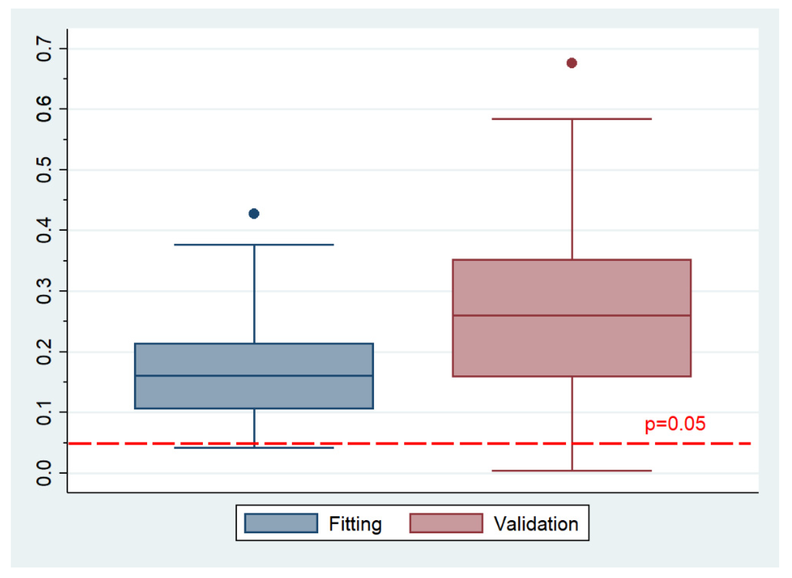
Further, as regards the goodness of fit of the two models, according to Pearson’s χ
2 results, the fitting model was rejected in only 2% of the iterations and the validation model in approximately 5% of the iterations. This is also evident in
Figure 1, according to which the models could not be rejected in almost any iteration.
3.2. Transferability Evaluation—Households Models
To explore the “transferability” of the pooled model to different countries and technologies (i.e., to examine whether it is possible to create a “universal” model of energy efficiency), eight different models were run for the five countries and three technologies and the results were compared based on three criteria: the estimated ROC curve areas, the goodness of fit of the models according to the Pearson’s χ2 test, and the Wald test regarding the equality of the coefficients. The dependent variable in all the models was “energy efficiency is a very important attribute in the purchasing decision” (coded “1” for “Yes” and “0” otherwise).
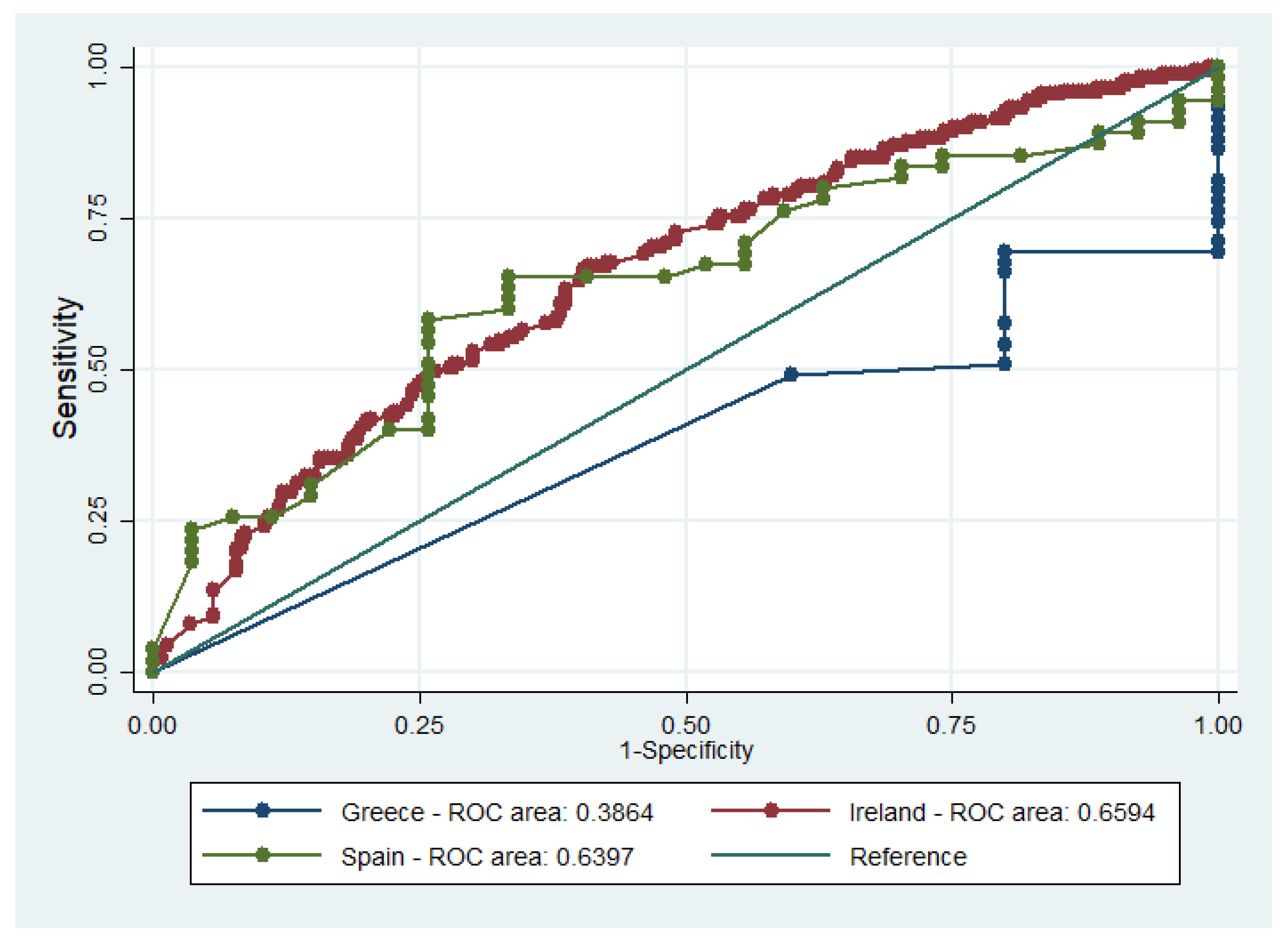
3.2.1. Country Transferability
The results for the five national subsamples are given in
Table 3 and
Table 4. In general, the calibration criterion was satisfied for all countries (yet only marginally for the Irish subsample). According to ROC comparisons, the chi-squared test yielded an average significance probability of 0.062, suggesting that there was no significant difference between the ROC areas of the five national models.
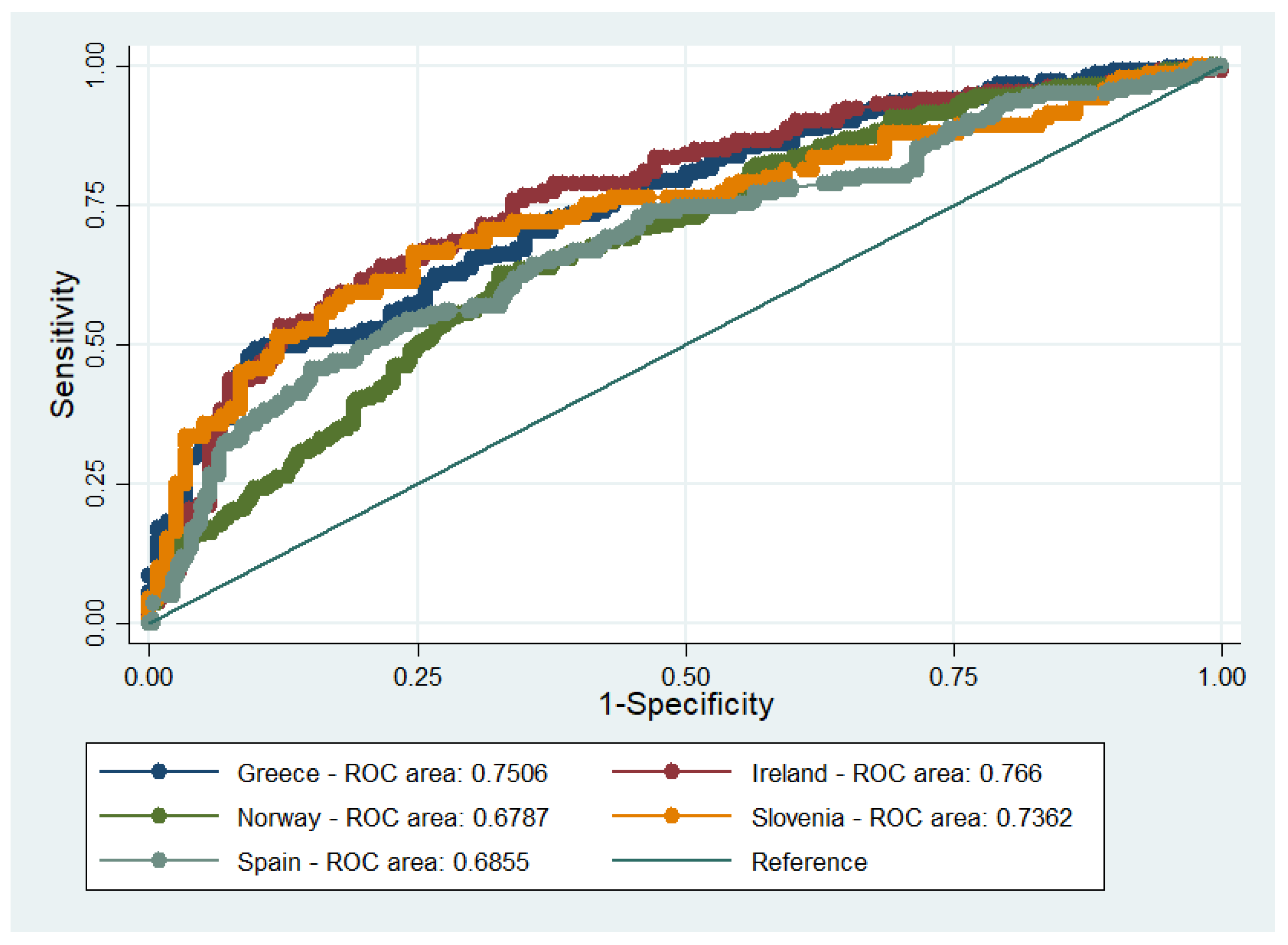
Nevertheless, the C-statistic criterion was fulfilled for three out of the five countries (
Table 4 and
Figure 2), namely, Greece, Ireland, and Slovenia. The models for Norway and Spain, although marginally, did not present acceptable discrimination.
Since the value and the statistical significance of the coefficients across the pooled and the national sub-models differed, the Wald test was implemented to test whether this difference was statistically significant. The results are given in
Table 5. The null hypothesis that all the coefficients in the examined models are equal was rejected between the pooled model and the models for Spain and Norway, as well as between the models for Spain and Norway. These results are consistent with the remarks made about the discrimination of these two models. All in all, it could be argued that the model is not transferable across all countries mainly because the importance of energy efficiency varied between the samples.
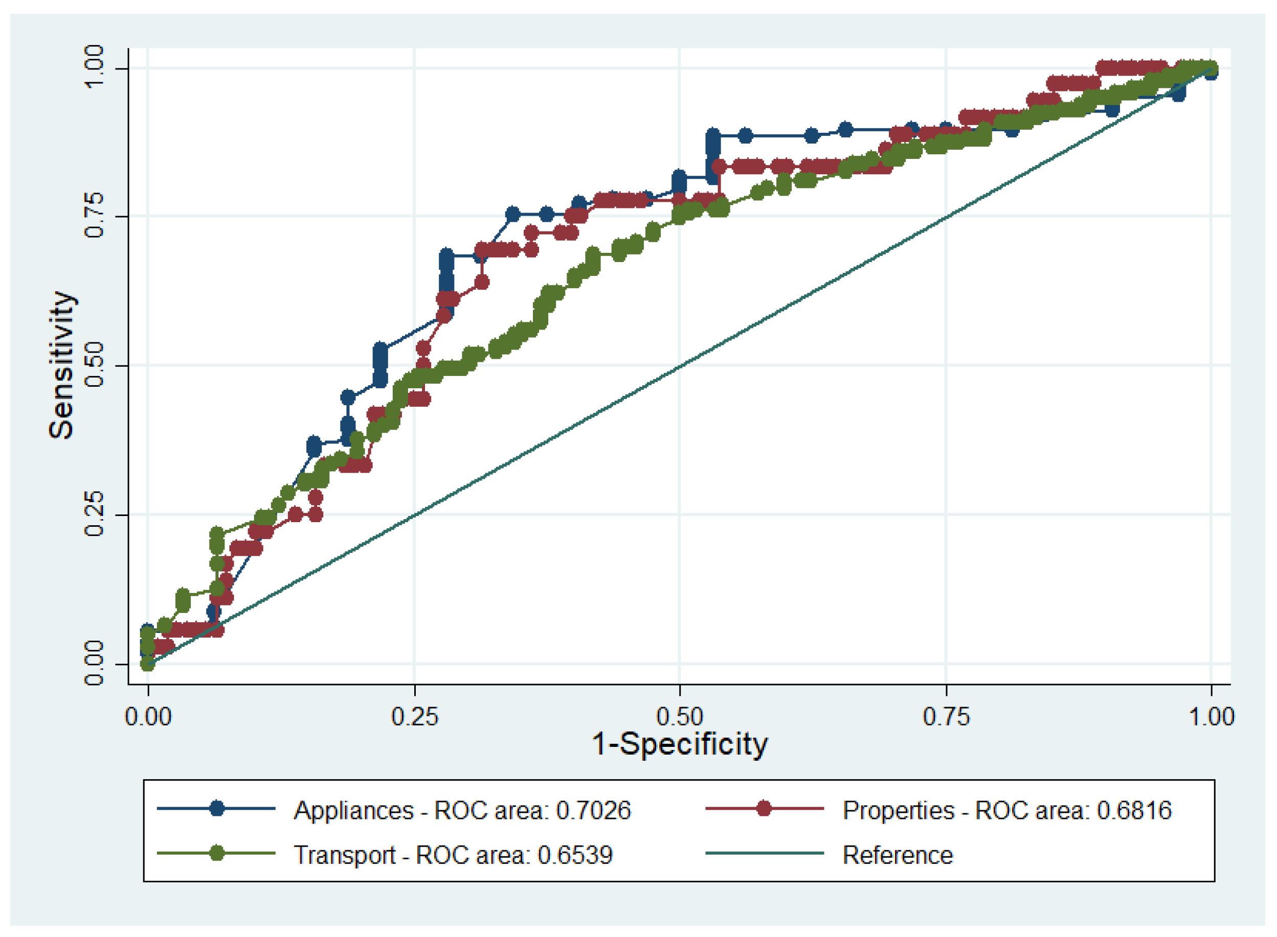
3.2.2. Technology Transferability
The results of the technological subsamples are presented in
Table 6 and
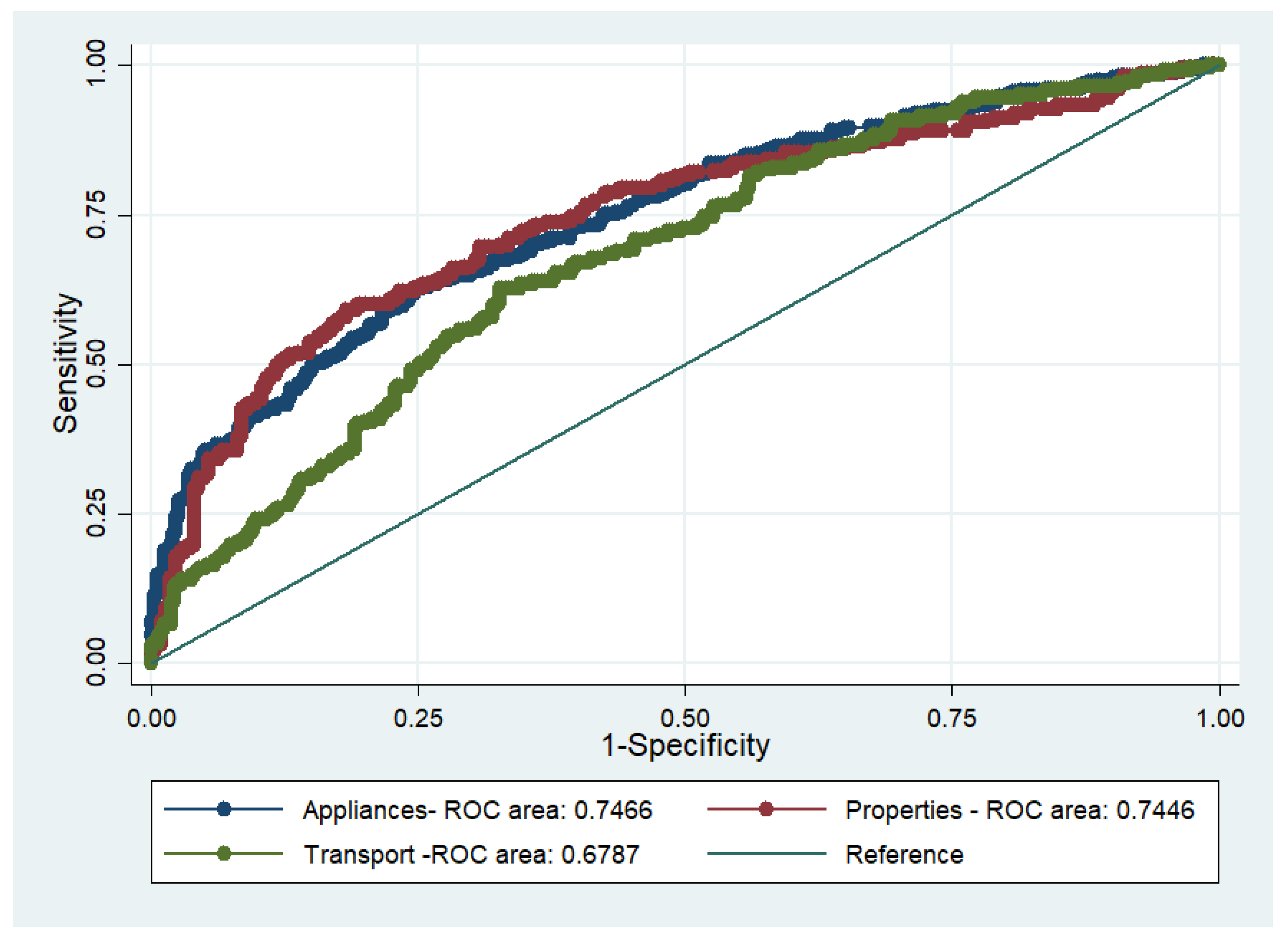
Table 7. The null hypothesis that the regression model used is the correct model could not be rejected at a 5% level (it as rejected at a 10% level for the properties model). Based on Pearson’s χ
2 test, it was suggested that there is a significant difference between the ROC areas of the three models (
p = 0.034). The test was rejected due to the transport model, which also had unacceptable discrimination given that the C-statistic was below 0.7 (
Table 7 and
Figure 3).
Finally, the “transferability” of the model was examined using the Wald test, the results of which are summarized in
Table 8. The null hypothesis that all the coefficients in the examined models are equal was rejected between the pooled model and the transport model, and between the transport model and the appliances model. Again, the Wald test results coincided with the results of discrimination for the transport model. Overall, it could be argued that the model is transferable as regards the appliances and properties models, but not the transport model.
3.3. Pooled Model Validation—FIRMS
The pooled sample for the firms included observations from Greece (appliances in services sector), Spain (appliances in services sector), and Ireland (properties and services sector and machinery in agricultural sector). The missing observations were dropped from the dataset prior to validating the pooled sample model to correctly compare the ROC curves. The final dataset contained 555 observations out of 794 (70%). Several models were run using diverse sets of predictors, which were initially selected by considering the estimated binary response models. Similarly, the dependent variable in all the models was “energy efficiency is a very important attribute in the purchasing decision” (coded “1” for “Yes” and “0” otherwise).
Table 9 presents the marginal effect of the factors affecting the probability of considering energy efficiency a “very important” attribute in the pooled sample.
According to the model, the marginal effect at the means (MEM) for those who strongly agreed that acquiring more energy-efficient equipment would reduce their firm’s environmental impact was 6.7% (i.e., on average they were about 7% more likely to value energy efficiency as “very important”). The MEMs for those who were willing to implement new energy-efficient technologies and had a good understanding of energy savings were 7.8% and 10.0% more likely to rate energy efficiency as “very important,” respectively. Further, respondents who claimed that the lack of access to loans acts as a barrier to energy investments also believed that energy efficiency is a very important attribute (MEM: 4.6%). Finally, interviewees who claimed that energy labels would affect their choice were 4.7% more likely to value the energy efficiency attribute as “very Important”.
The pooled model was tested for validity using the process described in
Section 2.2. The results for the distribution of each of the performance measures for the fitting and validation samples are summarized in
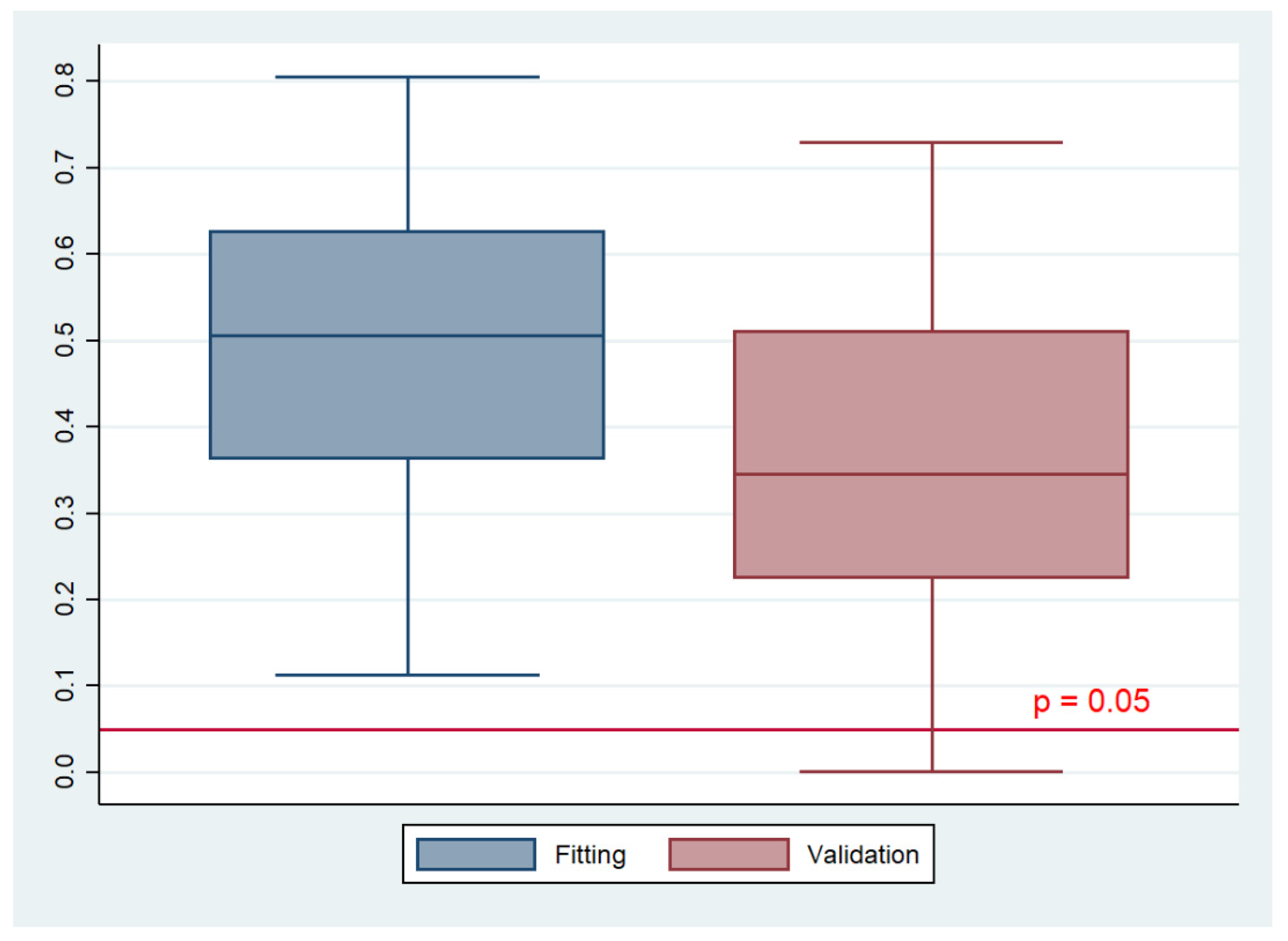
Table 10. Based on the ROC comparisons results, the chi-square test yielded an average significance probability of 0.565, which suggests that there was no statistically significant difference between the fitting and validation model ROC areas. The null hypothesis, i.e., the areas under the ROC curves are equal, was rejected in 3% of the iterations. Thus, it can be argued that the model discriminates very well. With regards to the goodness of fit of the two models, according to the Pearson’s χ
2 results the fitting model was not rejected in any of the iterations and the validation model was rejected in 2% of the iterations. Furthermore, as illustrated in
Figure 4, the models could not be rejected practically in any of the iterations.
3.4. Transferability Evaluation—Firm Models
The “transferability” of the firms’ pooled model was also tested for different countries, technologies, and sectors. In total, eight different models were run for the three countries, three technologies, and two sectors, which were compared using the three criteria, i.e., the estimated area of ROC curves, the goodness-of-fit of the models according to the Pearson’s χ2 test, and the Wald test regarding the equality of the coefficients. The dependent variable in all the models was “energy efficiency is a very important attribute in the purchasing decision” (coded “1” for “Yes” and “0” otherwise).
3.4.1. Country Transferability
The results for the three national subsamples are given in
Table 11 and
Table 12. The calibration criterion was generally satisfied for all countries. As far as the C-statistic criterion is concerned, however, none of the models presented acceptable discrimination (see
Table 12 and
Figure 5). Especially in Greece, the ROC curve area indicated a model that has negative discrimination, i.e., it is worse than random.
Since the national models failed to provide adequate discrimination, no further tests were carried out. All in all, it could be argued that the model is not transferable across countries. However, this conclusion should be seen with caution owing to the small number of observations in the cases of Spain and Greece.
3.4.2. Technology Transferability
The results for the three technological subsamples are given in
Table 13 and
Table 14. The calibration criterion was generally satisfied for all countries; therefore, the null hypothesis that the logistic regression model used is the correct model could not be rejected at a 5% level. Based on Pearson’s χ
2 test, it is suggested that there was no difference between the ROC areas of the three models (
p = 0.729) (
Table 15 and
Figure 6). However, the predictive power of the appliances model was barely acceptable.
Although the discrimination of the models was not satisfactory, the “transferability” of the model was examined by employing the Wald test (
Table 15). The null hypothesis was rejected between the pooled model and the transport model, just like in the household survey. Therefore, it could be argued that the model is transferable as regards the appliances and properties models, but not for the transport model. Yet, as mentioned, the models had weak predictive power.
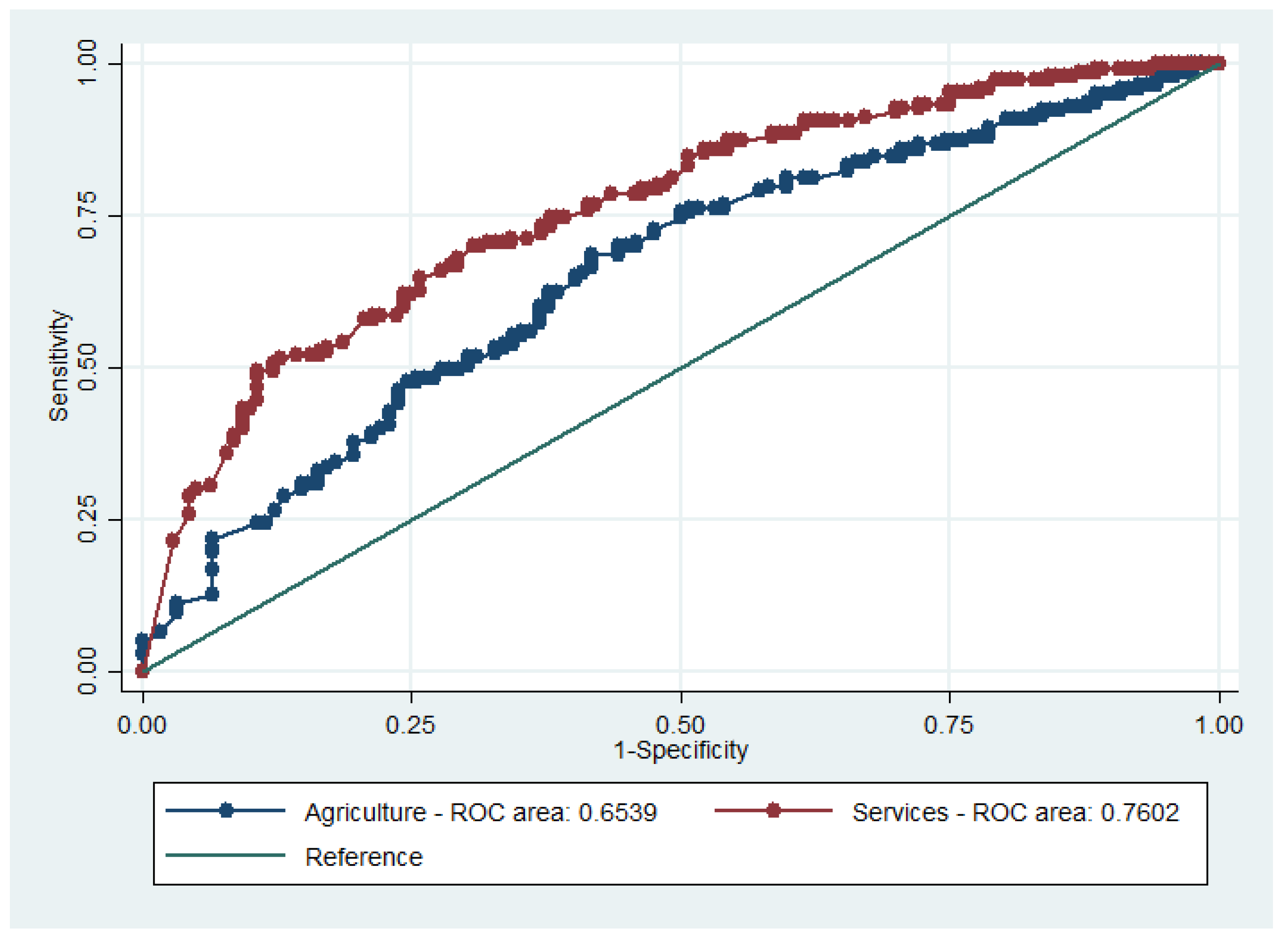
3.4.3. Sector Transferability
The “transferability” of the model was finally tested using the sectoral subsamples (i.e., agriculture and services). The results are presented in
Table 16 and
Table 17. The calibration criterion was satisfied for both sectoral models, (i.e., the hypothesis that the correct model is used could not be rejected). Based on Pearson’s χ
2 test, the null hypothesis that there is no difference between the ROC areas of the two models was rejected (
p = 0.015). Furthermore, only the services model showed an acceptable C-statistic value (
Table 17 and
Figure 7). The “transferability” of the model was examined by means of the Wald test (
Table 18). The null hypothesis was rejected for all pair comparisons. Therefore, it can be concluded that the model is not transferable across sectors.
4. Conclusions
So far, several research efforts have been carried out to investigate the role of socioeconomic characteristics and behavioral and market biases on energy efficiency investment decisions. Despite this wealth of information, however, the transferability of the results between countries or sectors remains unexplored. This is an important shortcoming because the demand for evidence-based energy policymaking is high. Too often, though, the policymakers must rely on previous studies to obtain reliable and comparative data and formulate policies at a new site, since the cost of generating new evidence for policy sites is prohibited. Since the 2000’s this is the task of the emerging field of policy transfer [
60], which aims at approximating the policy variables at a new site (policy site) by using the estimated values at a different but similar area, region or country (study site) [
61]. In all areas of policy transfer though, the transferability of policies between countries has received limited attention [
39,
62,
63], and this stands also for the energy policy field [
39,
40].
Aiming to fill this gap and addressing the inherent difficulties in cross-country policy transfer, this study applied state-of-the-art econometric techniques to complement the mostly qualitative [
60] methodological tools of policy transfer. To this end, the generalizability of the theoretical and econometric models developed in the context of the H2020 CONSEED project for investigating behavioral anomalies in EU energy efficiency was tested. The surveys were designed in a harmonized way to facilitate subsequent data pooling where possible. Specifically, two homogenized datasets for validation purposes and evaluation of the “transferability” of the models across different countries, technologies, and sectors were constructed. To the authors’ knowledge, this is the first attempt to examine whether the relationships between energy efficiency-related attitudes, sociodemographic characteristics, and potential market and non-market failures are general or attributable only to a narrow set of conditions. The novelty of our approach lies with (1) providing a robust statistical specification of heterogeneity in the consumer, technology, and sector space and (2) understanding in a quantitative, statistical sense the limitations of lesson drawing in a policy transfer exercise. The main conclusions drawn from the statistical process are discussed hereinafter.
According to the C-statistic—a measure of the predictive power of the model—and Pearson’s χ2 goodness-of-fit statistic—a measure of calibration of the model—the regression model used was the correct one; the pooled models derived for the households and the firm samples passed the internal validation tests (that is, Proposition 1 was verified). Further, given the larger number of observations and the diverse nature of the population, the pooled samples seemed to allow for a more reliable investigation of the relative importance of the factors influencing consumers’ attitudes and beliefs towards energy investment decisions.
Our results show that energy efficiency importance varied across products and countries. For instance, in household appliances, energy efficiency was among the top two factors (more than 70% rated it as very important), whereas energy efficiency for cars was ranked only fourth. For this reason, and as expected from the relevant literature, the transferability of the results (i.e., the use of a “universal” model of energy efficiency from the pooled model), across countries, technologies, and sectors is limited. This was confirmed by the statistical tests used to determine transferability (i.e., Proposition 2 was rejected). Further, relatively small sample sizes for some sectors may also have contributed to low transferability.
All in all, the pooled models were validated, i.e., they were correctly specified and accurately represented the phenomena studied. Nevertheless, the extrapolation of the results to specific populations in terms of “space” (i.e., country) and “target” (e.g., sectors and technologies) should be seen with caution from a policy perspective for two reasons. First, as already mentioned, the transferability of the models proved to be limited owing to the plethora of parameters influencing energy efficiency-related attitudes and behavior. This finding is consistent with the results of previous research. For instance, Wang et al. [
38], who compared seven data-driven models to forecast electricity usage at a city-scale level, concluded that the models can predict the city-level electricity demand well but their generalizability is in question. Miller [
36] used machine learning modeling approaches in building energy prediction and found that no single modeling technique produces accurate results for all the different types of buildings. Hopf et al. [
35] used machine learning models to investigate, among other things, whether a model trained on one geographic region can be transferred to another geographic region. The authors claimed that the model can be transferred “…with acceptable performance loss…” Nevertheless, when they tested whether data from one company can improve the predictiveness of the model of another company, they noticed that “…no performance improvement was possible…” Finally, Martinez-Soto and Jentsch [
37], who developed and tested a transferable residential energy model, found that their model could predict the final energy demand of the residential sector of different countries. Yet, they noticed that the model relies only on six input parameters and, thus, it was not possible to check the effect of detailed energy efficiency measures that could be implemented in a country. Second, one cannot exclude the possibility of endogeneity, i.e., the correlation of an explanatory variable in the regression model with the error term in the model [
64,
65,
66]. Two cases are especially common in social research: (1) when important variables are omitted from the model (called “omitted variable bias”) and (2) when the dependent variable is also a predictor of an independent variable (known as “simultaneity bias” or “reverse causality”) [
65]. A common method for dealing with endogeneity is the use of instrumental variables, but in cross-sectional surveys and with few variables, like in our case, it is practically impossible to handle endogeneity [
65]. Similarly, controlling for all sources of variance in the context of social science is not feasible, i.e., it is not possible to include all possible sources of variance of a dependent variable in the regression model from a practical viewpoint [
64]. For this reason, and even though all surveys were based on randomized samples, a design that assures the causal inference [
64,
67] endogeneity may still be an issue (i.e., those who believe that “energy efficiency is a very important attribute in the purchasing decision” may also be more affected by the energy labels, i.e., the two variables are simultaneously causing each other, and this may bias the results upwards as well as downwards). To provide more consistent answers, future research surveys need to collect different subsamples for each country and for several products that will allow international and intersectoral comparisons.


 ,
, 


