
Analysis of Synthetic Voltage vs. Capacity Datasets for Big Data Li-ion Diagnosis and Prognosis


Hawaii Natural Energy Institute, University of Hawai̒i at Mānoa, Honolulu, HI 96822, USA
*
Author to whom correspondence should be addressed.
Energies 2021, 14(9), 2371; https://doi.org/10.3390/en14092371
Submission received: 18 March 2021
/
Revised: 16 April 2021
/
Accepted: 19 April 2021
/
Published: 22 April 2021
(This article belongs to the Special Issue Battery Management for Electric Vehicles)
Abstract
:The development of data driven methods for Li-ion battery diagnosis and prognosis is a growing field of research for the battery community. A big limitation is usually the size of the training datasets which are typically not fully representative of the real usage of the cells. Synthetic datasets were proposed to circumvent this issue. This publication provides improved datasets for three major battery chemistries, LiFePO4, Nickel Aluminum Cobalt Oxide, and Nickel Manganese Cobalt Oxide 811. These datasets can be used for statistical or deep learning methods. This work also provides a detailed statistical analysis of the datasets. Accurate diagnosis as well as early prognosis comparable with state of the art, while providing physical interpretability, were demonstrated by using the combined information of three learnable parameters.
1. Introduction
With the urgent need to reduce the emissions of fossil fuels, energy storage is going to play a key role in the future of transportation and grid services. Within all the known storage solutions, intercalation batteries appear to be good candidates for the task despite some durability and safety concerns. Li-ion battery aging is path-dependent [1,2] and distinct degradation mechanisms could be inhibited or exacerbated by different stress factors. This could drastically affect reliability and adds a lot of complexity to onboard diagnosis and prognosis. A possible way to handle this complexity is to use artificial intelligence (AI), a technique that has shown tremendous potential for improving energy storage materials [1] as well as diagnosis and prognosis [3,4,5]. For the latter, the primary challenge area is that the training data is, in most cases, not representative of the projected usage and thus does not encompass the sporadic spectrum of degradation that can occur in the field [4,6]. This might render the proposed algorithms inapplicable in deployed systems. Due to the cost associated with the gathering of experimental data, most studies that employ AI for commercial cell diagnosis or prognosis only used training datasets with under 20 samples which is not enough. Among the outliers [6,7,8,9,10,11,12,13,14], Severson et al. [6,12,15] tested 124 different conditions, although only varied the charging parameters and did not perform any reference performance testing.
While the growing online databases [6,16,17,18,19,20,21] and the newly proposed Battery Data Genome [22] are providing steps in the right direction, they are still vastly insufficient to provide enough data to cover the changes that could be associated with small differences in duty cycle [23]. This path dependence of deployed systems is a determining aspect for the validation of online diagnosis and prognosis tools [24,25] and is the largest knowledge gap in scientific data for the AI community. To circumvent this issue, we proposed the use of synthetic cycling data [26] to complement existing datasets and accelerate the development of new and unique data-driven tools by providing the community with supplementary data on a wider array of degradation paths.
This publication is building on our previous methodological work [26] where we used the mechanistic modeling approach [27,28,29,30] to generate a proof of concept dataset for a commercial graphite (Gr)/LiFePO4 (LFP) cell containing more than 500,000 unique voltage versus capacity and 125,000 different duty cycles. In this work, we refined the technique and will be offering updated datasets with five times more resolution and for additional battery chemistries. We synthesized data for a Gr//LFP cell at C/25, as an update of our previous dataset, for a Gr//Nickel Aluminum Cobalt Oxide (NCA) cell, and for a Gr//Nickel Manganese Cobalt Oxide (NMC811) cell at C/30 and C/25, respectively [31,32,33,34]. In addition to the data synthesis, we also performed a statistical analysis of the results to address early prognosability and proposed meaningful learnable parameters [15] in order to provide physical and statistical interpretability, another significant challenge areas for AI algorithms. For this purpose, we investigated the correlation of various features of interest (FOI) with state of health (SOH) [24].
A recent prospective study [22] highlighted different challenge problems necessary to accelerate the impact of AI methods on the battery field. This work is addressing tier 1 challenges. We believe our synthetic cycles can be used for diagnosis, for the determination of the minimum number of cycles to predict cycle life, and to address how well predictions can transfer from one technology to the other. In this work, degradation is defined as changes in loss of lithium inventory (LLI) and/or loss of active material (LAM). Diagnosis will be defined as a single point estimation of capacity loss, LLI, and LAM on the positive and negative electrodes (PE and NE, respectively) without prior information. SOH and prognosis will be referencing to the remaining useful life determination (i.e., how many more cycles before 20% capacity loss) and not the evolution of capacity loss. This is to take into consideration the second stage of battery degradation [6,23,35,36,37,38,39].
2. Materials and Methods
2.1. Half-Cell Data
The voltage response of commercial cells was reconstructed using half-cell data from PE and NE. The commercial cells used for this study were comprehensively studied in previous work. The Gr//NCA cell was based on the Panasonic 3350 mAh NCR 18650B batteries studied in [35,40,41,42,43]. The Gr//NMC811 cell was based on the PE from a Samsung-SDI 3500 mAh INR18650-35E battery [44] and a stock NE, and the Gr//LFP cell was based on an A123 2300 mAh ANR26650M battery [23,45]. Interested readers are referred to the original publications for more details. Since all the cells are using a Gr NE, they will be referred to by their PE only in the rest of this work.
Before being opened in an Argon-filled glove box, all the batteries were discharged to a 0% state of charge (SOC) [46]. Electrode discs (18 mm in diameter) were then punched and rinsed in a dimethyl carbonate (DMC) solution. N-methyl-2-pyrrolidone (NMP) was used to wipe the backside of the electrodes. The electrodes were tested on a multi-channel Bio-Logic VMP3 potentiostat (Bio-Logic, Claix, France) against a lithium counter electrode with a 1.0 M LiPF6 in ethylene carbonate + DMC (1:1 by weight) and 2% wt. vinylene carbonate electrolyte as well as one Whatman GF-D fiberglass disc (12.7 mm in diameter, Whatman, Kent, UK) as a separator. The complete testing protocol can be found in [46].
2.2. Simulations
The synthetic voltage vs. capacity curves concept was extensively described in [26] and will not be repeated in detail here. In our approach, we use experimental data for the PE and NE to reconstruct the electrochemical behavior of full cells aged under different degradation scenarios without the need for electrochemical equations [27,28,29,30]. Both electrodes are matched with a loading ratio (LR) that corresponds to the capacity ratio between the electrodes and an offset (OFS) that corresponds to their slippage, along with resistance and kinetic adjustments if necessary [30], Table A1.
With degradation, LR and OFS are predictably affected by the LAMs and LLI [30]. Using this knowledge, the LAMs and LLI can be varied and the projected changes of LR and OFS, and thus the full-cell electrochemical response, can be calculated without the need for knowledge of the conditions leading to this degradation. In our initial dataset, more than 5000 combinations of LAMs and LLI were computed, each up to 85% of each degradation mode with 0.85% intervals [26]. To better visualize the impact of the degradation, only the C/25 charges were calculated. This is equivalent to performing a reference performance test at a given SOH and at room temperature. In addition, to test different duty cycles, more than 125,000 different evolutions of LAMs and LLI values were calculated from predetermined equations involving linear and exponential evolution for each degradation mode, delayed exponential acceleration for LLI, and different reversibilities for lithium plating (see Appendix A). Since the publication of our proof-of-concept synthetic datasets [26], we and others have utilized the data for different purposes and found that some of the features could be improved. This publication addresses some of the improvements.
The initial datasets provided 201 points for each voltage vs. capacity (V vs. Q) curve (1 point every 0.5% capacity) and the step was set at 0.85% of each degradation mode. This proved problematic to simulate early cycles for duty cycles with low degradation. In such cases, multiple cycles were using the same V vs. Q curve leading to the prediction of no voltage variations and constant capacity. To solve the problem, the resolution of the data was increased to 0.1% capacity (1001 points per voltage vs. capacity curves) and the step for the degradation was changed to non-constant with a resolution multiplied by 10 between 0 and 2% degradation, by 4 between 2.25% and 5%, and by 2 between 5 and 15% degradation. Overall, this added 38 simulations per path which increased the number of V vs. Q curves in the V vs. Q matrix by almost 200,000 to more than 700,000.
Increasing the number of points by 500% and the number of simulations by 35% increased the size of the V vs. Q matrix from roughly 500 MB to 6 GB. This was later halved by changing the floating-point numbers precision from double to single. This did not alter the quality of the data since only three decimals are needed to reach the mV resolution of the initial half-cell data. The increase in the number of points per voltage curve was however more problematic for the duty cycle dataset which contained more than 3,000,000 V vs. Q curves (>125,000 duty cycles with one V vs. Q curve every 100 cycles for 3000 cycles) and was already above 3 GB in the proof-of-concept data. This issue was solved by pushing our initial concept further. As explained in [26], and to avoid lengthy calculation time, the duty cycle data was not calculated but harvested from the V vs. Q matrix by finding the V vs. Q curve with the closest mix of LLI and LAMs to the one to simulate. In the new version of the duty cycle matrix, only the index of the V vs. Q curve is harvested which precludes the need for a large array and reduced the dataset size from 3 GB to only 15 MB for 125,000 duty cycles. This now allows to simulate duty cycle datasets two orders of magnitude larger for the same file size. In this work, we limited the new data to an increase of the cycle resolution by offering data with 10-cycle intervals up to 200 cycles. Coupled with the higher resolution of the voltage vs. capacity curves, this allows to visualize well-defined changes early in the duty cycle prediction, an essential feature for early prognosis. This should offer more possibilities for the development of early prognosis tools. All the datasets synthesized in this work are freely available for download [31,32,33,34].
2.3. FOI Definition and Selection
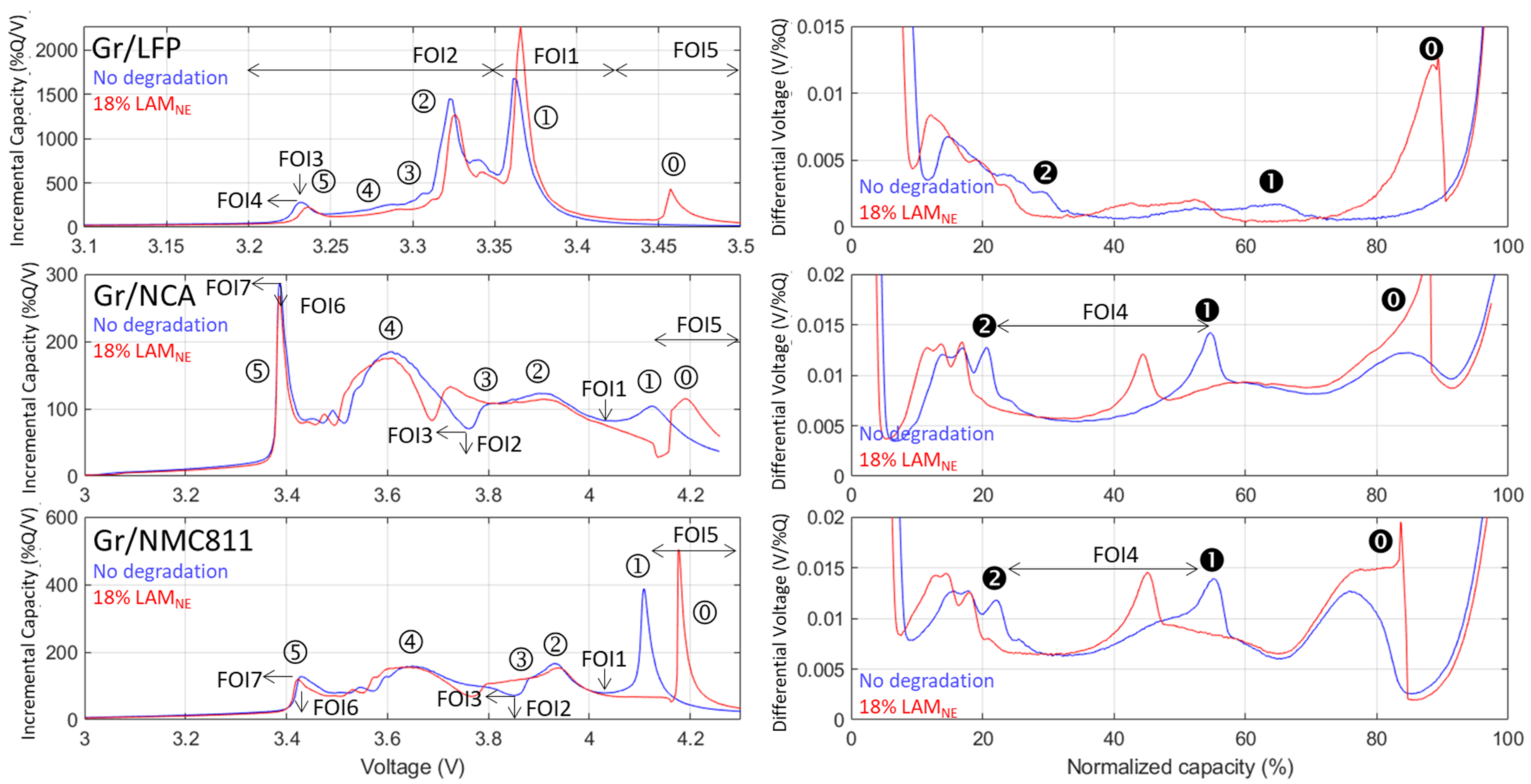
Figure 1 presents the incremental capacity (IC) and differential voltage (DV) curves associated with the three chemistries at two different SOHs. Based on our previous analysis of the changes of voltages associated with degradation, FOIs were defined for each chemistry, Table A3.
For the LFP simulations, the area under peak ① was used as FOI1, the area under peaks ② to ⑤ as FOI2, the position and intensity of peak ⑤ as FOI3 and FOI4, and the area under peak ⓪ as FOI5. This should provide information on LLI plus LAMNE (FOI1), LAMNE (FOI2), LAMPE (FOI3 and 4), and reversible lithium plating (FOI5) [23,45].
For the NCA and NMC cells, the intensity of the minimum between peaks ① and ② was used as FOI1, the position and intensity of the minimum between peaks λ and ➃ as FOI2 and FOI3. FOI4 was defined as the capacity difference between peaks ➊ and ➋ on the DV curves. FOI5 was defined as the area under peak ⓪ and the position and the intensity of peak ⑤ will be used as FOI6 and FOI7. Based on our previous work [35,40,41,42,43], FOI1 should be representative of LAMPE, FOI4 of LAMNE, and FOI5 of reversible plating.
Diagnosis with physical integrability is calculated from single FOIs and from the combined variations of three FOIs following the palapala-aina method we proposed in 2017 [24] in which the evolution of three FOIS are combined in a 3D map with a 100 × 100 × 100 mesh. The mesh size for each FOI is indicated in Table A3.
3. Results
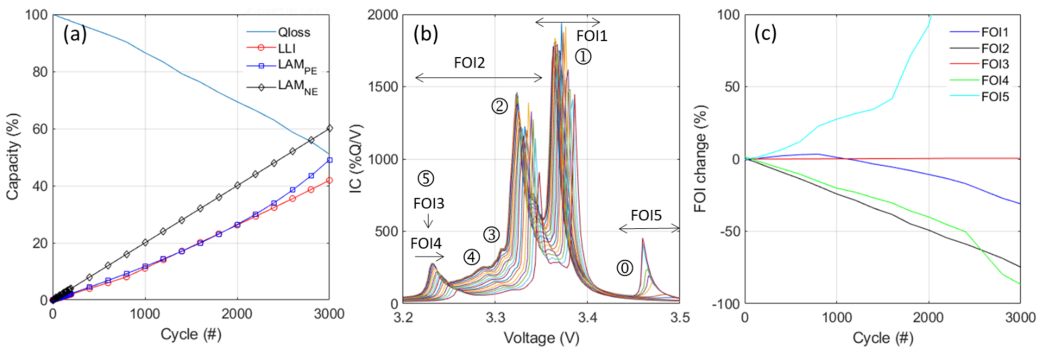
Figure 2 presents an example of one of the more than 125,000 duty cycles provided for the LFP cell (#20050). In this example, LAMNE is the main degradation mode. Looking at the evolution of the associated IC curves, Figure 2b, peak ① intensity increased before plateauing and decreasing, whereas peaks ② to ⑤ only decreased. This was expected for a degradation involving more LAMNE than LLI [23,30]. The peak position also shifted towards higher voltages because of a polarization increase associated with the increase of the local current density (same current on less active material). Moreover, because LAMNE was higher than LLI, plating started to occur and the peak ⓪ started to grow [23,30].
The chosen FOIs, Figure 2c, accurately tracked the changes in the IC curve as FOI1 increased before decreasing, FOI2 and FOI4 decreased, and FOI3 and FOI5 increased. However, it must be noted that FOI4 lost accuracy after 2200 cycles. This is because of its definition; FOI3 was defined as the maximum intensity between a limited potential range (3 and 3.25 V, Table A3) in order to catch the intensity of peak ⑤ without englobing peak ④. With the increase of the polarization, the peak was shifted to a potential larger than 3.25 V and its intensity can therefore no longer be tracked. This is a common limitation for FOI tracking and it needs to be taken into consideration when choosing learnable parameters [24]. This highlights that more work is needed for automated FOI tracking. In this work, we hope to avoid this issue as much as possible by focusing our effort on the diagnosis and early prognosis based on cycles 10, 50, 100, 200, 400, and 1000.
3.1. FOI vs. Diagnosis
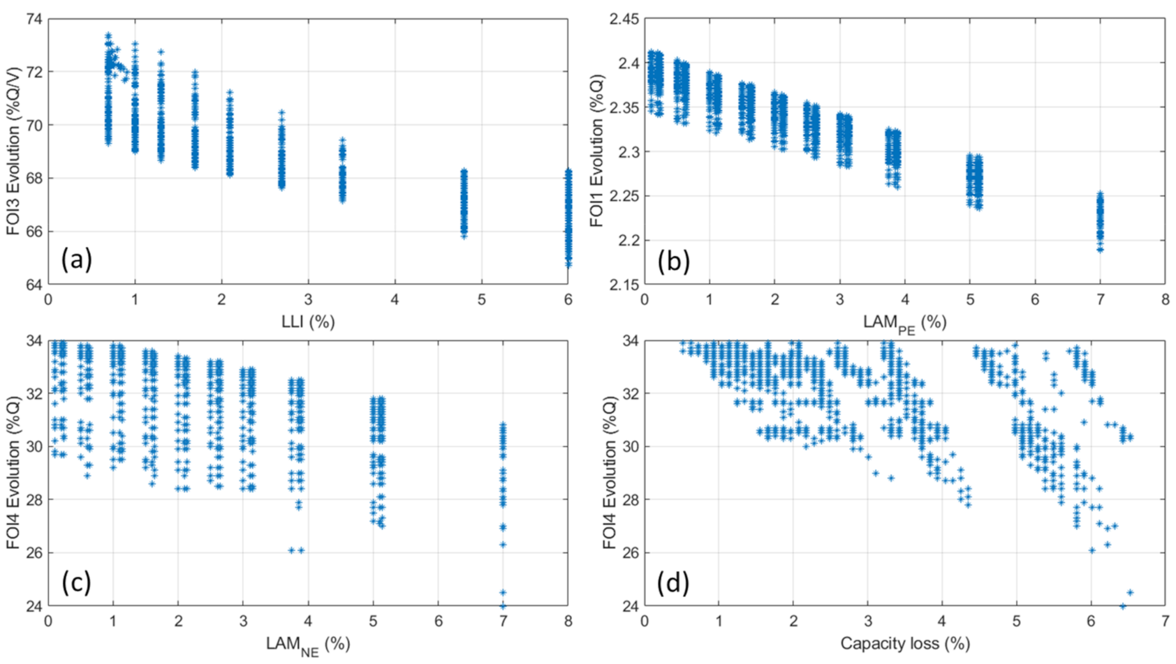
Based on our previous studies on the commercial cells used in this work [23,35,40,41,42,43,44,45], some FOIs were already established to provide good a diagnosis over the tested experimental conditions. For the LFP cell, FOI1 was shown to be sensitive to LLI and LAMNE, and FOI2 changes were found to be correlated to LAMNE. For the NCA and NMC811 cells, FOI1 was shown to be representative of LAMPE and FOI4 of LAMNE. Using the synthetic cycles, the potential of those FOIs over a wider range of conditions can be tested.
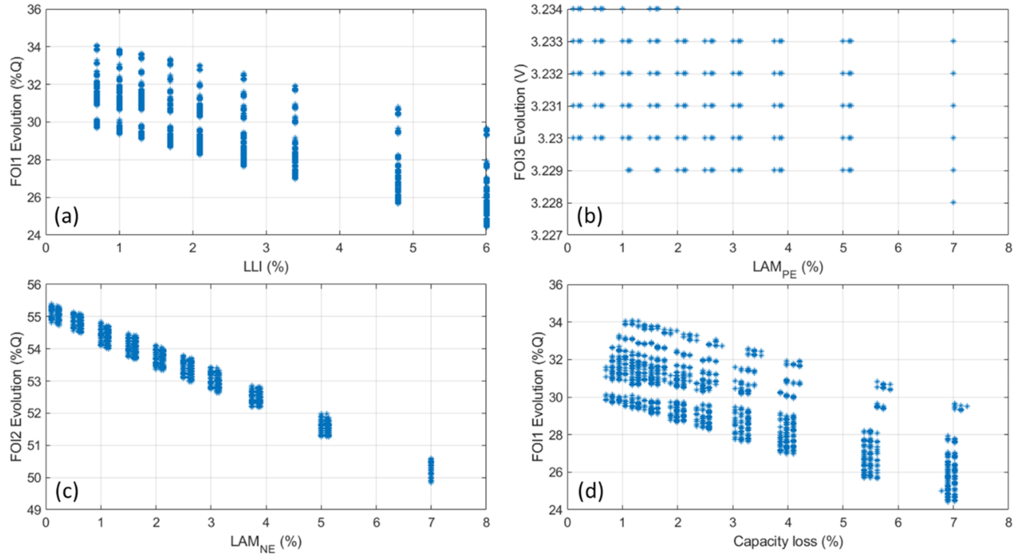
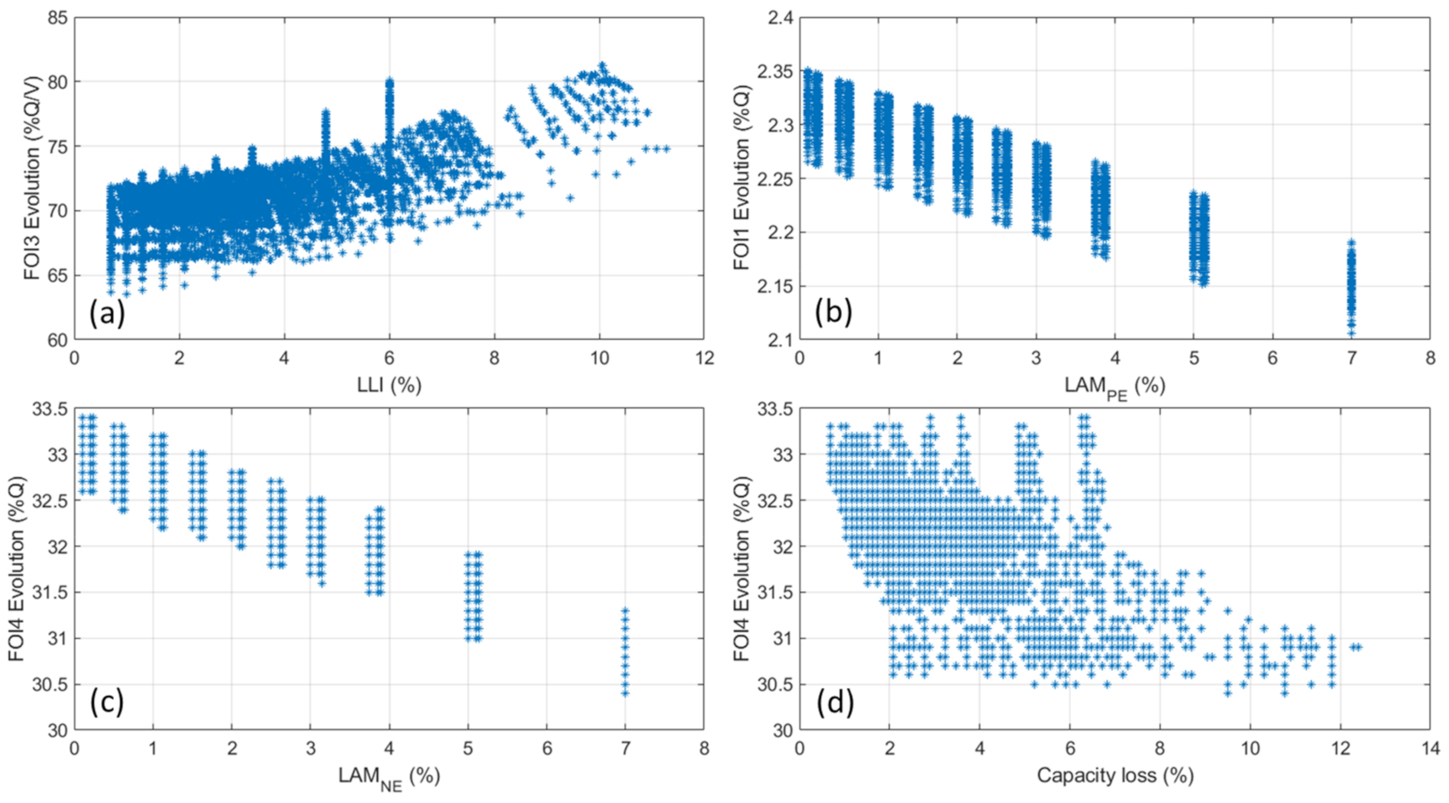
As expected [24], although they were valid choices in the aforementioned studies, their applicability for diagnosis cannot be extended to all the possible aging conditions. Table 1 summarizes the correlation coefficient between the different FOIs and the percentage of LLI, LAMPE, LAMNE, and the capacity loss at cycle 100 for the LFP cell. Figure 3 showcases the associated evolution of the most adapted FOI for all four components of the diagnosis at cycle 100 for each duty cycle. As expected, FOI1 is sensitive to both LLI and LAMNE with Pearson correlation coefficients ρ of −0.74 and 0.62. It also has a relatively high correlation with capacity loss (−0.72) which is not surprising since capacity loss is usually induced by LLI [25] in graphite-based cells. However, even if the correlation is rather high, Figure 3a,d showcases that FOI1 cannot be used for LLI or capacity loss diagnosis as the distribution is broad (close to ±10% around the average). For LAMNE, while all FOIs have absolute correlation coefficients with LAMNE above 0.6, FOI2 is, as expected, the best choice with a correlation coefficient of −0.99, Figure 3c. For LAMPE, the best FOI seemed to be FOI3 with a ρ equal to −0.36 but Figure 3b showcases that the peak voltage shift was small, and that sub millivolt accuracy would be necessary to take advantage of this FOI.
For the NCA and NMC811 cells (Appendix B, Table A4, Table A7, Figure A1, Figure A5), FOI1 was found to be the most representative of LAMPE (ρ > 0.95) and FOI4 of LAMNE (ρ = −0.64 for NCA and −0.96 for NMC811) as expected. For LLI, FOI3 seemed the most adapted (ρ = −0.89 for NCA and 0.63 for NMC811). For the capacity loss, the best FOI seemed also to be FOI4 with ρ of ~0.5 but the overall correlation is rather small.
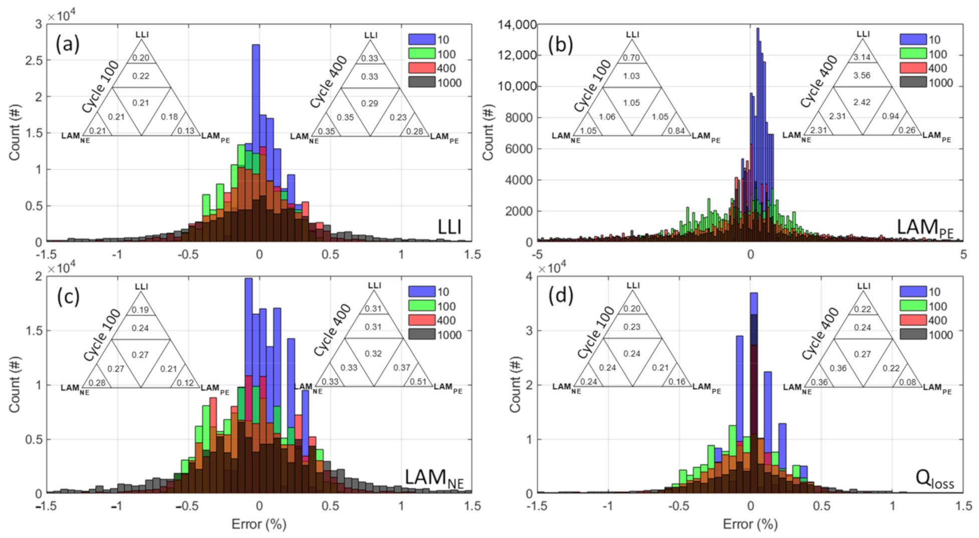
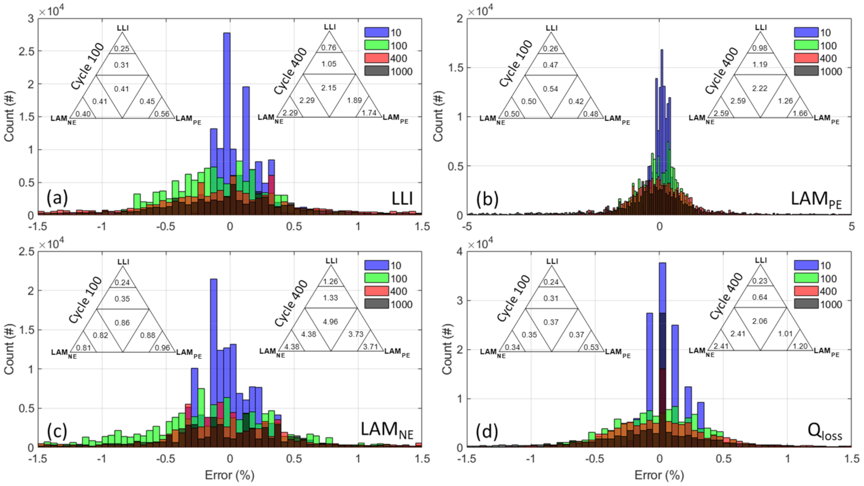
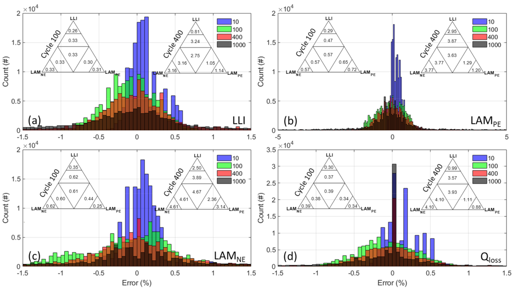
Table 1 also showcases the correlations associated with considering three FOI together, as proposed in [24]. Using this technique and FOIs 1, 2, and 4, correlation coefficients over 0.99 were obtained for LLI, LAMNE, and the capacity loss with a coefficient of 0.8 for LAMPE. For the NCA and NMC811 cells, the same combination of FOIs gave correlation coefficients of 0.89 or above for all four components (Appendix B, Table A4 and Table A7). Table 2 presents the mean estimation errors for LLI, LAMPE, LAMNE, and the capacity loss at cycles 10, 50, 100, 200, 400, and 1000 for the LFP cell using the three FOI together. The same data is plotted as histograms in Figure 4. The mean diagnosis error for more than 125,000 duty cycles was always below 0.8% and the standard deviations were found to increase with the cycle number while they were all below 1% except for LAMPE up to cycle 400. The inset in Figure 4 presents the standard deviations for different mixes of degradation at cycles 100 and 400 plotted on a ternary diagram in order to visualize the impact of the degradation mix on the accuracy of the approach. Overall, the standard deviations are rather homogeneous over the entire spectrum of degradation although they seem slightly lower for high LLI ratios and surprisingly high for LAMPE except for LAMPE estimation after 400 cycles where high LLI has more deviation. Table A5 and Figure A2 as well as Table A8 and Figure A6 in Appendix B present the same analysis for the NCA and NMC811 cells, respectively. The results are similar with average errors below 1% even at cycle 1000 except for LAMNE in the NCA cell which is above 1% only after 1000 cycles. The calculated standard deviations were slightly higher than those of the LFP cell but were always below 10%. Looking at the insets, the distribution of the standard deviations at cycles 100 and 400 are smaller for the degradation with a high percentage of LLI in the degradation mix and worst for high LAMPE for the NCA cell and high LAMNE for the NMC811 cell.
3.2. Learnable Parameters vs. Early Prognosis
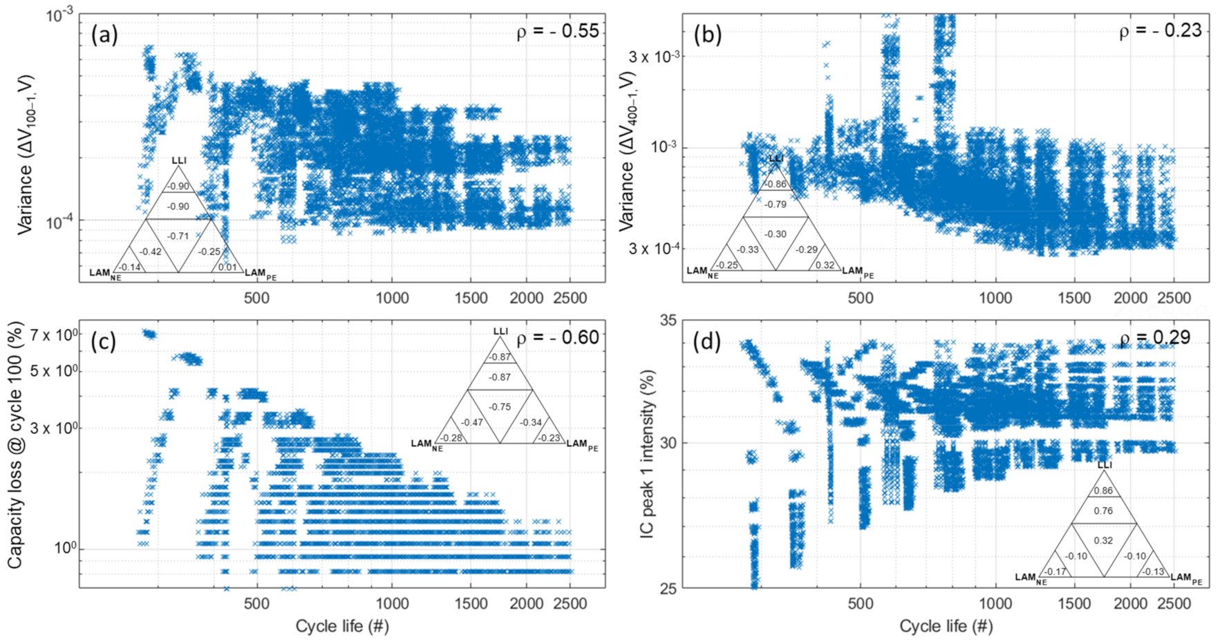
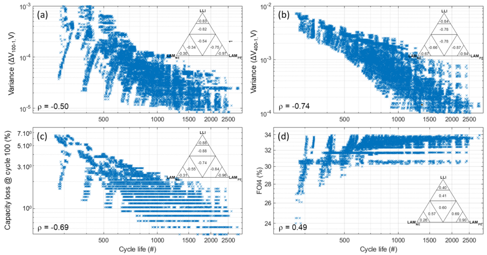
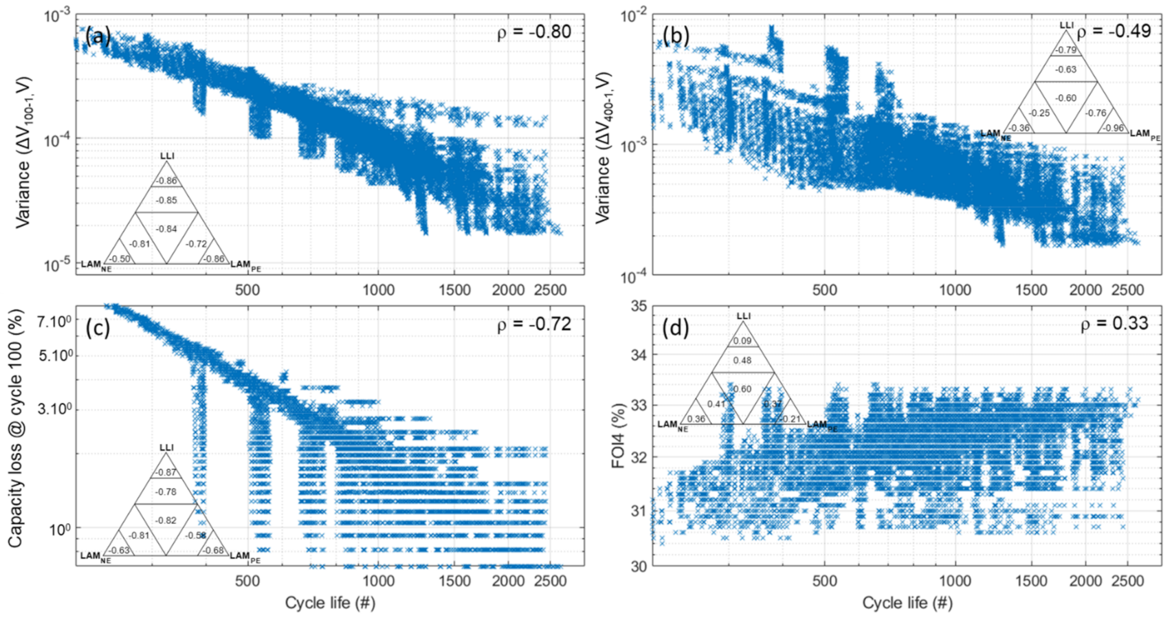
AI algorithms often rely on learnable parameters to reduce the complexity of training the algorithms and a lot of different parameters were proposed in the literature. Although some studies seem to fit the full constant current voltage data [47], most studies focused on a specific part of the electrochemical response such as the resistance [11,48,49,50,51,52], the curvature of the capacity evolution [53,54], the capacity of a specific section of the voltage response [9,55,56,57], electrochemical impedance spectroscopy [58,59,60], the variance of the voltage response [6,12], or electrochemical voltage spectroscopies [47,61,62,63,64,65,66,67,68,69,70,71,72]. In this work, we focused on the variance, the capacity loss, and the FOI most sensitive to capacity loss. Figure 5 presents the relationship of the variance between cycle 100 and cycle 1, the variance between cycle 400 and cycle 1, the capacity loss at cycle 100, and of FOI1 at cycle 100 with the end-of-life cycle (i.e., the cycle at which the capacity loss reached 20%) for the LFP cell. Figure A3 and Figure A7 in Appendix B present the same results for the NCA and NMC811 cells, respectively. The correlations are summarized in Table 3. The insets showcase the correlation coefficient for specific degradation paths.
Overall, the variance between cycles 100 and cycle 1 is not a great indicator of EOL with correlations between −0.55 (LFP) and −0.80 (NMC811) whether calculated on the voltage (V100–V1) or the capacity (Q100–Q1, lower correlation, not shown). However, the correlation coefficients are much higher (ρ > 0.9) for duty cycles with a high LLI ratio. The lowest coefficients are observed for duty cycles with high ratios of LAMPE or LAMNE. The difference between our results and the literature [6,12] could be explained by the broader testing conditions but also by the difference in rate. Our results were obtained from C/25 charges whereas 4C discharges were used in the literature [6,12]. At 4C, changes in polarization will induce more changes than at C/25 which would likely change the correlation. Similar results can be observed for the three other tested parameters. Overall, strait capacity loss is the best indicator closely followed by the variance between cycle 100 and cycle 1. It has to be noted that the correlation coefficients for the capacity loss are higher than reported in the literature for smaller datasets (~0.5) [73,74].
4. Discussion
4.1. Diagnosis
The diagnosis obtained by using the method proposed in [24] could be considered successful with average errors almost all below 1% when tested on more than 125,000 duty cycles, up to 1000 cycles and on three chemistries. Compared to our previous work [26], a better definition of the FOI for the LFP cell improved the LAMPE estimation but this diagnosis will always be difficult for LFP cells because of the flat voltage response. LAMPE estimation is much easier for NCA and NMC811. This work pushed the analysis of the results deeper than in [26] and the standard deviations were studied on various subsets of the entire degradation path matrix from high LLI to high LAMPE and LAMNE ratios or a mix of everything. It was found that slightly lower standard deviations were observed for high LLI as well as high LAMPE for LFP and NMC811 and high LAMPE for NCA, although the differences were small at cycle 100. At cycle 400, the standard deviations are higher and the differences between the different degradation mixes are more visible. Overall, the method can be considered robust and applicable to multiple chemistries.
4.2. Early Prognosis
For early prognosis, this study confirmed our previous observations [26] that some of the proposed learnable parameters might not be valid on the entire spectrum of possible degradations. Surprisingly, the best indicator overall seems to be simply the capacity loss but the correlation is still much lower than needed (ρ ~ 0.6–0.8) to have full confidence in the early prognosis. However, a closer analysis showed that the correlation is highly dependent on the mix of degradation and that degradation with a high share of LLI seems to be more predictable using the proposed learnable parameters or capacity loss (ρ ~ 0.8–0.9). This highlights that the synthetic cycles are offering information that would be difficult to obtain experimentally. It could also be argued that they might have the opposite problem than that of the literature by covering too broad of a degradation panel compared to what is possible in real life. However, the technique is still young, and the equations used to generate the duty cycles could be tuned to reflect more real life, especially since the improved approach for duty cycle generation now allows to simulate more cycles. The results of the experimental design proposed as the Tier 2 challenge of the battery data genome [22] as well as access to more field data would be invaluable to define limits on the conditions to scan. In the meantime, we still believe our synthetic cycles are a transformative solution to prospect for meaningful early diagnosis and prognosis indicators, whether for statistical or deep-learning data-driven methods.
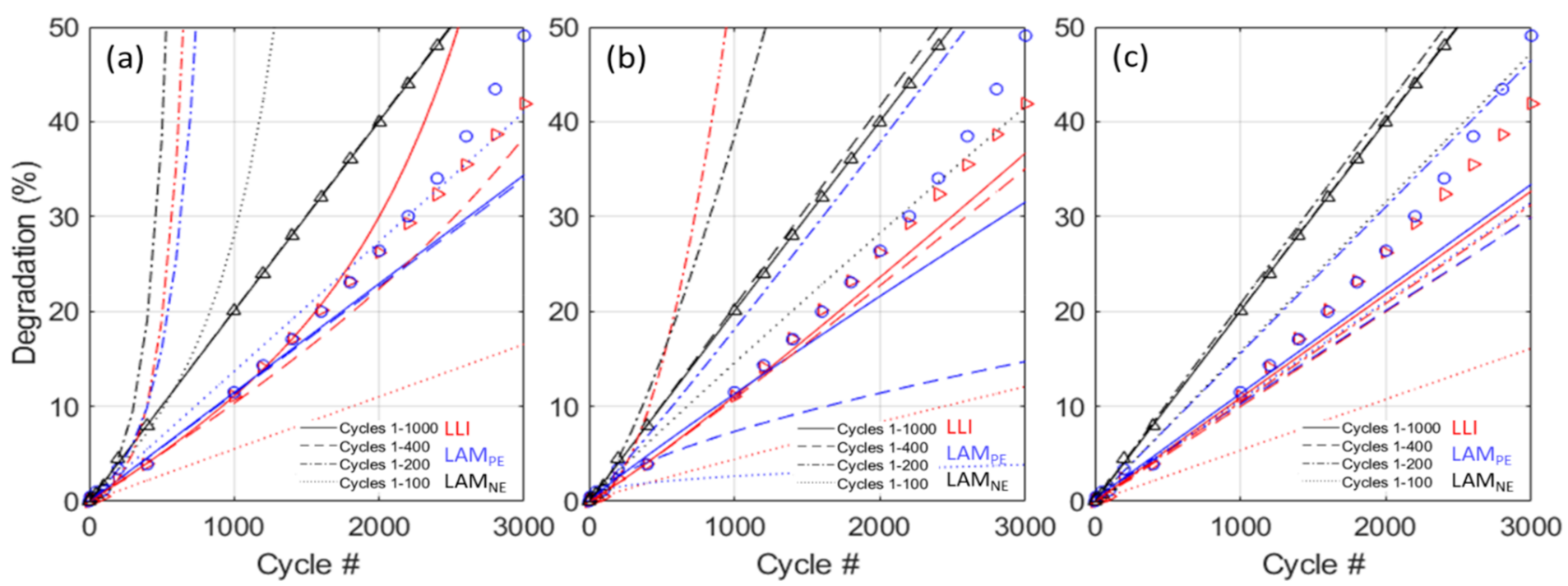
With our diagnosis approach showcasing promising results, a possible solution for early prognosis could be to use the diagnosis at different early cycles to extrapolate the evolution of LLI and the LAMs individually to reconstruct the voltage curves using the mechanistic approach (see SI in [26]). This technique was already used to forecast the evolution of capacity loss for large experimental studies [41,75,76]. To best capture the possible acceleration of the degradation, the evolution of LLI and LAMs with cycle number were fitted with equation A1 (L + E) but also with a power equation (A4, P) and a linear equation (A5, L) using different ranges of cycles including cycles 1 to 1000 but also cycles 1 to 400, 1 to 200, and 1 to 100. Figure 6 presents an example of the fits (with different line styles for the cycle range used) for cycle #22050 to be compared to the simulated parameters presented in Figure 2a and represented by markers in Figure 6 (▷ for LLI, for LAMPE, and ∆ for LAMNE). For the L + E fits, Figure 6a, fitting from cycles 1 to 400 or 1000 seems to reflect well all the data points. The fit between cycle 1 and 200 is showcasing a rapid acceleration of the degradation and greatly overestimates all the parameters. The fit between cycles 1 and 100 is ok for LAMPE but it underestimated LLI and overestimated LAMNE. Power fits, Figure 6b, showcase a rather similar scenario. The linear fits, Figure 6c, seem to do a good job for all the tested cycle ranges.
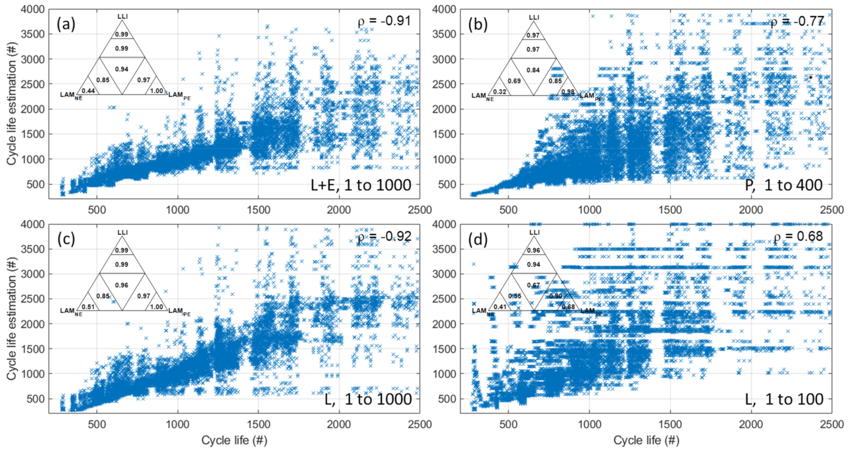
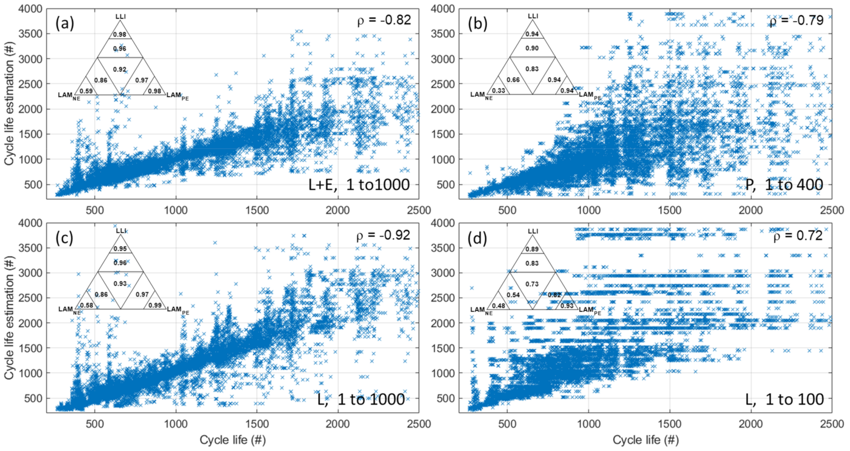
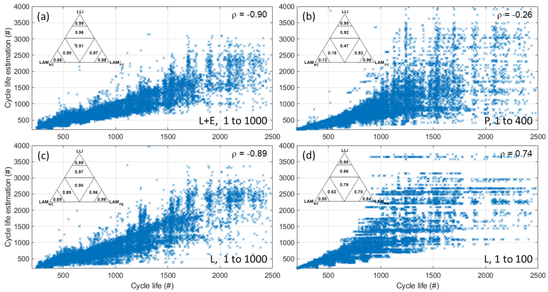
The trends observed from duty cycle #22050 are confirmed by the statistical study of the cycle life estimation obtained from the different fits over the entire duty cycle databases, Table 4. Figure 7 presents the relationship between the estimated end of life cycle (EOL) and the simulated one for the LFP cell and four different fits (L + E 1–1000, P 1–400, L 1–200, and L 1–100) with the impact of path dependency as inset. Similar data for the NCA and NMC cells are provided in Appendix B Figure A4 and Figure A8, respectively. Results are summarized in Table 4 where the early prognosis cycle life estimations are compared in terms of correlation coefficients, root-mean-square error (RMSE), mean absolute percentage error (MAPE), and coefficient of determination (R2). This is to compare the results with literature, notably [6,12] and [77]. As explained in [77], RMSE is more sensitive to large errors and describes the variations in data errors, MAPE measures the relative error and depicts the error in terms of percentages, and R2 represents better performance. Unsurprisingly, since equation A1 was the one used to simulate the duty cycles, the fit using the L + E function and cycles 1 to 1000 is showing high correlation with the simulated duty cycles for all three chemistries (ρ > 0.9, RMSE < 200 cycles, MAPE < 20%, R2 > 0.73) but the correlation goes down quickly for earlier prognosis, down to ρ < 0.45 with RMSE > 500 cycles, MAPE > 45%, and bad R2. The power fits perform slightly worse than the L + E fits with a maximum ρ of 0.85 and a minimum of 0.20. Looking at the linear fits, the performance is on par with the L + E fits for the 1 to 1000 range but better for the earlier prognosis with correlation coefficients around 0.7 for the cycles 1 to 100 fits, although the RMSE, MAPE, and R2 remained similar to the ones of the L + E fits.
Overall, the statistics reported in Table 4 might seem to be worse than the ones reported in the literature for an early prognosis at cycle 100 (RMSE ~100 cycles, MAPE ~ 10%, and R2 ~ 0.9) [6,12,77] but it must be reminded that the dataset used in these studies only covered a narrow set of experimental conditions and, therefore, cannot be compared to an early prognosis on the entire degradation spectrum. To enable a better comparison, the statistics were also computed for different paths of degradation. Results are reported in the insets of Figure 7, Figure A4, and Figure A8 but also in Table 5, Table A6 as well as Table A9 for LFO, NCA, and NMC, respectively, for cycles 1 to 200 and 1 to 100. The analysis shows that for paths with high LLI or high LAMPE, correlations coefficients above 0.9 are possible for early diagnosis at cycle 100 with RMSE below 100 cycles, MAPE below 10%, and R2 > 0.8, therefore, at levels comparable to the literature.
Based on our analysis, the early diagnosis based on a linear extrapolation of the diagnosed LLI and LAMs seems to offer interesting results for degradation paths containing mainly LLI or LAMPE. To be able to compare our early diagnosis methodology to the literature [6,12,77], the dataset on which the statistics are tabulated must be adapted. In the dataset provided in [6], the capacity loss is associated with LLI at a linear rate of about 0.005% per cycle. The acceleration of the degradation was associated with LAMNE. The fact that the acceleration is delayed for most cells suggests that LAMNE is just slightly higher than LLI. Moreover, since no evidence of peak ⓪ was reported, the lithium plating can be considered 100% irreversible. There was also no suggestion of any impact of the PE. In addition, the tested rate was 4C, far higher than our C/25. Unfortunately, our current definition of the duty cycles does not cover these conditions enough to offer significant statistics to compare. Further work is in progress to replicate the degradation observed in [6] with the synthetic datasets.
5. Conclusions
In this work, the strategy for the generation of synthetic datasets was refined to increase the resolution of the data to 1001 points for each voltage vs. capacity curve compared to 201 in the previous iteration, a fivefold increase. Moreover, changes in the duty cycle generation process allowed to reduce the size of the dataset by a factor of 200 if the diagnosis dataset is attached. This enables to increase the number of simulated duty cycles by two orders of magnitude without reaching the variable size limitation for MATLAB© on a normal laptop. In addition to improvements in the synthetic duty cycle generation and an update on the LFP dataset, we provided data for two other chemistries, NCA and NMC. These datasets provide the community with additional data to better validate diagnosis and prognosis tools on a wider array of possible degradations and they could be used as a Tier 1 challenge for deep and statistical learning early prognosis in the Battery Data Genome.
We also performed a statistical analysis of the datasets. Our investigation showcased that although a single FOI-based diagnosis is not effective, considering several FOIs together can offer accuracies below 1% up to cycle 400 for LLI, LAMPE, LAMNE, and capacity loss estimations. An extrapolation of this diagnosis allowed to prognose end-of-life with accuracies comparable with state-of-the-art for degradation paths with high LLI or LAMPE. It also showcased that the diagnosability and the prognosability are highly dependent on the degradation paths and that new methodologies must be validated on diverse datasets to be considered validated.
Author Contributions
Conceptualization, M.D.; methodology, M.D.; software, M.D.; validation, M.D. and D.B.; formal analysis, M.D. and D.B.; investigation, M.D.; resources, M.D.; data curation, M.D.; writing—original draft preparation, M.D.; writing—review and editing, M.D. and D.B.; visualization, M.D.; supervision, M.D.; project administration, M.D.; funding acquisition, M.D. All authors have read and agreed to the published version of the manuscript.
Funding
This research was funded by the Office of Naval Research, grant number N00014-18-1-2127 and N00014-19-1-2159.
Data Availability Statement
The data used in this study is available for download. LFP: http://dx.doi.org/10.17632/bs2j56pn7y.3 and http://dx.doi.org/10.17632/6s6ph9n8zg.3, NCA: http://dx.doi.org/10.17632/2h8cpszy26.1, NMC: http://dx.doi.org/10.17632/pb5xpv8z5r.1.
Conflicts of Interest
The authors declare no conflict of interest.
Appendix A. Simulation Parameters
Appendix A.1. Cell Emulation

Table A1.
Summary of alawa emulation parameters for the cells simulated in this work.
| Parameter | LFP | NCA | NMC811 |
|---|---|---|---|
| PE | ANR26650M [23,45] | NCR 18650B [35,40,41,42,43] | INR18650-35E [44] |
| NE | ANR26650M [23,45] | NCR 18650B [35,40,41,42,43] | Stock electrode |
| Loading ratio | 0.95 | 1.05 | 0.90 |
| Offset | 12.5 | 1.5 | 10 |
| Resistance adjustment | −0.07 | −0.18 | 0 |
| PE kinetic adjustment | None | None | None |
| NE kinetic adjustment | None | 0.75 | None |
Appendix A.2. Duty Cycle Calculations
As detailed in [26], a duty cycle is defined as the unique evolution of the triplet (LLI, LAMPE, LAMNE) with cycle number. In this work, the duty cycles are not associated with any particular charge or discharge cycle, nor a specific current, temperature, cutoff voltage, etc. Varying these conditions will change how the cell degrades, and per our definition of degradation, change the mix of LLI and LAMs the cell will experience. Since we are scanning all the possible LLI and LAMs combinations, our focus is set on how the cell is degraded independently of how it got there. The duty cycle dataset was calculated by varying eight parameters, Table A1. For all three degradation modes (LLI, LAMPE, and LAMNE, the degradation was chosen to follow Equation A1 where a and b corresponds to parameters p1 and p2 for LLI, p3, and p4 for LAMPE, and p5 and p6 for LAMNE. Parameter p7 addresses a delay for the exponential response for LLI.
The plating threshold (PT) [26,35] at which lithium plating starts to happen was calculated using Equation (A2). Parameter p8 addresses the reversibility of lithium plating following Equation (A3).
Fitting equations:
Table A2.
Summary of scanned parameters for the duty cycle dataset.
| Parameter | Description | Values (% per Cycle) |
|---|---|---|
| p1 | Linear Coeff. LLI | 0.007, 0.010, 0.013, 0.017, 0.021, 0.027, 0.034, 0.048, 0.06 |
| p2 | Exp. Coeff. LLI | 0.000001, 0.002, 0.0033 |
| p3 | Delay Exp. LLI | 600, 1200, 1800 |
| p4 | Linear Coeff. LAMPE | 0.001, 0.005, 0.01, 0.015, 0.02, 0.025, 0.03, 0.0375, 0.05, 0.07 |
| p5 | Exp. Coeff. LAMPE | 0.000001, 0.001, 0.0013 |
| p6 | Linear Coeff. LAMNE | 0.001, 0.005, 0.0,1 0.015, 0.02, 0.025, 0.03, 0.0375, 0.05, 0.07 |
| p7 | Exp. Coeff. LAMNE | 0.000001, 0.001, 0.0013 |
| p8 | Plating Reversibility | 0, 50, 100 |
Appendix A.3. FOI Selection and Resolution
Table A3.
Summary of selected FOIs with resolution in palapala‘aina [24] 3D maps.
Table A3.
Summary of selected FOIs with resolution in palapala‘aina [24] 3D maps.
| FOI | Description | Resolution in 3D Map |
|---|---|---|
| LFP-FOI1 | Area between 3.35 and 3.40 V | 0.4% Q |
| LFP-FOI2 | Area between 3.20 and 3.35 V | 0.6% Q |
| LFP-FOI3 | Position maximum between 3.00 and 3.25 V | 0.002 V |
| LFP-FOI4 | Intensity maximum between 3.00 and 3.25 V | 3.5% Q/V |
| LFP-FOI5 | Area between 3.42 and 3.50 V | 1.0% Q |
| NCA-FOI1 | Area between 4.02 and 4.05 V | 0.04%Q |
| NCA-FOI2 | Position minimum between 3.60 and 3.98 V | 0.004 V |
| NCA-FOI3 | Intensity minimum between 3.60 and 3.98 V | 1.2% Q/V |
| NCA-FOI4 | Capacity difference between 2 peaks between 20 and 60% Q | 0.4% Q |
| NCA-FOI5 | Area between 4.15 and 4.255 V | 0.1% Q |
| NCA-FOI6 | Intensity maximum between 3.00 and 3.6 V | 6% Q/V |
| NCA-FOI7 | Position maximum between 3.00 and 3.6 V | 0.006 V |
| NMC-FOI1 | Area between 4.02 and 4.05 V | 0.04% Q |
| NMC-FOI2 | Position minimum between 3.60 and 3.98 V | 0.004 V |
| NMC-FOI3 | Intensity minimum between 3.60 and 3.98 V | 1% Q/V |
| NMC-FOI4 | Capacity difference between 2 peaks between 20 and 60% Q | 0.4% Q |
| NMC-FOI5 | Area between 4.15 and 4.295 V | 0.18 % Q |
| NMC-FOI6 | Intensity maximum between 3.00 and 3.59 V | 3% Q/V |
| NMC-FOI7 | Position maximum between 3.00 and 3.59 V | 0.006 V |
Appendix B. Supplementary Tables and Figures
Appendix B.1. Gr//NCA, C/33 Charge
Table A4.
Correlation table for the NCA cell at cycle 100. Light gray indicates |ρ| > 0.5 and dark gray |ρ| > 0.8.
Table A4.
Correlation table for the NCA cell at cycle 100. Light gray indicates |ρ| > 0.5 and dark gray |ρ| > 0.8.
| LLI | LAMPE | LAMNE | Capacity Loss | |
|---|---|---|---|---|
| FOI1 | 0.08 | −0.98 | −0.08 | −0.44 |
| FOI2 | 0.73 | −0.46 | −0.41 | 0.24 |
| FOI3 | −0.89 | 0.18 | 0.11 | −0.48 |
| FOI4 | 0.08 | −0.51 | −0.64 | −0.50 |
| FOI5 | −0.35 | −0.65 | 0.64 | −0.49 |
| FOI6 | −0.63 | 0.53 | −0.24 | −0.40 |
| FOI7 | 0.68 | −0.66 | 0.18 | 0.27 |
| FOIs (1,2,4) | 0.95 | 0.96 | 0.89 | 0.97 |
| FOIs (1,3,4) | 0.85 | 0.96 | 0.92 | 0.82 |
| FOIs (1,5,4) | 0.74 | 0.98 | 0.89 | 0.88 |
| FOIs (1,6,4) | 0.89 | 0.95 | 0.89 | 0.93 |
| FOIs (1,7,4) | 0.83 | 0.96 | 0.90 | 0.88 |
Table A5.
Mean estimation errors for the NCA cell (from FOIs 1, 2, and 4).
| LLI | LAMPE | LAMNE | Capacity Loss | |||||||||
|---|---|---|---|---|---|---|---|---|---|---|---|---|
| Cycle 10 | 0.07 | ± | 0.16 | 0.07 | ± | 0.17 | −0.01 | ± | 0.20 | 0.06 | ± | 0.15 |
| Cycle 50 | −0.11 | ± | 0.27 | −0.12 | ± | 0.43 | −0.15 | ± | 0.41 | −0.11 | ± | 0.30 |
| Cycle 100 | −0.10 | ± | 0.42 | −0.02 | ± | 0.50 | −0.18 | ± | 0.83 | −0.01 | ± | 0.35 |
| Cycle 200 | −0.14 | ± | 0.95 | 0.13 | ± | 0.97 | −0.16 | ± | 2.30 | 0.14 | ± | 0.76 |
| Cycle 400 | −0.09 | ± | 2.28 | 0.29 | ± | 2.57 | −0.17 | ± | 4.37 | 0.42 | ± | 2.39 |
| Cycle 1000 | −0.67 | ± | 7.22 | −0.02 | ± | 5.21 | −2.64 | ± | 9.02 | 0.08 | ± | 4.96 |
Table A6.
Correlation table for the early prognosis established from the linear diagnosis.
| Linear Fit, Cycles 1–200 | Linear Fit, Cycles 1–100 | ||||||||
|---|---|---|---|---|---|---|---|---|---|
| ρ | RMSE | MAPE | R2 | ρ | RMSE | MAPE | R2 | ||
| >50% LLI | 0.96 | 191 | 6 | 0.75 | 0.83 | 403 | 15 | −0.12 | |
| >80% LLI | 0.97 | 87 | 3 | 0.94 | 0.89 | 273 | 8 | 0.38 | |
| >50% LAMPE | 0.96 | 102 | 7 | 0.78 | 0.82 | 321 | 11 | −1.24 | |
| >80% LAMPE | 0.98 | 32 | 5 | 0.92 | 0.93 | 71 | 7 | 0.63 | |
| >50% LAMNE | 0.65 | 616 | 43 | −1.41 | 0.54 | 968 | 69 | −4.95 | |
| >80% LAMNE | 0.60 | 487 | 22 | −0.34 | 0.48 | 1059 | 38 | −5.34 | |
| <50% all | 0.86 | 335 | 17 | −0.12 | 0.73 | 591 | 38 | −2.48 | |
Figure A1.
Correlation between the most adapted FOI and the percentage of (a) LLI, (b) LAMPE, (c) LAMNE, and (d) the capacity loss for the NCA C/33 charges at cycle 100.
Figure A1.
Correlation between the most adapted FOI and the percentage of (a) LLI, (b) LAMPE, (c) LAMNE, and (d) the capacity loss for the NCA C/33 charges at cycle 100.

Figure A2.
Mean diagnosis errors for the >125,000 duty cycle as a function of cycle number for (a) LLI, (b) LAMPE, (c) LAMNE, and (d) the capacity loss for the NCA C/33 charges. Inset ternary diagrams represent the standard deviation between the diagnosis and the real value for different degradation paths at cycles 100 and 400.

Figure A3.
Evolution of (a) the variance between cycle 100 and 1 for NCA C/33 charges, (b) the variance between cycles 400 and 1, (c) the capacity loss at cycle 100, and (d) the area of the high voltage IC peak at cycle 100 as a function of cycle life (i.e., cycle at which 20% capacity loss is reached). Insert presents correlation as a function of degradation mix.

Figure A4.
Predicted vs. simulated EOL cycle correlation for (a) a linear and exponential fit of the diagnosis for cycles 1 to 1000, (b) a power fit of the diagnosis for cycles 1 to 400, (c) a linear fit of the diagnosis for cycles 1 to 200, and (d) a linear fit of the diagnosis for cycles 1 to 100. Insert presents correlation as a function of degradation mix.

Appendix B.2. GIC//NMC811 C/25 Charges
Table A7.
Correlation table for the NMC811 cell at cycle 100. Light gray indicates |ρ| > 0.5 and dark gray |ρ| > 0.8.
Table A7.
Correlation table for the NMC811 cell at cycle 100. Light gray indicates |ρ| > 0.5 and dark gray |ρ| > 0.8.
| LLI | LAMPE | LAMNE | Capacity Loss | |
|---|---|---|---|---|
| FOI1 | 0.10 | −0.95 | −0.08 | 0.05 |
| FOI2 | 0.51 | −0.24 | −0.04 | 0.45 |
| FOI3 | 0.63 | −0.65 | 0.08 | 0.57 |
| FOI4 | −0.46 | 0.03 | −0.96 | −0.57 |
| FOI5 | −0.09 | −0.89 | 0.36 | −0.06 |
| FOI6 | 0.41 | −0.18 | −0.13 | 0.35 |
| FOI7 | 0.42 | −0.41 | 0.44 | 0.45 |
| FOIs (1,2,4) | 0.98 | 0.94 | 0.94 | 0.98 |
| FOIs (1,3,4) | 0.89 | 0.92 | 0.94 | 0.90 |
| FOIs (1,5,4) | 0.65 | 0.96 | 0.94 | 0.69 |
| FOIs (1,6,4) | 0.70 | 0.92 | 0.94 | 0.72 |
| FOIs (1,7,4) | 0.94 | 0.93 | 0.94 | 0.95 |
Table A8.
Mean estimation errors for the NMC811 cell (from FOIs 1, 2, and 4).
| LLI | LAMPE | LAMNE | Capacity Loss | |||||||||
|---|---|---|---|---|---|---|---|---|---|---|---|---|
| Cycle 10 | 0.11 | ± | 0.20 | 0.15 | ± | 0.19 | 0.08 | ± | 0.22 | 0.12 | ± | 0.22 |
| Cycle 50 | −0.11 | ± | 0.31 | −0.14 | ± | 0.53 | −0.11 | ± | 0.52 | −0.12 | ± | 0.36 |
| Cycle 100 | −0.08 | ± | 0.32 | −0.08 | ± | 0.57 | −0.09 | ± | 0.59 | −0.08 | ± | 0.38 |
| Cycle 200 | 0.16 | ± | 1.37 | 0.14 | ± | 1.52 | 0.17 | ± | 1.82 | 0.27 | ± | 1.85 |
| Cycle 400 | 0.45 | ± | 3.14 | 0.67 | ± | 3.73 | 0.91 | ± | 4.56 | 0.99 | ± | 4.07 |
| Cycle 1000 | −0.62 | ± | 5.58 | 0.23 | ± | 5.34 | −0.59 | ± | 8.48 | 0.28 | ± | 5.06 |
Table A9.
Correlation table for the early prognosis established from the linear diagnosis.
| Linear Fit, Cycles 1–200 | Linear Fit, Cycles 1–100 | |||||||
|---|---|---|---|---|---|---|---|---|
| ρ | RMSE | MAPE | R2 | ρ | RMSE | MAPE | R2 | |
| >50% LLI | 0.97 | 117 | 7 | 0.87 | 0.96 | 131 | 8 | 0.84 |
| >80% LLI | 0.98 | 101 | 4 | 0.90 | 0.95 | 150 | 7 | 0.78 |
| >50% LAMPE | 0.83 | 277 | 33 | 0.01 | 0.70 | 517 | 34 | −2.45 |
| >80% LAMPE | 0.96 | 217 | 36 | −0.64 | 0.84 | 193 | 30 | −0.30 |
| >50% LAMNE | 0.86 | 308 | 14 | 0.55 | 0.62 | 786 | 22 | −1.92 |
| >80% LAMNE | 0.55 | 508 | 20 | −0.38 | 0.50 | 530 | 23 | −0.50 |
| <50% all | 0.86 | 238 | 13 | 0.47 | 0.79 | 484 | 21 | −1.18 |
Figure A5.
Correlation between the most adapted FOI and the percentage of (a) LLI, (b) LAMPE, (c) LAMNE, and (d) the capacity loss for the NMC811 C/25 charges at cycle 100.
Figure A5.
Correlation between the most adapted FOI and the percentage of (a) LLI, (b) LAMPE, (c) LAMNE, and (d) the capacity loss for the NMC811 C/25 charges at cycle 100.

Figure A6.
Mean diagnosis errors for the >125,000 duty cycle as a function of cycle number for (a) LLI, (b) LAMPE, (c) LAMNE, and (d) the capacity loss for the NMC811 C/25 charges. Inset ternary diagrams represent the correlation between the diagnosis and the real value for different degradation paths at cycles 100 and 400.

Figure A7.
Evolution of (a) the variance between cycle 100 and 1 for NMC811 C/25 charges, (b) the variance between cycles 400 and 1, (c) the capacity loss at cycle 100, and (d) the area of the high voltage IC peak at cycle 100 as a function of cycle life (i.e., cycle at which 20% capacity loss is reached). Insert presents correlation as a function of degradation mix.

Figure A8.
Predicted vs. simulated EOL cycle correlation for (a) a linear and exponential fit of the diagnosis for cycles 1 to 1000, (b) a power fit of the diagnosis for cycles 1 to 400, (c) a linear fit of the diagnosis for cycles 1 to 200, and (d) a linear fit of the diagnosis for cycles 1 to 100. Insert presents correlation as a function of degradation mix.

References
- Raj, T.; Wang, A.A.; Monroe, C.W.; Howey, D.A. Investigation of Path-Dependent Degradation in Lithium-Ion Batteries. Batter. Supercaps 2020, 3, 1377–1385. [Google Scholar] [CrossRef]
- Gering, K.L.; Sazhin, S.V.; Jamison, D.K.; Michelbacher, C.J.; Liaw, B.Y.; Dubarry, M.; Cugnet, M. Investigation of path dependence in commercial lithium-ion cells chosen for plug-in hybrid vehicle duty cycle protocols. J. Power Sources 2011, 196, 3395–3403. [Google Scholar] [CrossRef]
- Ng, M.-F.; Zhao, J.; Yan, Q.; Conduit, G.J.; Seh, Z.W. Predicting the state of charge and health of batteries using data-driven machine learning. Nat. Mach. Intell. 2020, 2, 161–170. [Google Scholar] [CrossRef] [Green Version]
- Vidal, C.; Malysz, P.; Kollmeyer, P.; Emadi, A. Machine Learning Applied to Electrified Vehicle Battery State of Charge and State of Health Estimation: State-of-the-Art. IEEE Access 2020, 8, 52796–52814. [Google Scholar] [CrossRef]
- How, D.N.T.; Hannan, M.A.; Lipu, M.S.H.; Ker, P.J. State of Charge Estimation for Lithium-Ion Batteries Using Model-Based and Data-Driven Methods: A Review. IEEE Access 2019, 7, 136116–136136. [Google Scholar] [CrossRef]
- Severson, K.A.; Attia, P.M.; Jin, N.; Perkins, N.; Jiang, B.; Yang, Z.; Chen, M.H.; Aykol, M.; Herring, P.K.; Fraggedakis, D.; et al. Data-driven prediction of battery cycle life before capacity degradation. Nat. Energy 2019, 4, 383–391. [Google Scholar] [CrossRef] [Green Version]
- Klass, V.; Behm, M.; Lindbergh, G. A support vector machine-based state-of-health estimation method for lithium-ion batteries under electric vehicle operation. J. Power Sources 2014, 270, 262–272. [Google Scholar] [CrossRef]
- Klass, V.; Behm, M.; Lindbergh, G. Evaluating Real-Life Performance of Lithium-Ion Battery Packs in Electric Vehicles. J. Electrochem. Soc. 2012, 159, A1856–A1860. [Google Scholar] [CrossRef]
- Hu, C.; Jain, G.; Schmidt, C.L.; Strief, C.; Sullivan, M. Online estimation of lithium-ion battery capacity using sparse Bayesian learning. J. Power Sources 2015, 289, 105–113. [Google Scholar] [CrossRef]
- Richardson, R.R.; Birkl, C.R.; Osborne, M.A.; Howey, D.A. Gaussian Process Regression for In Situ Capacity Estimation of Lithium-Ion Batteries. IEEE Trans. Ind. Inform. 2019, 15, 127–138. [Google Scholar] [CrossRef] [Green Version]
- Pan, H.; Lü, Z.; Wang, H.; Wei, H.; Chen, L. Novel battery state-of-health online estimation method using multiple health indicators and an extreme learning machine. Energy 2018, 160, 466–477. [Google Scholar] [CrossRef]
- Attia, P.M.; Grover, A.; Jin, N.; Severson, K.A.; Markov, T.M.; Liao, Y.-H.; Chen, M.H.; Cheong, B.; Perkins, N.; Yang, Z.; et al. Closed-loop optimization of fast-charging protocols for batteries with machine learning. Nat. Cell Biol. 2020, 578, 397–402. [Google Scholar] [CrossRef] [Green Version]
- Cripps, E.; Pecht, M. A Bayesian nonlinear random effects model for identification of defective batteries from lot samples. J. Power Sources 2017, 342, 342–350. [Google Scholar] [CrossRef]
- Roman, D.; Saxena, S.; Robu, V.; Pecht, M.; Flynn, D. Machine learning pipeline for battery state-of-health estimation. Nat. Mach. Intell. 2021, 1–10. [Google Scholar] [CrossRef]
- Attia, P.M.; Severson, K.A.; Witmer, J.D. Statistical learning for accurate and interpretable battery lifetime prediction. arXiv 2021, arXiv:2101.01885. [Google Scholar]
- Kollmeyer, P.; Vidal, C.; Naguib, M.; Skells, M. LG 18650HG2 Li-ion Battery Data and Example Deep Neural Network xEV SOC Estimator Script. Available online: https://data.mendeley.com/datasets/cp3473x7xv/3 (accessed on 12 April 2021).
- Kollmeyer, P. Panasonic 18650PF Li-ion Battery Data, Mendeley Data, v1. Available online: https://data.mendeley.com/datasets/wykht8y7tg/1#folder96f196a8-a04d-4e6a-827d-0dc4d61ca97b (accessed on 12 April 2021).
- Saha, B.; Goebel, K. Battery Data Set. In NASA Ames Prognostics Data Repository; NASA Ames Research Center: Moffett Field, CA, USA. Available online: https://ti.arc.nasa.gov/tech/dash/groups/pcoe/prognostic-data-repository/ (accessed on 12 April 2021).
- Barkholtz, H.M.; Fresquez, A.; Chalamala, B.R.; Ferreira, S.R. A Database for Comparative Electrochemical Performance of Commercial 18650-Format Lithium-Ion Cells. J. Electrochem. Soc. 2017, 164, A2697–A2706. [Google Scholar] [CrossRef]
- Pecht, M. Battery Research Data. Available online: https://calce.umd.edu/data (accessed on 12 April 2021).
- Birkl, C.R.; Offer, G.J. Oxford Battery Degradation Dataset from the Howey Research Group. Available online: https://ora.ox.ac.uk/objects/uuid%3a03ba4b01-cfed-46d3-9b1a-7d4a7bdf6fac (accessed on 14 April 2021).
- Aykol, M.; Babinec, S.; Beck, D.A.C.; Blaiszik, B.; Chen, B.R.; Crabtree, G.; Angelis, V.D.; Dechent, P.; Dubarry, M.; Dufek, E.; et al. Principles of a Battery Data Genome. Nature 2021. under review. [Google Scholar]
- Anseán, D.; Dubarry, M.; Devie, A.; Liaw, B.; García, V.; Viera, J.; González, M. Operando lithium plating quantification and early detection of a commercial LiFePO4 cell cycled under dynamic driving schedule. J. Power Sources 2017, 356, 36–46. [Google Scholar] [CrossRef] [Green Version]
- Dubarry, M.; Berecibar, M.; Devie, A.; Anseán, D.; Omar, N.; Villarreal, I. State of health battery estimator enabling degradation diagnosis: Model and algorithm description. J. Power Sources 2017, 360, 59–69. [Google Scholar] [CrossRef]
- Dubarry, M.; Baure, G.; Anseán, D. Perspective on State-of-Health Determination in Lithium-Ion Batteries. J. Electrochem. Energy Convers. Storage 2020, 17, 1–25. [Google Scholar] [CrossRef]
- Dubarry, M.; Beck, D. Big data training data for artificial intelligence-based Li-ion diagnosis and prognosis. J. Power Sources 2020, 479, 228806. [Google Scholar] [CrossRef]
- Bloom, I.; Jansen, A.N.; Abraham, D.P.; Knuth, J.; Jones, S.A.; Battaglia, V.S.; Henriksen, G.L. Differential voltage analyses of high-power, lithium-ion cells. J. Power Sources 2005, 139, 295–303. [Google Scholar] [CrossRef]
- Honkura, K.; Honbo, H.; Koishikawa, Y.; Horiba, T. State Analysis of Lithium-Ion Batteries Using Discharge Curves. ECS Meet. Abstr. 2008, 13, 61–73. [Google Scholar] [CrossRef]
- Dahn, H.M.; Smith, A.J.; Burns, J.C.; Stevens, D.A.; Dahn, J.R. User-Friendly Differential Voltage Analysis Freeware for the Analysis of Degradation Mechanisms in Li-Ion Batteries. J. Electrochem. Soc. 2012, 159, A1405–A1409. [Google Scholar] [CrossRef]
- Dubarry, M.; Truchot, C.; Liaw, B.Y. Synthesize battery degradation modes via a diagnostic and prognostic model. J. Power Sources 2012, 219, 204–216. [Google Scholar] [CrossRef]
- Dubarry, M. Graphite//LFP synthetic training duty cycle dataset. Mendeley Data. 2020, Volume 2021. Available online: https://data.mendeley.com/datasets/6s6ph9n8zg/1 (accessed on 14 April 2021).
- Dubarry, M. Graphite//LFP synthetic training V vs. Q dataset. Mendeley Data. 2020, Volume 2021. Available online: https://data.mendeley.com/datasets/6s6ph9n8zg/2 (accessed on 14 April 2021).
- Dubarry, M. Graphite//NCA synthetic V vs. Q & duty cycle datasets. Mendeley Data. 2021. Available online: https://data.mendeley.com/datasets/2h8cpszy26/1 (accessed on 14 April 2021).
- Dubarry, M. Graphite//NMC synthetic V vs. Q & duty cycle datasets. Mendeley Data. 2021. Available online: https://data.mendeley.com/datasets/pb5xpv8z5r/1 (accessed on 14 April 2021).
- Baure, G.; Dubarry, M. Synthetic vs. Real Driving Cycles: A Comparison of Electric Vehicle Battery Degradation. Batteries 2019, 5, 42. [Google Scholar] [CrossRef] [Green Version]
- Gao, Y.; Yang, S.; Jiang, J.; Zhang, C.; Zhang, W.; Zhou, X. The Mechanism and Characterization of Accelerated Capacity Deterioration for Lithium-Ion Battery with Li(NiMnCo) O2 Cathode. J. Electrochem. Soc. 2019, 166, A1623–A1635. [Google Scholar] [CrossRef]
- Yang, X.-G.; Leng, Y.; Zhang, G.; Ge, S.; Wang, C.-Y. Modeling of lithium plating induced aging of lithium-ion batteries: Transition from linear to nonlinear aging. J. Power Sources 2017, 360, 28–40. [Google Scholar] [CrossRef]
- Schuster, S.F.; Bach, T.; Fleder, E.; Müller, J.; Brand, M.; Sextl, G.; Jossen, A. Nonlinear aging characteristics of lithium-ion cells under different operational conditions. J. Energy Storage 2015, 1, 44–53. [Google Scholar] [CrossRef]
- Keil, P.; Jossen, A. Charging protocols for lithium-ion batteries and their impact on cycle life—An experimental study with different 18650 high-power cells. J. Energy Storage 2016, 6, 125–141. [Google Scholar] [CrossRef]
- Devie, A.; Dubarry, M. Durability and Reliability of Electric Vehicle Batteries under Electric Utility Grid Operations. Part 1: Cell-to-Cell Variations and Preliminary Testing. Batteries 2016, 2, 28. [Google Scholar] [CrossRef]
- Dubarry, M.; Baure, G.; Devie, A. Durability and Reliability of EV Batteries under Electric Utility Grid Operations: Path Dependence of Battery Degradation. J. Electrochem. Soc. 2018, 165, A773–A783. [Google Scholar] [CrossRef]
- Dubarry, M.; Devie, A.; McKenzie, K. Durability and reliability of electric vehicle batteries under electric utility grid operations: Bidirectional charging impact analysis. J. Power Sources 2017, 358, 39–49. [Google Scholar] [CrossRef]
- Schindler, S.; Baure, G.; Danzer, M.A.; Dubarry, M. Kinetics accommodation in Li-ion mechanistic modeling. J. Power Sources 2019, 440, 227117. [Google Scholar] [CrossRef]
- Anseán, D.; Baure, G.; González, M.; Cameán, I.; García, A.; Dubarry, M. Mechanistic investigation of silicon-graphite/LiNi0.8Mn0.1Co0.1O2 commercial cells for non-intrusive diagnosis and prognosis. J. Power Sources 2020, 459, 227882. [Google Scholar] [CrossRef]
- Anseán, D.; Dubarry, M.; Devie, A.; Liaw, B.; García, V.; Viera, J.; González, M. Fast charging technique for high power LiFePO4 batteries: A mechanistic analysis of aging. J. Power Sources 2016, 321, 201–209. [Google Scholar] [CrossRef]
- Dubarry, M.; Baure, G. Perspective on Commercial Li-ion Battery Testing, Best Practices for Simple and Effective Protocols. Electron. 2020, 9, 152. [Google Scholar] [CrossRef] [Green Version]
- Fath, J.P.; Dragicevic, D.; Bittel, L.; Nuhic, A.; Sieg, J.; Hahn, S.; Alsheimer, L.; Spier, B.; Wetzel, T. Quantification of aging mechanisms and inhomogeneity in cycled lithium-ion cells by differential voltage analysis. J. Energy Storage 2019, 25. [Google Scholar] [CrossRef]
- Nuhic, A.; Terzimehic, T.; Soczka-Guth, T.; Buchholz, M.; Dietmayer, K. Health diagnosis and remaining useful life prognostics of lithium-ion batteries using data-driven methods. J. Power Sources 2013, 239, 680–688. [Google Scholar] [CrossRef]
- Liu, D.; Luo, Y.; Liu, J.; Peng, Y.; Guo, L.; Pecht, M. Lithium-ion battery remaining useful life estimation based on fusion nonlinear degradation AR model and RPF algorithm. Neural Comput. Appl. 2013, 25, 557–572. [Google Scholar] [CrossRef]
- Liu, D.; Pang, J.; Zhou, J.; Peng, Y.; Pecht, M. Prognostics for state of health estimation of lithium-ion batteries based on combination Gaussian process functional regression. Microelectron. Reliab. 2013, 53, 832–839. [Google Scholar] [CrossRef]
- Lee, C.; Jo, S.; Kwon, D.; Pecht, M.G. Capacity-Fading Behavior Analysis for Early Detection of Unhealthy Li-Ion Batteries. IEEE Trans. Ind. Electron. 2021, 68, 2659–2666. [Google Scholar] [CrossRef]
- Strange, C.; Li, S.; Gilchrist, R.; dos Reis, G. Elbows of Internal Resistance Rise Curves in Li-Ion Cells. Energies 2021, 14, 1206. [Google Scholar] [CrossRef]
- Lee, J.; Kwon, D.; Pecht, M.G. Reduction of Li-ion Battery Qualification Time Based on Prognostics and Health Management. IEEE Trans. Ind. Electron. 2018, 66, 7310–7315. [Google Scholar] [CrossRef]
- Fermín-Cueto, P.; McTurk, E.; Allerhand, M.; Medina-Lopez, E.; Anjos, M.F.; Sylvester, J.; dos Reis, G. Identification and machine learning prediction of knee-point and knee-onset in capacity degradation curves of lithium-ion cells. Energy AI 2020, 1, 100006. [Google Scholar] [CrossRef]
- Yang, D.; Zhang, X.; Pan, R.; Wang, Y.; Chen, Z. A novel Gaussian process regression model for state-of-health estimation of lithium-ion battery using charging curve. J. Power Sources 2018, 384, 387–395. [Google Scholar] [CrossRef]
- Goh, T.; Park, M.; Seo, M.; Kim, J.G.; Kim, S.W. Successive-approximation algorithm for estimating capacity of Li-ion batteries. Energy 2018, 159, 61–73. [Google Scholar] [CrossRef]
- Goh, T.; Park, M.; Seo, M.; Kim, J.G.; Kim, S.W. Capacity estimation algorithm with a second-order differential voltage curve for Li-ion batteries with NMC cathodes. Energy 2017, 135, 257–268. [Google Scholar] [CrossRef]
- Eddahech, A.; Briat, O.; Bertrand, N.; Delétage, J.-Y.; Vinassa, J.-M. Behavior and state-of-health monitoring of Li-ion batteries using impedance spectroscopy and recurrent neural networks. Int. J. Electr. Power Energy Syst. 2012, 42, 487–494. [Google Scholar] [CrossRef]
- Saha, B.; Poll, S.; Goebel, K.; Christophersen, J. An Integrated Approach to Battery Health Monitoring Using Bayesian Regression and State Estimation; International Automatic Testing Conference: Baltimore, MD, USA, 2007; pp. 646–653. [Google Scholar]
- Zhang, Y.; Tang, Q.; Zhang, Y.; Wang, J.; Stimming, U.; Lee, A.A. Identifying degradation patterns of lithium ion batteries from impedance spectroscopy using machine learning. Nat. Commun. 2020, 11, 216. [Google Scholar] [CrossRef]
- Marongiu, A.; Nlandi, N.; Rong, Y.; Sauer, D.U. On-board capacity estimation of lithium iron phosphate batteries by means of half-cell curves. J. Power Sources 2016, 324, 158–169. [Google Scholar] [CrossRef]
- Weng, C.; Cui, Y.; Sun, J.; Peng, H. On-board state of health monitoring of lithium-ion batteries using incremental capacity analysis with support vector regression. J. Power Sources 2013, 235, 36–44. [Google Scholar] [CrossRef]
- Tang, X.; Zou, C.; Yao, K.; Chen, G.; Liu, B.; He, Z.; Gao, F. A fast estimation algorithm for lithium-ion battery state of health. J. Power Sources 2018, 396, 453–458. [Google Scholar] [CrossRef]
- Li, Y.; Abdel-Monem, M.; Gopalakrishnan, R.; Berecibar, M.; Nanini-Maury, E.; Omar, N.; Bossche, P.V.D.; Van Mierlo, J. A quick on-line state of health estimation method for Li-ion battery with incremental capacity curves processed by Gaussian filter. J. Power Sources 2018, 373, 40–53. [Google Scholar] [CrossRef]
- Wang, L.; Zhao, X.; Liu, L.; Pan, C. State of health estimation of battery modules via differential voltage analysis with local data symmetry method. Electrochim. Acta 2017, 256, 81–89. [Google Scholar] [CrossRef]
- Berecibar, M.; Garmendia, M.; Gandiaga, I.; Crego, J.; Villarreal, I. State of health estimation algorithm of LiFePO4 battery packs based on differential voltage curves for battery management system application. Energy 2016, 103, 784–796. [Google Scholar] [CrossRef]
- Wang, L.; Pan, C.; Liu, L.; Cheng, Y.; Zhao, X. On-board state of health estimation of LiFePO4 battery pack through differential voltage analysis. Appl. Energy 2016, 168, 465–472. [Google Scholar] [CrossRef]
- Li, X.; Wang, Z.; Yan, J. Prognostic health condition for lithium battery using the partial incremental capacity and Gaussian process regression. J. Power Sources 2019, 421, 56–67. [Google Scholar] [CrossRef]
- Li, Y.; Liu, K.; Foley, A.M.; Zülke, A.; Berecibar, M.; Nanini-Maury, E.; Van Mierlo, J.; Hoster, H.E. Data-driven health estimation and lifetime prediction of lithium-ion batteries: A review. Renew. Sustain. Energy Rev. 2019, 113. [Google Scholar] [CrossRef]
- She, C.; Wang, Z.; Sun, F.; Liu, P.; Zhang, L. Battery Aging Assessment for Real-World Electric Buses Based on Incremental Capacity Analysis and Radial Basis Function Neural Network. IEEE Trans. Ind. Inform. 2020, 16, 3345–3354. [Google Scholar] [CrossRef]
- Sarasketa-Zabala, E.; Martinez-Laserna, E.; Berecibar, M.; Gandiaga, I.; Rodriguez-Martinez, L.; Villarreal, I. Realistic lifetime prediction approach for Li-ion batteries. Appl. Energy 2016, 162, 839–852. [Google Scholar] [CrossRef]
- Berecibar, M.; Devriendt, F.; Dubarry, M.; Villarreal, I.; Omar, N.; Verbeke, W.; Van Mierlo, J. Online state of health estimation on NMC cells based on predictive analytics. J. Power Sources 2016, 320, 239–250. [Google Scholar] [CrossRef]
- Harris, S.J.; Harris, D.J.; Li, C. Failure statistics for commercial lithium ion batteries: A study of 24 pouch cells. J. Power Sources 2017, 342, 589–597. [Google Scholar] [CrossRef] [Green Version]
- Sulzer, V.; Mohtat, P.; Lee, S.; Siegel, J.B.; Stefanopoulou, A.G. Promise and Challenges of a Data-Driven Approach for Battery Lifetime Prognostics. arXiv 2021, arXiv:2010.07460v1. [Google Scholar]
- Baure, G.; Dubarry, M. Battery durability and reliability under electric utility grid operations: 20-year forecast under different grid applications. J. Energy Storage 2020, 29, 101391. [Google Scholar] [CrossRef]
- Baure, G.; Devie, A.; Dubarry, M. Battery Durability and Reliability under Electric Utility Grid Operations: Path Dependence of Battery Degradation. J. Electrochem. Soc. 2019, 166, A1991–A2001. [Google Scholar] [CrossRef]
- Fei, Z.; Yang, F.; Tsui, K.-L.; Li, L.; Zhang, Z. Early prediction of battery lifetime via a machine learning based framework. Energy 2021, 225, 120205. [Google Scholar] [CrossRef]
Figure 1.
LFP, NCA, and NMC811 incremental capacity and differential voltage curves for the pristine and aged cell with 18% LAMNE with detail on the selected features of interest (FOI).
Figure 1.
LFP, NCA, and NMC811 incremental capacity and differential voltage curves for the pristine and aged cell with 18% LAMNE with detail on the selected features of interest (FOI).

Figure 2.
Example of duty cycle #22050 for the Gr//LFP cell with (a) the evolution of capacity loss, LLI, LAMPE, and LAMNE, (b) the associated incremental capacity curves, and (c) the evolution of the 5 FOIs selected for the Gr//LFP cell.
Figure 2.
Example of duty cycle #22050 for the Gr//LFP cell with (a) the evolution of capacity loss, LLI, LAMPE, and LAMNE, (b) the associated incremental capacity curves, and (c) the evolution of the 5 FOIs selected for the Gr//LFP cell.

Figure 3.
Correlation between the most adapted FOI and the percentage of (a) LLI, (b) LAMPE, (c) LAMNE, and (d) the capacity loss for the Gr//LFP cell at cycle 100. Each point corresponds to one duty cycle at cycle 100.
Figure 3.
Correlation between the most adapted FOI and the percentage of (a) LLI, (b) LAMPE, (c) LAMNE, and (d) the capacity loss for the Gr//LFP cell at cycle 100. Each point corresponds to one duty cycle at cycle 100.

Figure 4.
Mean diagnosis errors for the >125,000 duty cycle as a function of cycle number for (a) LLI, (b) LAMPE, (c) LAMNE, and (d) the capacity loss for the Gr//LFP cell. Inset ternary diagrams represent the standard deviation between the diagnosis and the real value for different degradation paths at cycles 100 and 400.

Figure 5.
Evolution of (a) the variance of voltage between cycles 100 and 1 for the LFP cell, (b) the voltage variance between cycles 400 and 1, (c) the capacity loss at cycle 100, and (d) the area of the IC peak ① at cycle 100 as a function of cycle life. Inset presents correlation as a function of degradation mix. End-of-life is defined as 20% capacity loss.

Figure 6.
Fits for duty cycle 22050 from diagnosis with (a) the linear + exponential, (b) the power, and (c) the linear fits.
Figure 6.
Fits for duty cycle 22050 from diagnosis with (a) the linear + exponential, (b) the power, and (c) the linear fits.

Figure 7.
Predicted vs. simulated EOL cycle correlation for (a) a linear and exponential fit of the diagnosis for cycles 1 to 1000, (b) a power fit of the diagnosis for cycles 1 to 400, (c) a linear fit of the diagnosis for cycles 1 to 200, and (d) a linear fit of the diagnosis for cycles 1 to 100. Insert presents correlation as a function of the degradation mix.

Table 1.
Correlation table for the LFP cell at cycle 100. Light gray: |ρ| > 0.5 and dark gray: |ρ| > 0.8.
Table 1.
Correlation table for the LFP cell at cycle 100. Light gray: |ρ| > 0.5 and dark gray: |ρ| > 0.8.
| LLI | LAMPE | LAMNE | Capacity Loss | |
|---|---|---|---|---|
| FOI1 | −0.74 | −0.03 | 0.62 | −0.72 |
| FOI2 | −0.03 | 0.09 | −0.99 | −0.06 |
| FOI3 | 0.04 | −0.36 | 0.73 | 0.07 |
| FOI4 | 0.38 | −0.17 | −0.79 | 0.36 |
| FOI5 | −0.51 | −0.26 | 0.78 | −0.47 |
| FOIs (1,2,3) | 0.99 | 0.44 | 0.98 | 0.99 |
| FOIs (1,2,4) | 0.99 | 0.80 | 0.99 | 0.99 |
| FOIs (1,2,5) | 0.99 | −0.07 | 0.98 | 0.99 |
Table 2.
Mean estimation errors for the Gr/LFP cell (from FOIs 1, 2, and 3).
| LLI | LAMPE | LAMNE | Capacity Loss | |||||||||
|---|---|---|---|---|---|---|---|---|---|---|---|---|
| Cycle 10 | 0.03 | ± | 0.12 | 0.20 | ± | 0.21 | 0.05 | ± | 0.14 | 0.04 | ± | 0.14 |
| Cycle 50 | −0.06 | ± | 0.19 | −0.15 | ± | 0.78 | −0.05 | ± | 0.22 | −0.06 | ± | 0.22 |
| Cycle 100 | −0.06 | ± | 0.20 | −0.22 | ± | 1.06 | −0.06 | ± | 0.27 | −0.06 | ± | 0.24 |
| Cycle 200 | −0.01 | ± | 0.22 | −0.29 | ± | 1.43 | 0.00 | ± | 0.28 | −0.01 | ± | 0.24 |
| Cycle 400 | −0.03 | ± | 0.35 | −0.28 | ± | 2.31 | −0.03 | ± | 0.33 | −0.04 | ± | 0.36 |
| Cycle 1000 | −0.80 | ± | 3.80 | −0.55 | ± | 5.17 | −0.27 | ± | 2.97 | −0.70 | ± | 3.79 |
Table 3.
Correlation table for early prognosis.
| LFP | NCA | NMC811 | |
|---|---|---|---|
| ΔVariance (10-1) | −0.05 | −0.22 | −0.47 |
| ΔVariance (50-1) | −0.52 | −0.41 | −0.73 |
| ΔVariance (100-1) | −0.55 | −0.50 | −0.80 |
| ΔVariance (200-1) | −0.37 | −0.64 | −0.74 |
| ΔVariance (400-1) | −0.23 | −0.74 | −0.49 |
| ΔVariance (1000-1) | −0.33 | −0.74 | −0.40 |
| Capacity loss (%) | −0.60 | −0.69 | −0.72 |
| FOI | 0.29 | 0.49 | 0.33 |
Table 4.
Correlation table for the early prognosis established from the FOI-based diagnosis.
| LFP | NCA | NMC811 | |||||||||||
|---|---|---|---|---|---|---|---|---|---|---|---|---|---|
| Fit | Range | ρ | RMSE | MAPE | R2 | ρ | RMSE | MAPE | R2 | ρ | RMSE | MAPE | R2 |
| L + E | 1000 | 0.91 | 156 | 11 | 0.82 | 0.92 | 137 | 10 | 0.84 | 0.90 | 186 | 19 | 0.73 |
| L + E | 400 | 0.63 | 351 | 20 | 0.11 | 0.67 | 280 | 15 | 0.35 | 0.69 | 302 | 23 | 0.29 |
| L + E | 200 | 0.38 | 503 | 40 | −0.83 | 0.45 | 461 | 34 | −0.76 | 0.43 | 480 | 39 | −0.78 |
| L + E | 100 | 0.35 | 597 | 56 | −1.58 | 0.42 | 521 | 49 | −1.24 | 0.41 | 715 | 46 | −2.95 |
| P | 1000 | 0.60 | 542 | 12 | −1.13 | 0.85 | 216 | 9 | 0.61 | 0.52 | 547 | 21 | −1.31 |
| P | 400 | 0.77 | 324 | 15 | 0.24 | 0.79 | 278 | 11 | 0.36 | 0.26 | 1461 | 22 | >|5| |
| P | 200 | 0.33 | 1249 | 41 | >|5| | 0.32 | 2472 | 38 | >|5| | 0.20 | 8413 | 49 | >|5| |
| P | 100 | 0.17 | 17,182 | 297 | >|5| | 0.28 | 14,805 | 212 | >|5| | 0.33 | 20,573 | 273 | >|5| |
| L | 1000 | 0.92 | 183 | 13 | 0.76 | 0.92 | 165 | 10 | 0.77 | 0.89 | 199 | 20 | 0.69 |
| L | 400 | 0.82 | 325 | 14 | 0.24 | 0.92 | 204 | 11 | 0.66 | 0.89 | 200 | 17 | 0.69 |
| L | 200 | 0.77 | 401 | 26 | −0.17 | 0.83 | 377 | 20 | −0.17 | 0.86 | 244 | 16 | 0.54 |
| L | 100 | 0.68 | 666 | 43 | −2.20 | 0.72 | 642 | 37 | −2.40 | 0.74 | 510 | 22 | −1.01 |
Table 5.
Correlation table for the early prognosis established from the linear diagnosis.
| Linear Fit, Cycles 1–200 | Linear Fit, Cycles 1–100 | |||||||
|---|---|---|---|---|---|---|---|---|
| ρ | RMSE | MAPE | R2 | ρ | RMSE | MAPE | R2 | |
| >50% LLI | 0.98 | 86 | 3 | 0.93 | 0.94 | 131 | 7 | 0.85 |
| >80% LLI | 0.98 | 57 | 3 | 0.96 | 0.96 | 85 | 5 | 0.92 |
| >50% LAMPE | 0.90 | 219 | 15 | 0.39 | 0.80 | 506 | 27 | −2.28 |
| >80% LAMPE | 0.89 | 132 | 17 | 0.39 | 0.68 | 357 | 19 | −3.45 |
| >50% LAMNE | 0.60 | 709 | 58 | −1.76 | 0.55 | 965 | 76 | −4.12 |
| >80% LAMNE | 0.57 | 730 | 38 | −1.50 | 0.41 | 733 | 36 | −1.52 |
| <50% all | 0.83 | 280 | 21 | 0.38 | 0.67 | 618 | 43 | −2.04 |
Publisher’s Note: MDPI stays neutral with regard to jurisdictional claims in published maps and institutional affiliations. |
© 2021 by the authors. Licensee MDPI, Basel, Switzerland. This article is an open access article distributed under the terms and conditions of the Creative Commons Attribution (CC BY) license (https://creativecommons.org/licenses/by/4.0/).
Share and Cite
MDPI and ACS Style
Dubarry, M.; Beck, D. Analysis of Synthetic Voltage vs. Capacity Datasets for Big Data Li-ion Diagnosis and Prognosis. Energies 2021, 14, 2371. https://doi.org/10.3390/en14092371
AMA Style
Dubarry M, Beck D. Analysis of Synthetic Voltage vs. Capacity Datasets for Big Data Li-ion Diagnosis and Prognosis. Energies. 2021; 14(9):2371. https://doi.org/10.3390/en14092371
Chicago/Turabian StyleDubarry, Matthieu, and David Beck. 2021. "Analysis of Synthetic Voltage vs. Capacity Datasets for Big Data Li-ion Diagnosis and Prognosis" Energies 14, no. 9: 2371. https://doi.org/10.3390/en14092371
Note that from the first issue of 2016, this journal uses article numbers instead of page numbers. See further details here.