Experimental and Artificial Intelligence Modelling Study of Oil Palm Trunk Sap Fermentation

Abstract

Five major operations for the conversion of lignocellulosic biomasses into bioethanol are pre-treatment, detoxification, hydrolysis, fermentation, and distillation. The fermentation process is a significant biological step to transform lignocellulose into biofuel. The interactions of biochemical networks and their uncertainty and nonlinearity that occur during fermentation processes are major problems for experts developing accurate bioprocess models. In this study, mechanical processing and pre-treatment on the palm trunk were done before fermentation. Analysis was performed on the fresh palm sap and the fermented sap to determine the composition. The analysis for total sugar content was done using high-performance liquid chromatography (HPLC) and the percentage of alcohols by volume was determined using gas chromatography (GC). A model was also developed for the fermentation process based on the Adaptive-Network-Fuzzy Inference System (ANFIS) combined with particle swarm optimization (PSO) to predict bioethanol production in biomass fermentation of oil palm trunk sap. The model was used to find the best experimental conditions to achieve the maximum bioethanol concentration. Graphical sensitivity analysis techniques were also used to identify the most effective parameters in the bioethanol process.

1. Introduction

Today, biofuel production obtained by the biological fermentation process is an interesting subject in the field of renewable energy. In its economic aspects, the cost of bioethanol production needs to be reduced via fermentation processes. In this view, knowing the optimum experimental conditions and estimation of the bioethanol produced by glucose can be very useful in industrial applications because raw materials as carbon sources must first be converted to glucose before the bioethanol fermentation is performed. The economic analysis of bioethanol production from lignocellulosic biomasses showed the necessity of process optimization due to its high price in the case of large-scale production. The first and vital step to achieve the optimal production from lignocellulosic biomasses is the process modelling study.

Being nonlinear and dynamic are two inherent properties of the fermentation process, which make modelling the proposed process challenging [1]. Significant efforts have been made to examine the mathematical models and propose a methodology as a solution [2,3,4]. These models need a large number of experiments and the description of experimental observation is usually very complicated [5]. A set of ordinary differential equations integrated mathematically by the fourth-order Runge–Kutta–Gill method has been used to model the batch ethanol fermentation process [6]. The backtracking search algorithm (BSA) is an enhanced version of differential evaluation (DE) and has been implemented to optimize the feeding trajectory in the fed-batch fermentation process [4]. The respond surface methodology (RSM) with central composite design (CCD) has been applied to optimize the production of bio-butanol from oil palm frond juice [7]. RSM, factorial design of experiment (DOE), and one-variable-at-a-time (OVAT) methods have been used for modelling and optimising the bioprocesses traditionally [8,9,10,11]. The limitations and concepts of these approaches are well known because they have been extensively used in bioprocesses. For instance, there is a probability of ignoring the optimum set points in the OVAT method, as it does not consider the interactive effect of parameters on the process [12,13]. Moreover, accomplishing a proper optimum with the limited number of experimental set-ups is impractical for the search [14]. Time-consuming, resource-demanding, and labour-intensive are three reasons that make the factorial DOE an unappealing method when there is an increase in the number of input factors [15]. On the other hand, a limited understanding of the parameters’ possible interactive effects on the bioprocess output is the reason for disregarding the less important parameters in the RSM method [12,16].

Artificial intelligence has had different applications in chemical and energy engineering in recent years [17,18]. These applications could be from property prediction [19] to process modelling [20]. Artificial neural networks (ANNs), adaptive-network-based fuzzy inference systems (ANFISs), and genetic programming (GP) are examples of methods and tools that have been used frequently in different studies.

The main objective of this study was to optimise the parameters involved in the process of converting sugar from palm sap to ethanol using yeast fermentation. Therefore, the methodologies used in this study included selection of the oil palm trunk at the plantation site, palm trunk storage, extraction of oil palm sap, fermentation of the oil palm trunk sap, data collection, parameter selection, and pre-processing of the extracted data. An artificial intelligence-based model was developed to investigate the effect of various experimental conditions on producing bioethanol by biomass fermentation of oil palm trunk sap. This aim was to develop an accurate model of the fermentation process to predict bioethanol production and optimise the proposed model to find the best experimental conditions to achieve a maximum bioethanol concentration. The study also sought to identify the effective parameters in the fermentation process that influenced bioethanol production. Thus, the ANFIS model was optimised by particle swarm optimization (PSO) and used as a predictive model for the fermentation process with the four input variables of fermentation time, pH, temperature, and sugar component for producing bioethanol in biomass fermentation of oil palm trunk sap. Graphical sensitivity analysis techniques were also used to achieve the proposed goals.

2. Materials and Methods

2.1. Preparation and Mechanical Pretreatment of the Oil Palm Trunk

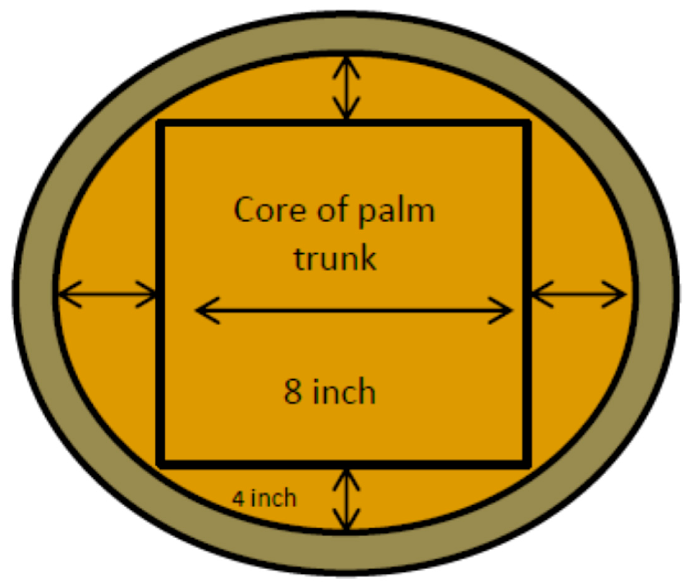
The focus of the present research was to develop a model to prognosticate the fermentation of oil palm trunk sap. Four matured oil palm trunks were acquired from a home-grown plantation of oil palm in Malaysia (Banting-Selangor). The trunks were chopped into 4 sections with the same height (5 feet) [21]. The trunks were also peeled horizontally using an automatic vertical see-saw. The first section from the top of the trunk was labelled as “Upper”, and the following sections were identified as “Middle1”, “Middle2”, and “Bottom”, respectively. Figure 1 shows the cross-section of the oil palm trunk with the details of peeling. To investigate further, before the commencement of the experiment, all sections of the oil palm trunks were stored to be used after 1, 15, 30 and 45 days of storage, respectively.

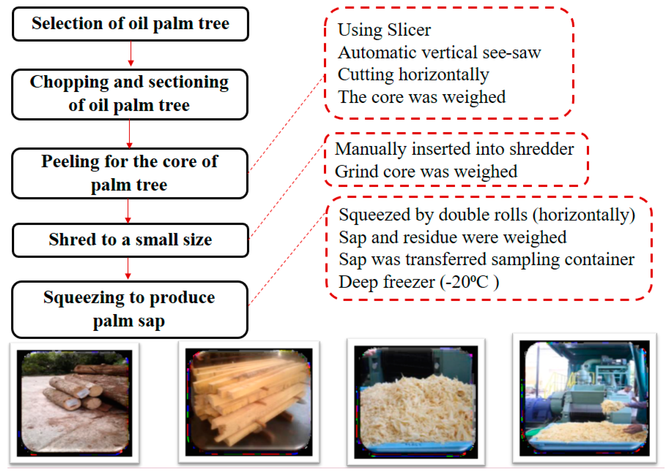
At the beginning of each experiment, the cores of the trunks were shredded into smaller sizes. The weight of the core was measured before and after shredding. A squeezer with double rolls was then used to obtain the oil palm trunk sap (OPTS). The different steps of mechanical pre-treatment on the trunks are shown in Figure 2.

The value for each mass was obtained during the processing of palm sap before and after each processing step was performed, for which the weight of each sample was measured. Assuming that the 4 palm trunks were 900 kg on average when felled, we observed that the cored trunk sections reduced in weight as the storage days increased. During pre-treatment, the stored trunk underwent a few steps to produce palm sap. Firstly, the stored trunk was peeled to remove the hard outer bark or wood waste to reveal the softer parenchyma tissue of the cored trunk section. The softer cored trunk sections were shredded into 1–3 mm pieces before being squeezed to produce palm sap. The squeezed fibrous residue may be used for other application but was considered as waste in this work.

Table 1. Mass balance calculation for palm sap production during pre-treatment.

Storage Time (day)	Section	Initial Trunk (kg)	Cored Trunk (kg)	Wood Waste (kg)	Shredded Trunk (kg)	Oil Palm Trunk Sap (L)	Residue (kg)
1	U	200	103.96	96.04	95.90	58.66	19.46
	M1	200	106.14	93.86	102.55	82.72	10.10
	M2	200	133.25	66.75	130.22	80.56	9.80
	B	300	134.22	165.78	132.16	83.04	12.10
Total		900	477.57	422.43	461.33	309.48	51.52
15	U		100.90		99.14	49.90	38.68
	M1		64.66		59.72	28.18	13.16
	M2		110.20		102.20	64.60	19.10
	B		117.50		115.22	45.73	29.76
Total			393.26		376.28	188.41	100.7
30	U		51.28		45.98	27.78	11.40
	M1		57.42		47.84	26.93	14.28
	M2		73.96		69.10	51.72	10.94
	B		87.74		82.26	57.53	13.44
Total			270.40		245.18	163.96	50.06
45	U		29.32		Not shred	15.32	2.55
	M1		53.70		47.64	20.70	13.16
	M2		66.72		59.88	32.06	10.96
	B		72.64		70.50	10.14	5.52
Total			222.38		178.02	78.22	32.19

U = Upper, M1 = Middle 1, M2 = Middle 2, and B = Bottom.

summarises the mass balance calculation for the trunk sections during palm sap production.

After the sap had been collected, its residues were weighted for further calculation. The OPTS samples were stored and preserved in containers under −20 °C in a freezer. They were later used in different steps of the experiment to complete the fermentation process. The mass balance calculation indicated that the sap volume reduced during the storage time. As a result, the measured OPTS values were 78.22 L, 163.96 L, 188.41 L, and 309.48 L for 45, 30, 15 and 1 storage days respectively. The noteworthy moisture loss was mainly responsible for the reduction of the OPTS volume with time [21].

2.2. Chemical Experiments and Analysis

The analysis for total sugar content was done in the Center of Lipids Engineering and Applied Research (CLEAR) laboratory using high-performance liquid chromatography (HPLC) (1100 series, Agilent Technologies) as well as a refractive index detector with a Shodex SUGAR SP0810 column (NREL, Japan). The alcohol percentage by volume was determined using gas chromatography on a 6890N (Agilent Technologies, USA), which was equipped with a flame ionisation detector and a 7697A headspace sampler as well as a DB-Select-624UI capillary column (30 m × 0.53 mm, 3.00 µm).

A mature (i.e., 25- to 30-year-old) oil palm trunk acts as a source of sap. The sap contains a large volume of sugar and other valuable substances, including amino acids, vitamins, and minerals, as well as organic acids. The moisture content of oil palm trunk sap is reported to be at about 84.2%.

Table 2. Composition of sugars in oil palm trunk sap [23].

Chemical Properties	Concentration (g/L)	Composition of Total Sugar (%)
Sucrose	11.4	6.4
Glucose	150.5	84.2
Fructose	9.3	5.2
Xylose	2.9	1.6
Galactose	2.7	1.5
Rhamnose	1.4	0.8
Other	0.5	0.3
Total	178.7	100

presents the sugar composition in the palm sap squeezed from the middle area of the palm trunk. The table suggests that glucose is the most prominent sugar of the palm sap and represents 84.2% of the total amount of sugar. The sugar extracted from the palm sap acts as a beneficial source for polyhydroxyalkanoate (PHA) and bioethanol production [23,24].

Oil palm trunk sap contains several kinds of amino acids (0.0198% of the total) and vitamins (0.0665% of the total). Oil palm sap’s acidity makes up 0.09706% and is attributed to the multiple organic acids shown in

Table 3. Composition of organic acids from palm sap [25].

Organic Acids	Concentration (µg/g)
Succinic Acid	30.9
Pyruvic Acid	19.0
Malic Acid	371.8
Maleic Acid	119.1
Lactic Acid	1.3
Fumaric Acid	8.1
Citric Acid	380.6
Acetic Acid	39.8
Total	970.6

[25]. The overall sugar content at various mature oil palm tree heights was studied. It was revealed that the upper part and the inner part of the trunk had the richest moisture content, which reduced moving outwards [26].

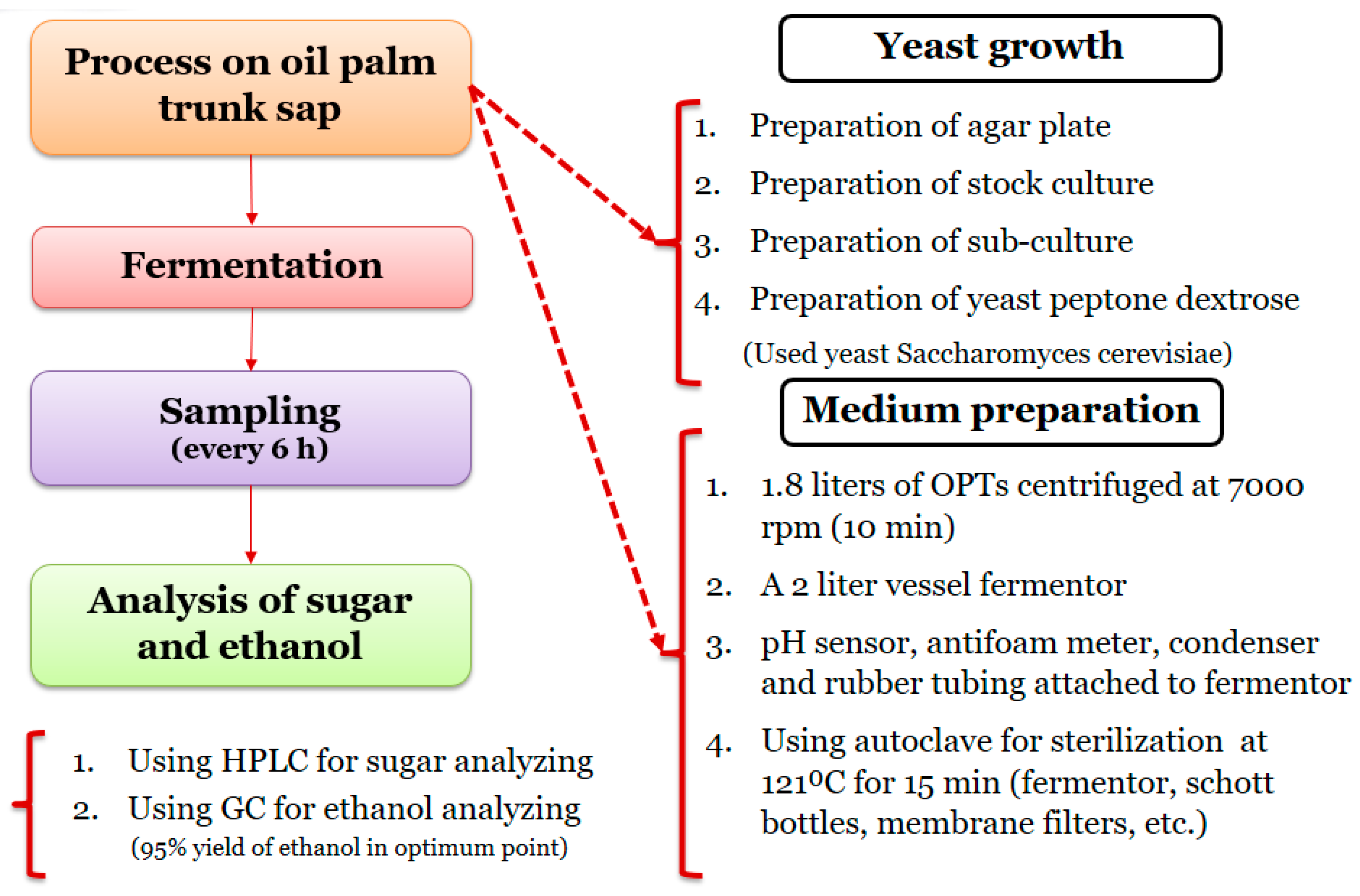
Figure 3 attempts to show the complete applied methodology in the CLEAR laboratory. The results of the HPLC analysis and further calculations indicated an increase in sugar concentration in the OPTS after both 15 and 30 days of storage time. On the contrary, it had decreased in 45-day-old sap. The average sugar concentration and total sugar content of the OPTS for the whole section in respect to the incremental storage times were 55.15 g/L (17.07 kg), 77.53 g/L (14.23 kg), 86.97 g/L (14.25 kg), and 13.07 g/L (1.02 kg), respectively.

As has been shown in

Table 4. Total sugar in palm sap per trunk.

Storage Time (Day)	Total Palm Sap (L)	Average Sugar Concentration (g/L)	Total Sugar (kg)
1	309.48	55.15	17.07
15	188.41	75.53	14.23
30	163.96	86.93	14.25
45	78.22	13.07	1.02

, the increment in sugar content in the first 30 days was large because of the dryness of the trunk sections. The total sugar content in the sap was also almost constant, which was approximately 14 kg/trunk ± 3 kg.

In the yeast fermentation process, the trunk stored for only 1 day was chosen to investigate the effects of both pH and temperature on bioethanol production. The concentration of the substrate, oxygen, and speed rate, as well as time, were considered to be constant in the process. Medium preparation (OPTS) and yeast growth were carried out before commencing the fermentation process. OPTS as a medium was centrifuged at 7000 rpm for 10 min; subsequently, 1.8 L of centrifuged OPTS was used in the fermentation process. A vessel fermenter with a capacity of 2 L was attached, with a pH sensor, antifoam meter condenser, and rubber tubing, and used for the fermentation process. In addition, other equipment included Schott bottles, which were filled with 1 M of sulfuric acid, 1 M sodium hydroxide, and antifoam, along with rubber tubing and membrane filters. The OPTS sample, the fermenter, and the Schott bottles with their contents and attachments were sterilised together using an autoclave (at 121 °C for 15 min). The process of sterilisation ensured that bioethanol production was a result of the yeast that was used (S. cerevisiae), as this process would eliminate organism contamination during fermentation.

To prepare the stock culture and subculture, the equipment and materials used included a refrigerator, an autoclave, an incubator, Petri dishes, agar plates, wire loops, bacteriological agar (HmBg, Germany), Saccharomyces cerevisiae (local), and distilled water were used. Four grams of bacteriological agar mixed in 200 mL distilled water was prepared on the agar plate for yeast growth. The solution was then sterilised at 121 °C for 15 min using an autoclave and was later cooled to reach the temperature of 50–60 °C. Subsequently, Petri dishes were used to gel with the prepared solution at room temperature in sterilised conditions. The stock culture was prepared by spreading yeast into the agar plate and subsequently incubated at 30 °C for 24 h in aerobic conditions. To prolong the yeast cells’ life, the stock culture was cooled and kept at the temperature of 4 °C in the refrigerator. A sterilised (Bunsen burner) and cooled wire loop was used to transfer (zigzag pattern) a small number of yeast colonies from the stock culture to another agar plate to prepare the subculture, which was incubated at 30 °C for 24 h.

Yeast peptone dextrose (YPD), as a common medium, was used for growing yeast by mixing 20 g/L polypeptone, 10 g/L yeast extract, and 20 g/L glucose, which was then dissolved in 200 mL of distilled water. The obtained YPD mixture was autoclaved at 121 °C for 15 min and then cooled at room temperature for 6 h. Sampling was done every 6 h to determine yeast growth by optical density measurement. A UV-Vis spectrophotometer was used to measure the yeast cell growth in 2 mL of the sample transferred into a 2.5 mL glass cuvette. YPD medium was used to prepare inoculum by transferring a loop of yeast, which was grown in subculture, into YPD. An incubator shaker was used for 18 h to fix the temperature at 30 °C for the inoculum. By the 18th hour, 200 mL (10% v/v) of inoculum which contained yeast seed was added to the prepared OPTS (1.8 L).

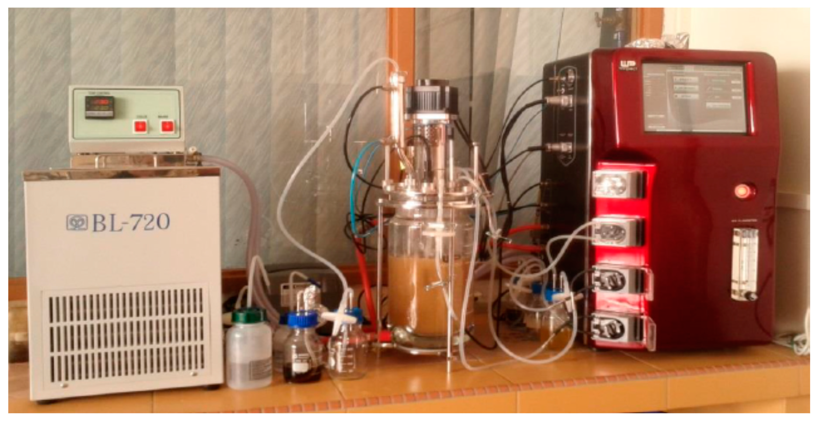
All indicators (antifoam, dissolved oxygen, pH, and temperature), as well as the controller of the impeller, were linked to the monitor. A peristaltic pump was used to transfer 200 mL of the inoculum into the fermenter, which was previously filled with 1.8 L of OPTS. The fermentation process commenced after the inoculum was pumped into the fermenter. During the 24-h fermentation time, a sample of approximately 10 mL of fermented sap was taken every 6 h for further analysis. The bioethanol and sugar analyses were repeated twice for each sample [22]. The set-up for the yeast fermentation in the CLEAR laboratory is shown in Figure 4. In the experimental data, the initial sugar concentration and ethanol concentration can be linearly correlated. The actual value of ethanol produced, compared with the theoretical value, ranged from 13 to 43% using the linear correlation derived during yeast fermentation for an initial sugar concentration of 20 g/L to 146 g/L. However, optimisation of the yeast fermentation operating conditions indicated that the highest ethanol yield of 95% was achieved with an initial sugar concentration of 90 g/L.

2.3. Artificial Intelligence Model

2.3.1. Adaptive Neuro-Fuzzy Inference System

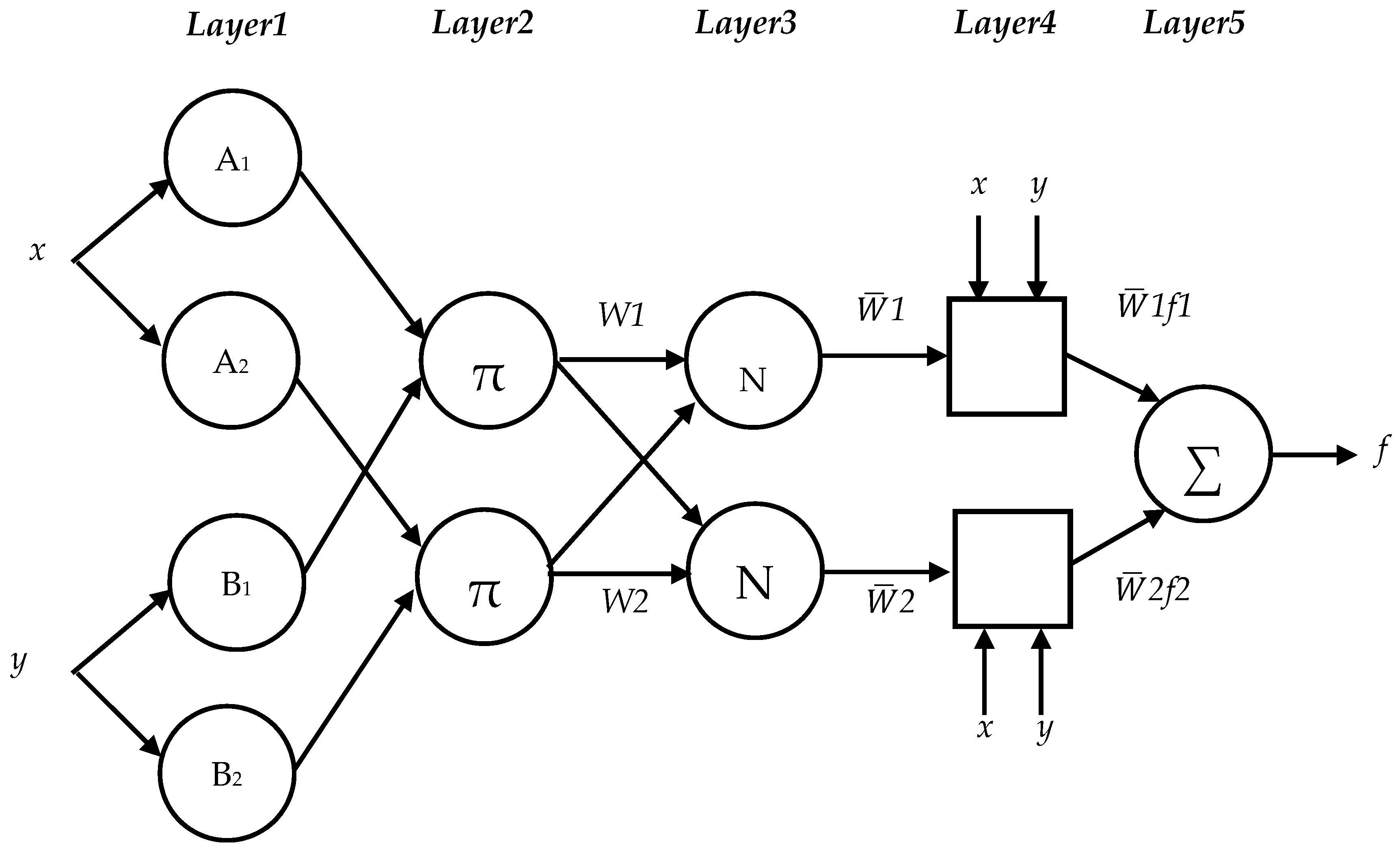
One of the special approaches in the neuro-fuzzy field is the development of adaptive neuro-fuzzy inference systems (ANFIS) that contribute to nonlinear function simulations [28,29,30]. ANFIS is considered to be a hybrid neuro-fuzzy inference expert system that is adaptable with the Takagi–Sugeno-type fuzzy inference system [31] elaborated by Jang [32]. The most common inference system utilised in ANFIS is a first-order Sugeno-type Fuzzy Inference System (FIS) relation command. Throughout the training process, the rule limits, comprising the limits of antecedents and limits of consequents, were adjusted to reduce the output errors to a minimum during the training stage. The procedures can go on without initial knowledge of the consequent parameters. ANFIS can learn the imperative parameters while tuning the membership functions. The structures of an ANFIS and a multilayer feed-forward neural network are alike. However, ANFIS links are capable of showing the signals’ flow direction between nodes, while the links are not associated with any weights.

Figure 5 shows the ANFIS architecture. Squares indicate adaptive nodes, whereas circles indicate fixed nodes in this figure. There are 5 layers in the architecture of ANFIS.

In ANFIS, by using a learning algorithm and updating the set of parameters, the training dataset is fitted. In this research, the parameters of the ANFIS model were tuned and optimised using particle swarm optimisation.

2.3.2. Particle Swarm Optimisation Method

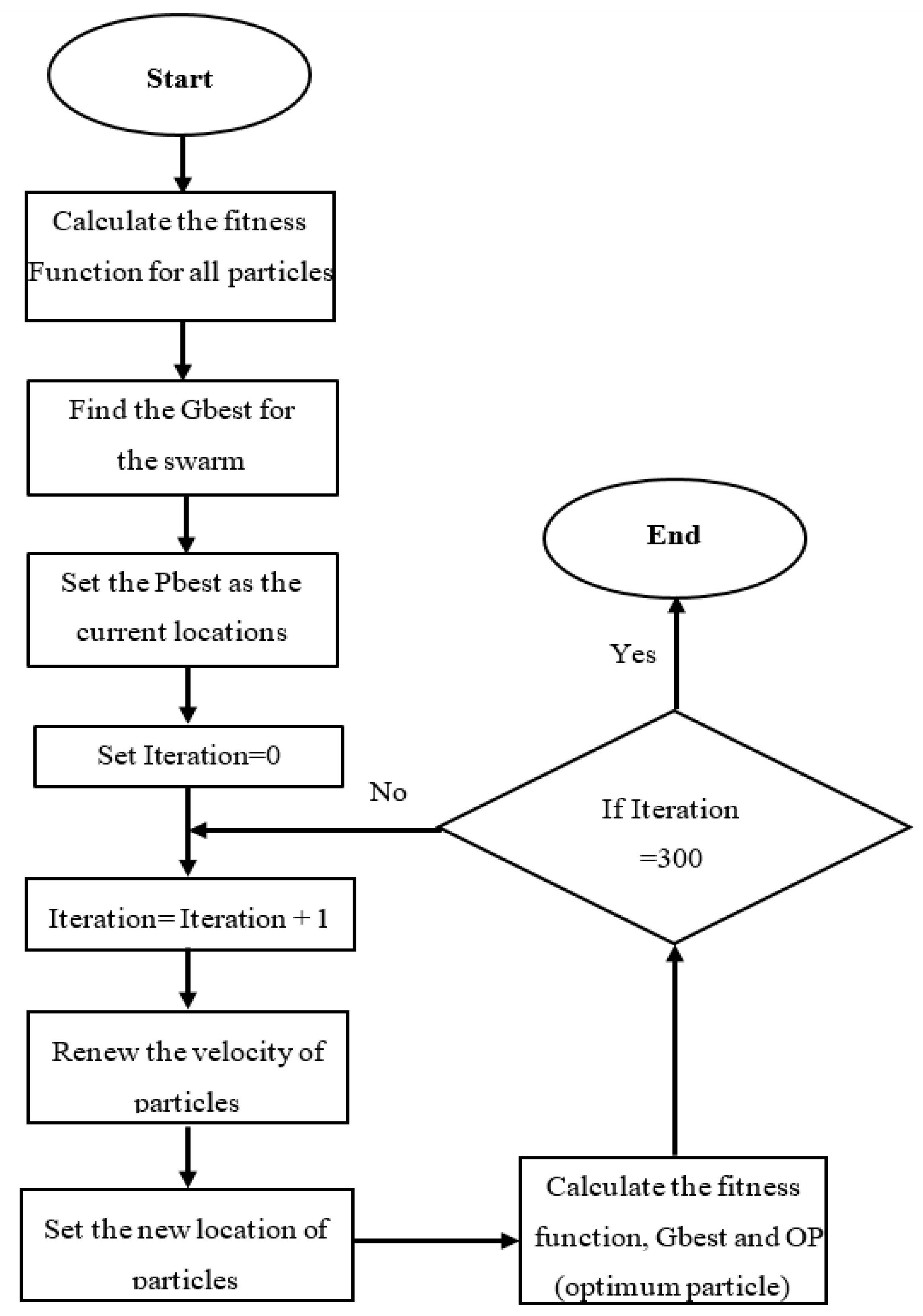
The particle swarm optimisation (PSO) algorithm is mainly based on the movement of the population of particles as a swarm. This movement was inspired by a school of fish or a flock of birds [33,34,35]. In this method, the candidate solutions are called particles, and the optimal solution is reached by updating generations based on the initial population of candidate solutions [36,37]. This method searches for the best solution by sharing social and historical information among the individual candidate solutions [38,39]. The large number of agents in the PSO method is its foremost advantage over other developed optimisation techniques like simulated annealing. The large number of agents makes the PSO method resilient to the local optimum points of the search space. It helps prevent the algorithm from being trapped in the local optimum points. Leading a swarm to the space that comprises the global optimum depends on some social parameters. Two parameters that have been used in PSO approaches are personal best ($Pbest$) and global best ($Gbest$). Figure 6 illustrates a simplified diagram of the PSO method.

2.3.3. Proposed Modelling of Hybrid ANFIS and PSO

This research used the PSO method as an optimisation technique to determine all the best parameters embodied in the ANFIS model to attain a lower prediction error. The objective function for the proposed method was as follows:

$$\mathrm{Min}\mathrm{RMSE}=\sqrt{1/\mathrm{m}{{\displaystyle \sum }}_{j=1}^m{\left[\widehat{F}\left(X_j\right)-Y_j\right]}^2}\sqrt{1/\mathrm{m}{{\displaystyle \sum }}_{j=1}^m{\left[\widehat{F}\left(x_{j1},x_{j2},\dots ,x_{jn}\right)-Y_j\right]}^2}$$

(1)

where $\widehat{F}\left(x_{j1},x_{j2},\dots ,x_{jn}\right)$ is the proposed ANFIS model, $x_{ji}\left(i=1,\dots ,nj=1,2,\dots ,m\right)$ are inputs of the observations for the ANFIS model, $Y_j\left(j=1,2,\dots ,m\right)$ are the outputs of observations, $m$ is the number of observations, $n$ is the number of inputs (input features), and $N$ is the number of membership functions. Therefore (as mentioned in Equation (1)), the objective function of the proposed problem (Equation (2)) can be rewritten as follows:

$$\mathrm{Min}\mathrm{RMSE}=\sqrt{1/\mathrm{m}{{\displaystyle \sum }}_{j=1}^m{\left[\frac{{\sum }_{l=1}^N\left({\sum }_{i=1}^n{\alpha }_i^l{x}_{ji}+{\alpha }_0^l\right)({\prod }_{i=1}^{n}exp\left[-{\left(\frac{x_{ji}-{\gamma }_i^l}{{\beta }_i^l}\right)}^2\right])}{{\sum }_{l=1}^N({\prod }_{i=1}^{n}exp\left[-{\left(\frac{x_{ji}-{\gamma }_i^l}{{\beta }_i^l}\right)}^2\right])}-Y_j\right]}^2}$$

(2)

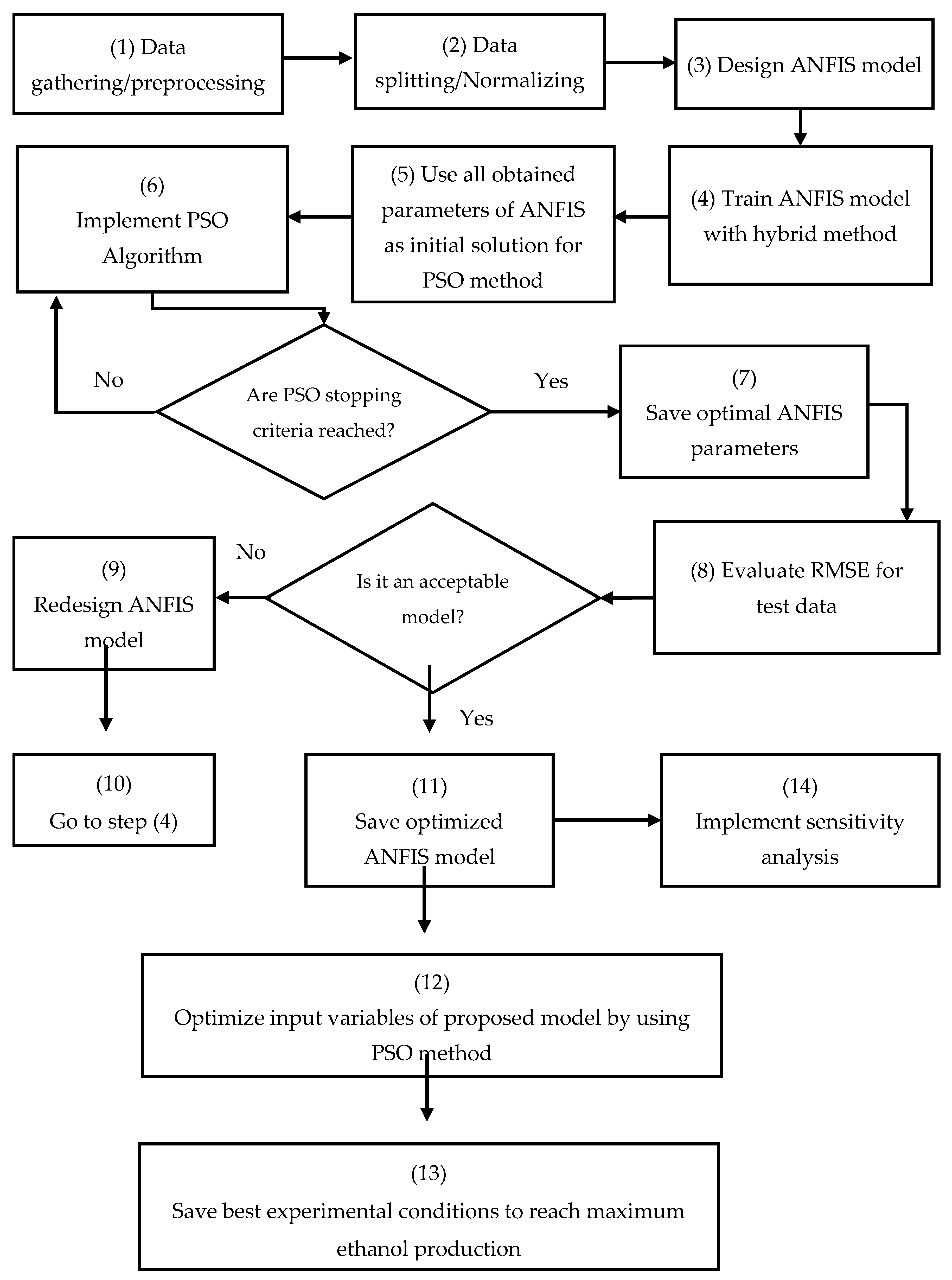
where ${\alpha }_i^l,{\gamma }_i^l,{\beta }_i^l\left(i=1,2,\dots ,n\mathrm{and}l=1,2,\dots ,N\right)$ are the ANFIS parameters which should be set by the PSO method. All steps to reach the maximum bioethanol are summarised in Figure 7. After the PSO method was run, the best parameters of the ANFIS model were obtained with a minimum error of root mean square error (RMSE), then the proposed model were evaluated by checking the data to prevent overfitting.

As mentioned before, there are adjustable parameters in the PSO algorithm such as c₁, c₂, and w, which should be adjusted by the user to achieve a better convergence. The constants c₁ and c₂ denote the weights of the acceleration terms that tend to push a particle toward Pbest and Gbest, respectively. Small values allow a particle to roam far from the target regions. Conversely, large values result in the abrupt movement of particles toward the target regions [40]. In this work, the constants $c_1$ and $c_2$ were both set to 2, following the typical practice in [41].

3. Results and Discussion

This research aimed to consider the accurate prediction of the ANFIS model for bioethanol produced in biomass fermentation of oil palm trunk sap. After the ANFIS model was applied for modelling the experimental results, the input parameters were the fermentation time, the pH, temperature, and total sugar, and the output variable was bioethanol produced in the fermentation of oil palm trunk sap.

Table 5. Summary of the experimental results.

Parameter	Description
Details of Method	Vessel fermenter with 2 L capacity HPLC (Agilent Technologies, USA), was used for sugar content analysis Gas chromatograph, Agilent Technology, USA was used for ethanol analysis
Strain	Saccharomyces cerevisiae
Time (h)	30 and 24
Temperature	30, 25, 35
pH	4, 5, 6
Sugar content (g/L)	Maximum 118.3650
Ethanol (g/L)	Maximum 44.1485
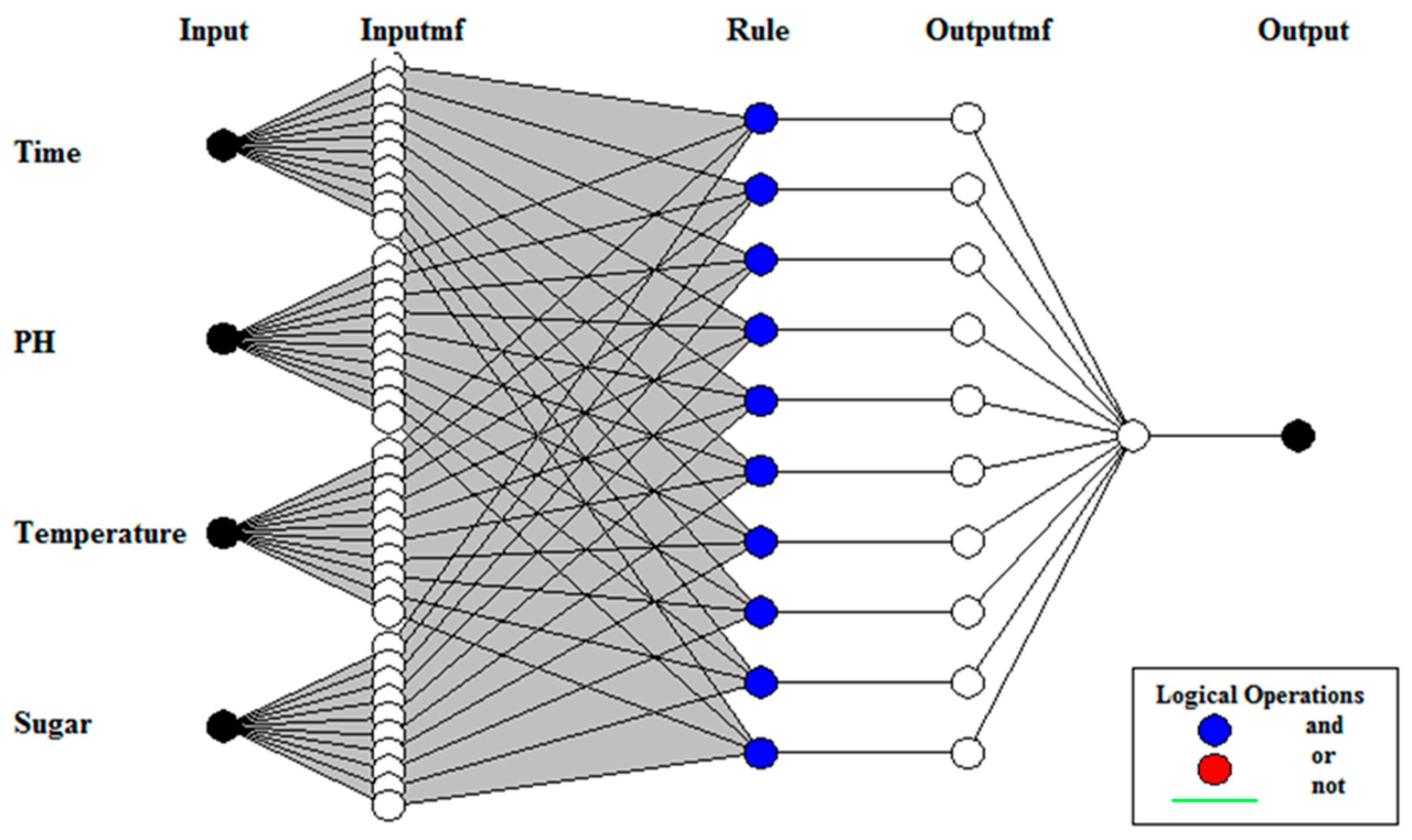
Details of OPT	The OPT was selected from the local plantation, Selangor, Malaysia The OPT was stored 1, 15, 30, 45 days before mechanically squeezing The OPT was 20 feet tall and was divided into four sections: (1) Upper, (2) Middle1, (3) Middle2, and (4) Bottom The OPT sap sample was stored at −20 °C for further analysis

summarises the experimental conditions and results. To achieve the aims of this research, all computational programs were written in MATLAB. The first pre-processing process was executed on all data. As presented in [42], without pre-processing, the results of ANFIS models are not considerable, so using a pre-processing function is unavoidable. This study used the Min and Max normalisation method [43] and the principal component analysis (PCA) method [44,45] as pre-processing processes for the experimental dataset. The dataset was then divided randomly into a test dataset (30%) and a training dataset (70%). Figure 8 presents the structure of the best built ANFIS model for the fermentation process. The black nodes on the furthermost left side have been used to represent the inputs in the first layer. There are 40 nodes with the 10 linked membership functions in the second layer so that the fuzzification procedure with the Gaussian membership function is implemented through this layer.

By using the membership functions in the first layer, a degree is assigned to each input variable which belongs to a proper fuzzy set. In the second layer or fuzzification layer, the fuzzy sets used in the fuzzy rules’ antecedents are represented by neurons. A fuzzification neuron determines a degree for the received crisp inputs to assign each input to the fuzzy set of the neuron. The calculation rules of the fuzzy sets consist of a total of 10 rules, highlighted by the third layer. The fourth layer deals with output membership functions for several rules. The fifth layer is the fourth layer of the output’s aggregation. The defuzzification of the output is displayed in the final layer.

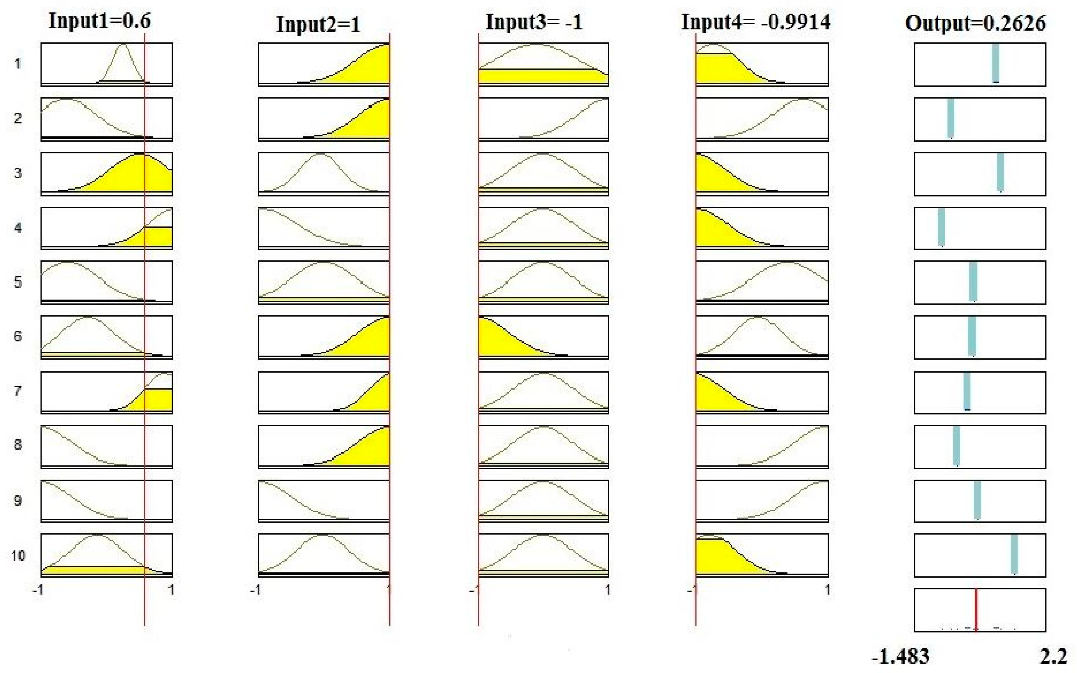
Figure 9 shows the 10 rules, where the different inputs assigned to the model and the respective output are presented. The production of bioethanol can be predicted by diversifying the parameters used as input variables, which are: fermentation time, pH, temperature, and total sugar in the recommended predictive model. For instance, a set of diversified input values of 0.6 (24 h) for the fermentation time and 1 (6), −1 (25 °C), and −0.9914 (0.6357 g/L) for the pH, temperature, and total sugar, respectively, produced a value of 0.2626 (27.8714 g/L) for bioethanol. The amount of bioethanol from the experiment for this set of input values was 0.0667 (24.3005 g/L). The calculation performed for the error percent highlights an error of 1.646% in predicting the amount of bioethanol production. The red line denotes the normalised input values. Its effect on each rule is highlighted in yellow. The output column denotes the output of each rule. The method of combining the output of each rule and defuzzification to establish an output value is shown in the bottom right output plot.

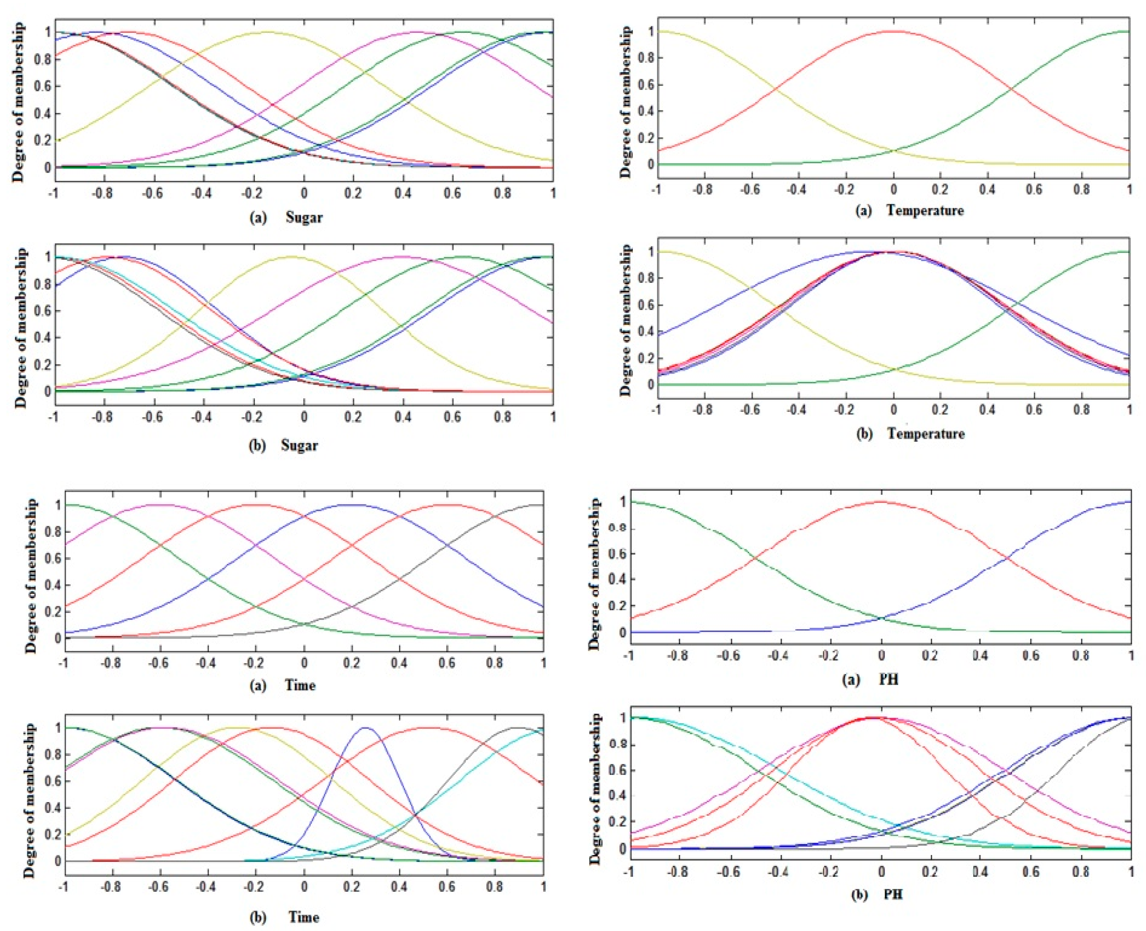
Membership functions were used for input variables initialised by ANFIS before the training process. To achieve the optimal representation of parameters in the initial membership functions for input and output mapping, the parameters were changed by the training process. New parameters altered the shape of the membership function.

With that in mind, the final membership functions would show dissimilar shapes from the initial membership functions. Figure 10 indicates the shapes of the input membership functions before the training process (initial membership functions) and after the training process (finial membership functions) related to the final ANFIS model.

The performance of the models was evaluated by three statistical indices, namely mean square error (MSE), root mean square error (RMSE), and the correlation coefficient (R):

$$MSE=\frac{1}{N}{{\displaystyle \sum }}_{\mathrm{i}=1}^{\mathrm{N}}{\left({\mathrm{y}}_{\mathrm{i}}^{\exp }-{\mathrm{y}}_{\mathrm{i}}^{\mathrm{sim}}\right)}^2$$

(3)

$$RMSE=\sqrt{\frac{1}{N}{{\displaystyle \sum }}_{\mathrm{i}=1}^{\mathrm{N}}{\left({\mathrm{y}}_{\mathrm{i}}^{\exp }-{\mathrm{y}}_{\mathrm{i}}^{\mathrm{sim}}\right)}^2}$$

(4)

$$R=\frac{{\sum }_{x=i}^n\left({\mathrm{y}}_{\mathrm{i}}^{\exp }-{\overline{y}}^{\exp }\right)\left({\mathrm{y}}_{\mathrm{i}}^{\mathrm{sim}}-{\overline{y}}^{\mathrm{sim}}\right)}{\sqrt{{\sum }_{x=i}^n{\left({\mathrm{y}}_{\mathrm{i}}^{\exp }-{\overline{y}}^{\exp }\right)}^2{\left({\mathrm{y}}_{\mathrm{i}}^{\mathrm{sim}}-{\overline{y}}^{\mathrm{sim}}\right)}^2}}$$

(5)

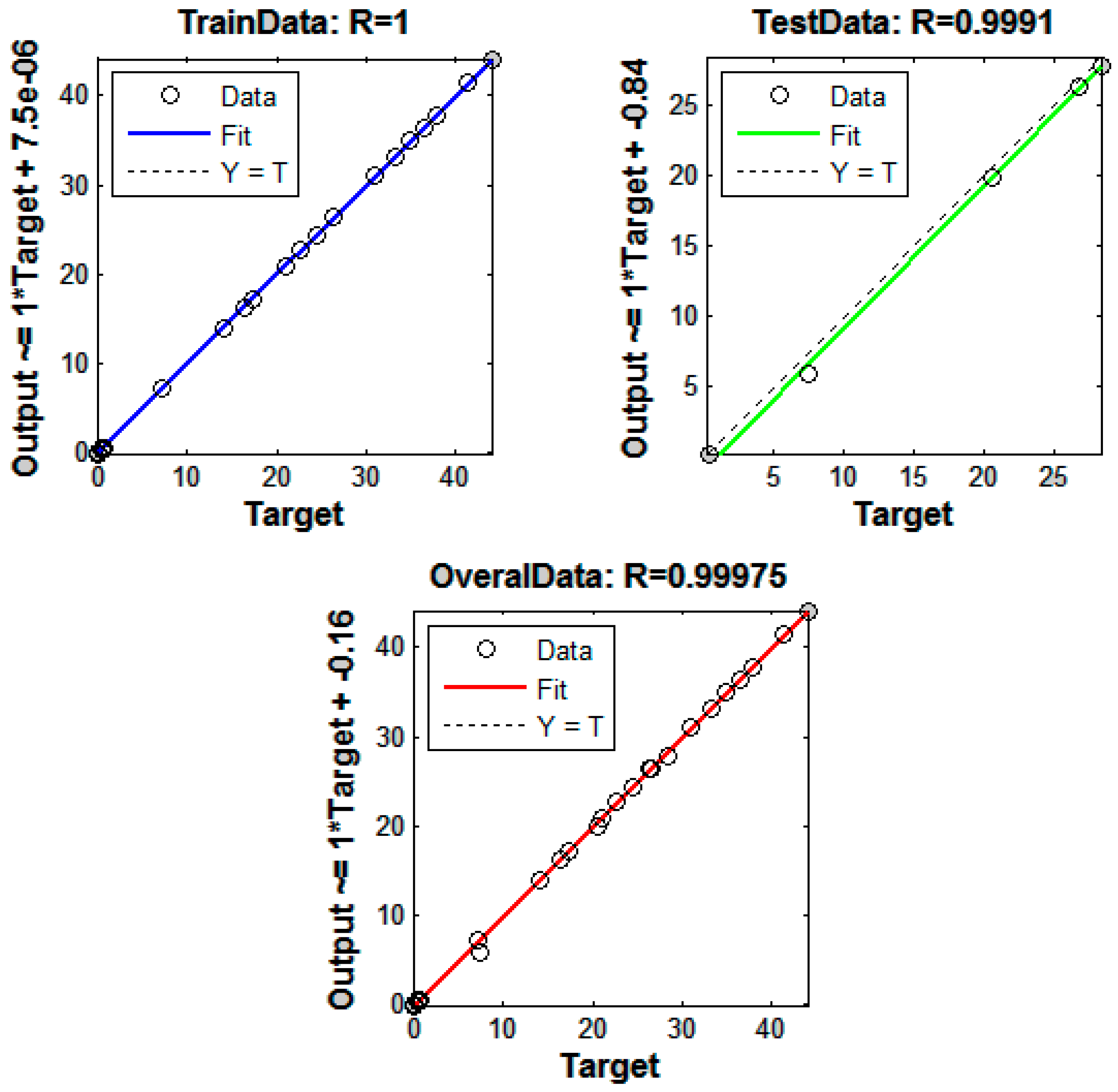
where $y^{\exp }$ is the real output value, $y^{\mathrm{sim}}$ is the predicted output value, and $N$ is the number of the experiments; ${\overline{y}}^{\exp }$ and ${\overline{y}}^{\mathrm{sim}}$ represent the average of real output and the predicted values, respectively. Figure 11 illustrates the statistical performance of the ANFIS model. The regressions of the training and test datasets for the best model were 1 and 0.9991. Moreover,

Table 6. Statistical performance of ANFIS model.

Parameter	Training	Testing	Overall
RMSE	2.52 × 10−6	0.8010	0.3447
RMSE of normalised data	1.14 × 10−6	0.0363	0.0156
MSE	6.37 × 10−10	0.6417	0.1188
MSE of normalised data	1.31 × 10−12	0.0013	2.44 × 10−4
R	1	0.9991	0.9997

shows the error rates of the proposed model obtained when the normalisation methods were used. The lowest RMSE for the training and test datasets were 1.14 × 10⁻⁶ and 0.0363, respectively. They proved that the validity of the proposed model is acceptable and that the proposed model can be used as a viable predictive model.

3.1. Effect of the Input Variables on the Response

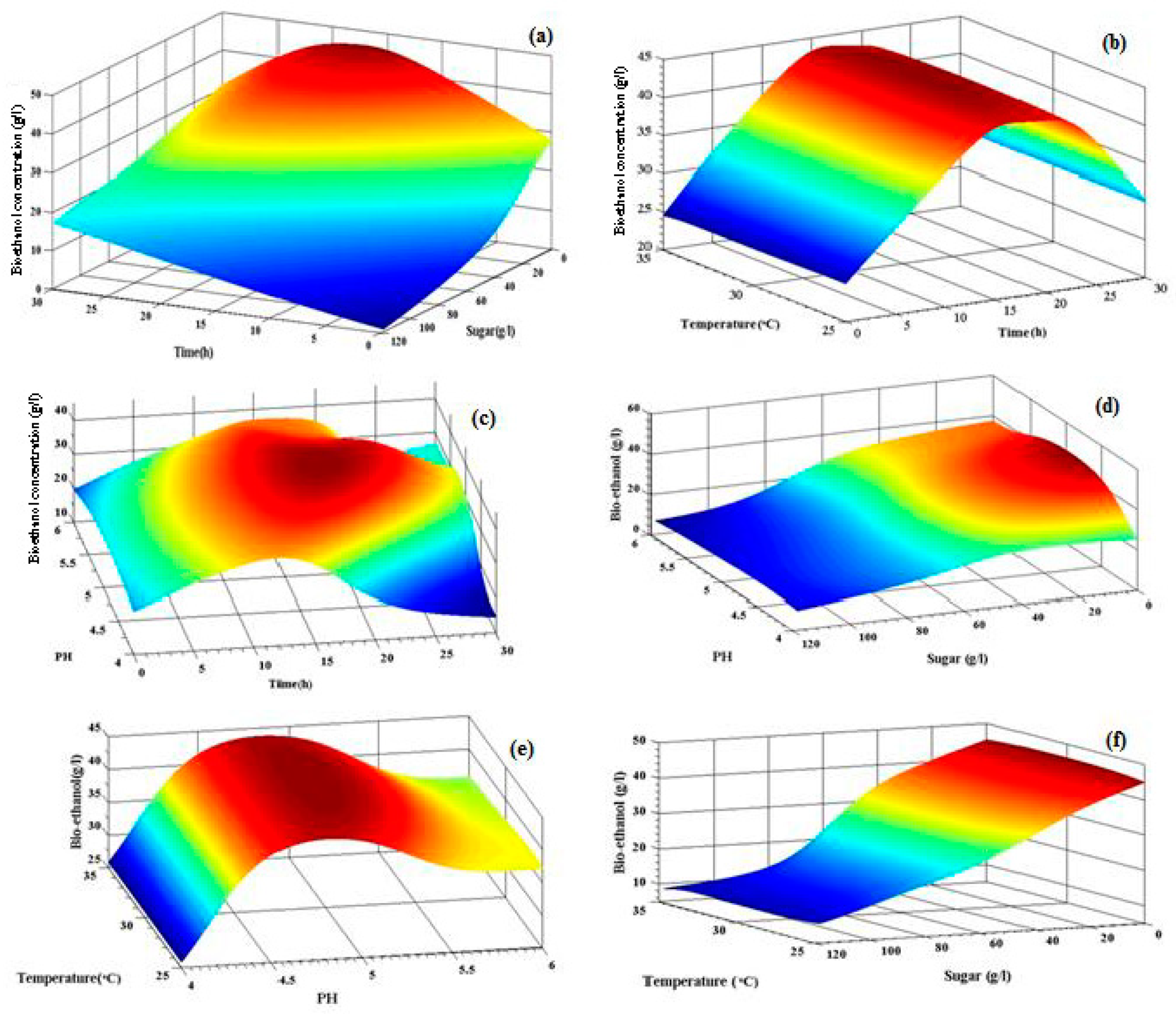
The developed ANFIS model was used to identify the relationship among variables. Figure 12a–f shows the bioethanol production forecasted by the proposed ANFIS model when two effective parameters have been changed in their range, and the other parameters considered as inputs have been kept constant. In the experimental results, 44.1485 g/L was the maximum amount of produced bioethanol and 8.2639 g/L was the amount of sugar content that remained after 18 h of fermentation time at 30 °C, while the pH value was 5.

Figure 12a shows the surface plot for the sugar concentration and time in terms of the bioethanol concentration predicted by the ANFIS model, while the temperature and pH were fixed at 30 °C and 5 respectively. The bioethanol concentration kept increasing to reach the peak point while the sugar content was mitigated by the time. The optimum fermentation time to convert more sugar content into bioethanol could be 14–21 h.

The evolution of bioethanol in terms of the temperature and time is shown in Figure 12b, where all other variables are fixed. Bioethanol production was dependent on the time until it reached the maximum peak point. A visible decrease in bioethanol production happened with time. Time is a more important variable, so changing the temperature from 25 °C to 35 °C had a lesser effect on bioethanol production. The effect of temperature on the fermentation process depends on the background strain’s thermal tolerance in the fermentation process. Therefore, the optimal temperature will be changed by using different strains. From this point of view, using a higher temperature than the thermal strain’s tolerance prevents strain growth and results in low sugar consumption and, consequently, a low final bioethanol concentration.

Figure 12c shows a surface plot for pH and time in terms of the predicted bioethanol concentration. This figure presents the pH as having a significant effect on the bioethanol production at lower limits of time. Figure 12c illustrates the range of precise pH values that lead to the maximum bioethanol production in different fermentation times. The values of pH from 4.4 to 5.6 are the looked-for values to produce maximum bioethanol in almost 12 to 24 h of fermentation.

The surface plot for sugar concentration and pH in terms of the predicted bioethanol concentration in 30 h of fermentation time is shown in Figure 12d and proves that pH changing in the range of 4 to 6 has a significant effect on the fermentation process, while almost more than two-thirds of the sugar was consumed and converted to bioethanol. Moreover, Figure 12d shows that the maximum bioethanol production can be found when the pH is around 5.

Surface plots of temperature and pH are shown in Figure 12e, which shows that changing the temperature in the range of 25 °C to 35 °C has less effect on bioethanol production, while bioethanol production is more dependent on the pH value.

The surface plot concerning the temperature and sugar is shown in Figure 12f. The figure indicates that increasing ethanol production is not dependent on changing the temperature in the range of 25 °C to 35 °C. It proves that this range is the optimum interval for the temperature and leads to producing the maximum volume of bioethanol. Bioethanol production increases until the sugar content is high compared with the presence of low sugar, whereby the bioethanol production keeps decreasing. This could be because of the loss of yeast viability and, consequently, the declining rate of fermentation. In yeast fermentation, the increasing concentration of bioethanol is the most prevalent stress on the cells and can have adverse consequences for fermentation and bioethanol yields [46].

3.2. Optimisation of Experimental Conditions

The proposed ANFIS model was optimised to find the best experimental conditions to get the maximum bioethanol concentration. As mentioned in Equation (1), the objective function of the proposed model can be written as follows:

$$\mathrm{Max}\tilde{Y}=\tilde{F}\left(X\right)=\frac{{\sum }_{l=1}^N\left({\sum }_{i=1}^n{\alpha }_i^l{x}_i+{\alpha }_0^l\right)({\prod }_{i=1}^{n}exp\left[-{\left(\frac{x_i-{\gamma }_i^l}{{\beta }_i^l}\right)}^2\right])}{{\sum }_{l=1}^N({\prod }_{i=1}^{n}exp\left[-{\left(\frac{x_i-{\gamma }_i^l}{{\beta }_i^l}\right)}^2\right])}$$

(6)

where $\tilde{Y}$ is the approximate value of bioethanol and $\tilde{F}\left(X\right)$ is the best predicted ANFIS model of the fermentation process so that all parameters were optimised and justified. X is the independent variables’ vector in the proposed fermentation process; $x_i,i=1,2,\dots ,n$ are input features of the proposed fermentation process (such as fermentation time, pH, temperature, and the amount of sugar), which should be set; $N$ is the number of membership functions; $n$ is the number of input features; and ${\alpha }_i^l,{\gamma }_i^l,{\beta }_i^l$ are ANFIS parameters justified and fixed using the PSO method.

The values of the input variables$x_i,\mathrm{where}i=1,2,\dots ,n$, should be found. The PSO method was utilised to find the maximum bioethanol production because of a circumstance that was never examined in the laboratory as one of the chosen input variables.

Table 7. The optimized results.

PSO Parameters
Number of Particles	Number of Dimensions		C1	C2	Maximum Iteration		Inertia Weight (W)
200	4		2	2	300		0.4 ≤ W ≤ 1.2
Optimised Results
Time (h)	pH	Temperature (°C)		Total Sugar (g/L)		Bioethanol (g/L)
16.1845	4.54	27.3407		1.3588		44.1485
Experimental Results
Time (h)	pH	Temperature (°C)		Total Sugar (g/L)		Bioethanol (g/L)
18	5	30		8.2639		44.1485

shows the PSO optimisation results for the fermentation processes. The results of the PSO method showed that the maximum concentration of bioethanol was achieved in almost 16–18 h when the values of pH and temperature were fixed at 4.54 and 27.34 °C, respectively.

3.3. Sensitivity Analysis

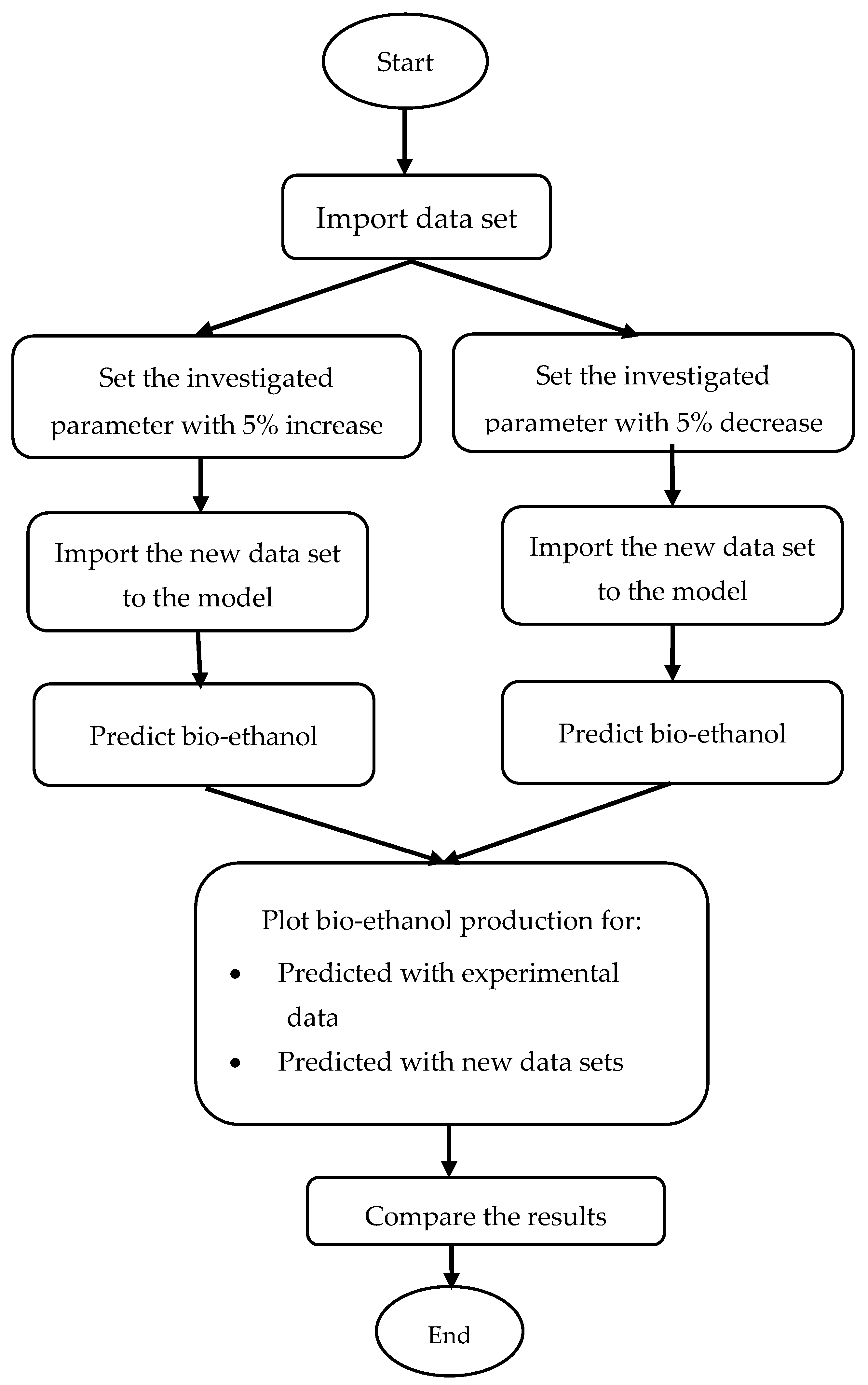
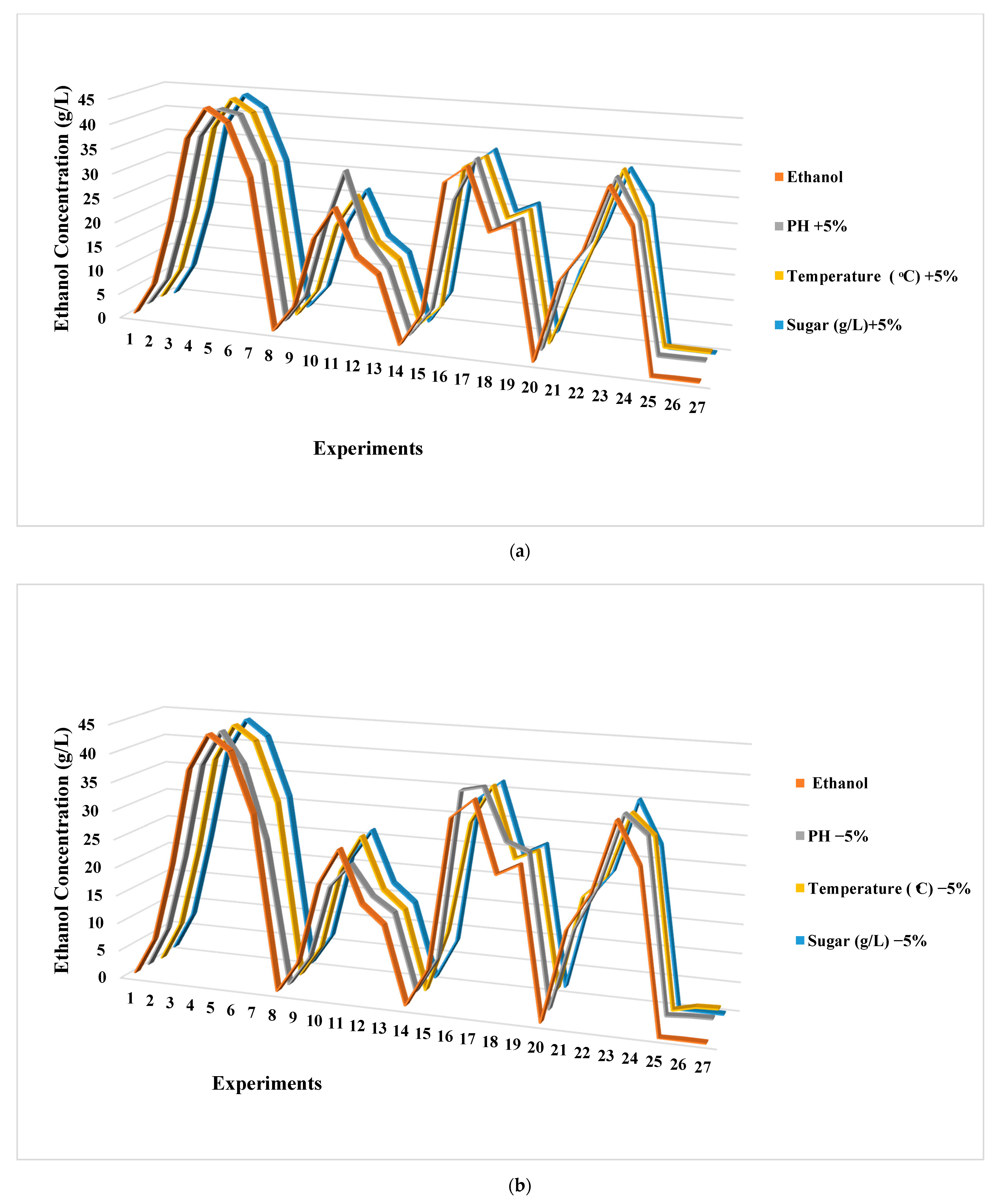
The model outputs are sensitive to changes in the input variables. Information about these sensitivities is very useful for monitoring and improving the studied processes. This information can be achieved by using different sensitivity analysis methods. The graphical method is one of methods and was applied to examine the sensitivity of the outputs to the changes in each input variable. In this method, the effect of each input parameter on bioethanol concentration was studied separately by the prepared scatter graphs. For more description, an input parameter was selected and changed by ±5%, while the other variables were kept constant. The sensitivity of the selected input parameter using the obtained neuro-fuzzy models was then investigated. The sensitivity analysis diagram for the model is shown in Figure 13. In Figure 14a,b, the grey plots have the most variation rather than the other plots showing that pH has a more significant effect on bioethanol concentration in comparison with temperature and sugar content. At the second level, the temperature can be considered an important parameter controlling the fermentation process.

4. Conclusions

In this research, first, palm oil trunk sap (as a new and noticeable source for producing bioethanol in Malaysia) was prepared and fermented in the CLEAR laboratory by using the fermentation set-up. Attempts were made to design an optimised ANFIS model to predict and simulate the bioethanol concentration in the fermentation of oil palm trunk sap, which was tuned and optimised using the PSO method. The four input variables were the fermentation time, the amount of total sugar, temperature, and pH. The results showed the coefficient of determination, mean square error, and root mean square error between the experimental and predicted values as follows: 0.9991, 0.0013, and 0.0363, respectively. The optimum experimental conditions to reach maximum bioethanol production were 27.34 °C, 4.54 pH, and 16.18 h, while 1.3588 g/L sugar remained.

The findings demonstrated that the proposed ANFIS model is a valuable model that can be used to predict the bioethanol concentration in the fermentation process. It could be applied by scientists and engineers to predict the amount of bioethanol concentration under various conditions without performing real experimental measurements. Prediction of bioethanol produced in other nonfood fermentation processes (such as corn stover and palm oil plantations) by the proposed model will be done as later research.

References

- Kwiatkowski, J.R.; McAloon, A.J.; Taylor, F.; Johnston, D.B. Modeling the process and costs of fuel ethanol production by the corn dry-grind process. Ind. Crop. Prod. 2006, 23, 288–296. [Google Scholar] [CrossRef]
- Lübken, M.; Gehring, T.; Wichern, M. Microbiological fermentation of lignocellulosic biomass: Current state and prospects of mathematical modeling. Appl. Microbiol. Biotechnol. 2010, 85, 1643–1652. [Google Scholar] [CrossRef]
- Yang, Q.; Gao, H.; Zhang, W.; Chi, Z.; Yi, Z. A new data-driven modeling method for fermentation processes. Chemom. Intell. Lab. Syst. 2016, 152, 88–96. [Google Scholar] [CrossRef]
- bin Mohd Zain, M.Z.; Kanesan, J.; Kendall, G.; Chuah, J.H. Optimization of fed-batch fermentation processes using the Backtracking Search Algorithm. Expert Syst. Appl. 2018, 91, 286–297. [Google Scholar] [CrossRef]
- Lübken, M.; Wichern, M.; Schlattmann, M.; Gronauer, A.; Horn, H. Modelling the energy balance of an anaerobic digester fed with cattle manure and renewable energy crops. Water Res. 2007, 41, 4085–4096. [Google Scholar] [CrossRef] [PubMed]
- Udwadia, F.; Farahani, A. Accelerated Runge-Kutta Methods. Discret. Dyn. Nat. Soc. 2008, 2008, 1–38. [Google Scholar] [CrossRef]
- Nasrah, N.S.M.; Zahari, M.A.K.M.; Masngut, N.; Ariffin, H. Statistical optimization for biobutanol production by clostridium acetobutylicum ATCC 824 from Oil Palm Frond (OPF) juice using response surface methodology. MATEC Web Conf. 2017, 111, 03001. [Google Scholar] [CrossRef] [Green Version]
- Nath, K.; Das, D. Modeling and optimization of fermentative hydrogen production. Bioresour. Technol. 2011, 102, 8569–8581. [Google Scholar] [CrossRef] [PubMed]
- Kyazze, G.; Popov, A.; Dinsdale, R.; Esteves, S.; Hawkes, F.; Premier, G.; Guwy, A. Influence of catholyte pH and temperature on hydrogen production from acetate using a two chamber concentric tubular microbial electrolysis cell. Int. J. Hydrogen Energy 2010, 35, 7716–7722. [Google Scholar] [CrossRef]
- Jana, A.; Maity, C.; Halder, S.K.; Mondal, K.C.; Pati, B.R.; Mohapatra, P.K.D. Tannase production by Penicillium purpurogenum PAF6 in solid state fermentation of tannin-rich plant residues following OVAT and RSM. Appl. Biochem. Biotechnol. 2012, 167, 1254–1269. [Google Scholar] [CrossRef] [PubMed]
- Mandenius, C.F.; Brundin, A. Bioprocess optimization using design-of-experiments methodology. Biotechnol. Prog. 2008, 24, 1191–1203. [Google Scholar] [CrossRef]
- Kana, E.G.; Oloke, J.; Lateef, A.; Adesiyan, M. Modeling and optimization of biogas production on saw dust and other co-substrates using artificial neural network and genetic algorithm. Renew. Energy 2012, 46, 276–281. [Google Scholar] [CrossRef]
- Wang, Y.-X.; Lu, Z.-X. Optimization of processing parameters for the mycelial growth and extracellular polysaccharide production by Boletus spp. ACCC 50328. Process Biochem. 2005, 40, 1043–1051. [Google Scholar] [CrossRef]
- Lotfy, W.A.; Ghanem, K.M.; El-Helow, E.R. Citric acid production by a novel Aspergillus niger isolate: II. Optimization of process parameters through statistical experimental designs. Bioresour. Technol. 2007, 98, 3470–3477. [Google Scholar] [CrossRef]
- Wang, J.; Wan, W. Optimization of fermentative hydrogen production process using genetic algorithm based on neural network and response surface methodology. Int. J. Hydrogen Energy 2009, 34, 255–261. [Google Scholar] [CrossRef]
- Nelofer, R.; Ramanan, R.N.; Abd Rahman, R.N.Z.R.; Basri, M.; Ariff, A.B. Comparison of the estimation capabilities of response surface methodology and artificial neural network for the optimization of recombinant lipase production by E. coli BL21. J. Ind. Microbiol. Biotechnol. 2012, 39, 243–254. [Google Scholar] [CrossRef]
- Yan, Y.; Borhani, T.N.; Clough, P.T. Chapter 14 machine learning applications in chemical engineering. In Machine Learning in Chemistry: The Impact of Artificial Intelligence; The Royal Society of Chemistry: Cambridge, UK, 2020; pp. 340–371. [Google Scholar]
- Ezzatzadegan, L.; Morad, N.A.; Yusof, R. Prediction and optimization of ethanol concentration in biofuel production using fuzzy neural network. J. Teknol. 2016, 78. [Google Scholar] [CrossRef] [Green Version]
- Borhani, T.N.; García-Muñoz, S.; Luciani, C.V.; Galindo, A.; Adjiman, C.S. Hybrid QSPR models for the prediction of the free energy of solvation of organic solute/solvent pairs. Phys. Chem. Chem. Phys. 2019, 21, 13706–13720. [Google Scholar] [CrossRef] [PubMed] [Green Version]
- Babamohammadi, S.; Shamiri, A.; Nejad Ghaffar Borhani, T.; Shafeeyan, M.S.; Aroua, M.K.; Yusoff, R. Solubility of CO2 in aqueous solutions of glycerol and monoethanolamine. J. Mol. Liq. 2018, 249, 40–52. [Google Scholar] [CrossRef]
- Morad, N.A.; Ibrahim, W.A.; Muda, N.S.; Shirai, Y.; Aziz, M.K.A.; Lam, H.L. Utilization of felled oil palm trunk: Trunk sections storage on oil palm sap production. In Proceedings of the 2015 10th Asian Control Conference (ASCC), Sabah, Malaysia, 31 May–3 June 2015; pp. 1–5. [Google Scholar]
- Muda, N.S. Utilization of Oil Palm Trunk Sap for Bioethanol Production through Natural and Yeast Fermentation; Universiti Teknologi Malaysia: Johor Bahru, Malaysia, 2015. [Google Scholar]
- Yamada, H.; Tanaka, R.; Sulaiman, O.; Hashim, R.; Hamid, Z.; Yahya, M.; Kosugi, A.; Arai, T.; Murata, Y.; Nirasawa, S. Old oil palm trunk: A promising source of sugars for bioethanol production. Biomass Bioenergy 2010, 34, 1608–1613. [Google Scholar] [CrossRef]
- Lokesh, B.E.; Hamid, Z.A.A.; Arai, T.; Kosugi, A.; Murata, Y.; Hashim, R.; Sulaiman, O.; Mori, Y.; Sudesh, K. Potential of oil palm trunk sap as a novel inexpensive renewable carbon feedstock for polyhydroxyalkanoate biosynthesis and as a bacterial growth medium. Clean–Soil Air Water 2012, 40, 310–317. [Google Scholar] [CrossRef]
- Kosugi, A.; Tanaka, R.; Magara, K.; Murata, Y.; Arai, T.; Sulaiman, O.; Hashim, R.; Hamid, Z.A.A.; Yahya, M.K.A.; Yusof, M.N.M. Ethanol and lactic acid production using sap squeezed from old oil palm trunks felled for replanting. J. Biosci. Bioeng. 2010, 110, 322–325. [Google Scholar] [CrossRef]
- Murai, K.; Kondo, R. Extractable sugar contents of trunks from fruiting and nonfruiting oil palms of different ages. J. Wood Sci. 2011, 57, 140–148. [Google Scholar] [CrossRef]
- Ezzat Zadegan, L. Modelling and Optimization of Fermentation Process to Produce Bio-Ethanol from Oil Palm Trunk Sap and Corn Stover; Universiti Teknologi Malaysia: Johor Bahru, Malaysia, 2018. [Google Scholar]
- Cakmakci, M. Adaptive neuro-fuzzy modelling of anaerobic digestion of primary sedimentation sludge. Bioprocess Biosyst. Eng. 2007, 30, 349–357. [Google Scholar] [CrossRef]
- Xie, Q.; Ni, J.-q.; Su, Z. A prediction model of ammonia emission from a fattening pig room based on the indoor concentration using adaptive neuro fuzzy inference system. J. Hazard. Mater. 2017, 325, 301–309. [Google Scholar] [CrossRef] [PubMed]
- Najafi, B.; Faizollahzadeh Ardabili, S. Application of ANFIS, ANN, and logistic methods in estimating biogas production from spent mushroom compost (SMC). Resour. Conserv. Recycl. 2018, 133, 169–178. [Google Scholar] [CrossRef]
- Sugeno, M.; Kang, G.T. Structure identification of fuzzy model. Fuzzy Sets Syst. 1988, 28, 15–33. [Google Scholar] [CrossRef]
- Jang, J.S.R. ANFIS: Adaptive-network-based fuzzy inference system. IEEE Trans. Syst. Man Cybern. 1993, 23, 665–685. [Google Scholar] [CrossRef]
- Potter, C.W.; Negnevitsky, M. Very short-term wind forecasting for Tasmanian power generation. IEEE Trans. Power Syst. 2006, 21, 965–972. [Google Scholar] [CrossRef]
- Poli, R.; Kennedy, J.; Blackwell, T. Particle swarm optimization. Swarm Intell. 2007, 1, 33–57. [Google Scholar] [CrossRef]
- Del Valle, Y.; Venayagamoorthy, G.K.; Mohagheghi, S.; Hernandez, J.-C.; Harley, R.G. Particle swarm optimization: Basic concepts, variants and applications in power systems. IEEE Trans. Evol. Comput. 2008, 12, 171–195. [Google Scholar] [CrossRef]
- Karkevandi-Talkhooncheh, A.; Hajirezaie, S.; Hemmati-Sarapardeh, A.; Husein, M.M.; Karan, K.; Sharifi, M. Application of adaptive neuro fuzzy interface system optimized with evolutionary algorithms for modeling CO2-crude oil minimum miscibility pressure. Fuel 2017, 205, 34–45. [Google Scholar] [CrossRef]
- Castillo, O. Type-2 Fuzzy Logic in Intelligent Control Applications; Springer Publishing Company, Incorporated: New York, NY, USA, 2011; p. 200. [Google Scholar]
- Yuan, S.-F.; Chu, F.-L. Fault diagnostics based on particle swarm optimisation and support vector machines. Mech. Syst. Signal Process. 2007, 21, 1787–1798. [Google Scholar] [CrossRef]
- Chen, M.-Y. A hybrid ANFIS model for business failure prediction utilizing particle swarm optimization and subtractive clustering. Inf. Sci. 2013, 220, 180–195. [Google Scholar] [CrossRef]
- Chen, P.-H. Particle Swarm Optimization for Power Dispatch with Pumped Hydro; INTECH Open Access Publisher: London, UK, 2009. [Google Scholar]
- Bakyani, A.E.; Sahebi, H.; Ghiasi, M.M.; Mirjordavi, N.; Esmaeilzadeh, F.; Lee, M.; Bahadori, A. Prediction of CO2–oil molecular diffusion using adaptive neuro-fuzzy inference system and particle swarm optimization technique. Fuel 2016, 181, 178–187. [Google Scholar] [CrossRef]
- Ezzatzadegan, L. Neuro-Fuzzy Kinetic Modeling of Propylene Polymerization; Universiti Teknologi Malaysia: Johor Bahru, Malaysia, 2011. [Google Scholar]
- Dahbi, S.; Ezzine, L.; El Moussami, H. Modeling of surface roughness in turning process by using Artificial Neural Networks. In Proceedings of the 2016 3rd International Conference on Logistics Operations Management (GOL), Fez, Morocco, 23–25 May 2016; pp. 1–6. [Google Scholar]
- Bastianoni, S.; Pulselli, F.M.; Focardi, S.; Tiezzi, E.B.P.; Gramatica, P. Correlations and complementarities in data and methods through Principal Components Analysis (PCA) applied to the results of the SPIn-Eco Project. J. Environ. Manag. 2008, 86, 419–426. [Google Scholar] [CrossRef]
- Dubey, A.K.; Yadava, V. Multi-objective optimization of Nd:YAG laser cutting of nickel-based superalloy sheet using orthogonal array with principal component analysis. Opt. Lasers Eng. 2008, 46, 124–132. [Google Scholar] [CrossRef]
- Ding, M.-Z.; Cheng, J.-S.; Xiao, W.-H.; Qiao, B.; Yuan, Y.-J. Comparative metabolomic analysis on industrial continuous and batch ethanol fermentation processes by GC-TOF-MS. Metabolomics 2009, 5, 229. [Google Scholar] [CrossRef]
Figure 1.
The cross-section of the oil palm trunk [22].
Figure 2.
Details of the mechanical pre-treatment of palm oil trunks to obtain oil palm trunk sap (OPTS).
Figure 3.
Methodology applied in the Center of Lipids Engineering and Applied Research (CLEAR) laboratory.
Figure 5.
Adaptive-Network-Fuzzy Inference System (ANFIS) structure [33].
Figure 6.
Flowchart of particle swarm optimisation (PSO) [27].
Figure 7.
Proposed hybrid PSO and ANFIS modelling in this study.
Figure 8.
Structure of the proposed ANFIS model based on experimental data.
Figure 9.
Diagram of ANFIS rules: Input 1 (fermentation time), Input 2 (pH), Input 3 (temperature), Input 4 (total sugar), and Output (bioethanol).
Figure 10.
(a) Initial and (b) final membership functions for sugar, temperature, time, and pH in ANFIS modelling.
Figure 11.
Regression results for the training, test, and all datasets.
Figure 12.
Surface plots of bioethanol (g/L) evolution respect to time vs. sugar (a), temperature vs. time (b), time vs. pH (c), pH vs. sugar (d), temperature vs. pH (e), and sugar vs. temperature (f) in ANFIS modelling.
Figure 13.
Flowchart of the sensitivity analysis [27].
Figure 14.
Comparison of effects of (+ 5%) variation (a) and (− 5%) variation (b) in different variables on bioethanol concentration.