A Genetic Algorithm Approach as a Self-Learning and Optimization Tool for PV Power Simulation and Digital Twinning


1
Fraunhofer ISE, Fraunhofer Institute for Solar Energy Systems, Heidenhofstrasse 2, 79110 Freiburg, Germany
2
Department of Applied Mathematics and Computer Science (DTU Compute), Technical University of Denmark, DK-2800 Lyngby, Denmark
*
Author to whom correspondence should be addressed.
Energies 2020, 13(24), 6712; https://doi.org/10.3390/en13246712
Submission received: 6 November 2020
/
Revised: 14 December 2020
/
Accepted: 17 December 2020
/
Published: 19 December 2020
(This article belongs to the Special Issue Solar Radiation Forecasting and Photovoltaic Systems Performance Modeling)
Abstract
:A key aspect for achieving a high-accuracy Photovoltaic (PV) power simulation, and reliable digital twins, is a detailed description of the PV system itself. However, such information is not always accurate, complete, or even available. This work presents a novel approach to learn features of unknown PV systems or subsystems using genetic algorithm optimization. Based on measured PV power, this approach learns and optimizes seven PV system parameters: nominal power, tilt and azimuth angles, albedo, irradiance and temperature dependency, and the ratio of nominal module to nominal inverter power (DC/AC ratio). By optimizing these parameters, we create a digital twin that accurately reflects the actual properties and behaviors of the unknown PV systems or subsystems. To develop this approach, on-site measured power, ambient temperature, and satellite-derived irradiance of a PV system located in south-west Germany are used. The approach proposed here achieves a mean bias error of about 10% for nominal power, 3° for azimuth and tilt angles, between 0.01%/C and 0.09%/C for temperature coefficient, and now-casts with an accuracy of around 6%. In summary, we present a new solution to parametrize and simulate PV systems accurately with limited or no previous knowledge of their properties and features.
1. Introduction
Photovoltaic cumulative installed capacity in 2019 added up to 512.3 GW, globally. Over 276 GW of that was installed between 2016 and 2019, including large and small-scale Photovoltaic (PV) systems [1] In general, large-scale PV systems are equipped with monitoring systems able to record at least basic information, i.e., PV power output, global irradiance in the plane of the array (G), and PV module temperature (Tmod). In contrast, due to costs, such measured data is scarce within small-scale and household PV systems.
In 2019, the rooftop PV market represented a bit more than 33% of the global cumulative PV capacity [1]. Moreover, smart meter deployment, globally, is expected to rise to more than 1.2 billion of unites by the end of 2024 [2]. Consequently, accessibility to measured data from small-scale PV systems is expected to increase as well.
Specifically in the PV market, machine learning and optimization algorithms have shown that it is possible to tackle complex problems with limited available data [3]. Hence, in this publication, we use an optimization technique called genetic algorithm (GA) to replicate a small-scale PV system scenario, assuming that the only data available is PV power output. To simulate and optimize the PV power output, we use ambient temperature and satellite-based irradiance data provided by SolarGIS s.r.o. On-site module temperature and G can also be used to optimize PV power output, but these will be discussed in a second publication.
This work makes the following contributions:
- Offer a very accurate GA approach to learn and optimize unknown basic parameters of a PV system based on measured PV power data.
- Show the impact different data set sizes have on digital twinning.
- Create a precise digital twin of a PV system using either all-sky or clear-sky conditions as training data for now-casting purposes.
Section 2 of this work offers a comprehensive overview of PV-related research based on machine learning and optimization algorithms, as well as the error metrics used. Section 3 presents a description of the data used for this work and a methodology for optimizing PV system parameters. Section 4 comprises the digital twin (PV parameters optimization), the now-casting results, and a discussion regarding those results. Section 5 delivers the main conclusions and a brief description of the main limitations of the approach presented here.
2. Previous Work
Literature associated with PV system parametrization, different optimization and machine learning approaches already implemented within the PV market, and the error metrics used in this work.
2.1. Machine Learning and Optimization in the PV Modelling Domain
Significant advancements in artificial intelligence (AI) technology have attracted the attention of the energy sector. Recent publications demonstrate the use of machine learning optimization techniques to solve complex problems. Several approaches have been proposed to estimate the PV power output on a system level without estimating the PV system parameters. Methods such as the ones proposed in [4,5,6] use machine learning techniques such as artificial neural networks (ANN) or random forest techniques, or a combination of machine learning with minimization processes [7], to predict PV power output. To improve the PV power output prediction, some other approaches use machine learning techniques for numerical weather prediction (NWP), as input data [8,9], as well as a cloudiness index [10] or clear-sky model [11].
Some of these machine learning algorithms rely totally on the preprocessing phase and require a large volume of labeled data for the training phase, which means that the objective values have to be known beforehand. Yet, high deviations have been reported in overcast situations.
An alternative to these methods is evolutionary optimization algorithms, including GA and minimization methods, which are related to mathematical models and can offer physically meaningful results. Recent publications suggest evolutionary algorithms can very accurately estimate parameters for PV module simulation using different models such as single-diode model [12,13] and Sandia array performance model [14]. On a module level, similar results are achieved using GA optimization to parametrize the single-diode model [15] as well as the two-diode model [16].
On a PV system level, evolutionary optimization techniques have also been proposed. Saint-Drenan et al. [17] define a PV system model based on power loss factor, tilt, and azimuth angles. The difference between simulated power and measured power is minimized to find the model parameters. By the use of meteorological on-site measured data, deviations are reported of less than 2° and 5° for tilt and azimuth angles, respectively.
Killinger et al. [18] optimize a loss factor and tilt and azimuth angles by nonlinear least squares. The only external data required for the method is ambient temperature. A deviation of approximately 4° is reported for the azimuth angle optimization.
Additionally, Mason et al. [19] propose a deep neural network (DNN) approach to estimate the PV size, tilt, and azimuth angles. The method is compared with linear regression optimization. The DNN approach estimates the tilt angle with a deviation of 2.55° and the azimuth angle with a deviation of 4.71°.
2.2. Evaluation Metrics
In this work, four values are used to evaluate the performance of the GA optimization, namely root mean square deviation (RMSD), mean absolute percentage deviation (MAPD), mean bias deviation (MBD), and mean absolute deviation (MAD). These error metrics are calculated using Equations (1)–(4) respectively.
where is the actual value, is the estimated value, and n is the number of observations (excluding nighttime values).
3. Methodology and Data
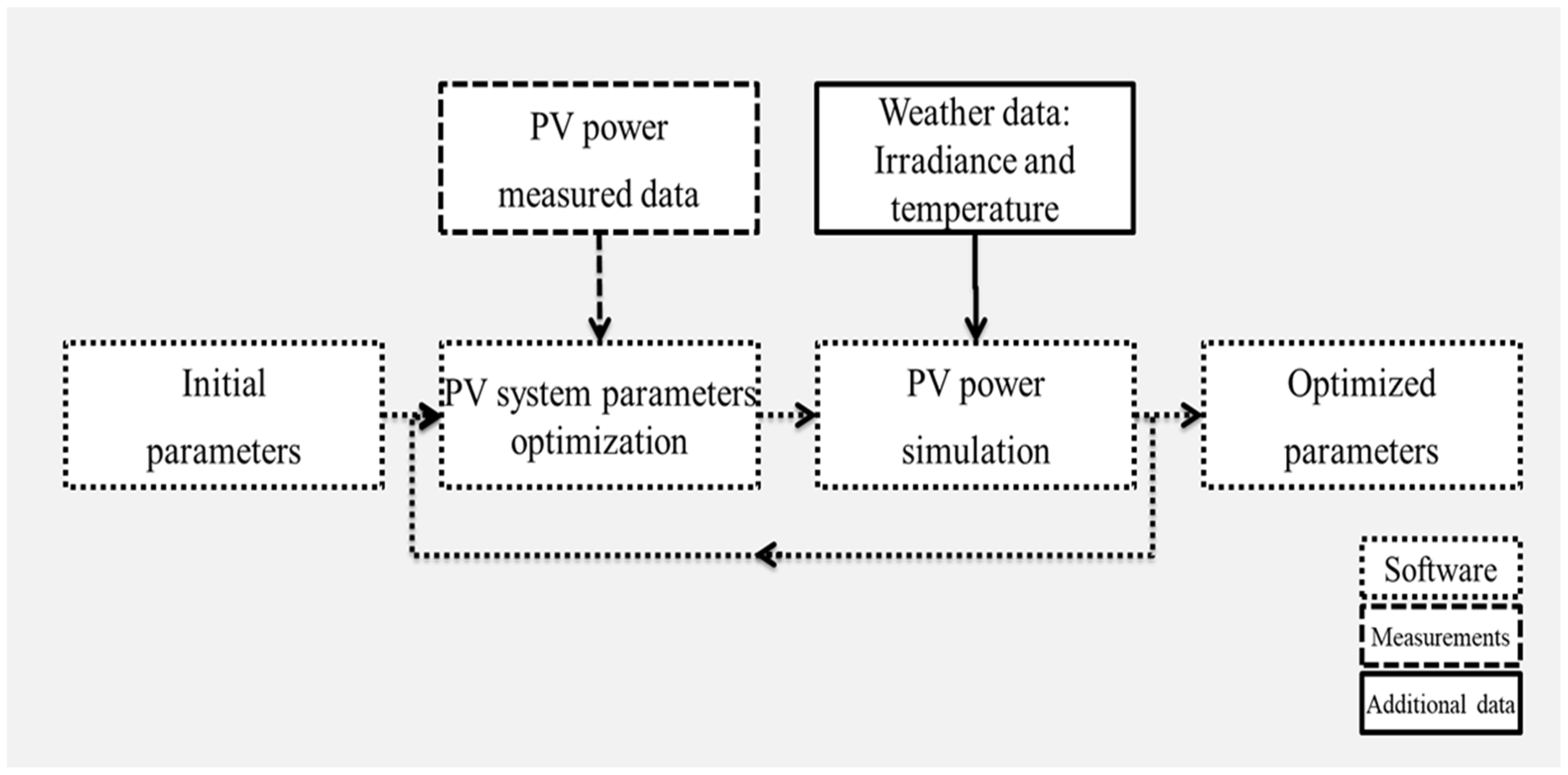
Figure 1 shows a diagram with the interactions between input data, both measured and meteorological, and processes to be performed at each phase of the methodology to optimize the PV system parameters. In this section we offer a holistic overview of each one of the methods implemented and the data used in this article.
3.1. Methods
3.1.1. PV System Simulation
In this work, we used a tested and validated chain of models that are developed and used at Fraunhofer ISE, e.g., for yield predictions [20] or energy rating [21] applications. At the current state, our algorithm, to learn and optimize parameters of an unknown PV system or subsystem, uses a slightly simplified modelling chain, and neglects some performance loss effects, i.e., soiling, degradation, internal row and surroundings shadowing, and snow. Validated models for these performance loss effects will be added to further improve the whole methodology.
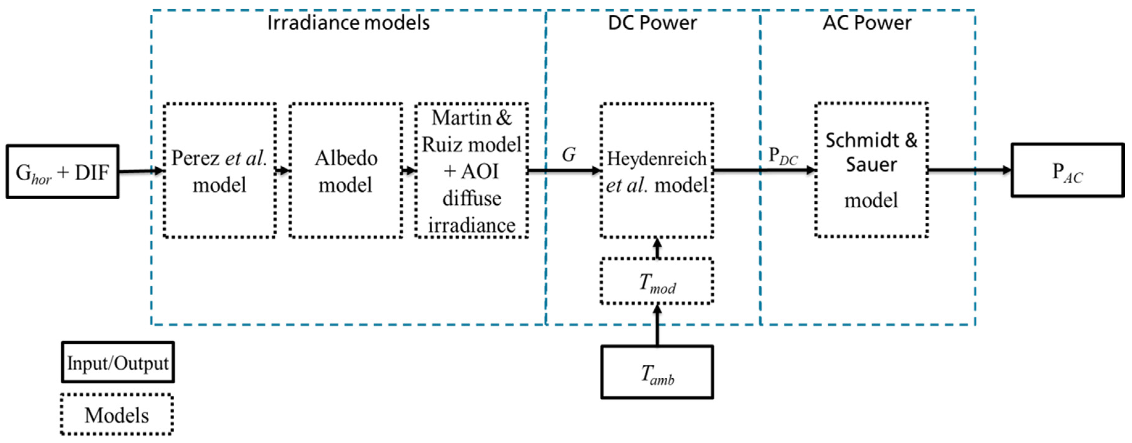
The simplified chain defined for this work consists of three main steps, described in Figure 2. In Figure 2 the main models of each step of the PV power simulation tool are described with a dotted-square, the inputs and outputs of the simulation are represented by solid-lined-squares, and finally the interaction between the models, inputs, and outputs are represented by back arrows. The three main simulation steps will be described in detail in subsections below.
Irradiance Transposition Mode, Albedo, and AOI Effect
In the first step, direct and diffuse irradiance in plane of array are calculated separately. Direct irradiance in the plane of array can be calculated straightforwardly considering the sun position at any given moment, but to calculate the diffuse part of the irradiance in the plane of array we use the model developed by Perez et al. [22].
In order to estimate the albedo produced by the surroundings in a given location, a helper function for direct irradiance in the plane of array can be used. Additional information regarding the function to estimate the albedo can be found in the original publication of the Perez model, as well as in the Klucher [23], Hay [24], and Gueymard [25] models.
To calculate the angle of incidence (AOI) effect, the Martin and Ruiz model [26] is used. The magnitude of the angle dependent losses within this modelling step depends on the position of the sun on a specific location, the tilt and azimuth angles for the specific PV module, and the ratio of direct and diffuse irradiance on the plane of array. Therefore, reflection losses are calculated separately for the direct and the diffuse irradiance on the plane of array. For direct irradiance, AOI and module reflection behavior are combined for each time-step. Whereas for diffuse irradiance, as described in [21], a generalized AOI between 50° and 60° is assumed, and 3.5% losses are assumed for all time-steps.
DC Power
In the second step, PV module temperature is calculated as suggested in [21]. An irradiance-dependent value is added to the SolarGIS ambient temperature:
where is the module temperature, is the ambient temperature, and is the irradiance in plane of array.
As [21] mentions, Equation (5) is a simplification that does not distinguish between different PV module technologies, and it excludes wind speed and direction.
After the module temperature is calculated, the PV module temperature and irradiance dependency can be calculated, as suggested by Heydenreich et al. [27]:
where is 25 °C, is the PV module efficiency at specific conditions, constants ,, and are the three parameters fitting the curve of the PV module efficiency behavior at any given irradiance, and is the temperature coefficient which describes the PV module power (or efficiency) behavior at any given temperature.
AC Power
In the last step, AC power is simulated using the same tool from previous publications [20,29,30]. Therein, some factors are considered individually, such as module mismatch, inverter efficiency, inverter power limitation, and AC cable losses.
To simulate the inverter, we use the model proposed by Schmidt and Sauer [31].
3.1.2. PV System Parameters Optimization
The GA is a process for solving complex optimization problems inspired by biological evolution. This evolutionary optimization technique was introduced first by Holland [32] in 1975, in order to search for the global optimum value of a specific problem. GA optimization is advantageous because a low amount of data is required for the optimization, objective values do not have to be known beforehand, and an absence of a gradient function simplifies the cost function definition. However, a global optimum value is not granted as a result of the optimization, even if a convex function is considered.
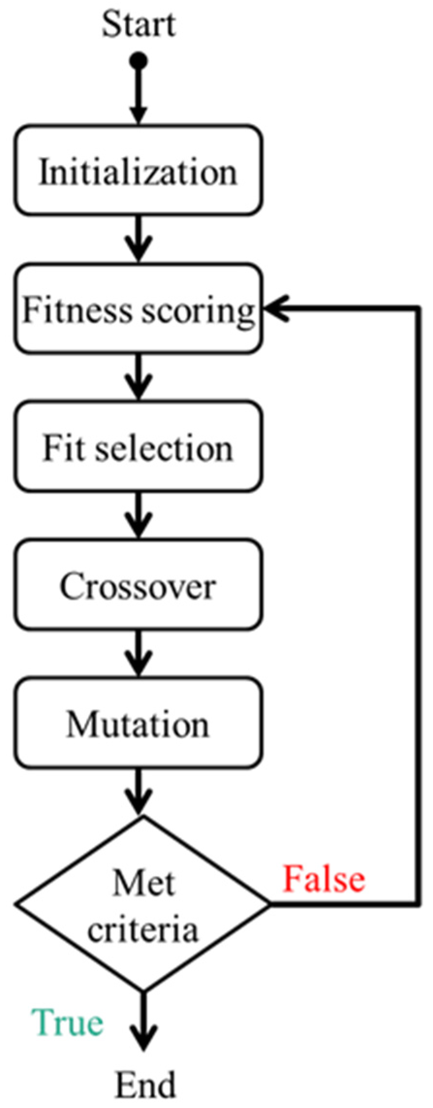
The GA proposed here relies entirely on a combination of both meteorological and PV power output measured data. We have developed an in-house GA based on the flow diagram shown in Figure 3. The GA optimization process consists of a series of six steps to follow:
- The initialization step creates a vector of different PV plants configurations (members), assigning random values (also known as population) based on the initial value to be optimized (initial parameters), with a randomness percentage defined beforehand. The PV power configuration can differ from several elements or only one.
- In the fitness scoring step, every single PV plant configuration of the population is compared with the monitoring data, evaluated, and a score is assigned based on the loss function defined.
- In the fit selection step, some PV plant configurations of the population are stochastically selected based on their scores; the higher the score, the higher the probability to be selected and passed to the next population.
- In the crossover step, some pairs of PV plant configurations resulting from the fit selection step are selected stochastically and their parameters are randomly combined. Hence, new PV plant configurations are added to the new population.
- In the mutation step, some parameters of the PV plant configurations are mutated due to a mutation probability assigned randomly to each parameter of every PV power plant configuration of the next generation.
- Finally, the next population is repopulated based on the parameters of the best PV plant configuration of the current population. The process stops when the stop criteria have been met; the stop criteria is defined in detail further in this section.
High deviations in overcast days are inherent in satellite-based meteorological data, partly due to the spatial resolution [33]. These deviations increase when satellite-based irradiance is used in combination with transposition models [20]. Considering these, we defined the cost function as the MAD between simulated and measured power (4). We minimized the cost function value by adjusting the simulation parameters with GA optimization.
We monitored two parameters from the current population along each one of the GA optimization iterations. In one instance we monitored the progress of the MAD value of the best member of the GA optimization, and in the other instance we monitored the improvement of the average MAD value of the current population.
The process is interrupted, and the criteria are met after five consecutive iterations without an improvement of both parameters; the MAD value of the best member and the mean MAD value of the current population.
The six steps of the process shown in Figure 3 are performed to learn and optimize every parameter of the PV system. The PV system parameters are optimized by comparing the measured PV power with the three different stages of the PV power simulation (see section Methods, PV system simulation) as follows:
Irradiance Transposition Mode, Albedo, and AOI Effect
In a fixed-tilt PV system, the PV power production normalized by peak power is approximately proportional to the incident irradiance [34]. Hence, we can infer that the highest incident irradiance point produces the highest power point. We normalize the PV power curve by the highest power point, and the irradiance in plane of array is normalized by the highest irradiance in plane of array.
In the first step, we optimize the albedo, tilt, and azimuth angles using GA by comparing normalized simulated irradiance in plane of array (AOI and albedo included) with normalized measured PV power.
DC Power
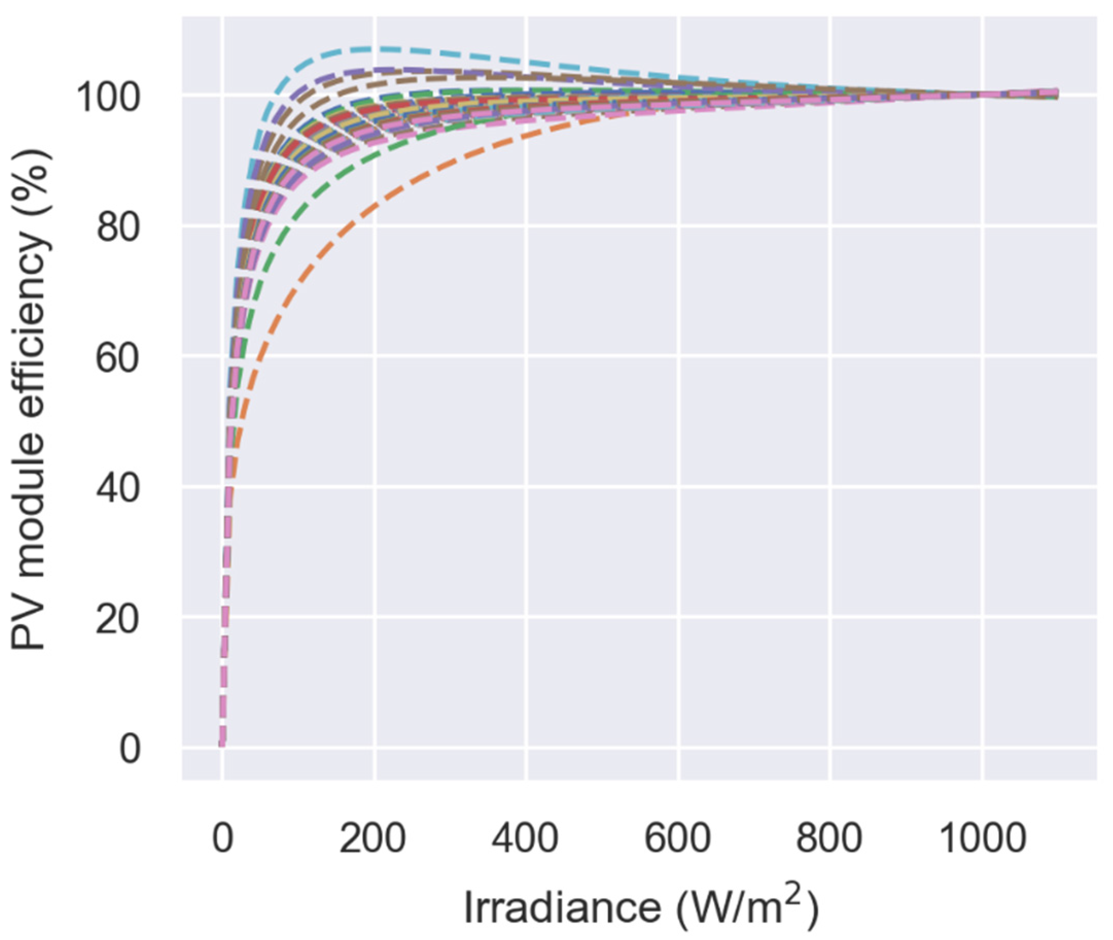
We created a database with 107 different parameters of the Heydenreich et al. model based on measurements of PV efficiency at different irradiance levels performed by Fraunhofer ISE CalLab.
In the second step, we extract the three parameters from the Heydenreich et al. model and create the database by fitting (6) for every measured curve using least squares optimization, a function available in SciPy library for Python [35]. Figure 4 shows the 107 different fitted efficiency curves, using the Heydenreich et al. model at different irradiance levels.
In order to optimize PV power DC, we propose the following two steps. First, assume an installed capacity of 1 kWp. Second, use cross validation optimization (we evaluate every set of three parameters) to select the best fit for the three parameters from the Heydenreich et al. model, and GA optimization can be used to learn the temperature coefficient.
In this step, simulated PV power DC and normalized measured PV power are compared. Simulated PV power DC is based on the direct and diffuse irradiance in the plane of array, calculated using the parameters before learning and optimizing, i.e., albedo, tilt, and azimuth angles.
AC Power
To optimize the DC to AC ratio, we assumed a 1 kWp nominal power PV system. Based on the Schmidt and Sauer model, we minimized the deviation between simulated PV power AC and normalized measured PV power using GA. PV power AC is calculated using the parameters optimized beforehand with 1% cabling losses assumed.
Finally, the nominal power is optimized with GA, comparing the simulated PV power AC with the measured PV power.
After learning and optimizing the basic parameters of a PV system or subsystem, a digital twin can be created to simulate its current or future behavior just by changing to the current or future weather conditions.
A digital twin is a digital replica of a physical PV system; this digital representation is used in this work for two main reasons: First, based on the PV parameters learned, we can create a connection between a virtual model of a PV system with a PV system modelled digitally. Second, we can change real-time weather conditions (input data) to digitally simulate (now-cast) the output power of a real PV system.
3.1.3. Clear-Sky Detection
A training data set comprised of only clear-sky-like periods can be used as an alternative to learn and optimize the basic parameters of a PV system or subsystem, and to create a digital twin. In order to identify the clear-sky-like periods, we implemented a method based on two steps:
- We used a Python function called detect_clearsky, available in PVLib library [38], to compare the statistical clear-sky curve based on measured PV power, with actual measured PV power. Hence, we were able to identify the clear-sky-like periods in the time series data set. It is important to mention that the parameters of the Python function were tuned by trial and error based on the input data, as suggested by [18].
Clear-sky-like periods are detected through a comparison between the statistical clear-sky curve and the PV power measured. Note that both the method and the python function were designed to identify clear-sky-like periods by comparing a statistical clear-sky curve based on global horizontal irradiance with the actual global horizontal irradiance.
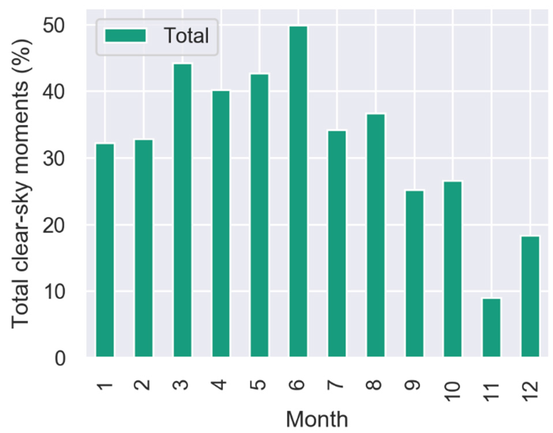
The distribution of the clear-sky-like periods of a data set from a PV system located in south-west Germany in the year 2017 is shown in Figure 5. A filter to consider PV power values only during daytime (values of global irradiance in the plane of array higher than zero) was applied to the data set.
Figure 5 shows that, on the one hand, a high density of clear-sky-like periods can be observed in spring and summer months. On the other hand, autumn and winter months have a low density of clear-sky-like periods, especially in November and December, with 9% and 18% of the total measured PV power moments, respectively.
3.2. Data Used in This Article
3.2.1. Weather Data
To simulate the AC energy yield of a PV system, a chain of different models and a time series of operating conditions (weather data) is used. We use a satellite-derived basic weather data set provided by SolarGIS [39] for the PV power simulation. More precisely, weather data from a location in south-west Germany comprises ambient temperature (), global horizontal irradiance (), and diffuse horizontal irradiance (DIF) from the year 2017 and the last 90 days of 2016, in a time series format with 15 min resolution.
3.2.2. PV Power Measured Data
The measured PV power data of the year 2017 and the last 90 days of 2016 have been collected from a real-life PV system with 5 min resolution installed on January 1st of 2010, in south-west Germany. The basic properties of the PV power plant and the parameters used as starting values for the simulation are shown in Table 1. They are extracted from different sources: tilt angle, azimuth angle, nominal power from the design layout, temperature coefficient from the PV module datasheet, and the rest of the parameters are simply assumptions. The PV parameters listed in Table 1 will be referred to as reported parameters throughout the rest of this work.
3.2.3. Initial Parameters
The initial parameters include a list of values defined for the main parameters needed to describe a general PV system or subsystem and simulate its power output. These parameters are the initial values for the optimization, to be optimized with the GA optimization process. PV system nominal power, tilt and azimuth angles, albedo, irradiance and temperature module dependency, and DC to AC ratio are included among them.
The following values have been chosen as the initial parameters for this work:
- Nominal power = 1 kWp
- Tilt angle = 25°
- Azimuth angle = 180° (south oriented)
- Albedo = 0.2
- Temperature coefficient = −0.43%/°C
- DC to AC ratio = 1
It has been found with the optimizations performed throughout this work that the values of the initial parameters have no direct relation with the final result, yet they can reduce the total computational time.
4. Results and Discussion
To fully cover seasonality effects and at the same time limit the computation time needed, we applied the GA algorithm to one day per week of the year 2017. After a day has been selected, we used three different training data sets comprised of 30, 60, and 90 all-sky days before the selected day. These three different training periods should provide a first impression on the impact of the length of the training period on parametrization and now-casting accuracy. As a product of the PV system parameters optimization, a digital twin is created for each of the training data sets.
Next, we evaluated the accuracy of the digital twin of the selected day by comparing daytime values of measured PV power with the digital twin simulated PV power. In order to translate the accuracy of the GA optimization proposed within this work to any given PV system or subsystem, the MBD is given in W/kWp.
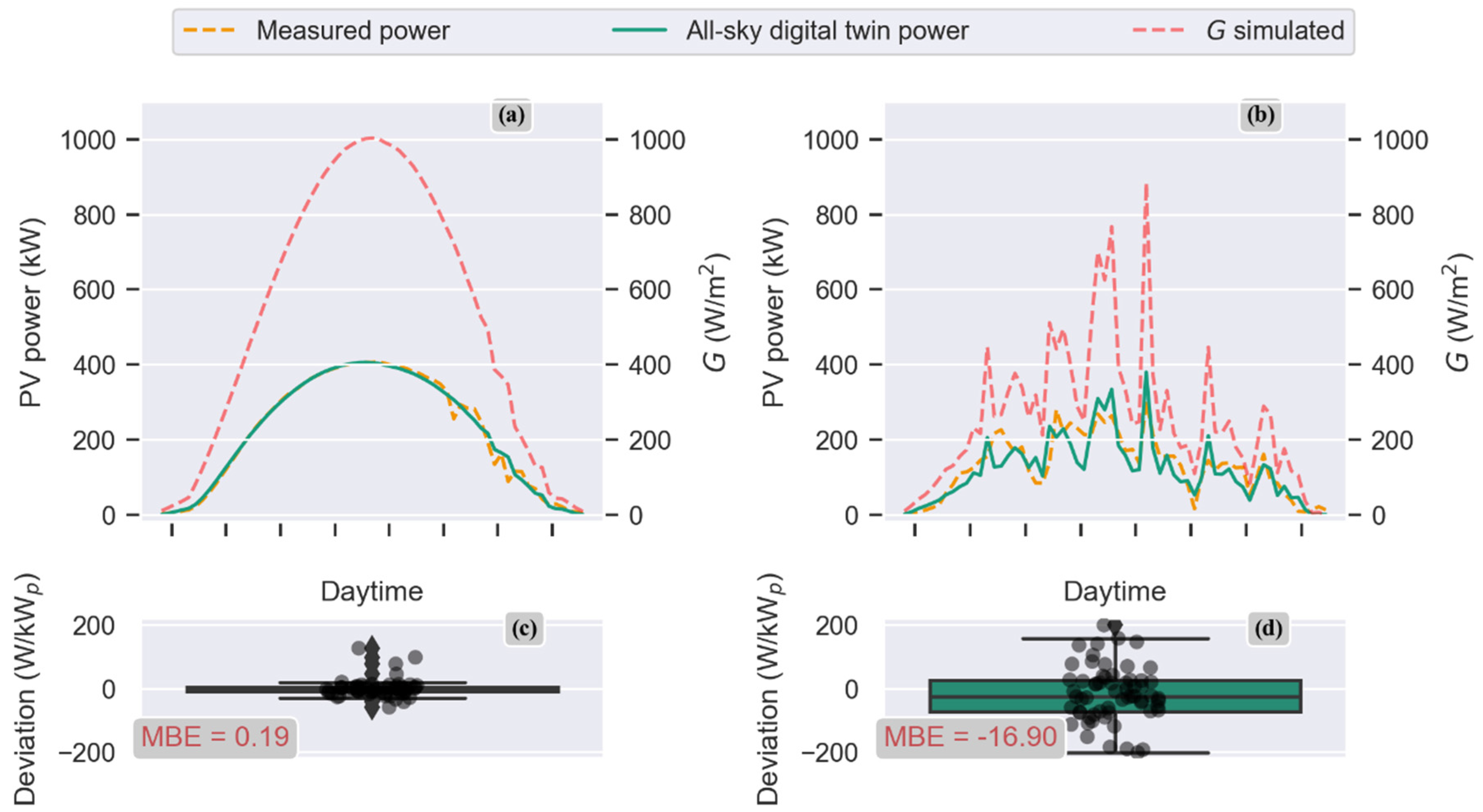
The PV power simulated with two digital twins, optimized with 30 days of all-sky training data, and measured PV power of a clear-sky and an overcast day of 2017, are exemplified in Figure 6. Figure 6a,b show the PV power measured, the PV power simulated with the digital twin, and the simulated irradiance in the plane of array. Figure 6c,d show the deviation between the digital twin and PV power measured. It is evident that higher deviations are presented in overcast conditions.
Figure 6a,b show the mean deviation between daytime PV power measurements and the digital twin simulated PV power values equal to 0.19 W/kWp and −16.90 W/kWp, respectively. Only daytime values are considered in both examples.
In a similar fashion, data sets comprised of only clear-sky-like periods can be used to train and create a new set of parameters comprising a new digital twin. Like the all-sky conditions training phase, three different lengths for training data sets were used to optimize the PV system parameters with only clear-sky-like periods, create a digital twin, and evaluate the now-casting accuracy.
In the first part of this section, we present a detailed description of the results of the PV system parametrization, considering all-sky and clear-sky conditions within the training data sets. In the second part of this section, we compare the accuracy of digital twins generated considering all-sky and clear-sky conditions.
4.1. PV System Parametrization
Table 2 comprises a quantitative analysis for all the PV system parameters optimization of the 52 days considering both, clear-day and all-sky situations, and the three different lengths for the training data sets.
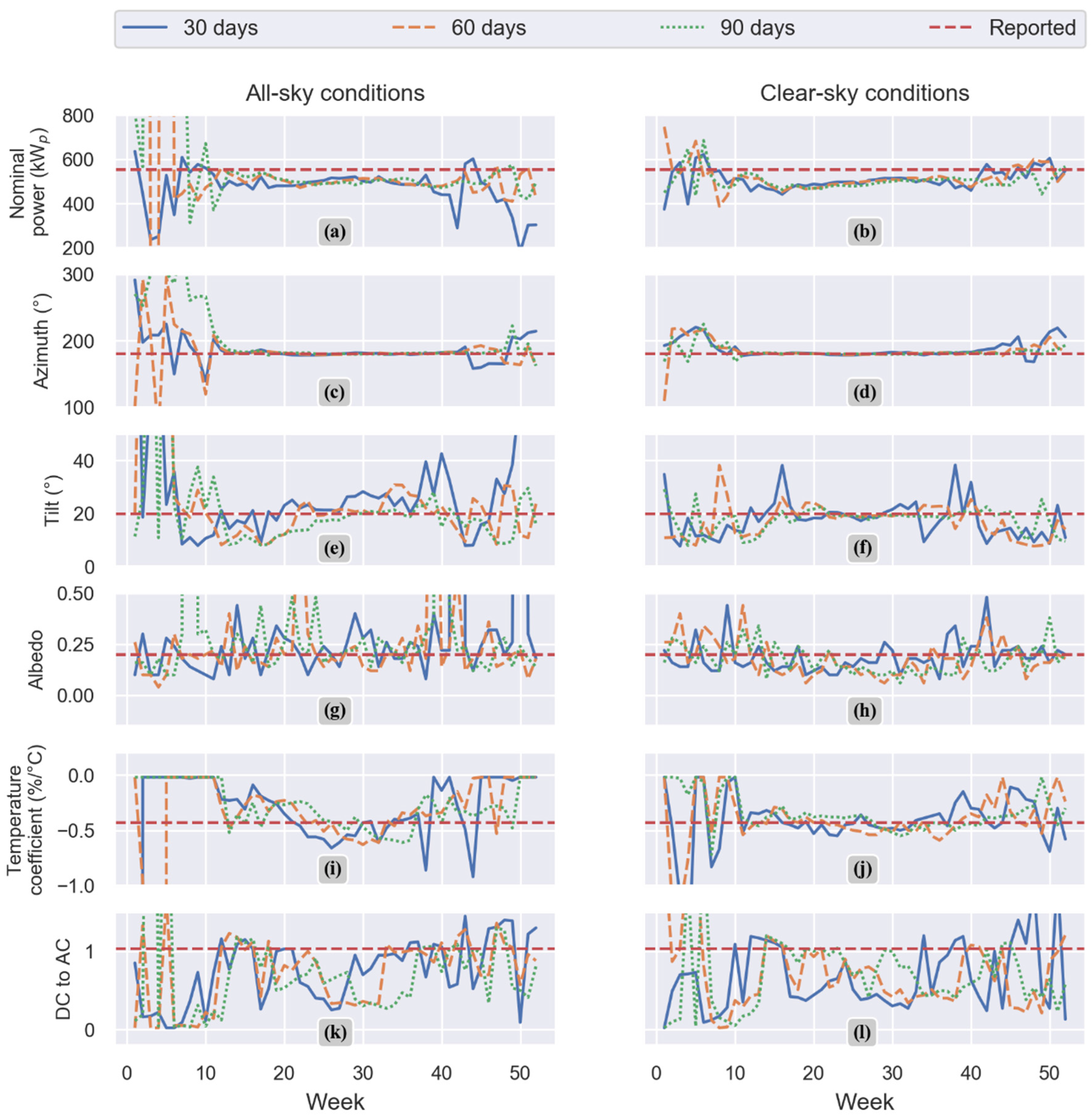
Figure 7 shows plots for every optimized parameter of 52 chosen days, comparing different training set lengths: 30 days, 60 days, 90 days, and the reported parameter. An additional comparison between all-sky and clear-sky conditions is also presented. Thirty days is represented by the blue solid line, 60 days is represented by the orange dashed-line, 90 days is represented by a green dotted-line, and the reported parameter is represented by a horizontal red dashed-line.
On the left-hand side of Figure 7, the results for the optimized parameters considering all-sky conditions within the training data sets are shown, and the results for the optimized parameters considering only clear-sky conditions within the training data sets can be observed on the right hand side of Figure 7.
According to [40], PV power output is almost linearly correlated to the incident irradiance on the plane of array. Moreover, according to [41], deviations on satellite-based solar irradiance data have a general correlation with the number of overcast days. Hence, a higher deviation on simulated PV power is expected as a result of overcast situations, which consequently cause high variability on the parametrization process. This effect can be observed in all the subplots of Figure 7, particularly in months with less clear-sky-like periods (see Figure 5). Opposite to this effect, a better agreement between the optimized and the reported parameters can be observed during months with a higher number of clear-sky-like periods.
A possible reason for the huge overestimation of nominal power at the beginning of the year 2017 may be due to snow: while the ground is covered by snow, the irradiance algorithm may interpret the relatively bright pixels as clouds, and as a consequence will assume overcast conditions and calculate drastically underestimated irradiance values [42]. When the snow on the PV system is melted or removed, the measured absolute power as input for the GA optimization will be high compared to the irradiance. The GA algorithm will compensate for this effect by an increase of the nominal power. The overall error metrics in Table 2 are influenced by the high absolute deviations in these situations. A strong influence on the error metrics for all other parameters is likely, mostly when all-sky conditions are used as training data.
An alternative to reduce the very high variability of the optimized parameters at winter season, and when all-sky conditions are used as training data, is to add physical limitations to the optimized parameters, e.g., extremely high (physically impossible) albedo, tilt angles, and DC to AC ratio values can be limited within the GA algorithm, as well as extremely low temperature coefficients. Additionally, an error can be reported instead of those nonmeaningful values.
The parametrization results of nominal power are shown in Figure 7a,b. It is evident that in both plots the optimization process results in an underestimation of the nominal power. Figure 7a shows high variability in months with fewer clear-sky-like periods for the three lengths of the training data sets. As Table 2 describes, a training data set of 30 days before is enough to achieve a MBD of −84.24 kWp, which is equal to −18% of the reported installed capacity. Figure 7b shows less variability in general, with an MAPD of 10.69% for the worst-case scenario using a training data set of 90 days before. It shows that, it is possible to achieve a mean deviation of less than 10% of the reported installed capacity using clear-sky-like periods as training data.
According to [43], a mean degradation rate of 0.8% to 0.9% per year can be expected for PV power plants. Since the PV system under study was installed in 2010, the deviation in nominal power can be explained partly by an expected degradation factor. However, as mentioned in [44], the total PV power of a PV plant can be affected by additional loss mechanisms, including loss effects such as long-term soiling, which can be reversible (see week 20 to 52 of Figure 7b).
Azimuth angle optimization results can be observed in Figure 7c,d. Although slightly overestimated, both subplots show a good agreement between the results of the three data set lengths and the reported value, with a higher deviation in the months with fewer clear-sky-like periods, particularly when all-sky conditions are considered. Benchmark publications [17,18,19] have reported a deviation of between 4° and 5° for the azimuth angle parametrization. In this work, we show a mean deviation of less than 3° with a training data set of 90 days with only clear-sky-like periods.
Results of tilt angle optimization considering all-sky and clear-sky conditions are shown in Figure 7e,f, respectively. Deviation values reported by [17,19], between 2° and 2.55°, show a good agreement with the results of this work, mostly when only clear-sky-like periods are considered as training data set.
The results of the albedo optimization are shown in Figure 7g for all-sky conditions and Figure 7h for clear-sky conditions. Albedo ground reflection factor has been reported as 0.2, similar to the value proposed by [45]. However, both subplots present high variability, which can be explained by [46,47], where it is concluded that a constant value for an albedo is unrealistic.
As suggested by [48], albedo has a strong seasonal dependency. Figure 7h shows a seasonal variation with lower values in summer months and higher values in winter months. Within this work, albedo is underestimated when 90 days of clear-sky-like periods are considered for the training data with a MBD of −0.02.
As observed in subplots (i,j) of Figure 7, temperature coefficient optimization results show higher relative variability when compared with the rest of the parameters, especially in winter months. This can be explained by the low temperatures during such months. When only clear-sky conditions are considered as training data sets for the optimization, using GA is possible to achieve a mean deviation between 0.01%/C and 0.09%/C.
DC to AC ratio optimization results are shown in subplots (k,l) of Figure 7. The GA proposed here achieved an MBD of −0.14, with a training data set comprised of 90 days before, and all-sky conditions, and an MBD of −0.35 with 90 days of clear-sky-like moments as training data set.
Table 3 contains the optimized parameters for the Heydenreich et al. model. On the one hand, the three parameters for the PV simulation trained only with all-sky conditions, and on the other hand, the three parameters for the PV simulation trained only with clear-sky days.
In general, Figure 7 and Table 2 show a better agreement between the optimized parameters and the reported ones when only clear-sky-like periods are considered. Furthermore, it is shown that, in general, quality and length of the training data is of high importance, shorter training data sets can include seasonality effects, and these can be reflected in the optimization process. Moreover, an increment on the size of the training data set seems to improve the results of the GA optimization.
According to Figure 7 and Table 2, and specifically for the PV system analyzed in this work, one can assume the following constraints were the best conditions for the parametrization process for this particular PV system (the number of clear-sky-like periods can differ depending on the geographical location) combined with satellite-based irradiance data: 90 days of training data and better results are achieved within the course of 10 weeks—from week 20 to week 30 of the year 2017.
Table 4 contains a comparison between the reported parameters and the parameters optimized considering the best conditions defined above. As shown in Table 4, when considering only the best conditions for the GA optimization of this particular PV system, the absolute deviation between reported values and the MBD of the optimized values is considerably lower. Specifically, parameters such as tilt angle, with an absolute deviation of 0.4°, azimuth angle, with an absolute deviation of 0.76°, temperature coefficient, with an absolute deviation of 0.02%/°C, and an absolute deviation of 35.2 kWp, when a loss factor of 0.8%/year for the nominal power is considered.
4.2. Digital Twin Now-Casting
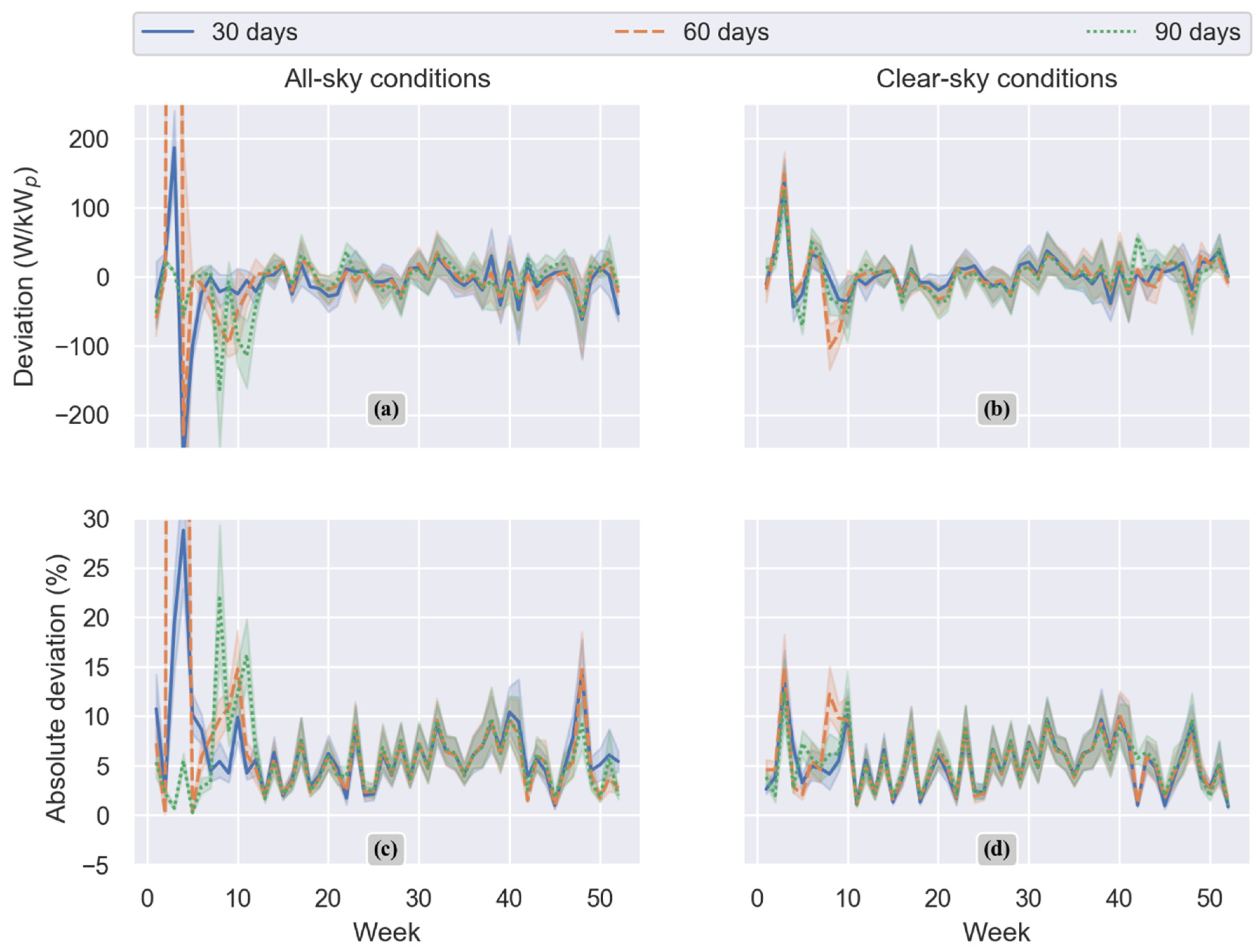
Although the optimized parameters throughout the year show some variation, this variation is not directly correlated with the accuracy of the digital twin PV power now-casting when compared with the actual PV power measured.
Figure 8 illustrates the deviation between the digital twin PV power simulated and the measured power throughout daytime of 52 days of year 2017. Figure 8a,c show the deviation and absolute deviation in percentage when all-sky conditions are considered within the training data set to create the digital twin. As it can be observed, subplots (a,c) show higher deviation and absolute deviation during the first 11 weeks, specifically when the training sets are 30 and 60 days length.
Table 5 contains the deviation results of the comparison between the digital twin simulated PV power and the measured PV power from 52 randomly chosen days in the year 2017. The table describes in detail the accuracy of the digital twins depending on the sky conditions (all-sky and clear-sky) and the training data set lengths.
In Figure 8b,d, and in Table 5, it can be observed that digital twins created with only clear-sky training data perform more accurately than the ones considering all-sky conditions. Like the parametrization results, an increment of on the length of the training data set will improve the overall performance of the digital twin.
The GA optimization proposed here shows that if only clear-sky-like periods are considered for the training of the digital twin, an MBD between −0.39 W/kWp and 1.53 W/kWp is feasible. Using the GA proposed here, based on satellite-derived weather data, we can now-cast the PV power of a PV system with higher accuracy than previous publications with a MAPD lower than 6%, without evident seasonal effects. MAPD values above 10% have been reported for previous publications by [4,5,6,7,8].
4.3. Limitations
It is important to mention that the GA optimization method proposed here also has some limitations. Firstly, throughout the PV power simulation and the optimization processes, the deviation between satellite-based irradiance data and on-site measured irradiance data have been neglected, as well as some performance loss effects such as horizon or surrounding shading, internal row shading, dust and soiling, snow, and degradation. Secondly, this GA optimization method was not tested to optimize parameters and now-cast a bifacial PV system nor single or multiple axis tracked PV systems.
Furthermore, the GA can produce physically nonmeaningful parameters due to the lack of physical limits within the optimization process, mostly when all-sky conditions are used as training data.
4.4. Future Directions
The GA proposed here can be used as an interesting key performance index (KPI) generator for operation and maintenance of PV systems. Based on the current work, a longer training data set may lead to a more accurate now-casting and more stable parametrization results. Extraction of performance loss effects, such as degradation or soiling, can be possible by parametrizing a PV system with longer training data sets and monitoring the behavior of some PV parameters, i.e., nominal power and DC to AC ratio. Furthermore, real-time malfunctions of a PV system can be detected by a comparison between the PV power simulated by the digital twin and the PV power measured on-site.
Additionally, it can be set that warnings or errors are reported instead of physically nonmeaningful parameters, or physical limits can be set throughout the parameters optimization process in order to avoid physically nonmeaningful results.
Finally, the deviations in both PV system parametrization and digital twin now-casting can be reduced by using on-site measured weather data. As a continuation of this publication, the publication of a second part is planned that only uses on-site measured weather data and PV power output, considering longer training sets for the GA and digital twinning.
5. Conclusions
A GA approach was proposed in this work to learn and optimize seven PV parameters of an unknown PV system or subsystem, create a digital twin, and now-cast the PV power based on satellite-based weather data and measured PV power. It is evident that the GA approach suggested here performs better when only clear-sky-like periods are considered as training data.
By using the GA approach proposed in this work to parametrize a PV system or subsystem, it has been shown that the following can be achieved: a MBD of less than 10% for the nominal power, a MBD of less than 3° for azimuth angle, a MBD of less than 3° for tilt angle, and a MBD between 0.01%/C and 0.09%/C for the temperature coefficient. A significant deviation reduction on the PV parametrization is possible if the best conditions for the GA optimizations are defined for a specific PV system and if access to larger training data sets is granted.
A MAPD of less than 6% and an MBD of about −0.39 W/kWp have been estimated for the digital twin now-casting accuracy of the GA approach of this work.
Additional on-site meteorological and environmental measurements for the systems under consideration would be beneficial to increase the overall performance of the GA algorithm and digital twin.
Author Contributions
Conceptualization, data processing, simulations, and analyses, D.E.G.R. and B.M., H.M., and C.W. discussed the results and improved the overall results of this publication. All authors have read and agreed to the published version of the manuscript.
Funding
The authors acknowledge the financial support by the Federal Ministry for Economic Affairs and Energy of Germany (BMWi) in the project ALPRO (project number 0324054A).
Conflicts of Interest
The authors declare no conflict of interest.
References
- International Energy Agency. Trends in Photovoltaic Applications; Technical Report No. IEA PVPS T1-36; International Energy Agency: Paris, France, 2019. [Google Scholar]
- Wood Mackenzie. Ami Global Forecast 2019–2024; Technical Report No. H1 2019; Wood Mackenzie: Edinburgh, UK, 2020. [Google Scholar]
- Mellit, A.; Kalogirou, S.A. Artificial intelligence techniques for photovoltaic applications: A review. Prog. Energy Combust. Sci. 2008, 34, 574–632. [Google Scholar] [CrossRef]
- Ding, M.; Wang, L.; Bi, R. An ANN-based approach for forecasting the power output of photovoltaic system. Proc. Environ. Sci. 2011, 11, 1308–1315. [Google Scholar] [CrossRef] [Green Version]
- Mandal, P.; Madhira, S.T.S.; Haque, A.U.; Meng, J.; Pineda, R.L. Forecasting power output of solar photovoltaic system using wavelet transform and artificial intelligence techniques. Proc. Comput. Sci. 2012, 12, 332–337. [Google Scholar] [CrossRef] [Green Version]
- Ibrahim, I.A.; Mohamed, A.; Khatib, T. Modeling of photovoltaic array using random forests technique. In Proceedings of the IEEE Conference on Energy Conversion, Johor Bahru, Malaysia, 19–20 October 2015. [Google Scholar]
- Landelius, T.; Andersson, S.; Abrahamsson, R. Modelling and forecasting PV production in the absence of behind-the-meter measurements. Prog. Photovolt Res. Appl. 2019, 27, 990–998. [Google Scholar] [CrossRef] [Green Version]
- Monteiro, C.; Fernandez-Jimenez, L.A.; Ramirez-Rosado, I.J.; Muñoz-Jimenez, A.; Lara-Santillan, P.M. Short-term forecasting models for photovoltaic plants: Analytical vs. soft-computing techniques. Math. Probl. Eng. 2013, 2013, 767284. [Google Scholar] [CrossRef] [Green Version]
- Yona, A.; Senjyu, T.; Saber, A.Y.; Funabashi, T.; Sekine, H.; Kim, C.H. Application of neural network to 24-hour-ahead generating power forecasting for PV system. In Proceedings of the 2008 IEEE Power and Energy Society General Meeting, Pittsburgh, PA, USA, 20–24 July 2008. [Google Scholar]
- Da Silva Fonseca, J.G.; Oozeki, T.; Takashima, T.; Koshimizu, G.; Uchida, Y.; Ogimoto, K. Use of support vector regression and numerically predicted cloudiness to forecast power output of a photovoltaic power plant in Kitakyushu, Japan. Prog. Photovolt: Res. Appl. 2012, 20, 874–882. [Google Scholar] [CrossRef]
- Dolara, A.; Grimaccia, F.; Leva, S.; Mussetta, M.; Ogliari, E. A physical hybrid artificial neural network for short term forecasting of pv plant power output. Energies 2015, 8, 1138. [Google Scholar] [CrossRef] [Green Version]
- Muhsen, D.H.; Ghazali, A.B.; Khatib, T.; Abed, I.A. A comparative study of evolutionary algorithms and adapting control parameters for estimating the parameters of a single-diode photovoltaic module’s model. Renew. Energy 2016, 96, 377–389. [Google Scholar] [CrossRef]
- Ma, J.; Bi, Z.; Ting, T.O.; Hao, S.; Hao, W. Comparative performance on photovoltaic model parameter identification via bio-inspired algorithms. Sol. Energy 2016, 132, 606–616. [Google Scholar] [CrossRef]
- Kichou, S.; Silvestre, S.; Guglielminotti, L.; Mora-López, L.; Muñoz-Cerón, E. Comparison of two PV array models for the simulation of PV systems using five different algorithms for the parameters identification. Renew. Energy 2016, 99, 270–279. [Google Scholar] [CrossRef]
- Bastidas-Rodriguez, J.D.; Petrone, G.; Ramos-Paja, C.A.; Spagnuolo, G. A genetic algorithm for identifying the single diode model parameters of a photovoltaic panel. Math. Comput. Simul. 2017, 131, 38–54. [Google Scholar] [CrossRef]
- Ismail, M.S.; Moghavvemi, M.; Mahlia, T.M.I. Characterization of PV panel and global optimization of its model parameters using genetic algorithm. Energy Convers. Manag. 2013, 73, 10–25. [Google Scholar] [CrossRef]
- Saint-Drenan, Y.M.; Bofinger, S.; Fritz, R.; Vogt, S.; Good, G.H.; Dobschinski, J. An empirical approach to parameterizing photovoltaic plants for power forecasting and simulation. Sol. Energy 2015, 120, 479–493. [Google Scholar] [CrossRef] [Green Version]
- Killinger, S.; Engerer, N.; Müller, B. QCPV: A quality control algorithm for distributed photovoltaic array power output. Sol. Energy 2017, 143, 120–131. [Google Scholar] [CrossRef]
- Mason, K.; Reno, M.J.; Blakely, L.; Vejdan, S.; Grijalva, S. A deep neural network approach for behind-the-meter residential PV size, tilt and azimuth estimation. Sol. Energy 2020, 196, 260–269. [Google Scholar] [CrossRef]
- Müller, B.; Hardt, L.; Armbruster, A.; Kiefer, K.; Reise, C. Yield predictions for photovoltaic power plants: Empirical validation, recent advances and remaining uncertainties. Prog. Photovolt Res. Appl. 2016, 24, 570–583. [Google Scholar] [CrossRef]
- Dirnberger, D.; Müller, B.; Reise, C. PV module energy rating: Opportunities and limitations. Prog. Photovolt Res. Appl. 2015, 23, 1754–1770. [Google Scholar] [CrossRef]
- Perez, R.; Ineichen, P.; Seals, R.; Michalsky, J.; Stewart, R. Modeling daylight availability and irradiance components from direct and global irradiance. Sol. Energy 1990, 44, 271–289. [Google Scholar] [CrossRef] [Green Version]
- Klucher, T.M. Evaluation of models to predict insolation on tilted surfaces. Sol. Energy 1979, 23, 111–114. [Google Scholar] [CrossRef]
- Hay, J.E. Calculation of monthly mean solar radiation for horizontal and inclined surfaces. Sol. Energy 1979, 23, 301–307. [Google Scholar] [CrossRef]
- Gueymard, C. An anisotropic solar irradiance model for tilted surfaces and its comparison with selected engineering algorithms. Sol. Energy 1987, 38, 367–386. [Google Scholar] [CrossRef]
- Martín, N.; Ruiz, J.M. A new model for PV modules angular losses under field conditions. Int. J. Sol. Energy 2002, 22, 19–31. [Google Scholar] [CrossRef]
- Heydenreich, W.; Müller, B.; Reise, C. Describing the world with three parameters: A new approach to PV module power modelling. In Proceedings of the 23rd European Photovoltaic Solar Energy Conference and Exhibition, Valencia, Spain, 1–5 September 2008; pp. 2786–2789. [Google Scholar]
- Müller, B.; Kräling, U.; Heydenreich, W.; Reise, C.; Kiefer, K. Simulation of irradiation and temperature dependent efficiency of thin film and crystalline silicon modules based on different parameterization. In Proceedings of the 5th World Conference on Photovoltaic Energy Conversion, Valencia, Spain, 6–10 September 2010; pp. 4240–4243. [Google Scholar]
- Müller, B.; Heydenreich, W.; Kiefer, K.; Reise, C. More Insights from the monitoring of real world PV power plants—A comparison of measured to predicted performance of PV systems. In Proceedings of the 24th European Photovoltaic Solar Energy Conference, Hamburg, Germany, 21–25 September 2009; pp. 3888–3892. [Google Scholar]
- Müller, B.; Reise, C.; Heydenreich, W.; Kiefer, K. Are Yield Certificates Reliable? A Comparison to Monitored Real World Results. In Proceedings of the 22nd European Photovoltaic Solar Energy Conference and Exhibition, Milano, Italy, 3–7 September 2007. [Google Scholar]
- Schmidt, H.; Sauer, D. Wechselrichter-wirkungsgrade—Praxisgerechte modellierung und abschätzung. Sonnenenergie 1994, 1996, 154. [Google Scholar]
- Holland, J.H. Adaptation in Natural and Artificial Systems. An Introductory Analysis with Applications to Biology, Control, and Artificial Intelligence; University of Michigan Press: Ann Arbor, MI, USA, 1975; ISBN 0472084607. [Google Scholar]
- Lorenz, E.; Hurka, J.; Heinemann, D.; Beyer, H.G. Irradiance Forecasting for the Power Prediction of Grid-Connected Photovoltaic Systems. IEEE J. Sel. Top. Appl. Earth Obs. Remote Sens. 2009, 2, 2–10. [Google Scholar] [CrossRef]
- Lonij, V.P.A.; Jayadevan, V.T.; Brooks, A.E.; Rodriguez, J.J.; Koch, K.; Leuthold, M.; Cronin, A.D. Forecasts of PV power output using power measurements of 80 residential PV installs. In Proceedings of the 2012 38th IEEE Photovoltaic Specialists Conference, Austin, TX, USA, 3–8 June 2012. [Google Scholar]
- Virtanen, P.; Gommers, R.; Oliphant, T.E.; Haberland, M.; Reddy, T.; Cournapeau, D.; Burovski, E.; Peterson, P.; Weckesser, W.; Bright, J.; et al. SciPy 1.0: Fundamental algorithms for scientific computing in Python. Nat. Methods 2020, 17, 261–272. [Google Scholar] [CrossRef] [Green Version]
- Reno, M.J.; Hansen, C.W. Identification of periods of clear sky irradiance in time series of GHI measurements. Renew. Energy 2016, 90, 520–531. [Google Scholar] [CrossRef] [Green Version]
- Stein, J.S.; Hansen, C.W.; Reno, M.J. Global Horizontal Irradiance Clear Sky Models: Implementation and Analysis; Technical Report No. 2012–2389; Sandia National Labaratories: Albuquerque, NM, USA, 2012. [Google Scholar]
- Holmgren, W.; Calama-Consulting; Lorenzo, T.; Hansen, C.; Mikofski, M.; Krien, U.; Bmu; DaCoEx; Driesse, A.; Konstant_t; et al. Pvlib/Pvlib-Python, v0.7.1; Zenodo; 2020. [Google Scholar]
- Suri, M.; Cebecauer, T.; Skoczek, A. SolarGIS: Solar data and online applications for PV planning and performance assessment. In Proceedings of the 26th European Photovoltaic Solar Energy Conference and Exhibition, Hamburg, Germany, 5–9 September 2011; pp. 3930–3934. [Google Scholar]
- Louwen, A.; de Waal, A.C.; Schropp, R.E.I.; Faaij, A.P.C.; van Sark, W.G.J.H.M. Comprehensive characterisation and analysis of PV module performance under real operating conditions. Prog. Photovolt Res. Appl. 2017, 25, 218–232. [Google Scholar] [CrossRef]
- Ernst, M.; Thomson, A.; Haedrich, I.; Blakers, A. Comparison of Ground-based and Satellite-based Irradiance Data for Photovoltaic Yield Estimation. Energy Proc. 2016, 92, 546–553. [Google Scholar] [CrossRef] [Green Version]
- Dürr, B.; Zelenka, A. Deriving surface global irradiance over the Alpine region from METEOSAT Second Generation data by supplementing the HELIOSAT method. Int. J. Remote Sens. 2009, 30, 5821–5841. [Google Scholar] [CrossRef]
- Jordan, D.C.; Kurtz, S.R.; VanSant, K.; Newmiller, J. Compendium of photovoltaic degradation rates. Prog. Photovolt Res. Appl. 2016, 24, 978–989. [Google Scholar] [CrossRef]
- Kiefer, K.; Farnung, B.; Müller, B.; Reinartz, K.; Rauschen, I.; Klünter, C. Degradation in PV power plants: Theory and practice. In Proceedings of the 36th European Photovoltaic Solar Energy Conference and Exhibition, Marseille, France, 9–13 September 2018; pp. 1331–1335. [Google Scholar]
- Liu, B.Y.H.; Jordan, R.C. The long-term average performance of flat-plate solar-energy collectors. Sol. Energy 1963, 7, 53–74. [Google Scholar] [CrossRef]
- Ineichen, P.; Guisan, O.; Perez, R. Ground-reflected radiation and albedo. Sol. Energy 1990, 44, 207–214. [Google Scholar] [CrossRef] [Green Version]
- Ineichen, P.; Perez, R.; Seals, R. The importance of correct albedo determination for adequately modeling energy received by tilted surfaces. Sol. Energy 1987, 39, 301–305. [Google Scholar] [CrossRef] [Green Version]
- Iqbal, M. Ground Albedo: An Introduction to Solar Radiation; Elsevier: Amsterdam, The Netherlands, 1983; pp. 281–293. ISBN 9780123737502. [Google Scholar]
Figure 1.
General methodology for the Photovoltaic (PV) system parameters optimization. Small dotted lines represent the interactions between the software blocks. Large dotted lines represent measured PV power data as input. Continuous lines represent additional data required as input, namely meteorological data.

Figure 2.
PV power simulation model chain steps.

Figure 3.
Six step flow diagram of the genetic algorithm.

Figure 4.
Heydenreich et al. model fitted curves of 107 different Fraunhofer CalLab measurement results for module efficiency at different irradiance levels.
Figure 4.
Heydenreich et al. model fitted curves of 107 different Fraunhofer CalLab measurement results for module efficiency at different irradiance levels.

Figure 5.
Monthly distribution of clear-sky moments from a PV system located in south-west Germany in the year 2017.
Figure 5.
Monthly distribution of clear-sky moments from a PV system located in south-west Germany in the year 2017.

Figure 6.
Exemplary results of a clear-sky day (a) and an overcast day (b) of 2017 digital twin PV power simulation trained with the 30 days before. Deviations between simulated PV power and measured PV power of a clear-sky day and an overcast day are shown in subfigures (c,d), respectively.
Figure 6.
Exemplary results of a clear-sky day (a) and an overcast day (b) of 2017 digital twin PV power simulation trained with the 30 days before. Deviations between simulated PV power and measured PV power of a clear-sky day and an overcast day are shown in subfigures (c,d), respectively.

Figure 7.
Parametrization results of the GA optimization. Left hand side subfigures (a,c,e,g,i,k) show the parametrization results considering all-sky conditions as training data and right hand side subfigures (b,d,f,h,j,l) show the parametrization results considering only clear-sky conditions as training data.

Figure 8.
Digital twin now-casting results based on GA optimization. 52 chosen days of year 2017. Six different training data sets for each day were considered: all-sky and clear-sky conditions with 30, 60, and 90 days of training data sets. The lines represent the mean value and the shadows show a confidence interval of 95%, only daytime values are considered.


Table 1.
Basic reported parameters from the PV plant located in south-west Germany.
| Parameter | Value |
|---|---|
| Tilt angle (°) | 20 |
| Azimuth angle (°) | 181 |
| Albedo | 0.2 |
| Temperature coefficient (%/°C) | −0.43 |
| Heydenreich a | 0.001084 |
| Heydenreich b | −7.247061 |
| Heydenreich c | −156.5457 |
| DC to AC ratio | 1.04 |
| Nominal power (kWp) | 553 |
Table 2.
Parametrization results of the genetic algorithm (GA) optimization including all-sky and clear-sky conditions.
Table 2.
Parametrization results of the genetic algorithm (GA) optimization including all-sky and clear-sky conditions.
| Training Data Set Length | |||||||
|---|---|---|---|---|---|---|---|
| Parameter | Error Metric | All-Sky Conditions | Clear-Sky Conditions | ||||
| 30 Days | 60 Days | 90 Days | 30 Days | 60 Days | 90 Days | ||
| Nominal Power | Reported (kWp) | 553 | 553 | ||||
| Mean (kWp) | 468.76 | 890.13 | 954.05 | 509.19 | 517.5 | 503.17 | |
| MBD (kWp) | −84.24 | 337.13 | 401.05 | −43.81 | −35.5 | −49.83 | |
| MAPD (%) | 16.94 | 88.14 | 90.73 | 9.92 | 9.95 | 10.69 | |
| RMSD (kWp) | 125.46 | 2073.5 | 1995.17 | 64.33 | 66.2 | 65.31 | |
| Azimuth | Reported (°) | 181 | 181 | ||||
| Mean (°) | 185.79 | 183.09 | 204.09 | 187.37 | 185.06 | 183.47 | |
| MBD (°) | 4.79 | 2.09 | 23.09 | 6.37 | 4.06 | 2.47 | |
| MAPD (%) | 6.63 | 8.55 | 13.51 | 4.58 | 4.24 | 2.53 | |
| RMSD (°) | 22.18 | 33.43 | 50.81 | 13.91 | 15.79 | 9.3 | |
| Tilt | Reported (°) | 20 | 20 | ||||
| Mean (°) | 29.06 | 29.95 | 22.65 | 17.71 | 17.13 | 17.71 | |
| MBD (°) | 9.06 | 9.95 | 2.65 | −2.29 | −2.87 | −2.29 | |
| MAPD (%) | 66.16 | 77.56 | 52.12 | 28.23 | 25.83 | 17.71 | |
| RMSD (°) | 25.72 | 38.88 | 26.02 | 7.29 | 6.72 | 5.1 | |
| Albedo | Reported | 0.2 | 0.2 | ||||
| Mean | 1.46 | 0.26 | 1.43 | 0.19 | 0.18 | 0.18 | |
| MBD | 1.26 | 0.06 | 1.23 | −0.01 | −0.02 | −0.02 | |
| MAPD (%) | 659.04 | 59.42 | 633.46 | 30.58 | 36.15 | 31.15 | |
| RMSD | 8.02 | 0.34 | 6.85 | 0.08 | 0.09 | 0.07 | |
| Temperature coefficient | Reported (%/°C) | −0.43 | −0.43 | ||||
| Mean (%/°C) | −1.87 | −97.69 | −0.28 | −0.42 | −0.41 | −0.34 | |
| MBD (%/°C) | −1.44 | −97.26 | 0.15 | 0.01 | 0.02 | 0.09 | |
| MAPD (%) | 428.71 | 22702.5 | 46.15 | 39.04 | 35.87 | 28.89 | |
| RMSD (%/°C) | 11.52 | 496.7 | 0.25 | 0.28 | 0.23 | 0.18 | |
| DC to AC | Reported | 1.04 | 1.04 | ||||
| Mean | 0.74 | 0.73 | 0.9 | 0.67 | 0.73 | 0.68 | |
| MBD | −0.3 | −0.31 | −0.14 | −0.37 | −0.31 | −0.35 | |
| MAPD (%) | 38.05 | 37.94 | 69.62 | 47.12 | 44.84 | 44.01 | |
| RMSD | 0.5 | 0.53 | 1.72 | 0.57 | 0.58 | 0.57 | |
Table 3.
Optimized parameters for Heydenreich et al. model considering all-sky and clear-sky conditions.
Table 3.
Optimized parameters for Heydenreich et al. model considering all-sky and clear-sky conditions.
| Parameter | All-sky | Clear-Sky |
|---|---|---|
| Heydenreich a | 0.011515 | 0.003708 |
| Heydenreich b | −11.160905 | −14.834605 |
| Heydenreich c | −173.888934 | −208.739158 |
Table 4.
Basic parameters reported from the PV plant located in south-west Germany and mean bias deviation (MBD) of 10 days optimized with a training data set comprised of clear-sky moments from 90 days before.
Table 4.
Basic parameters reported from the PV plant located in south-west Germany and mean bias deviation (MBD) of 10 days optimized with a training data set comprised of clear-sky moments from 90 days before.
| Parameter | Reported Value | Optimized Value (MBD) |
|---|---|---|
| Tilt angle (°) | 20 | 19.6 |
| Azimuth angle (°) | 181 | 180.24 |
| Albedo factor | 0.2 | 0.13 |
| Temperature coefficient (%/°C) | −0.43 | −0.41 |
| Heydenreich a | 0.001084 | 0.003708 |
| Heydenreich b | −7.247061 | −14.834605 |
| Heydenreich c | −156.5457 | −208.739158 |
| DC to AC ratio | 1.04 | 0.87 |
| Nominal power (kWp) | 553 | 482.9 |
Table 5.
Accuracy results of the digital twins created for 52 randomly chosen days in the year 2017. Six different training data sets including all-sky and clear sky-conditions with lengths of 30, 60, and 90 days.
Table 5.
Accuracy results of the digital twins created for 52 randomly chosen days in the year 2017. Six different training data sets including all-sky and clear sky-conditions with lengths of 30, 60, and 90 days.
| Error Metric | Training Data Set Length | ||
|---|---|---|---|
| 30 Days | 60 Days | 90 Days | |
| All-sky conditions | |||
| MBD (W/kWp) | −9.01 | 28.12 | −7.79 |
| MAPD (%) | 6.18 | 10.59 | 5.74 |
| RMSD (W/kWp) | 44.04 | 45.92 | 48.67 |
| Clear-sky conditions | |||
| MBD (W/kWp) | 1.53 | −1.3 | −0.39 |
| MAPD (%) | 5.2 | 5.3 | 5.4 |
| RMSD (W/kWp) | 41.32 | 41.96 | 41.95 |
Publisher’s Note: MDPI stays neutral with regard to jurisdictional claims in published maps and institutional affiliations. |
© 2020 by the authors. Licensee MDPI, Basel, Switzerland. This article is an open access article distributed under the terms and conditions of the Creative Commons Attribution (CC BY) license (http://creativecommons.org/licenses/by/4.0/).
Share and Cite
MDPI and ACS Style
Guzman Razo, D.E.; Müller, B.; Madsen, H.; Wittwer, C. A Genetic Algorithm Approach as a Self-Learning and Optimization Tool for PV Power Simulation and Digital Twinning. Energies 2020, 13, 6712. https://doi.org/10.3390/en13246712
AMA Style
Guzman Razo DE, Müller B, Madsen H, Wittwer C. A Genetic Algorithm Approach as a Self-Learning and Optimization Tool for PV Power Simulation and Digital Twinning. Energies. 2020; 13(24):6712. https://doi.org/10.3390/en13246712
Chicago/Turabian StyleGuzman Razo, Dorian Esteban, Björn Müller, Henrik Madsen, and Christof Wittwer. 2020. "A Genetic Algorithm Approach as a Self-Learning and Optimization Tool for PV Power Simulation and Digital Twinning" Energies 13, no. 24: 6712. https://doi.org/10.3390/en13246712
Note that from the first issue of 2016, this journal uses article numbers instead of page numbers. See further details here.