Identification of Relevant Criteria Set in the MCDA Process—Wind Farm Location Case Study

Abstract

The paper undertakes the problem of proper structuring of multi-criteria decision support models. To achieve that, a methodological framework is proposed. The authors’ framework is the basis for the relevance analysis of individual criteria in any considered decision model. The formal foundations of the authors’ approach provide a reference set of Multi-Criteria Decision Analysis (MCDA) methods (TOPSIS, VIKOR, COMET) along with their similarity coefficients (Spearman correlation coefficients and WS coefficient). In the empirical research, a practical MCDA-based wind farm location problem was studied. Reference rankings of the decision variants were obtained, followed by a set of rankings in which particular criteria were excluded. This was the basis for testing the similarity of the obtained solutions sets, as well as for recommendations in terms of both indicating the high significance and the possible elimination of individual criteria in the original model. When carrying out the analyzes, both the positions in the final rankings, as well as the corresponding values of utility functions of the decision variants were studied. As a result of the detailed analysis of the obtained results, recommendations were presented in the field of reference criteria set for the considered decision problem, thus demonstrating the practical usefulness of the authors’ proposed approach. It should be pointed out that the presented study of criteria relevance is an important factor for objectification of the multi-criteria decision support processes.

1. Introduction

In recent times, decision-making in the field of energy policy has been determined not only by technological and economic factors [1]. The transfer of the principles of sustainability to the energy sector results in the inclusion of important groups of pro-environmental factors in the decision-making process [2] and also implies the assessment of future actions in the social dimension [3]. This results in the fact that planning or evaluation of energy policies for countries and regions becomes a complex process [4]. The same is true for the problem of evaluation of individual actions in the area of selection of type and location of energy sources [5]. The indicated conflicting objectives (technological, economic, environmental and social) provide the formal background for using Multi-Criteria Decision Analysis (MCDA) methods in this research area [6]. The current state of the art provides a solid justification for this fact by showing a strong potential of methods of multi-criteria decision support in the area of planning and evaluation of energy activities [7,8,9].

It should be pointed out that the classic paradigm of multi-criteria decision making assumes that it is a process composed of successive stages [10,11,12]. Figure 1 shows that the fundamental stages are the problem structuring, preference modelling, data aggregation and recommendation generation [10,13,14]. It is worth recalling that the vital role in this process is played by the decision-maker and system analyst [15,16]. It should be recalled that objectification of the developed MCDA models and generating the correct final recommendation require appropriate structuring of the model by the system analyst [14] and proper selection of the appropriate MCDA method for the given decision problem [14,16]. The problem of choosing the right MCDA method is current and is addressed in many works [10,14,15,16,17]. The analysis of the literature provides several approaches, guidelines and frameworks containing algorithms or guidelines for choosing the proper MCDA method for a given decision-making situation.

Nonetheless, from the perspective of the current state of art, there is a visible gap in terms of the lack of formal guidance to support the structuring stage of a decision problem. It is worth reminding that at the structuring phase, the task of a decision-maker and/or the system analyst is to identify a complete set of decision options and a set of criteria for their evaluation [10,14,15]. While the identification of a set of alternatives to a given decision problem is relatively simple (includes identification non-dominated solutions set in the Pareto terms), defining and proper mapping of the full set of criteria is a complex process [16,18].

The referential literature-based guidelines contained in the works [10,11,14,15,16] dictate scrupulosity in the construction of the criteria set at the stage of the model structuring. In other words, the set of criteria should be comprehensive yet not redundant [10,15]. These guidelines, although they are fundamental and commonly used by analysts, do not have formal and algorithmic form. In practice, this means that the same reference decision-making problems, depending on the assumptions of the authors of decision models, differ in its structuring. For example, the problems of energy policy evaluation [19,20,21,22], wind farm location (onshore [23,24,25,26] or offshore [27,28,29]), photovoltaic farms location [30,31,32,33] are handled in different ways. The indicated examples significantly differ in terms of criteria used. In other words, the same decision-making problems are solved with the use of different sets of criteria. It should be noticed, that in most cases the final form of criteria sets is justified by the individual research authors on the base of its previous usage in relevant bibliography. Based on this exemplary analysis, the question arises: what set of criteria for model structuring is the reference for a given class of decision problems and how to objectify (in the scientific terms) the model structuring stage.

Additionally, it should be pointed out that the number and form of the family of criteria in the constructed decision-making model are also significant at the next stage of modelling the decision maker’s preferences (criteria weighting or evaluation of alternatives) [10,15]. In the methodological dimension, it is connected to the model complexity, where the number of available criteria translates into the number of errors (during the transfer of the preferences of the decision-maker to the resulting model), as well as decreased consistency of experts’ judgments and evaluations in the final model [11,34,35]. As it was indicated by Saaty [36], the number of criteria is directly related to the number of wrong expert judgments, which in practice causes errors in the priorities vector [37] or even final alternative assessments [38].

The current works in MCDA area [18,39] are mainly focused on mapping the natural imprecision of the decision makers’ preferences and developing efficient mechanisms for uncertain data handling and aggregation [40,41]. The fuzzy set theory [42] and some newly developed generalizations of fuzzy numbers proved to be powerful tools to deal with various forms of uncertainty, being at the same time the formal foundation for many new MCDA methods [40,43,44,45,46]. Additionally, fuzzy numbers have provided the basis for some new developments of popular methods such as AHP [19,47] and Technique for Order of Preference by Similarity to Ideal Solution (TOPSIS) [48,49]. It is essential that the newly developed MCDA methods take into account the imprecision of preferential information and uncertainty in the model data as well [44], leading to building more accurate models, thus fulfilling the Roy’s system paradigm [10,15], which require that the developed decision support models are objective. However, these methods are not free of shortcomings. The adaptations of new fuzzy generalizations in the new models increase the dimensionality of the decision-making problem, which in turn results in a significant increase in the computational complexity of the considered problem. Therefore, there is a visible need to decrease the input data set in terms of the initial set of criteria and number of variants as it was pointed out in [44,45,46].

Consequently, the authors propose a formal approach to identifying relevant criteria in a given multi-criteria decision problem. For this purpose, with the use of multi-criteria methods and dedicated similarity coefficients, the authors analyze the relevance of the criteria in the decision model for the problem of inland wind farm location. In this paper, three popular MCDA methods are used. The literature review indicated the leading popularity of TOPSIS [49,50,51], however, for methodological correctness, it was decided to also use VIKOR [52,53] and COMET [54] methods for comparison.

The rest of the paper is organized as follows. Section 2 introduces the topic of wind farm locations. Section 3 presents the research methods used, including the formal basis of the used MCDA methods and the mechanisms used to measure the similarity of rankings. Section 4, using the presented research methods, investigated the relevance of the criteria in the reference windfarm localization problem and discussed the results. The most important conclusions and the future works are in Section 5.

2. Literature Review

2.1. Renewable Energy Sources

In recent years, an increased interest in renewable energy sources (RES) has been observed [55]. The conditions of such a situation can be found, among others, in the development of technologies and the search for ways to make the national economies of many countries dependent on conventional energy sources [56]. Additionally, the progressive decline of natural energy resources, with a simultaneous increase in their prices on the global market, forces changes in macro and micro strategies of energy generation [57]. In the face of global energy and climate challenges, renewable energy sources play an important role in building a safer and more competitive energy system [58]. For example, in Europe itself, which is the leader in the use of RES, it is assumed that the share of energy from renewable sources in the total energy consumption will increase to at least 32% in 2030 [59]. Therefore, the fight against climate change with simultaneous global growth of energy demand implies intensified efforts to develop new RES technologies [60] as well as their effective use [61]. It is worth noting that RES have a number of positive technological properties (e.g., low or zero CO${}_2$ emission or a lower degree of production instability and variability compared to conventional energy sources) or political and economic (independence of countries from energy and fossil fuel imports, creation of new jobs) [62].

The development of technology and infrastructure, as well as political strategies (e.g., guaranteed price policy for energy obtained from RES), result in a continuous increase in the use of energy from RES with a simultaneous decrease in energy production prices [63]. It should be noted that the range of RES is wide and constantly growing, and the main types of RES are biomass energy, hydro or geothermal, solar, wind and marine energy (tidal energy). The basic types of investments using RES consist of solar, wind, water, geothermal, biofuel or cogeneration plants [64].

The most widespread and at the same time economical and rapidly developing renewable energy source is wind energy [65]. The development of technology has resulted in a significant reduction of expenditures on the exploitation of wind energy [66], making it competitive with many conventional energy production technologies [67]. The essence of wind technology is to convert available energy from the wind into mechanical or electrical energy by using wind turbines [68]. The best-known types of wind farm infrastructure are offshore wind farms and onshore wind farms [68]. Onshore wind power plants are characterized by relatively low investment and maintenance costs and high predictability of wind parameters [69]. Despite this, currently, offshore wind farms are becoming increasingly popular [70]. This is due both to the higher force of the wind (at sea and the lower negative impact on the environment combined with the remoteness of potentially burdensome phenomena related to their operation (e.g., landscape noise), which could disturb local communities [71].

Renewable energy sources can be used almost anywhere in the world [72]. However, the main problem is the economically, technologically, ecologically and socially correct justification of the location and construction of infrastructure using this type of resources [73], e.g., an improperly located farm can be a source of negative environmental and social impacts [74]. Literature analysis indicates the possibility of using multi-criteria methods to support decision making in the problem of localization selection of various types of RES [8]. However, it is extremely important to choose an appropriate family of criteria, which determine the correctness of the whole decision-making process [20]. The multiplicity of often conflicting criteria [6] causes the problem to be methodically reduced to solving the multi-criteria decision making problem [30]. Therefore, an important research task remains the correct modelling of the structure of this class of decision-making problems [75], as well as guaranteeing appropriate analytical capabilities in the developed model [24].

2.2. Application MCDA Methods in RES Domain

MCDA methods are widely used in solving RES decision-making problems. This issue is widely discussed in the literature. Many works concern both the selection or evaluation of RES technologies [6] themselves, their potential locations [29], as well as the evaluation of political [76], economic [8], environmental [77] and social [22] aspects or, more broadly, sustainability [7,22,77] of various RES. In this context, MCDA methods have proven to be a useful research tool not only supporting the process of assessment and prioritization of alternatives [76] but also providing guidance on how to modify strategies and actions to maximize the intended purpose of decision support [8]. This fact can be confirmed in “Literature review” papers, where the authors show the high effectiveness of MCDA methodology in the domain of RES decision-making problems. For example, the paper [77] contains a complete study on the use of MCDA methods in the field of RES decision making. The multidimensional meta-analysis analysis of the use of MCDA methods for the RES domain was done in [7,8,73,76]. Additionally, in work [78], a meta-analysis of the use of MCDA methods in sustainable energy policy has been performed. Among the studies, we can also point to the work [6], where a complete analysis of the use of multi-criteria methods in ”RES in households” domain is included.

The issue of wind farm location is an exemplary one and is widely discussed in the literature [9]. This issue is sometimes related to other decision-making problems [7,79]. State of the art for this problem can be found in works [9,22,79]. Based on taxonomy of MCDA methods provided in [80] it is possible to demonstrate the effectiveness of different multi-criteria approaches (American, European and mixed approaches) in the issues related to the selection and evaluation of wind farm locations [9]. For example, when analyzing the methods of the American MCDA school, one can indicate the popularity of not only the AHP [81] or TOPSIS [82] methods themselves, but also their hybrids [24] in the problem of wind farm location. Researchers usually use the AHP method in the process of building a weights vector, and the final evaluation of decision options is done using the TOPSIS method [24,83]. Other methods of this group such as BWM or MAIRCA [84] or DEMATEL, ANP and COPRAS [85] are also used here. An undeniable methodological deficiency of this group of methods is an undesirable effect of linear substitution of criteria [17], which in practice makes it impossible to realize the so-called strong sustainability paradigm in the constructed model [29]. However, in practice, this effect is often minimized by authors of MCDA models, e.g., by introducing threshold values of minimum and maximum individual criteria [8,24]. As already indicated, the methods originating from the European school of multi-criteria decision support have shown their high usefulness in building multi-criteria wind farm location models [79]. The methods of this group, in contrast to the group of methods of the “American school”, are characterized by a limited effect of linear compensation of criteria, and their foundations lie in proper reflection of natural imprecision of data and decision maker preferences [17]. From a formal point of view, the “European School” methods use outranking relation. Examples of their effective use are publications [86,87,88]. In the publication [86], the ELECTRE-III method was used in offshore wind power station site selection problems. In contrast, in [87], the ELECTRE-II method was used in the site selection of wind/solar hybrid power station problem. Other examples of using MCDA methods of this school include Promethee method [88] and PROSA method [29].

Current methodological challenges in the MCDA area include the correct reflection of various forms of uncertainty in terms of both model measurement data and the preferences of decision-makers [89]. Moreover, here we can see a widespread adaptation of MCDA models based on successive generations of fuzzy numbers in the field of wind farm site selection [90]. For example, in work [91] fuzzy extensions of AHP and TOPSIS methods were used in onshore wind farm site selection. In [92] fuzzy extensions of AHP method and cumulative prospect theory were successfully applied in a similar problem. In the paper [86] ELECTRE-III method under intuitive fuzzy environment problem was used in a wind power station site selection problem. Choquet integral also under intuitionistic fuzzy sets was used in the paper [93]. The current state of the art of fuzzy MCDA methodologies for RES evaluation and site selection can be found in [20]. However, it should be pointed out that despite the huge potential of developing fuzzy MCDA methods, they cause undesirable, significant limitations in the size of input models. In particular, it takes the form of the number of criteria used at one time and evaluated variants, which significantly affects the practical possibilities of their use in the RES domain [91,93].

The above analysis shows a huge potential of using various MCDA methods in the RES domain, including wind farm site selection and evaluation. It should be noted that, as indicated by the authors [7,22], none of the MCDA methods can be considered objectively “better” or “best”, and the task of the decision-maker/analyst is always to choose the right decision support method for the problem [94]. This, together with the proper structuring of the problem (identification of decision options and criteria for their assessment) are essential elements of objectivization of the whole process of building assessment models and, more broadly, the process of decision support [8].

As indicated in Figure 1, the correct structuring of the decision-making model is ensured by the proper identification of the family of criteria. Its character should be complete and not excessive [15]. For the considered issue of wind farm location, the identification of reference criteria was based on literature. As a result of the analysis [7,9,22,24,73,78,81,82,83,91,93], the following sets of criteria were identified:

• technical aspects of the wind farm operation,
• spatial aspects of wind farm location,
• economic aspects (in particular those related to the planned costs of investment implementation and maintenance),
• a group of social factors resulting from the construction and operation of a wind farm,
• ecological aspects of investment,
• a group of environmental factors surrounding a wind farm,
• legal and political aspects related to the construction of wind farms.

Within the first group—technical aspects, the authors [24,82,83] identified a number of factors related to technical efficiency, including power or capacity, as well as the height of installation, wind energy generator properties (e.g., real and technical availability, micro-sitting, computerized supervisory), technical risks, power transmission safety, regular wind farm testing, and spare parts stock. Within the next group, which includes spatial factors [91], the following can be indicated: distance from the road network, distance from Natura 2000 areas and nature reserves, distance to urban areas and sand dunes, acceptability in terms of both safety and aesthetics for airports or city centres, acceptable proximity of transmission lines or distance from specific sites (archaeological sites, tourism facilities, historical sites) [81,82,91,93]. Another group of economic factors are, of course, cost of investment together with operational and maintenance cost [22]. In this group, a discount of tax rate, investment and production incentives or reasonable power pricing program can be positively indicated [22,78]. The analysis of the group of social factors allows for distinguishing the following specific criteria: social acceptance, visual impact, potential conflict among entrepreneurs, policymakers and residents, local benefits; and visual coordination [7,9,73]. Another important group of factors includes the ecological aspects of investments. The literature studies [22,24,83] indicate the following criteria here: noise, impact on ecosystems, acceptable in terms of bird habitat, ecological restoration conduct; energy conservation, carbon reduction effect; environmental ecology monitoring. Within the next group (environmental factors) the studies [78,81,82] indicate the following specific criteria: wind power density, annual mean wind speed, peak hours matching, wind occurrence >5 m, turbulence intensity, wind occurrence >20 m, the geographical distribution of wind speed frequency or uncertainty of land (geology suitability). The last group of factors are legal and political aspects related to the construction of wind farms [78]. The following specific criteria can be indicated here [7,9,78]: regulation for energy safety, energy subsidy policy, wind power concession program, clean development mechanisms program, other policy supports, or establishment of complete supply chain.

Of course, it is also easy to demonstrate the impact of other criteria on the final form of the decision model. Examples include a different assessment of a given technology in the perspective of a given strategy of a region or country, as well as a different model of financing of RES investments [22,78]. It is also worth noting that the identified criteria are related to wind farms in the land. Identification of a set of criteria, for the problem of offshore wind farms requires the analysis of different criteria such as technological (turbine foundation, the possibility of connecting to the power grid) [86], environmental (e.g., depth and type of seabed) [86] or ecological and social (impact on the marine ecosystem or fisheries management) [29]. Despite the number of identified criteria, the analysis of the literature in the area of inland wind farm location shows a different form of MCDA model structuring carried out by the authors of particular studies. Detailed studies also contained in works [9,29,78,95] also show a different form of the structuring of individual models. These differences include the same representation (single-level and hierarchical sets of criteria) and different numbers of evaluation criteria themselves (differentiated in the range of 5 to 32 criteria in individual models). The difference in the developed models of decision support results from the fact that the authors of individual studies assumed different goals and the scope of the built assessment models, which is consistent with the paradigm of multi-criteria decision support indicated by Roy [15], which requires the construction of personalized models reflecting the preferences of decision-makers in particular decision-making situations [94]. Nevertheless, the open research challenge undertaken in this paper is the question of the completeness and redundancy of the sets of criteria in individual models. In this aspect, the authors of this paper attempt to search for algorithmic procedures to identify relevant criteria in the decision model.

3. Methods

3.1. Conceptual Framework

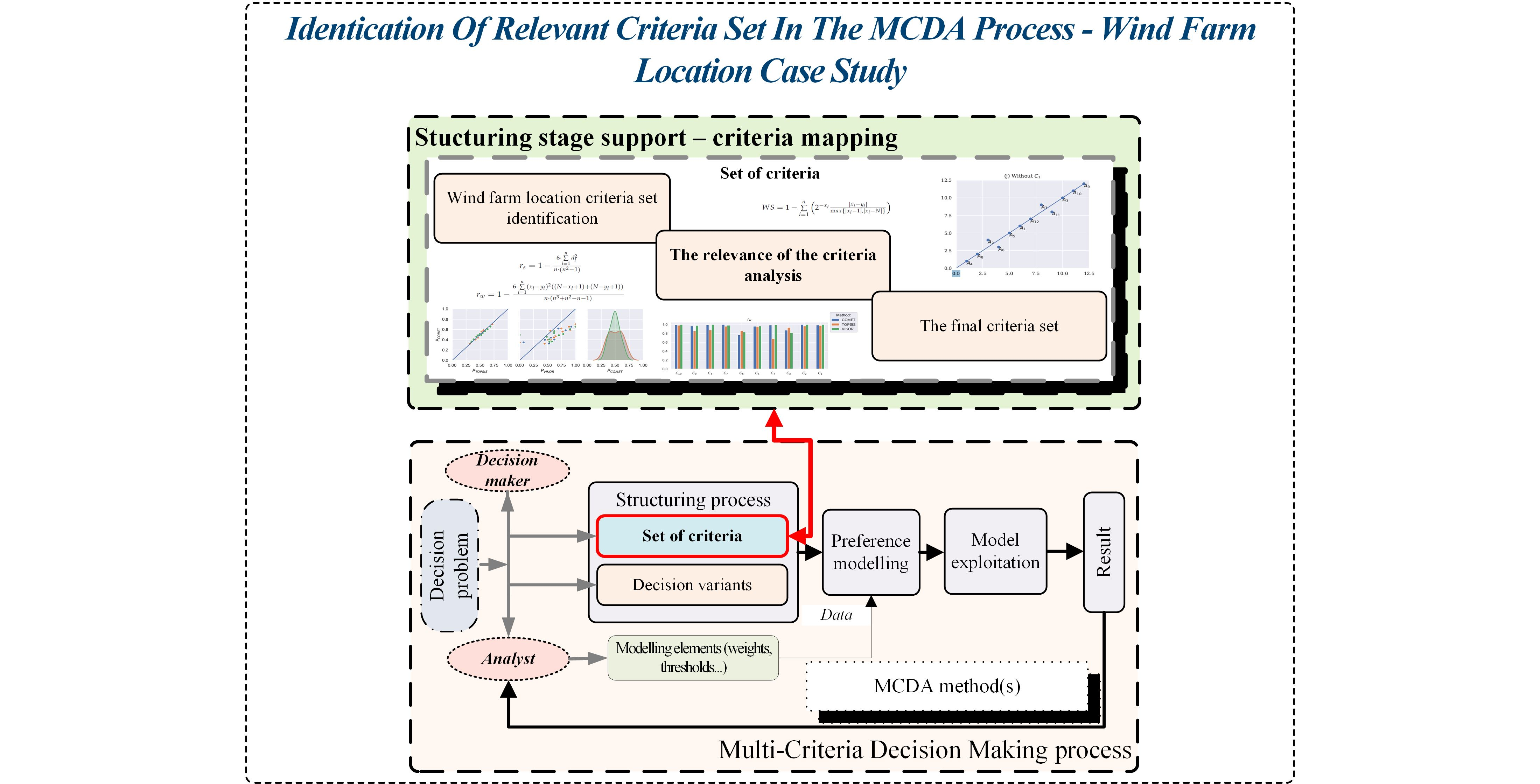
The problem studied in this paper concerns the objectification of a set of criteria in a given decision problem. For this purpose, the authors developed a framework (see Figure 2) composed of two basic methodological elements: (1) a set of reference MCDA methods (TOPSIS, VIKOR, COMET); and (2) a set of similarity coefficients (Spearman correlation coefficients and WS coefficient). These elements are the basis for further relevance analysis of individual criteria in a considered MCDA model. In the first step, a primary ranking (including all the criteria for the given model) was computed, which in further studies was treated as the reference ranking. Subsequently, using the indicated MCDA methods, a set of rankings was prepared in which iteratively a single criterion was excluded. This was the basis for testing the similarity of the obtained solutions to the reference solution, as well as for the recommendations in terms of both indicating the high significance and possible elimination of individual criteria of the original model. In the subsequent research steps, the number of criteria eliminated from the original model was extended to 2 and 3, once again examining the similarities of the obtained sets of rankings with the reference solution. When carrying out the analysis for reference points, both the final rankings and utility function values of individual decision variants were taken into account. As a result of a detailed analysis of the obtained results, recommendations were obtained regarding the reference criteria set for the decision problem under consideration.

It is worth noting that there is a significant similarity between these three methods—TOPSIS and VIKOR methods are based on the same assumptions—reference points. They differ only in the adopted techniques of normalization and data aggregation [96]. The TOPSIS method assumes minimizing the distance to the ideal solution and maximizing the distance from the anti-ideal solution [51]. In contrast, the VIKOR method minimizes only the distance to the ideal solution [97], which in practice results in the desired significant reduction of substitution of individual criteria. In the TOPSIS method, the normalization is vectorized, while in the VIKOR method, it is linear [96]. The COMET method is based on the space of so-called characteristic objects. This technique solves the problem of the ranking reversal paradox, because it compares characteristic objects instead of the alternatives. The principles of the COMET, TOPSIS and VIKOR methods, as mentioned above, make them a comprehensive group of methods based on the so-called “reference points”. It is worth noting that TOPSIS does not require identification of the dependence of component attributes (criteria) of the decision model [50,98,99]. The situation is similar for the COMET method. However, additionally, the method secretly identifies the weights of attributes and allows to model any form of preference function [100,101]. The above indications show a great potential of using the whole group of methods indicated. What is important is that it can be successfully applied even in cases in which we do not yet have full scientific knowledge about dependencies or independence of model attributes [96,102].

3.2. The TOPSIS Method

The concept of the TOPSIS method is to specify the distance of the considered objects from the ideal and anti-ideal solution [99,103,104]. The final effect of the study is a synthetic coefficient which forms a ranking of the studied objects. The best object is defined as the one with the shortest distance from the ideal solution and, at the same time, the most considerable distance from the anti-ideal solution [105,106]. The formal description of the TOPSIS method should be shortly mentioned [50]:

Step 1. Create a decision matrix consisting of n alternatives with the values of criteria k. Then normalize the decision matrix according to the Equation (1).

$$r_{ij}=\frac{x_{ij}}{\sqrt{(\sum x_{ij}^2)}}$$

(1)

where $x_{ij}$ and $r_{ij}$ are the initial and normalized value of the decision matrix.

Step 2. Then create a weighted decision matrix that has previously been normalized according to the Equation (2).

$$v_{ij}=w_j{r}_{ij}$$

(2)

where $v_{ij}$ is the value of the weighted normalized decision matrix and $w_j$ is the weight for j criterion.

Step 3. Determine the best and worst alternative according to the following Equation (3):

$$\begin{array}{c}{A}_{*}=\{v_1^{*},\cdots ,v_n^{*}\}\\ A_{\prime }=\{v_1^{\prime },\cdots ,v_n^{\prime }\}\end{array}$$

(3)

where:

$$\begin{array}{c}{v}_j^{*}=\{max\left(v_{ij}\right)\mathrm{if}j\in J;min\left(v_{ij}\right)\mathrm{if}j\in J^{\prime }\}\\ v_j^{\prime }=\{min\left(v_{ij}\right)\mathrm{if}j\in J;max\left(v_{ij}\right)\mathrm{if}j\in J^{\prime }\}\end{array}$$

Step 4. Calculate the separation measure from the best and worst alternative for each decision variant according to the Equation (4).

$$\begin{array}{c}{S}_i^{*}=\sqrt{\sum {(v_j^{*}-v_{ij})}^2}\\ S_i^{\prime }=\sqrt{\sum {(v_j^{*}-v_{ij})}^2}\end{array}$$

(4)

Step 5. Calculate the similarity to the worst condition by equation:

$$C_i^{*}=\frac{S_i^{\prime }}{(S_i^{*}+S_i^{\prime })}$$

(5)

Step 6. Rank the alternatives by their similarity to the worst state.

3.3. The VIKOR Method

The VIKOR method was developed to solve a discrete decision problem with conflicting criteria. The technique focuses on ranking and choosing from a set of alternatives, and finding compromise solutions for the problem [107]. It can be presented in the following steps [108,109]:

Step 1. Create a decision matrix consisting of n alternatives with the values of criteria k. Then normalize the decision matrix according to the Equation (6).

$$r_{ij}=\frac{x_{ij}}{\sqrt{(\sum x_{ij}^2)}}$$

(6)

where $x_{ij}$ and $r_{ij}$ are the initial and normalized value of the decision matrix.

Step 2. Define ideal $A^{*}$ and negative-ideal $A^{-}$ alternatives following the Equation (7):

$$\begin{array}{c}\begin{array}{cc}\hfill A^{*}& =\left\{\left(max{f}_{ij}\mid j\in J\right) or \left(min{f}_{ij}\mid j\in J^{\prime }\right)\mid i=1,2,\cdots ,m\right\}\hfill \\ \hfill & =\left\{f_1^{*},f_2^{*},\dots ,f_j^{*},\dots f_n^{*}\right\}\hfill \end{array}\\ \begin{array}{cc}\hfill A^{-}& =\left\{\left(min{f}_{ij}\mid j\in J\right) or \left(max{f}_{ij}\mid j\in J^{\prime }\right)\mid i=1,2,\cdots ,m\right\}\hfill \\ \hfill & =\left\{f_1^{-},f_2^{-},\cdots ,f_j^{-},\cdots ,f_n^{-}\right\}\hfill \end{array}\end{array}$$

(7)

where

$$\begin{array}{c}J=\left\{j=1,2,\dots ,n\mid f_{ij},\right.\mathrm{a}\mathrm{larger}\mathrm{response}\mathrm{is}\mathrm{desired}\}\\ J^{\prime }=\left\{j=1,2,\dots ,n\mid f_{ij},\right.\mathrm{a}\mathrm{smaller}\mathrm{response}\mathrm{is}\mathrm{desired}\}\end{array}$$

Step 3. Determine the utility $S_i$ and regret $R_i$ measure using the Equations (8) and (9).

$$S_i=\sum _{j=1}^n{w}_j\left(f_j^{*}-f_{ij}\right)/\left(f_j^{*}-f_j^{-}\right)$$

(8)

$$R_i=\underset{j}{max}\left[w_j\left(f_j^{*}-f_{ij}\right)/\left(f_j^{*}-f_j^{-}\right)\right]$$

(9)

where $w_j$ is the weight of the jth criterion.

Step 4. By using the Equation (10) the VIKOR index should be evaluated.

$$Q_i=\nu \left[\frac{S_i-S^{*}}{S^{-}-S^{*}}\right]+(1-\nu )\left[\frac{R_i-R^{*}}{R^{-}-R^{*}}\right]$$

(10)

where

$$\begin{array}{c}{S}^{*}={\displaystyle \underset{i}{min}}{S}_i,S^{-}={\displaystyle \underset{i}{max}}{S}_i\\ R^{*}={\displaystyle \underset{i}{min}}{R}_i,R^{-}={\displaystyle \underset{i}{max}}{R}_i\end{array}$$

where v is determined as the strategy weighting. In this case, it is equal 0.5.

Step 5. Rank the alternatives, sorting by the values Q, from the minimum value. In this way we obtained the final rank rank.

3.4. The COMET Method

Many MCDM methods exhibit the rank reversal phenomenon, however, the Characteristic Objects Method (COMET) is completely free of this problem [110]. In previous works, the accuracy of the COMET method was verified [102,111]. The formal notation of the COMET method should be briefly recalled [42,101,112]:

Step 1. Definition of the space of the problem - the expert determines the dimensionality of the problem by selecting r criteria, $C_1,C_2,\dots ,C_r$. Then, a set of fuzzy numbers is selected for each criterion $C_i$, e.g., $\{{\tilde{C}}_{i1},{\tilde{C}}_{i2},\dots ,{\tilde{C}}_{i{c}_i}\}$ (11):

$$\begin{array}{c}{C}_1=\left\{{\tilde{C}}_{11},{\tilde{C}}_{12},\dots ,{\tilde{C}}_{1c_1}\right\}\\ C_2=\left\{{\tilde{C}}_{21},{\tilde{C}}_{22},\dots ,{\tilde{C}}_{2c_1}\right\}\\ \cdots \\ C_r=\left\{{\tilde{C}}_{r1},{\tilde{C}}_{r2},\dots ,{\tilde{C}}_{r{c}_r}\right\}\end{array}$$

(11)

where $C_1,C_2,\dots ,C_r$ are the ordinals of the fuzzy numbers for all criteria.

Step 2. Generation of the characteristic objects—the characteristic objects ($CO$) are obtained with the usage of the Cartesian product of the fuzzy numbers’ cores of all the criteria (12):

$$CO=\langle C\left(C_1\right) \times C\left(C_2\right) \times \cdots \times C\left(C_r\right)\rangle$$

(12)

As a result, an ordered set of all $CO$ is obtained (13):

$$\begin{array}{c}C{O}_1=\langle C\left({\tilde{C}}_{11}\right),C\left({\tilde{C}}_{21}\right),\dots ,C\left({\tilde{C}}_{r1}\right)\rangle \\ C{O}_2=\langle C\left({\tilde{C}}_{11}\right),C\left({\tilde{C}}_{21}\right),\dots ,C\left({\tilde{C}}_{r1}\right)\rangle \\ \cdots \\ C{O}_t=\langle C\left({\tilde{C}}_{1c_1}\right),C\left({\tilde{C}}_{2c_2}\right),\dots ,C\left({\tilde{C}}_{r{c}_r}\right)\rangle \end{array}$$

(13)

where t is the count of $CO$s and is equal to (14):

$$t=\prod _{i=1}^r{c}_i$$

(14)

Step 3. Evaluation of the characteristic objects—the expert determines the Matrix of Expert Judgment ($MEJ$) by comparing the $CO$s pairwise. The matrix is presented below (15):

$$MEJ=\left(\begin{array}{cccc}{\alpha }_{11}& {\alpha }_{12}& \cdots & {\alpha }_{1t}\\ {\alpha }_{21}& {\alpha }_{22}& \cdots & {\alpha }_{2t}\\ \cdots & \cdots & \cdots & \cdots \\ {\alpha }_{t1}& {\alpha }_{t2}& \cdots & {\alpha }_{tt}\end{array}\right)$$

(15)

where ${\alpha }_{ij}$ is the result of comparing $C{O}_i$ and $C{O}_j$ by the expert. The function $C_{exp}$ denotes the mental judgement function of the expert. It depends solely on the knowledge of the expert. The expert’s preferences can be presented as (16):

$${\alpha }_{ij}=\left\{\begin{array}{c}0.0,f_{exp}\left(C{O}_i\right) <f_{exp}\left(C{O}_j\right)\hfill \\ 0.5,f_{exp}\left(C{O}_i\right) =f_{exp}\left(C{O}_j\right)\hfill \\ 1.0,f_{exp}\left(C{O}_i\right) >f_{exp}\left(C{O}_j\right)\hfill \end{array}\right.$$

(16)

After the MEJ matrix is prepared, a vertical vector of the Summed Judgments ($SJ$) is obtained as follows (17):

$$S{J}_i=\sum _{j=1}^t{\alpha }_{ij}$$

(17)

Eventually, the values of preference are approximated for each characteristic object. As a result, a vertical vector P is obtained, where the i-th row contains the approximate value of preference for $C{O}_i$.

Step 4. The rule base—each characteristic object and its value of preference is converted to a fuzzy rule as (18):

$$IFC\left({\tilde{C}}_{1i}\right)ANDC\left({\tilde{C}}_{2i}\right)AND\dots THEN{P}_i$$

(18)

In this way, a complete fuzzy rule base is obtained.

Step 5. Inference and the final ranking—each alternative is presented as a set of crisp numbers, e.g., $A_i=\{a_{i1},a_{i2},a_{ri}\}$. This set corresponds to the criteria $C_1,C_2,\dots ,C_r$. Mamdani’s fuzzy inference method is used to compute the preference of the i-th alternative. The rule base guarantees that the obtained results are unequivocal. The whole process of the COMET method is presented on the Figure 3.

3.5. Similarity Coefficients

The similarity coefficients of the rankings allow to compare how different is the order of variants in both compared rankings. It is important to choose such coefficients that work well in the decision-making field. The paper uses three such coefficients, i.e., Spearman correlation coefficient (19), Spearman weighted correlation coefficient (20) and WS similarity coefficients (21) [114]. The simplest way is to check whether the rankings are equal. The much more common way is to use one of the coefficients of the dependence for two variables, where the obtained rankings for a set of alternatives are our variables. The most frequently used symmetrical coefficient is the Spearman’s coefficient.

$$\begin{array}{c}{r}_s=1-\frac{6·{\displaystyle \sum _{i=1}^n}{d}_i^2}{n·\left(n^2-1\right)}\hfill \end{array}$$

(19)

where $d_i$ is defined as the difference between the ranks $d_i=x_i-y_i$ and n is the number of elements in the ranking.

The weighted rank measure of correlation $r_w$ is also symmetric coefficient which was shown in [115]. The equation is presented as (20):

$$\begin{array}{c}{r}_w=1-\frac{6·{\displaystyle \sum _{i=1}^n}{(x_i-y_i)}^2((N-x_i+1)+(N-y_i+1))}{n·\left(n^3+n^2-n-1\right)}\hfill \end{array}$$

(20)

WS coefficient is a new ranking similarity factor, which is sensitive to significant changes in the ranking. This new indicator is strongly related to the difference between two rankings on particular positions. The ranking top has a more significant influence on similarity than the bottom of the ranking [114]. WS coefficient is asymmetrical, and the equation is presented as (21):

$$\begin{array}{c}WS=1-{\displaystyle \sum _{i=1}^n}\left(2^{-x_i}\frac{|x_i-y_i|}{\max \left\{\right|x_i-1|,|x_i-N\left|\right\}}\right)\hfill \end{array}$$

(21)

4. Results and Discussion

The practical organization of the research experiments presented below is as follows. The following Section 4.1 presents the similarity analysis of the rankings obtained by the TOPSIS method, assuming the elimination of any single criterion from the reference model. Similarly, the results obtained with the VIKOR and COMET methods can be found in Appendix A and Appendix B. Section 4.2 includes similarity rank studies as above, assuming the elimination of pairs of criteria from the original model. Here, too, the TOPSIS method was used. Additionally, the results of using the VIKOR and COMET methods are included in Appendix C and Appendix D. Similarly, the research was extended for the purposes of possible elimination of 3 criteria from the reference model. The results of the TOPSIS method are presented in Section 4.3, while the results of the VIKOR and COMET methods are available in Appendix E and Appendix F. A synthetic analysis of the tests performed for all 3 MCDA methods is presented in Section 4.4. Due to the fact that the analyzes so far used only the positions of decision variants in the rankings, in the next Section 4.5 a full quantitative analysis of the similarity of rankings was carried out, using its value of the utility function instead of the rank of a given decision variant. This made it possible to more precisely indicate the areas of relevance of the analyzed criteria of the decision model.

The three MCDA methods presented in Section 3 i.e., COMET, TOPSIS and VIKOR have been utilized to determine the similarity of alternative datasets rankings. For this purpose, an exemplary wind farm location problem [95] was chosen, from which a set of criteria and a set of alternatives were taken (see

Table 1. Selected criteria $C_1$–$C_{10}$ with names and their units and type [95].

${\mathit{C}}_{\mathit{i}}$	Criterion	Unit	Preference Direction
$C_1$	yearly amount of energy generated	(MWh)	Max
$C_2$	average wind speed at the height of 100 m	(m/s)	Max
$C_3$	distance from power grid connection	(km)	Min
$C_4$	power grid voltage on the site of connection and its vicinity	(kV)	Max
$C_5$	distance from the road network	(km)	Min
$C_6$	location in Natura 2000 protected area	[0;1]	Min
$C_7$	social acceptance	(%)	Max
$C_8$	investment cost	(PLN)	Min
$C_9$	operational costs per year	(PLN)	Min
$C_{10}$	profits from generated energy per year	(PLN)	Max

). The types of criteria are divided equally, with half of them being of cost type and half of them being the benefit type. The

Table 2. Set of alternatives $A_1$–$A_{12}$ with their criteria values.

${\mathit{A}}_{\mathit{i}}$	${\mathit{C}}_1$	${\mathit{C}}_2$	${\mathit{C}}_3$	${\mathit{C}}_4$	${\mathit{C}}_5$	${\mathit{C}}_6$	${\mathit{C}}_7$	${\mathit{C}}_8$	${\mathit{C}}_9$	${\mathit{C}}_{10}$
$A_1$	106.78	6.75	2.00	220	6.00	1	52.00	455.50	8.90	36.80
$A_2$	86.37	7.12	3.00	400	10.00	0	20.00	336.50	7.20	29.80
$A_3$	104.85	6.95	60.00	220	7.00	1	60.00	416.00	8.70	36.20
$A_4$	46.60	6.04	1.00	220	3.00	0	50.00	277.00	3.90	16.00
$A_5$	69.18	7.05	33.16	220	8.00	0	35.49	364.79	5.39	33.71
$A_6$	66.48	6.06	26.32	220	6.53	0	34.82	304.02	4.67	27.07
$A_7$	74.48	6.61	48.25	400	4.76	1	44.19	349.45	4.93	28.89
$A_8$	73.67	6.06	19.54	400	3.19	0	46.41	354.65	8.01	21.09
$A_9$	100.58	6.37	39.27	220	8.43	1	22.07	449.42	7.89	17.62
$A_{10}$	94.81	6.13	50.58	220	4.18	1	21.14	450.88	5.12	17.30
$A_{11}$	48.93	7.12	21.48	220	5.47	1	55.72	454.71	8.39	19.16
$A_{12}$	74.75	6.58	7.08	400	9.90	1	26.01	455.17	4.78	18.44

presents a set of alternatives and contains 12 decision-making variants. The similarity of the reference ranking of a particular method with the ranking in which a particular criterion was excluded by means of similarity indicators was examined. The reference ranking was obtained by assessing the alternatives based on all defined criteria.

4.1. Rankings Comparison—One Criterion Excluded Case

The rankings of alternatives of particular variants of exclusion criteria and similarity coefficients of these rankings with the reference ranking for TOPSIS method are placed in

Table 3. Rankings of alternatives with similarity coefficients and distance for criteria not included in the ranking process (method: TOPSIS).

Excl.	${\mathit{A}}_1$	${\mathit{A}}_2$	${\mathit{A}}_3$	${\mathit{A}}_4$	${\mathit{A}}_5$	${\mathit{A}}_6$	${\mathit{A}}_7$	${\mathit{A}}_8$	${\mathit{A}}_9$	${\mathit{A}}_{10}$	${\mathit{A}}_{11}$	${\mathit{A}}_{12}$	WS	${\mathit{r}}_{\mathit{w}}$	${\mathit{r}}_{\mathit{s}}$	Distance
None	5	3	10	1	6	4	9	2	12	11	8	7	1.0000	1.0000	1.0000	0.0000
$C_{10}$	5	3	11	1	6	4	9	2	12	10	8	7	0.9998	0.9973	0.9930	0.0771
$C_9$	4	3	10	2	6	5	9	1	12	11	8	7	0.9172	0.9784	0.9860	0.0600
$C_8$	5	3	10	1	6	4	9	2	12	11	8	7	1.0000	1.0000	1.0000	0.0145
$C_7$	5	2	11	1	6	4	8	3	12	10	9	7	0.9601	0.9811	0.9790	0.1020
$C_6$	1	4	10	2	9	6	8	3	12	11	7	5	0.8709	0.8327	0.8671	0.2042
$C_5$	5	1	10	2	6	4	9	3	11	12	8	7	0.9016	0.9628	0.9720	0.1180
$C_4$	5	4	10	1	6	3	9	2	12	11	8	7	0.9782	0.9897	0.9930	0.0559
$C_3$	8	5	7	2	4	3	6	1	12	9	10	11	0.8678	0.8165	0.7832	0.2738
$C_2$	5	3	10	1	6	4	9	2	12	11	8	7	1.0000	1.0000	1.0000	0.0037
$C_1$	5	3	10	1	6	4	9	2	12	11	8	7	1.0000	1.0000	1.0000	0.0890

. The reference ranking in the table is presented as the excluded “None” criterion. The rankings created with the excluded criteria $C_1$, $C_2$ and $C_8$ have the biggest correlation with the reference ranking among the considered variants. However, it should be mentioned that the ranking distance created with the exclusion of criterion $C_1$ is much bigger than in case of exclusion of criterion $C_4$, $C_9$ and $C_{10}$ from the ranking process, where $C_1$ has much bigger values of similarity indicators [116]. For the criteria excluded from the ranking process $C_{10}$, $C_7$ and $C_4$, the correlation between the resulting ranking and the reference ranking is high. For the excluded criteria $C_9$ and $C_5$, the correlation between the created rankings and the reference ranking reflected by the similarity indicators is large. However, there is also a great difference between the indicators. The $WS$ ratio is much smaller than the $r_s$ and $r_w$ ratios in both cases. The smallest correlation can be seen in the rankings that are created when the $C_3$ and $C_6$ criteria are excluded. These rankings have the greatest distance from the reference ranking.

The charts showing relations between the reference ranking and the ranking, excluding one criterion for the TOPSIS method, are presented using the Figure 4. The x-axis shows the values of the reference ranking. The y-axis presents the values of the ranking in which a given criterion was excluded. The highest similarity among the considered rankings with excluded criteria and the reference ranking is noticeable for the criteria $C_1$, $C_2$ and $C_8$. The alternatives in these rankings do not differ from the reference ranking. Slightly less similarity between the rankings is visible in charts (a) and (g) for the criterion excluded from the ranking process $C_{10}$ and $C_4$. Rankings differ in their alternatives on two positions. For the criteria, $C_9$ and $C_7$ excluded from the ranking process, the similarity to the reference ranking differs on four positions and six positions respectively. In the case where the $C_5$ criterion from the evaluation of alternatives is $C_5$, the obtained ranking compared to the reference ranking differs on five positions. The lowest similarity among the considered rankings with excluded criteria and the reference ranking is noticeable for criterion $C_5$ and $C_3$, where the positions in the rankings were the same for the alternative $A_8$ for criterion $C_3$ and for the alternatives $A_2$, $A_9$ and $A_8$ for the excluded criterion $C_5$.

4.2. Rankings Comparison—Two Criteria Excluded Case

The rankings of alternatives of particular variants of exclusion pairs of criteria and similarity coefficients of these rankings with the reference ranking for TOPSIS method are presented in

Table 4. Rankings of alternatives with similarity and distance coefficients for criterion pairs not included in the ranking process (method: TOPSIS).

Excl.	${\mathit{A}}_1$	${\mathit{A}}_2$	${\mathit{A}}_3$	${\mathit{A}}_4$	${\mathit{A}}_5$	${\mathit{A}}_6$	${\mathit{A}}_7$	${\mathit{A}}_8$	${\mathit{A}}_9$	${\mathit{A}}_{10}$	${\mathit{A}}_{11}$	${\mathit{A}}_{12}$	WS	${\mathit{r}}_{\mathit{w}}$	${\mathit{r}}_{\mathit{s}}$	Distance
None	5	3	10	1	6	4	9	2	12	11	8	7	1.0000	1.0000	1.0000	0.0000
$C_{10}{C}_2$	5	3	11	1	6	4	9	2	12	10	8	7	0.9998	0.9973	0.9930	0.0808
$C_9{C}_2$	4	3	10	2	6	5	9	1	12	11	8	7	0.9173	0.9785	0.9860	0.0606
$C_8{C}_2$	5	3	10	1	6	4	9	2	12	11	8	7	1.0000	1.0000	1.0000	0.0138
$C_7{C}_2$	5	2	11	1	6	4	8	3	12	10	9	7	0.9602	0.9812	0.9790	0.1037
$C_6{C}_2$	1	4	10	2	9	6	8	3	12	11	7	5	0.8710	0.8327	0.8671	0.2033
$C_5{C}_2$	5	1	10	2	6	4	9	3	11	12	8	7	0.9017	0.9629	0.9720	0.1173
$C_4{C}_2$	5	4	10	1	6	3	9	2	12	11	8	7	0.9783	0.9898	0.9930	0.0573
$C_3{C}_2$	8	5	7	2	4	3	6	1	12	9	10	11	0.8679	0.8166	0.7832	0.2747
$C_1{C}_2$	5	3	10	1	6	4	9	2	12	11	8	7	1.0000	1.0000	1.0000	0.0912

. The reference ranking in the table is presented as the excluded “None” criterion. For the rankings created from excluded criterion pairs $C_1{C}_2$ and $C_8{C}_2$, the similarity with the reference ranking is the highest. The resulting rankings have a value of 1 for all the similarity coefficients under consideration. However, in case of the ranking created with the exclusion of criteria pair $C_1{C}_2$ the preference distance of this ranking with reference ranking preference is greater than in case of rankings created with the exclusion of criterion pair $C_{10}{C}_2$, $C_9{C}_2$ and $C_4{C}_2$. Rankings created with excluded criteria pairs $C_4{C}_2$, $C_7{C}_2$ and $C_{10}{C}_2$ had slightly less correlation with the reference ranking. For rankings with excluded criteria pairs $C_9{C}_2$ and $C_5{C}_2$ the difference between the values of similarity ratios $r_w$ and $r_s$ and $WS$ is large. It means that according to the $WS$ similarity coefficient, the correlation between the rankings mentioned above and the reference ranking is small.

On the other hand, according to the $r_w$ and $r_s$ similarity coefficient, the correlation is large. The smallest similarity between the reference ranking exists for the rankings from which the $C_3{C}_2$ and $C_6{C}_2$ criteria pairs are excluded. There is a big difference between the similarity coefficients $WS$ and $r_w$ and the $r_s$ coefficient for a ranking that excludes the $C_3{C}_2$ criterion pair. In the case of a ranking that excludes the $C_6{C}_2$ pair of criteria, all the similarity coefficients under consideration differ significantly.

The graphs showing the dependencies of the rankings in which pairs of criteria were excluded from the reference chart for the TOPSIS method have been visualized using the Figure 5. Rankings that have the same alternative positions as the reference chart was created with the criteria pair $C_8{C}_2$ and $C_1{C}_2$ excluded. The slightly worse similarity to the reference ranking are rankings which exclude criteria pairs $C_3{C}_2$ and $C_{10}{C}_2$. These rankings differ from the reference ranking only on two positions. This means that these criteria do not have too much influence in the ranking process. The least similar rankings to the reference ranking were created with the exclusion of criterion pairs $C_3{C}_2$ and $C_6{C}_2$. Most of the alternatives have entirely different positions than in the reference ranking, so the pairs of these criteria are significant in the ranking process. Rankings that have been created by excluding the rest of the criteria pairs differ from the reference ranking of four, five or six positions.

4.3. Rankings Comparison—Three Criteria Excluded Case

Rankings of alternatives of particular variants of the triple criteria exclusions and similarity coefficients of these rankings with the reference ranking for TOPSIS method are placed in

Table 5. Rankings of alternatives with similarity and distance factors for triad of criteria not included in the ranking process (method: TOPSIS).

Excl.	${\mathit{A}}_1$	${\mathit{A}}_2$	${\mathit{A}}_3$	${\mathit{A}}_4$	${\mathit{A}}_5$	${\mathit{A}}_6$	${\mathit{A}}_7$	${\mathit{A}}_8$	${\mathit{A}}_9$	${\mathit{A}}_{10}$	${\mathit{A}}_{11}$	${\mathit{A}}_{12}$	WS	${\mathit{r}}_{\mathit{w}}$	${\mathit{r}}_{\mathit{s}}$	Distance
None	5	3	10	1	6	4	9	2	12	11	8	7	1.0000	1.0000	1.0000	0.0000
$C_{10}{C}_2{C}_7$	5	3	12	1	6	4	9	2	11	10	8	7	0.9997	0.9935	0.9790	0.1693
$C_9{C}_2{C}_7$	5	2	11	3	6	4	9	1	12	10	8	7	0.8700	0.9618	0.9720	0.1151
$C_8{C}_2{C}_7$	5	2	11	1	6	4	9	3	12	10	8	7	0.9610	0.9860	0.9860	0.1032
$C_6{C}_2{C}_7$	1	3	11	2	9	6	7	4	12	10	8	5	0.8600	0.8139	0.8462	0.2011
$C_5{C}_2{C}_7$	6	1	11	2	5	4	9	3	10	12	8	7	0.8945	0.9500	0.9510	0.2428
$C_4{C}_2{C}_7$	6	2	11	1	5	4	9	3	12	10	8	7	0.9539	0.9779	0.9790	0.1193
$C_3{C}_2{C}_7$	7	5	9	3	4	2	6	1	11	8	12	10	0.8194	0.8031	0.7692	0.3153
$C_1{C}_2{C}_7$	6	3	11	1	5	4	9	2	12	10	8	7	0.9928	0.9892	0.9860	0.1571

. The reference ranking in the table is presented as the excluded “None” criterion. The highest similarity to the reference ranking was achieved by excluding the three criteria $C_{10}{C}_2{C}_7$. It has the highest values of similarity indicators $WS$ and $r_w$ from the considered rankings with the exclusion of the three criteria. However, its distance to the reference ranking is much greater than in the case of rankings from which the three criteria were excluded $C_9{C}_2{C}_7$, $C_8{C}_2{C}_7$, $C_4{C}_2{C}_7$ and $C_1{C}_2{C}_7$. It should also be mentioned that the $r_s$ similarity ratio for a ranking with the three criteria, $C_{10}{C}_2{C}_7$ does not have the highest value from the table. The resemblance to the reference ranking with the rankings that were created when the three criteria $C_8{C}_2{C}_7$, $C_4{C}_2{C}_7$ and $C_1{C}_2{C}_7$ are similar to the resemblance to the reference ranking with the ranking in which the three criteria $C_{10}{C}_2{C}_7$ were excluded. However, the $WS$ coefficient value for this ranking is much higher than the $WS$ coefficient values of other rankings. The big difference between the $WS$ similarity coefficient and the similarity coefficients $r_w$ and $r_s$ have rankings that were created when the three criteria $C_5{C}_2{C}_7$ and $C_9{C}_2{C}_7$ were excluded. The value of the $WS$ coefficient in these rankings is much smaller than in the case of the $r_w$ and $r_s$ coefficients. This means that according to these ratios, there is a strong correlation between these rankings with excluded criteria and the reference ranking. In case of the rankings from which the three criteria $C_6{C}_2{C}_7$ and $C_3{C}_2{C}_7$ have been excluded, the similarity indicators considered received the lowest values. This means that the data of the three criteria have a significant influence on the final ranking. Distances for the rankings from which data of three criteria were excluded were also given the highest values from the considered rankings.

In the charts illustrating the relationship between the rankings in which three criteria were excluded, and the reference chart for the TOPSIS method were visualized using the Figure 6. The values of reference ranking are on x-axis, and y-axis, there are values of the ranking that was created when the three criteria were excluded. The most similar to the reference ranking is the ranking that excludes the three criteria $C_{10}{C}_2{C}_7$. The three criteria are of low importance for the ranking process. The three criteria are less similar to the reference ranking and do not include the three criteria $C_1{C}_2{C}_7$, $C_8{C}_2{C}_7$ and $C_9{C}_2{C}_7$. Rankings with the excluded triple criteria $C_1{C}_2{C}_7$ and $C_8{C}_2{C}_7$ differ from the reference ranking of four positions while ranking with excluded triple criteria $C_9{C}_2{C}_7$ differs from the reference ranking of five positions. The ranking that excludes the three criteria, $C_4{C}_2{C}_7$ and $C_5{C}_2{C}_7$ has little similarity to the reference ranking. For the ranking from which the three criteria $C_4{C}_2{C}_7$ have been excluded differ in six positions, while the ranking from which the criteria $C_5{C}_2{C}_7$ have been excluded differ in eight positions with a reference ranking. The least similarity to the reference ranking has a ranking that excludes the three criteria $C_3{C}_2{C}_7$ and $C_6{C}_2{C}_7$. In case of a ranking from which three criteria $C_6{C}_2{C}_7$ have been excluded, it has three positions as the reference ranking. In contrast, the ranking from which criteria $C_3{C}_2{C}_7$ have been excluded does not have the same positions as the reference ranking. It means that the aforementioned three criteria have the most significant influence on the ranking process.

4.4. Results Analysis and Discussion

In order to graphically present the relations of the MCDA methods used and their impact on $WS$ and $r_s$ coefficients values, histograms were used (see Figure 7, Figure 8 and Figure 9). The Figure 7 chart refers to rankings in which one given criterion has been excluded. It shows a large difference between the $WS$ coefficient and the $r_w$ coefficient. The $r_w$ ratio has a much higher value than the $WS$ ratio for the $C_9$ criterion for COMET and VIKOR methods. On the other hand, in case of the $C_6$ criterion excluded, the $WS$ ratio has a greater value than the $r_w$ ratio for COMET method. The value of the $r_w$ similarity coefficient is greater than the $WS$ similarity coefficient for the $C_5$ criterion for the COMET method and the VIKOR method. Both coefficients for the TOPSIS method have relatively similar values. The rest of the considered coefficient values are also similar for COMET and VIKOR methods.

Similarity coefficients relating to the pairs of criteria are presented in the chart Figure 8. In case of the $C_9{C}_2$ criteria pair the COMET method, and the VIKOR method has a greater value of $r_w$ than $WS$. Meanwhile, for criterion pair $C_7{C}_2$ a smaller value than $r_w$ has a $WS$ similarity factor for VIKOR method. Whereas for the criteria pair $C_3{C}_2$ a smaller value has the $r_w$ ratio for the VIKOR method. When using COMET for the $C_6{C}_2$ criteria pair, the $r_w$ ratio has a smaller value than the $WS$ ratio. For TOPSIS method the $WS$ similarity factor for criteria pairs $C_5{C}_2$, $C_4{C}_2$ and $C_1{C}_2$ has a greater value than the $r_w$ similarity factor.

The similarity coefficients for the three criteria have been visualized using the graph on Figure 9. In the case of the triple criteria, $C_9{C}_2{C}_7$ and $C_5{C}_2{C}_7$, the $r_w$ similarity coefficient has a greater value than the $WS$ coefficient for VIKOR and COMET methods. With three criteria $C_8{C}_2{C}_7$ and $C_1{C}_2{C}_7$ the $WS$ coefficient has a smaller value than the $r_w$ coefficient for TOPSIS methods. In the COMET method, the three criteria $C_6{C}_2{C}_7$ have a greater value of $WS$ than $r_w$. However, for the three criteria $C_3{C}_2{C}_7$ the $WS$ value is much smaller than the $r_w$ value for the COMET method. The value of $r_w$ for the three criteria $C_4{C}_2{C}_7$ is smaller than the value of $WS$ for TOPSIS method. However, for the $C_3{C}_2{C}_7$ three criteria, the $WS$ similarity factor has a smaller value than the $r_w$ similarity factor for the TOPSIS method.

4.5. Results Analysis Based on Utility Values of Decision Variants

Contrary to the previous sections, in this section, a quantitative analysis of the result rankings was carried out based on the resultant utility value of the alternatives in particular rankings. This analysis is important, as it provides a more complete and valuable insight of the effects of excluding particular criteria of the decision-making model. It is worth recalling that in the previous sections, only the place of alternatives in the rankings was examined. Here, the study was also conducted by excluding 1, 2 and 3 criteria in turn. Figure 10, Figure 11 and Figure 12 present obtained results.

On Figure 10, the calculated utility values for alternatives to COMET, VIKOR and TOPSIS for single exclusion criteria are presented. The “None” criterion means that no criterion is excluded. The differences between the utility values of alternatives to COMET and TOPSIS methods are minimal. On the other hand, the differences are large between the utility values of alternatives from VIKOR and COMET, and between the utility values of alternatives from VIKOR and TOPSIS. The utility values of alternatives to the VIKOR method are much more valuable than utility values of alternatives to COMET and TOPSIS. The utility values of alternatives from COMET method with excluded criterion $C_2$ and non-excluded criterion are almost identical.

On the other hand, the utility values of the alternatives with the excluded criterion $C_6$ are much higher than those of the non-excluded criterion and the excluded criterion $C_2$. In the case of the VIKOR method, the differences between the utility values for the excluded criteria are not as significant as for COMET method. The utility values of alternatives with the excluded criterion $C_6$ have more similar values to the reference utility values of alternatives than the utility values of alternatives with excluded criterion $C_2$. In the TOPSIS method, the alternatives’ utility values for the excluded criterion $C_2$ and the non-excluded criterion are very similar to each other. On the other hand, in the case of utility values for the excluded criterion $C_6$, the difference in value with the utility values of alternatives for the excluded criterion $C_2$ and the non-excluded criterion is massive. The utility values of alternatives for the excluded criterion $C_6$ have the highest value of the considered preferences.

The calculated utility values of alternatives using TOPSIS, VIKOR and COMET methods for exclusion pairs of criteria have been visualized in the picture Figure 11. The “None” criterion means that no criterion is excluded. The utility values of the TOPSIS and COMET alternatives are similar. However, in case of the utility values for the VIKOR and COMET methods, as well as for the VIKOR and TOPSIS methods, a significant difference is visible because the VIKOR method has much higher values. The utility values for alternatives to the excluded $C_7{C}_2$ criteria pair and the non-excluded COMET criteria pair is similar. However, this cannot be said about the $C_3{C}_2$ criteria pair and the non-excluded criteria pair, because the difference between the utility values is big. The utility values for the $C_3{C}_2$ and $C_7{C}_2$ criteria pair differ significantly. For the VIKOR method, the utility values for the $C_3{C}_2$ and the non-excluded criteria pair do not differ significantly. However, criterion pair $C_7{C}_2$ has a much lower utility value for decision options than criterion pair $C_3{C}_2$ and a non-excluded criterion pair. For the utility value of decision options for the excluded criteria pair $C_7{C}_2$ and the non-excluded criteria pair for TOPSIS, the difference is minimal. On the other hand, for the value of decision option utility values for the excluded criteria pair $C_3{C}_2$ and the non-excluded criteria pair for TOPSIS method, the difference is enormous. The excluded criteria pair $C_3{C}_2$ has the highest utility values for TOPSIS alternatives.

The utility values of the decision options that were calculated using VIKOR, TOPSIS and COMET methods for the triple exclusion criteria were presented using Figure 12. The “None” criterion means that no criterion is excluded. The utility values of alternatives to the three criteria’ cases are similar for TOPSIS and COMET. In the case of the VIKOR method, the utility values of the decision options differ significantly from the utility values for the TOPSIS and COMET method. The difference in the utility values of alternatives between the excluded $C_8{C}_2{C}_7$ and the non-excluded three criteria is much smaller than between the utility values of the excluded three criteria $C_6{C}_2{C}_7$ and the non-excluded three for COMET. The reference utility values of the alternatives has the smallest values, while the utility values for the excluded three criteria $C_6{C}_2{C}_7$ has the highest values. In the case of the VIKOR method, the utility values for alternatives to the excluded criteria triangle $C_6{C}_2{C}_7$ is the lowest. For the criteria triangle, $C_8{C}_2{C}_7$, the utility values for decision-making options is the lowest. The difference between these utility values and the reference utility values of the alternatives is not significant. The values of utility values of alternatives when excluding the three criteria, $C_8{C}_2{C}_7$ and $C_6{C}_2{C}_7$ are similar for TOPSIS. The difference between the reference utility values of alternatives and the utility values of alternatives to the excluded criteria triplets $C_8{C}_2{C}_7$ and $C_6{C}_2{C}_7$ is significant ($WS=0.8713$ and $r_w=0.8273$).

5. Conclusions

In this paper, we focused on the structuring phase in the MCDA process. In particular, in order to make the decision support more effective, we examined the relevance of a set of input decision criteria in the model. Our research was embedded in a reference practical problem of wind farm location [95]. In the methodological dimension, three MCDA decision-making methods, i.e., COMET, TOPSIS and VIKOR were used. Using similarity coefficients, in particular Spearmann’s and WS coefficents, we showed in the analysis that TOPSIS and COMET are most resistant to omitting one criterion, a pair of criteria and three criteria in the ranking process.

In terms of the analysis of the used criteria, the research showed that the most crucial criterion for the COMET method is $C_3$ and $C_6$. In the studies conducted to exclude a single criterion, pairs and triples of criteria, they had the lowest values of similarity coefficients $WS$, $r_w$ and $r_s$ with a reference ranking. On the other hand, the Euclidean distance for the utility values of alternatives calculated without taking into account these criteria with the reference utility values of alternatives was high. Therefore, the similarity of the resulting rankings when excluding the criteria mentioned above is minimal, with the reference ranking for the COMET method.

Concerning the TOPSIS method, the most influential criteria taken into account for single, double and triple exclusions for the final ranking are $C_6$ criterion and $C_3$ criterion. The resulting rankings, which excluded these criteria, had the lowest similarity coefficients and these rankings differed in a large number of positions with a reference ranking. Moreover, the utility values of the alternatives calculated when excluding these criteria (both single, in pairs and triples) differed significantly from the reference utility values of the alternatives calculated taking into account all the defined criteria.

Unlike the COMET and TOPSIS methods, for the VIKOR method, criteria of $C_4$ and $C_6$ have the most significant impact on positions of the considered alternatives in the ranking. These criteria are most important because of their similarity coefficients, which are much smaller than the rest of the criteria considered. Also, the Euclidean distance of utility values of alternatives calculated without taking into account these criteria with reference utility values of alternatives is considerable. On the other hand, the positions of alternatives in the ranking with excluded criteria $C_4$ and $C_6$ differ from the positions of alternatives in the TOPSIS method reference ranking.

Compared to COMET and TOPSIS, in the VIKOR method, the utility values of alternatives calculated excluding the essential criteria differs significantly less from the reference utility values of alternatives. In the COMET and TOPSIS method, the utility values distribution of the alternatives with the exclusion of the least significant single criterion is similar to that of the reference alternatives. For TOPSIS and COMET, the utility values of alternatives excluding the most significant criterion (single, pair or triple) are much higher than the reference utility values and the utility values excluding the least significant criterion. It can be concluded that TOPSIS and COMET similarly evaluate decision variants.

It should be pointed out that the advisability and effectiveness of the proposed approach in objectification of decision support models have been demonstrated. The use of MCDA reference methods, as well as the proposed coefficients is a useful tool in the process of elimination of redundant and irrelevant criteria in the decision support model. Importantly, the approaches are highly universal and can be used by analysts each time in the process of building multi-criteria decision models.

Since only the exemplary decision problem is used in the research, the direction of further research is to build reference models of sets of criteria for the given decision problem. The next step in improving the efficiency of the proposed approach is its further algorithmization, in which the applied factor values will describe more analytically the relevance of individual criteria and their sets. The challenge is to apply this approach for an uncertain data environment with the use of various fuzzy number generalizations.

References

- Munro, F.R.; Cairney, P. A systematic review of energy systems: The role of policymaking in sustainable transitions. Renew. Sustain. Energy Rev. 2020, 119, 109598. [Google Scholar] [CrossRef]
- Yilan, G.; Kadirgan, M.N.; Çiftçioğlu, G.A. Analysis of electricity generation options for sustainable energy decision making: The case of Turkey. Renew. Energy 2020, 146, 519–529. [Google Scholar] [CrossRef]
- Primc, K.; Slabe-Erker, R. Social policy or energy policy? Time to reconsider energy poverty policies. Energy Sustain. Dev. 2020, 55, 32–36. [Google Scholar] [CrossRef]
- Gupta, J.G.; De, S.; Gautam, A.; Dhar, A.; Pandey, A. Introduction to sustainable energy, transportation technologies, and policy. In Sustainable Energy and Transportation; Springer: Berlin, Germany, 2018; pp. 3–7. [Google Scholar]
- Wang, Q.; Zhan, L. Assessing the sustainability of renewable energy: An empirical analysis of selected 18 European countries. Sci. Total Environ. 2019, 692, 529–545. [Google Scholar] [CrossRef] [PubMed]
- Siksnelyte-Butkiene, I.; Zavadskas, E.K.; Streimikiene, D. Multi-criteria decision-making (MCDM) for the assessment of renewable energy technologies in a household: A review. Energies 2020, 13, 1164. [Google Scholar] [CrossRef] [Green Version]
- Campos-Guzmán, V.; García-Cáscales, M.S.; Espinosa, N.; Urbina, A. Life Cycle Analysis with Multi-Criteria Decision Making: A review of approaches for the sustainability evaluation of renewable energy technologies. Renew. Sustain. Energy Rev. 2019, 104, 343–366. [Google Scholar] [CrossRef]
- Stojčić, M.; Zavadskas, E.K.; Pamučar, D.; Stević, Ž.; Mardani, A. Application of MCDM methods in sustainability engineering: A literature review 2008–2018. Symmetry 2019, 11, 350. [Google Scholar] [CrossRef] [Green Version]
- Shao, M.; Han, Z.; Sun, J.; Xiao, C.; Zhang, S.; Zhao, Y. A review of multi-criteria decision making applications for renewable energy site selection. Renew. Energy 2020, 157, 377–403. [Google Scholar]
- Roy, B. Multicriteria Methodology for Decision Aiding; Springer Science & Business Media: Berlin, Germany, 2013; Volume 12. [Google Scholar]
- Triantaphyllou, E. Multi-criteria decision making methods. In Multi-Criteria Decision Making Methods: A Comparative Study; Springer: Berlin, Germany, 2000; pp. 5–21. [Google Scholar]
- Rezaei, J. Best-worst multi-criteria decision-making method. Omega 2015, 53, 49–57. [Google Scholar] [CrossRef]
- Velasquez, M.; Hester, P.T. An analysis of multi-criteria decision making methods. Int. J. Oper. Res. 2013, 10, 56–66. [Google Scholar]
- Guitouni, A.; Martel, J.M. Tentative guidelines to help choosing an appropriate MCDA method. Eur. J. Oper. Res. 1998, 109, 501–521. [Google Scholar] [CrossRef]
- Roy, B.; Słowiński, R. Questions guiding the choice of a multicriteria decision aiding method. EURO J. Decis. Process. 2013, 1, 69–97. [Google Scholar] [CrossRef] [Green Version]
- Cinelli, M.; Kadziński, M.; Gonzalez, M.; Słowiński, R. How to Support the Application of Multiple Criteria Decision Analysis? Let Us Start with a Comprehensive Taxonomy. Omega 2020, 96, 102261. [Google Scholar] [CrossRef]
- Wątróbski, J.; Jankowski, J.; Ziemba, P.; Karczmarczyk, A.; Zioło, M. Generalised framework for multi-criteria method selection. Omega 2019, 86, 107–124. [Google Scholar] [CrossRef]
- Zavadskas, E.K.; Turskis, Z.; Kildienė, S. State of art surveys of overviews on MCDM/MADM methods. Technol. Econ. Dev. Econ. 2014, 20, 165–179. [Google Scholar] [CrossRef] [Green Version]
- Wang, Y.; Xu, L.; Solangi, Y.A. Strategic renewable energy resources selection for Pakistan: Based on SWOT-Fuzzy AHP approach. Sustain. Cities Soc. 2020, 52, 101861. [Google Scholar] [CrossRef]
- Kaya, İ.; Çolak, M.; Terzi, F. A comprehensive review of fuzzy multi criteria decision making methodologies for energy policy making. Energy Strategy Rev. 2019, 24, 207–228. [Google Scholar]
- Pohekar, S.D.; Ramachandran, M. Application of multi-criteria decision making to sustainable energy planning—A review. Renew. Sustain. Energy Rev. 2004, 8, 365–381. [Google Scholar] [CrossRef]
- Kumar, A.; Sah, B.; Singh, A.R.; Deng, Y.; He, X.; Kumar, P.; Bansal, R. A review of multi criteria decision making (MCDM) towards sustainable renewable energy development. Renew. Sustain. Energy Rev. 2017, 69, 596–609. [Google Scholar]
- Moradi, S.; Yousefi, H.; Noorollahi, Y.; Rosso, D. Multi-criteria decision support system for wind farm site selection and sensitivity analysis: Case study of Alborz Province, Iran. Energy Strategy Rev. 2020, 29, 100478. [Google Scholar] [CrossRef]
- Konstantinos, I.; Georgios, T.; Garyfalos, A. A Decision Support System methodology for selecting wind farm installation locations using AHP and TOPSIS: Case study in Eastern Macedonia and Thrace region, Greece. Energy Policy 2019, 132, 232–246. [Google Scholar] [CrossRef]
- Argin, M.; Yerci, V.; Erdogan, N.; Kucuksari, S.; Cali, U. Exploring the offshore wind energy potential of Turkey based on multi-criteria site selection. Energy Strategy Rev. 2019, 23, 33–46. [Google Scholar] [CrossRef]
- Rehman, A.U.; Abidi, M.H.; Umer, U.; Usmani, Y.S. Multi-Criteria Decision-Making Approach for Selecting Wind Energy Power Plant Locations. Sustainability 2019, 11, 6112. [Google Scholar] [CrossRef] [Green Version]
- Deveci, M.; Cali, U.; Kucuksari, S.; Erdogan, N. Interval type-2 fuzzy sets based multi-criteria decision-making model for offshore wind farm development in Ireland. Energy 2020, 198, 117317. [Google Scholar] [CrossRef]
- Gao, J.; Guo, F.; Ma, Z.; Huang, X.; Li, X. Multi-criteria group decision-making framework for offshore wind farm site selection based on the intuitionistic linguistic aggregation operators. Energy 2020, 204, 117899. [Google Scholar] [CrossRef]
- Ziemba, P.; Wątróbski, J.; Zioło, M.; Karczmarczyk, A. Using the PROSA method in offshore wind farm location problems. Energies 2017, 10, 1755. [Google Scholar] [CrossRef] [Green Version]
- Mokarram, M.; Mokarram, M.J.; Gitizadeh, M.; Niknam, T.; Aghaei, J. A novel optimal placing of solar farms utilizing multi-criteria decision-making (MCDA) and feature selection. J. Clean. Prod. 2020, 261, 121098. [Google Scholar] [CrossRef]
- Zhou, J.; Wu, Y.; Wu, C.; He, F.; Zhang, B.; Liu, F. A geographical information system based multi-criteria decision-making approach for location analysis and evaluation of urban photovoltaic charging station: A case study in Beijing. Energy Convers. Manag. 2020, 205, 112340. [Google Scholar] [CrossRef]
- Shorabeh, S.N.; Firozjaei, M.K.; Nematollahi, O.; Firozjaei, H.K.; Jelokhani-Niaraki, M. A risk-based multi-criteria spatial decision analysis for solar power plant site selection in different climates: A case study in Iran. Renew. Energy 2019, 143, 958–973. [Google Scholar] [CrossRef]
- Mokarram, M.; Mokarram, M.J.; Khosravi, M.R.; Saber, A.; Rahideh, A. Determination of the optimal location for constructing solar photovoltaic farms based on multi-criteria decision system and Dempster—Shafer theory. Sci. Rep. 2020, 10, 1–17. [Google Scholar] [CrossRef]
- Mousseau, V.; Figueira, J.; Dias, L.; da Silva, C.G.; Clımaco, J. Resolving inconsistencies among constraints on the parameters of an MCDA model. Eur. J. Oper. Res. 2003, 147, 72–93. [Google Scholar] [CrossRef] [Green Version]
- Dehe, B.; Bamford, D. Development, test and comparison of two Multiple Criteria Decision Analysis (MCDA) models: A case of healthcare infrastructure location. Expert Syst. Appl. 2015, 42, 6717–6727. [Google Scholar] [CrossRef] [Green Version]
- Saaty, T.L. Decision making—The analytic hierarchy and network processes (AHP/ANP). J. Syst. Sci. Syst. Eng. 2004, 13, 1–35. [Google Scholar] [CrossRef]
- Ergu, D.; Kou, G.; Peng, Y.; Shi, Y. A simple method to improve the consistency ratio of the pair-wise comparison matrix in ANP. Eur. J. Oper. Res. 2011, 213, 246–259. [Google Scholar] [CrossRef]
- Wu, Z.; Jin, B.; Fujita, H.; Xu, J. Consensus analysis for AHP multiplicative preference relations based on consistency control: A heuristic approach. Knowl. Based Syst. 2020, 191, 105317. [Google Scholar] [CrossRef]
- Govindan, K.; Jepsen, M.B. ELECTRE: A comprehensive literature review on methodologies and applications. Eur. J. Oper. Res. 2016, 250, 1–29. [Google Scholar] [CrossRef]
- Mardani, A.; Jusoh, A.; Zavadskas, E.K. Fuzzy multiple criteria decision-making techniques and applications—Two decades review from 1994 to 2014. Expert Syst. Appl. 2015, 42, 4126–4148. [Google Scholar] [CrossRef]
- Yatsalo, B.; Korobov, A.; Martínez, L. Fuzzy multi-criteria acceptability analysis: A new approach to multi-criteria decision analysis under fuzzy environment. Expert Syst. Appl. 2017, 84, 262–271. [Google Scholar] [CrossRef]
- Piegat, A.; Sałabun, W. Identification of a multicriteria decision-making model using the characteristic objects method. Appl. Comput. Intell. Soft Comput. 2014, 2014, 536492. [Google Scholar] [CrossRef] [Green Version]
- Stanković, M.; Stević, Ž.; Das, D.K.; Subotić, M.; Pamučar, D. A new fuzzy MARCOS method for road traffic risk analysis. Mathematics 2020, 8, 457. [Google Scholar] [CrossRef] [Green Version]
- Panchal, D.; Singh, A.K.; Chatterjee, P.; Zavadskas, E.K.; Keshavarz-Ghorabaee, M. A new fuzzy methodology-based structured framework for RAM and risk analysis. Appl. Soft Comput. 2019, 74, 242–254. [Google Scholar] [CrossRef]
- Amiri, M.; Tabatabaei, M.H.; Ghahremanloo, M.; Keshavarz-Ghorabaee, M.; Zavadskas, E.K.; Antucheviciene, J. A new fuzzy approach based on BWM and fuzzy preference programming for hospital performance evaluation: A case study. Appl. Soft Comput. 2020, 92, 106279. [Google Scholar] [CrossRef]
- Ziemba, P. Towards strong sustainability management—A generalized PROSA method. Sustainability 2019, 11, 1555. [Google Scholar] [CrossRef] [Green Version]
- Khan, A.A.; Shameem, M.; Kumar, R.R.; Hussain, S.; Yan, X. Fuzzy AHP based prioritization and taxonomy of software process improvement success factors in global software development. Appl. Soft Comput. 2019, 83, 105648. [Google Scholar] [CrossRef]
- Gündoğdu, F.K.; Kahraman, C. A novel fuzzy TOPSIS method using emerging interval-valued spherical fuzzy sets. Eng. Appl. Artif. Intell. 2019, 85, 307–323. [Google Scholar] [CrossRef]
- Salih, M.M.; Zaidan, B.; Zaidan, A.; Ahmed, M.A. Survey on fuzzy TOPSIS state-of-the-art between 2007 and 2017. Comput. Oper. Res. 2019, 104, 207–227. [Google Scholar] [CrossRef]
- Behzadian, M.; Otaghsara, S.K.; Yazdani, M.; Ignatius, J. A state-of the-art survey of TOPSIS applications. Expert Syst. Appl. 2012, 39, 13051–13069. [Google Scholar] [CrossRef]
- Chen, C.T. Extensions of the TOPSIS for group decision-making under fuzzy environment. Fuzzy Sets Syst. 2000, 114, 1–9. [Google Scholar] [CrossRef]
- Duckstein, L.; Opricovic, S. Multiobjective optimization in river basin development. Water Resour. Res. 1980, 16, 14–20. [Google Scholar] [CrossRef]
- Shekhovtsov, A.; Sałabun, W. A comparative case study of the VIKOR and TOPSIS rankings similarity. Procedia Comput. Sci. 2020, 176, 3730–3740. [Google Scholar] [CrossRef]
- Sałabun, W. The Characteristic Objects Method: A New Distance-based Approach to Multicriteria Decision-making Problems. J. Multi-Criteria Decis. Anal. 2015, 22, 37–50. [Google Scholar] [CrossRef]
- Yu, Q.; Liu, K.; Chang, C.H.; Yang, Z. Realising advanced risk assessment of vessel traffic flows near offshore wind farms. Reliab. Eng. Syst. Saf. 2020, 203, 107086. [Google Scholar] [CrossRef]
- Lee, R.P.; Scheibe, A. The politics of a carbon transition: An analysis of political indicators for a transformation in the German chemical industry. J. Clean. Prod. 2020, 244, 118629. [Google Scholar] [CrossRef]
- Su, C.W.; Umar, M.; Khan, Z. Does fiscal decentralization and eco-innovation promote renewable energy consumption? Analyzing the role of political risk. Sci. Total Environ. 2020, 751, 142220. [Google Scholar] [CrossRef] [PubMed]
- Vo, D.H.; Vo, A.T.; Ho, C.M.; Nguyen, H.M. The role of renewable energy, alternative and nuclear energy in mitigating carbon emissions in the CPTPP countries. Renew. Energy 2020, 161, 278–292. [Google Scholar] [CrossRef]
- Ulucak, R.; Khan, S.U.D. Determinants of the ecological footprint: Role of renewable energy, natural resources, and urbanization. Sustain. Cities Soc. 2020, 54, 101996. [Google Scholar]
- Zhu, D.; Mortazavi, S.M.; Maleki, A.; Aslani, A.; Yousefi, H. Analysis of the robustness of energy supply in Japan: Role of renewable energy. Energy Rep. 2020, 6, 378–391. [Google Scholar] [CrossRef]
- Aydoğan, B.; Vardar, G. Evaluating the role of renewable energy, economic growth and agriculture on CO2 emission in E7 countries. Int. J. Sustain. Energy 2020, 39, 335–348. [Google Scholar] [CrossRef]
- Ghiasi, M.; Esmaeilnamazi, S.; Ghiasi, R.; Fathi, M. Role of Renewable Energy Sources in Evaluating Technical and Economic Efficiency of Power Quality. Technol. Econ. Smart Grids Sustain. Energy 2020, 5, 1. [Google Scholar] [CrossRef] [Green Version]
- Kose, N.; Bekun, F.V.; Alola, A.A. Criticality of sustainable research and development-led growth in EU: The role of renewable and non-renewable energy. Environ. Sci. Pollut. Res. 2020, 27, 12683–12691. [Google Scholar] [CrossRef]
- Lu, Y.; Khan, Z.A.; Alvarez-Alvarado, M.S.; Zhang, Y.; Huang, Z.; Imran, M. A critical review of sustainable energy policies for the promotion of renewable energy sources. Sustainability 2020, 12, 5078. [Google Scholar] [CrossRef]
- Porté-Agel, F.; Bastankhah, M.; Shamsoddin, S. Wind-turbine and wind-farm flows: A review. Bound. Layer Meteorol. 2020, 174, 1–59. [Google Scholar] [CrossRef] [PubMed] [Green Version]
- Maienza, C.; Avossa, A.; Ricciardelli, F.; Coiro, D.; Troise, G.; Georgakis, C.T. A life cycle cost model for floating offshore wind farms. Appl. Energy 2020, 266, 114716. [Google Scholar] [CrossRef]
- Al Irsyad, M.I.; Halog, A.; Nepal, R.; Koesrindartoto, D.P. Economical and environmental impacts of decarbonisation of Indonesian power sector. J. Environ. Manag. 2020, 259, 109669. [Google Scholar] [CrossRef] [PubMed]
- Gnatowska, R.; Moryń-Kucharczyk, E. Current status of wind energy policy in Poland. Renew. Energy 2019, 135, 232–237. [Google Scholar] [CrossRef]
- Blaabjerg, F.; Ma, K. Renewable Energy Systems with Wind Power. In Power Electronics in Renewable Energy Systems and Smart Grid: Technology and Applications; Wiley: New York, NY, USA, 2019; pp. 315–345. [Google Scholar]
- Akbari, N.; Jones, D.; Treloar, R. A cross-European efficiency assessment of offshore wind farms: A DEA approach. Renew. Energy 2020, 151, 1186–1195. [Google Scholar] [CrossRef]
- Pınarbaşı, K.; Galparsoro, I.; Depellegrin, D.; Bald, J.; Pérez-Morán, G.; Borja, Á. A modelling approach for offshore wind farm feasibility with respect to ecosystem-based marine spatial planning. Sci. Total Environ. 2019, 667, 306–317. [Google Scholar] [CrossRef]
- Qazi, A.; Hussain, F.; Rahim, N.A.; Hardaker, G.; Alghazzawi, D.; Shaban, K.; Haruna, K. Towards sustainable energy: A systematic review of renewable energy sources, technologies, and public opinions. IEEE Access 2019, 7, 63837–63851. [Google Scholar] [CrossRef]
- Ilbahar, E.; Cebi, S.; Kahraman, C. A state-of-the-art review on multi-attribute renewable energy decision making. Energy Strategy Rev. 2019, 25, 18–33. [Google Scholar] [CrossRef]
- Wu, Y.; Zhang, T.; Xu, C.; Zhang, B.; Li, L.; Ke, Y.; Yan, Y.; Xu, R. Optimal location selection for offshore wind-PV-seawater pumped storage power plant using a hybrid MCDM approach: A two-stage framework. Energy Convers. Manag. 2019, 199, 112066. [Google Scholar] [CrossRef]
- Kheybari, S.; Rezaie, F.M. Selection of biogas, solar, and wind power plants’ locations: An MCDA approach. J. Supply Chain. Manag. Sci. 2020, 1, 45–71. [Google Scholar]
- Abu-Taha, R. Multi-criteria applications in renewable energy analysis: A literature review. In Proceedings of the 2011 Proceedings of PICMET’11: Technology Management in the Energy Smart World (PICMET), Portland, OR, USA, 31 July–4 August 2011; IEEE: Piscataway, NJ, USA, 2011; pp. 1–8. [Google Scholar]
- Cegan, J.C.; Filion, A.M.; Keisler, J.M.; Linkov, I. Trends and applications of multi-criteria decision analysis in environmental sciences: Literature review. Environ. Syst. Decis. 2017, 37, 123–133. [Google Scholar] [CrossRef]
- Kaya, İ.; Çolak, M.; Terzi, F. Use of MCDM techniques for energy policy and decision-making problems: A review. Int. J. Energy Res. 2018, 42, 2344–2372. [Google Scholar] [CrossRef]
- Mardani, A.; Jusoh, A.; Zavadskas, E.K.; Cavallaro, F.; Khalifah, Z. Sustainable and renewable energy: An overview of the application of multiple criteria decision making techniques and approaches. Sustainability 2015, 7, 13947–13984. [Google Scholar] [CrossRef] [Green Version]
- Wątróbski, J.; Jankowski, J.; Ziemba, P.; Karczmarczyk, A.; Zioło, M. Generalised framework for multi-criteria method selection: Rule set database and exemplary decision support system implementation blueprints. Data Brief 2019, 22, 639. [Google Scholar] [CrossRef]
- Ali, Y.; Butt, M.; Sabir, M.; Mumtaz, U.; Salman, A. Selection of suitable site in Pakistan for wind power plant installation using analytic hierarchy process (AHP). J. Control. Decis. 2018, 5, 117–128. [Google Scholar] [CrossRef]
- Mohsin, M.; Zhang, J.; Saidur, R.; Sun, H.; Sait, S.M. Economic assessment and ranking of wind power potential using fuzzy-TOPSIS approach. Environ. Sci. Pollut. Res. 2019, 26, 22494–22511. [Google Scholar] [CrossRef]
- Solangi, Y.A.; Tan, Q.; Khan, M.W.A.; Mirjat, N.H.; Ahmed, I. The selection of wind power project location in the Southeastern Corridor of Pakistan: A factor analysis, AHP, and fuzzy-TOPSIS application. Energies 2018, 11, 1940. [Google Scholar] [CrossRef] [Green Version]
- Pamučar, D.; Gigović, L.; Bajić, Z.; Janošević, M. Location selection for wind farms using GIS multi-criteria hybrid model: An approach based on fuzzy and rough numbers. Sustainability 2017, 9, 1315. [Google Scholar] [CrossRef] [Green Version]
- Yazdani, M.; Chatterjee, P.; Zavadskas, E.K.; Streimikiene, D. A novel integrated decision-making approach for the evaluation and selection of renewable energy technologies. Clean Technol. Environ. Policy 2018, 20, 403–420. [Google Scholar] [CrossRef]
- Wu, Y.; Zhang, J.; Yuan, J.; Geng, S.; Zhang, H. Study of decision framework of offshore wind power station site selection based on ELECTRE-III under intuitionistic fuzzy environment: A case of China. Energy Convers. Manag. 2016, 113, 66–81. [Google Scholar]
- Jun, D.; Tian-tian, F.; Yi-sheng, Y.; Yu, M. Macro-site selection of wind/solar hybrid power station based on ELECTRE-II. Renew. Sustain. Energy Rev. 2014, 35, 194–204. [Google Scholar] [CrossRef]
- Tabaraee, E.; Ebrahimnejad, S.; Bamdad, S. Evaluation of power plants to prioritise the investment projects using fuzzy PROMETHEE method. Int. J. Sustain. Energy 2018, 37, 941–955. [Google Scholar] [CrossRef]
- Kizielewicz, B.; Sałabun, W. A New Approach to Identifying a Multi-Criteria Decision Model Based on Stochastic Optimization Techniques. Symmetry 2020, 12, 1551. [Google Scholar] [CrossRef]
- Sałabun, W.; Wątróbski, J.; Piegat, A. Identification of a multi-criteria model of location assessment for renewable energy sources. In International Conference on Artificial Intelligence and Soft Computing; Springer: Berlin, Germany, 2016; pp. 321–332. [Google Scholar]
- Sánchez-Lozano, J.; García-Cascales, M.; Lamata, M. GIS-based onshore wind farm site selection using Fuzzy Multi-Criteria Decision Making methods. Evaluating the case of Southeastern Spain. Appl. Energy 2016, 171, 86–102. [Google Scholar] [CrossRef]
- Wu, Y.; Xu, C.; Zhang, T. Evaluation of renewable power sources using a fuzzy MCDM based on cumulative prospect theory: A case in China. Energy 2018, 147, 1227–1239. [Google Scholar] [CrossRef]
- Wu, Y.; Geng, S.; Xu, H.; Zhang, H. Study of decision framework of wind farm project plan selection under intuitionistic fuzzy set and fuzzy measure environment. Energy Convers. Manag. 2014, 87, 274–284. [Google Scholar] [CrossRef]
- Marttunen, M.; Lienert, J.; Belton, V. Structuring problems for Multi-Criteria Decision Analysis in practice: A literature review of method combinations. Eur. J. Oper. Res. 2017, 263, 1–17. [Google Scholar] [CrossRef] [Green Version]
- Wątróbski, J.; Ziemba, P.; Jankowski, J.; Zioło, M. Green energy for a green city—A multi-perspective model approach. Sustainability 2016, 8, 702. [Google Scholar] [CrossRef] [Green Version]
- Opricovic, S.; Tzeng, G.H. Compromise solution by MCDM methods: A comparative analysis of VIKOR and TOPSIS. Eur. J. Oper. Res. 2004, 156, 445–455. [Google Scholar] [CrossRef]
- Opricovic, S.; Tzeng, G.H. Extended VIKOR method in comparison with outranking methods. Eur. J. Oper. Res. 2007, 178, 514–529. [Google Scholar] [CrossRef]
- Chen, S.J.; Hwang, C.L. Fuzzy multiple attribute decision making methods. In Fuzzy Multiple Attribute Decision Making; Springer: Berlin, Germany, 1992; pp. 289–486. [Google Scholar]
- Yoon, K.P.; Hwang, C.L. Multiple Attribute Decision Making: An Introduction; Sage Publications: Thousand Oaks, CA, USA, 1995; Volume 104. [Google Scholar]
- Sałabun, W. Fuzzy Multi-Criteria Decision-Making Method: The Modular Approach in the Characteristic Objects Method. Stud. Proc. Pol. Assoc. Knowl. Manag. 2015, 77, 54–64. [Google Scholar]
- Faizi, S.; Sałabun, W.; Rashid, T.; Wątróbski, J.; Zafar, S. Group decision-making for hesitant fuzzy sets based on characteristic objects method. Symmetry 2017, 9, 136. [Google Scholar] [CrossRef]
- Sałabun, W.; Piegat, A. Comparative analysis of MCDM methods for the assessment of mortality in patients with acute coronary syndrome. Artif. Intell. Rev. 2017, 48, 557–571. [Google Scholar] [CrossRef]
- Hwang, C.L.; Lai, Y.J.; Liu, T.Y. A new approach for multiple objective decision making. Comput. Oper. Res. 1993, 20, 889–899. [Google Scholar] [CrossRef]
- Yoon, K. A reconciliation among discrete compromise solutions. J. Oper. Res. Soc. 1987, 38, 277–286. [Google Scholar] [CrossRef]
- Hwang, C.L.; Yoon, K. Multiple attribute decision making: A state of the art survey. Lect. Notes Econ. Math. Syst. 1981, l186, 58–151. [Google Scholar]
- Shekhovtsov, A.; Kołodziejczyk, J. Do distance-based multi-criteria decision analysis methods create similar rankings? Procedia Comput. Sci. 2020, 176, 3718–3729. [Google Scholar] [CrossRef]
- Liu, H.C.; You, J.X.; Fan, X.J.; Chen, Y.Z. Site selection in waste management by the VIKOR method using linguistic assessment. Appl. Soft Comput. 2014, 21, 453–461. [Google Scholar] [CrossRef]
- Tong, L.I.; Chen, C.C.; Wang, C.H. Optimization of multi-response processes using the VIKOR method. Int. J. Adv. Manuf. Technol. 2007, 31, 1049–1057. [Google Scholar] [CrossRef]
- Zhang, N.; Wei, G. Extension of VIKOR method for decision making problem based on hesitant fuzzy set. Appl. Math. Model. 2013, 37, 4938–4947. [Google Scholar] [CrossRef]
- Jankowski, J.; Sałabun, W.; Wątróbski, J. Identification of a multi-criteria assessment model of relation between editorial and commercial content in web systems. In Multimedia and Network Information Systems; Springer: Berlin, Germany, 2017; pp. 295–305. [Google Scholar]
- Shekhovtsov, A.; Kołodziejczyk, J.; Sałabun, W. Fuzzy Model Identification Using Monolithic and Structured Approaches in Decision Problems with Partially Incomplete Data. Symmetry 2020, 12, 1541. [Google Scholar] [CrossRef]
- Faizi, S.; Rashid, T.; Sałabun, W.; Zafar, S.; Wątróbski, J. Decision making with uncertainty using hesitant fuzzy sets. Int. J. Fuzzy Syst. 2018, 20, 93–103. [Google Scholar] [CrossRef] [Green Version]
- Sałabun, W.; Palczewski, K.; Wątróbski, J. Multicriteria approach to sustainable transport evaluation under incomplete knowledge: Electric Bikes Case Study. Sustainability 2019, 11, 3314. [Google Scholar] [CrossRef] [Green Version]
- Sałabun, W.; Urbaniak, K. A new coefficient of rankings similarity in decision-making problems. In International Conference on Computational Science; Springer: Cham, Switzerland, 2020. [Google Scholar]
- Pinto da Costa, J.; Soares, C. A weighted rank measure of correlation. Aust. N. Z. J. Stat. 2005, 47, 515–529. [Google Scholar] [CrossRef]
- Sałabun, W.; Wątróbski, J.; Shekhovtsov, A. Are MCDA Methods Benchmarkable? A Comparative Study of TOPSIS, VIKOR, COPRAS, and PROMETHEE II Methods. Symmetry 2020, 12, 1549. [Google Scholar] [CrossRef]
Figure 1.
The flow chart of the MCDA process.
Figure 2.
Research framework.
Figure 3.
The flow chart of the COMET procedure [113].
Figure 4.
Visualizations of the dependence of the reference ranking on rankings without a particular criterion (method: TOPSIS).
Figure 5.
Visualizations of the dependence of a reference ranking on rankings without particular pairs of criteria (method: TOPSIS).
Figure 6.
Visualizations of the dependence of the reference ranking on rankings without particular triads of the criterion (method: TOPSIS).
Figure 7.
Similarity coefficients and for rankings with excluded criteria for the methods under consideration.
Figure 8.
Similarity coefficients of and for rankings with excluded criterion pairs for the methods under consideration.
Figure 9.
Similarity coefficients of and for rankings with excluded triad criteria for the methods considered.
Figure 10.
Comparison the preferences of alternatives to the MCDA methods under consideration with the excluded criterion.
Figure 11.
Comparison the preferences of alternatives to the MCDA methods under consideration with the excluded pairs of criteria.
Figure 12.
Comparison the preferences of alternatives to the MCDA methods under consideration with the excluded triad of criteria.