Economic Effect of Dust Particles on Photovoltaic Plant Production
by
 , , and
Joaquín Alonso-Montesinos
1,2,* ,
,
Francisco Rodríguez Martínez
1, 
Jesús Polo
3 ,
,
Nuria Martín-Chivelet
3 and
Francisco Javier Batlles
2 1
CIESOL, Joint Centre of the University of Almería-CIEMAT, 04120 Almería, Spain
2
Department of Chemistry and Physics, University of Almería, 04120 Almería, Spain
3
Photovoltaic Solar Energy Unit, Renewable Energy Division, CIEMAT, Av. Complutense 40, 28040 Madrid, Spain
*
Author to whom correspondence should be addressed.
Energies 2020, 13(23), 6376; https://doi.org/10.3390/en13236376
Submission received: 4 November 2020
/
Revised: 25 November 2020
/
Accepted: 30 November 2020
/
Published: 2 December 2020
(This article belongs to the Special Issue Solar Radiation Forecasting and Photovoltaic Systems Performance Modeling)
Abstract
:The performance of photovoltaic panels decreases depending on the different factors to which they are subjected daily. One of the phenomena that most affects their energy production is dust deposition. This is particularly acute in desert climates, where the level of solar radiation is extreme. In this work, the effect of dust soiling is examined on the electricity generation of an experimental photovoltaic pilot plant, installed at the Solar Energy Research Center (CIESOL) at the University of Almería. An average reduction of 5% of the power of a photovoltaic plant due to dust contamination has been obtained, this data being used to simulate the economic effect in plants of 9 kWp and 1 and 50 MWp. The economic losses have been calculated, and are capable of being higher than 150,000 €/year in industrial plants of 50 MWp. A cleaning strategy has also been presented, which represents a substantial economic outlay over the years of plant operation.
1. Introduction
Currently, to supply the global energy demanded and considering increasing over the next few years due to population growth and technological developments, a high percentage of this energy demand is covered by non-renewable energy. Generating fossil fuel-based energy to meet such energy demand is not sustainable because, at some point, it will prove insufficient. Moreover, the use of these resources entails significant greenhouse gas emissions [1]. Solar energy is a resource available worldwide, and totally sustainable. Every hour the sun emits enough energy to meet the annual global energy demand [2]. These properties make solar energy an ideal resource for fulfilling the growing global energy requirements, as presented in [3], where the authors analyze the economic viability of developing large-scale photovoltaic solar energy projects in Spain, with outputs between 100 and 400 MW, showing that the economic viability of photovoltaic plants is achieved during a number of hours exceeding 1400 h per year, mainly with powers below 200 MW.
In recent years, global installed photovoltaic (PV) capacity has increased significantly. Indeed, in 2017, photovoltaic solar energy was the technology with the largest installed capacity on the planet, a total of 98 GW, as shown in [4], where the authors reviewed the PV technology status, analyzing the reasons motivating the widespread use of each particular technology in 7 different countries from Europe and the UK. Although manufacturers have made efforts to improve efficiency and increase the useful life of photovoltaic panels over the last few years, these characteristics are diminished by various parameters such as the solar resource, plant configuration, or the environmental variables to which they are exposed [5]. In that work, for example, the ambient temperature was very much related to the value of the plant’s performance ratio (PR), even the speed of seeing affected the efficiency of the plant by 3% for plants with two-axis tracking. Therefore, environmental parameters are one of the phenomena that most influence PV panel energy generation. After irradiance and temperature, soiling is the environmental parameter that has the greatest impact on PV panel productivity [6], especially in dry climates, where power losses of up to 20% have been recorded due to the effect of dust accumulation, as in the cases studied in India, specifically in the regions of Jodhpur and Mumbai, where different PV panel technologies and dust were studied in a spectral way to see the final deposition.
The accumulation of dust has a doubly negative impact on the income generated by photovoltaic plants, since not only does it reduce their energy production, but it also adds additional operating and maintenance expenses. Furthermore, it can give rise to the appearance of hot spots due to the shadows it creates on the PV panels, thus shortening their useful life. In [7], the authors conducted a study on a total of 41 PV plants in the USA. Particulate matter (PM) and rainfall statistics were correlated with annualized soiling to look for single-variable linear regression. The results shown how the size of the particulate matter, the distances between the soiling station the spatial-interpolation methodology can impact the quality of the correlations, with R2 values that can reach lower than 30% in some cases. Therefore, it can be observed that it is not easy to correlate the dust deposited on the photovoltaic panels with the atmospheric constituents in a simple way. Consequently, researching the effect of dust on the performance of photovoltaic devices has become a hot topic worldwide. Numerous studies have been carried out in different regions to analyze and predict the negative influence of soiling on energy generation, especially in desert areas, where solar resources are abundant and, in turn, soiling is the main problem due to the low levels of precipitation [8]. In this work, R. Conceição et al., performed a study in two locations in Portugal to measure the mass accumulation and then calculate the soiling ratio (SR), where it could be seen that Saharan dust streams have an influence on the SR of the order of 3% in just 3 days. Therefore, it becomes clear that dust episodes have a high impact on the performance of the photovoltaic panels, and it is complicated to determine the impact sufficiently in advance in the case of large episodes.
Southern Spain is one of European regions with the greatest potential for deploying energy generation plants based on photovoltaic technology given that the area’s average solar irradiation is 1600 kWh/m2. Almería, specifically, has one of the highest irradiation levels in Spain, exceeding 5 kWh/m2. For this reason, it is an ideal location for installing solar energy-based plants [9]. At the same time, Almería’s environment is characterized by a high dust content due to its proximity to the Tabernas desert and the intermittent episodes of Saharan dust brought in from North Africa [10]. In this work, it was possible to study the evolution of an episode of dust from the Sahara desert, where it first entered through the city of Almeria and its effect on the city and the Plataforma Solar de Almería (PSA) was visible. Instrumentation such as a sky camera, as well as data from Aerosol Robotic Network (AERONET) on values of the type of aerosol present in the atmosphere were used to estimate solar radiation and see the effect it produced only at the level of atmospheric attenuation; then, knowing the deposition rate is somewhat more complex and is still being studied at present. Therefore, these characteristics make it an ideal location for studying the effect of dust on photovoltaic energy production.
Given the importance of dust pollution on PV panel electricity generation, and the few studies that have analyzed its influence in a Mediterranean coastal area such as Almería, which has a high dust content in the atmosphere, this work will analyze the phenomenology using production data collected from January to June at an experimental PV plant located on the roof of the Solar Energy Research Center (CIESOL) building at the University of Almeria. The aim of this work is to analyze the decrease in photovoltaic energy production caused by dust deposition on the PV panels, and to assess its economic importance, since this is one of the parameters that most influences the panels’ performance, particularly in desert areas such as Almeria. In addition, this research will analyze the correlation between the recorded meteorological variables and the production losses. The results obtained will be extrapolated to commercial PV plants of different sizes in order to compare the economic losses that would be caused to each by a fouling regime similar to that experienced by the pilot plant during the months of study. In this way, the novelty of this work will be the determination and optimization of the cleaning frequency and related costs, the operational tool for real-time control from an environmental and economic standpoint, according to the size of the installation, besides serving as a design tool that can be applied to the sizing of new PV plants, thus helping to predict their energy production more accurately.
2. Materials and Methods
2.1. Instrumentation and Experimental Facility
The data treated throughout this work come from a monitored experimental photovoltaic plant, which is shown in Figure 1. The plant is located on the second-floor roof of the Solar Energy Research Centre (CIESOL) at the University of Almería.
In this study, the panels were inclined at 22°, which is the same inclination as the PV plant panels already installed at CIESOL and south orientation (0° S). The plant is made up of the same PV panels as are used in the experimental facility so the results can be extrapolated to the experimental facility to analyze the production losses that would be caused by dust contamination similar to that experienced during the measurement campaign.
The plant has two polycrystalline technology photovoltaic panels (model A-222P from ATERSA) with a power output of 222 Wp. These panels have an efficiency rating of 13.63%. At maximum power, their current and voltage are 7.57 A and 29.32 V, respectively.
The installation sensors used to measure the various environmental parameters are the following: two 4-wire resistive Pt100 temperature detectors (RS PRO 4-wire Pt100) installed to measure the PV panel temperature; ATERSA polycrystalline solar cells to determine the global radiation affecting each panel; a VAISALA HMP60 probe to measure the site’s ambient temperature and relative humidity; a VAISALA PTB110 barometer to record the pressure; and a KIPP and ZONEN Dust IQ sensor installed in the north row to check for dust deposits in the experimental facility’s environment.
To characterize the effect of dust deposition on the PV panels during the study months, daily maintenance was carried out each morning; this consisted of cleaning the panel positioned on the western side (left module in Figure 1), together with the cell, which measures its associated radiation. The panel on the eastern side (right module in Figure 1) was left to get dirty naturally, as was its associated cell; this was to allow comparisons to be made later on.
To measure the different electrical parameters of the two PV panels under study, a PVPM 6020C model IV-curve tracer (PV-Engineering) was used. This curve tracer can measure a current and power of 20 A and 40 kW, respectively. A 1-min scanning interval was selected as this is the scanning period over which the different sensors in the experimental PV plant operate.
In this work, maximum power Ppmax(t) values were used in the methodology developed to determine the soiling factor associated with dust.
An experimental multiplexer was employed to obtain the electrical parameters of the two PV panels by means of a single curve tracer. This device has relays controlled by an Arduino card that allows curve tracer terminal permutations for up to four PV panels, one panel for each relay.
The permutation period of the curve tracer terminals was also one minute. In this way, the data from each PV panel was obtained alternately, acquiring 30 files every hour from the maintenance panel and 30 files from the panel that received no maintenance. The total period of data acquired corresponds to the period from 13 January to 11 June 2020.
2.2. Data Processing
The first data processing step was to create a database of the records from the sensors measuring the environmental parameters along with the parameters determined by the PV curve tracer.
The next step was to standardize these records in order to correctly store the radiation records in the database. For this purpose, a normalization factor was calculated for the radiation data based on the radiation values recorded on the day that both cells were calibrated, which corresponded to 5 January 2020, the day on which both cells were clean. To calculate the normalization factor of the radiation values, an average was made of the measurements recorded at midday on 5 January 2020 from the calibrated cell of the maintained panel and from the cell of the panel that received no maintenance. The average obtained for the calibrated cell associated with the maintained panel was divided by the average obtained for the calibrated cell associated with the panel that received no maintenance, thus obtaining the radiation normalization factor that could then be applied to the dirty cell records.
As in the case of radiation, the power normalization factor was calculated as a function of the power generated at the time of the curve tracer calibration on 10 January 2020, when both photovoltaic panels were still clean. The power normalization factor was calculated by averaging the ratios obtained dividing the power of the panel without maintenance by the power of the panel with maintenance, for each calibration instant.
During the data recording campaign, there were several rain episodes that altered the amount of dust deposited on the panel receiving no maintenance, thus causing a variation in the percentage difference of production losses associated with dust contamination. In order to take these episodes into account, and to evaluate their influence on the variation in the reduced production factor, precipitation data were collected for these days.
The Agroclimatic Information System for Irrigation (SIAR) database was used to acquire the precipitation records [11]. The closest station in this network is the AL02 station located in La Cañada, a neighborhood on the outskirts of Almería city, about 700 m from the CIESOL building.
Once the database was created with the necessary records to carry out the analysis on the reduced production associated with dust pollution, the next step was to calculate the production loss for each pair of consecutive instants, each corresponding to one PV panel of the two analyzed in the experimental facility. Equation (1) was used to calculate the production losses associated with dust given for each pair of instants:
where Powerclean panel and Powerdirty panel are the powers generated by each PV panel, and Power refclean panel and Power refdirty panel are the powers of the calibration instants (10 January 2020).
Subsequently, the moments containing noise were filtered to leave values that were representative of the percentage losses. During data acquisition, there were some moments when data was not correctly recorded: either due to failures in the electrical system or to the sensor, etc. To do this, we plotted all the data and checked readings from the plant continuously and compared them with global irradiance values in the array plane to see if there were any clouds or any effects that could affect the measurement value of the panels. These data were then directly eliminated because, there were situations where it could not be established that the measurement was or was not suffering an error, especially when there were clouds. Under these cloudy conditions, the irradiance fluctuates very quickly and it is easy for the dirty panel to register more power than the clean one if the latter is shaded by a cloud. Therefore, these moments were eliminated, trying to leave completely clear days without cloud fluctuations. Once the abnormal values were filtered out, the average production losses associated with dust could be calculated.
2.3. Simulation of Photovoltaic (PV) Plants
After determining the average factor for the reduced production associated with dust pollution during the months under study, the simulation of different PV plants was carried out to analyze the production losses that would occur in each. The System Advisor Model (SAM) tool was utilized to carry out the simulation of the different plants.
In this work, the real 9 kWp plant on the CIESOL building was simulated, as well as two fictitious industrial plants of different sizes—1 MWp and 50 MWp—each having the same photovoltaic panel technology as that installed in the experimental plant. Moreover, all these simulations were carried out with a PV panel tilt angle of 22° to obtain more consistent results.
The simulations used a meteorological file prepared from data recorded by CIESOL’s own meteorological station.
To compare the production losses that would occur in a PV plant with and without maintenance, the two scenarios shown in Figure 2 were designed.
The first scenario consists of a photovoltaic plant where the soiling factor is not applied. In the second scenario, the average soiling reduction factor calculated is applied to the production results obtained in the simulation, as shown in Equation (2).
For the plant simulation with maintenance (Scenario 1), the losses in direct current (DC), alternating current (AC), and in the transformation, will be left; these are presented by default in SAM. The default SAM soiling losses amount to 5% of lost radiation with respect to the total incident radiation. However, these soiling losses are set at 0% in order to obtain plant production data, assuming the plant has worked under optimal cleaning conditions throughout the year, as was the case with the maintained panel at the experimental plant.
The first plant simulated is that of approximately 9 kWp on the CIESOL building consisting of a 3-row parallel sub-bar with 14 panels (of 222 Wp each) per row in series. Table 1 shows the configuration of this plant. To accurately simulate the CIESOL plant, the characteristics data for the CIESOL facility’s inverters were added to the simulation. The building has three ATERSA Cycle 3000 model inverters, one for each branch in series. This inverter type has a maximum efficiency of 96%, a nominal voltage of 210–550 Vcc, and a nominal power of 2500 W.
To scale up to a plant of approximately 1 MWp, a total of 4 sub-bars comprising 56 rows with 20 panels in series per row would need to be used; this would result in a plant of 0.99456 MWp, as shown in Table 1. For the correct dimensioning of the simulated industrial photovoltaic plant, 4 Power Electronics FS0300PU inverters were used from the SAM CEC Inverter database, one for each sub-base. This inverter has a maximum AC power of 300,000 Wac, and a maximum DC power of 311,404 Wdc. Its nominal DC voltage is 650 Vdc and its Maximum Power Point Tracking (MPPT) voltage is 585–800 Vdc.
For a plant of approximately 50 MWp, a total of 4 sub-bars comprising 2800 rows of 20 panels per row in series would need to be used, resulting in a plant of 49,728 MWp, as also shown in Table 1. Therefore, this installation is similar to that of the 1 MWp plant but scaled up in rows by a factor of 50 with respect to the smaller installation. Consequently, 50 Power Electronics FS0300PU inverters would be needed for each sub-row, meaning a total of 200 inverters.
Table 1 shows the configuration of the different plants presented.
2.4. Estimation of the Economic Losses in Photovoltaic Plants Due to Dust Contamination on the PV Panels
Once the simulations of the different plants had been carried out, we analyzed the economic impact that would result from production losses associated with dust deposition. For this, we used the average monthly price from daily sales during 2019 in Spain (Table 2); this data was obtained from the website of the Iberian Energy Market Operator (OMIE) [12].
The monthly economic losses that would result from the determined soiling factor were calculated using Equation (3).
where price is the average monthly price and is the plant production, assuming it is in the same dirty condition as the experimental photovoltaic plant.
Once the economic losses for each month were determined, according to the plant size, the optimal cleaning period was analyzed. The variation in losses associated with dust throughout the year at the site where the study was carried out is not known since only the winter and spring months were studied in this work. Therefore, we used the production losses results for polycrystalline silicon panels reported by Baras et al. [13] in Rumah (Kingdom of Saudi Arabia). In that work, the losses associated with each month’s dust deposition were adjusted using a simple exponential, as shown in Equation (4) [13].
where Ls(t) is the variation in the losses associated with dust over time and a is the loss coefficient that is the best fit for each month. The monthly coefficients determined by the authors for the polycrystalline silicon-based technology are shown in Table 2.
The production loss values obtained with these coefficients was extrapolated for each day of the year, along with the monthly energy production obtained with SAM. The monthly prices obtained from the OMIE website were kept constant for each month. In this way, it was possible to analyze the economic losses associated with dust pollution occurring over a typical year, which could then be used to determine the optimal cleaning interval. To calculate this optimal interval, we took the cleaning costs of a PV plant using a brush-cleaning technique reported by Al-Housani et al. [14]. The cost of brush cleaning given in that article is equivalent to 0.51 USD/m2. Taking into account that 1 USD = 0.893188€ [15], and knowing the area of the PV panels to be cleaned (1.63 m2 per panel), the cleaning cost of each plant was determined.
Based on the accumulated annual economic losses associated with the dust contamination described, and considering the cleaning costs for each plant, the optimal cleaning period for each plant was represented graphically. To do this, the accumulated economic losses for each day were plotted, which were determined using Equation (5), together with the cleaning costs of each plant.
The point at which the economic losses due to accumulated dust exceed the maintenance cost corresponds to the optimal cleaning point. In order to simulate the rate of dust deposition after each cleaning in a simplified way, the dust contamination ratios shown in Table 3 were used. This criterion was followed because it approximates the behavior observed in the experimental plant.
According to this criterion, it was assumed that for the first 10 days following cleaning, the plant was free of accumulated dust. For the 10 subsequent days, the plant was considered to have 1/3 of the dust compared to normal conditions (without maintenance work being carried out). For the final 10 days, the plant was assumed to have 2/3 of the dust deposition as under normal conditions.
The economic losses calculated using this methodology were then compared to the economic losses that would occur if the photovoltaic plant were not maintained; this allows us to assess whether it would be profitable to clean the plant throughout the year.
3. Results
3.1. Classification of the Current–Voltage (I–V) Curves of the PV Panels
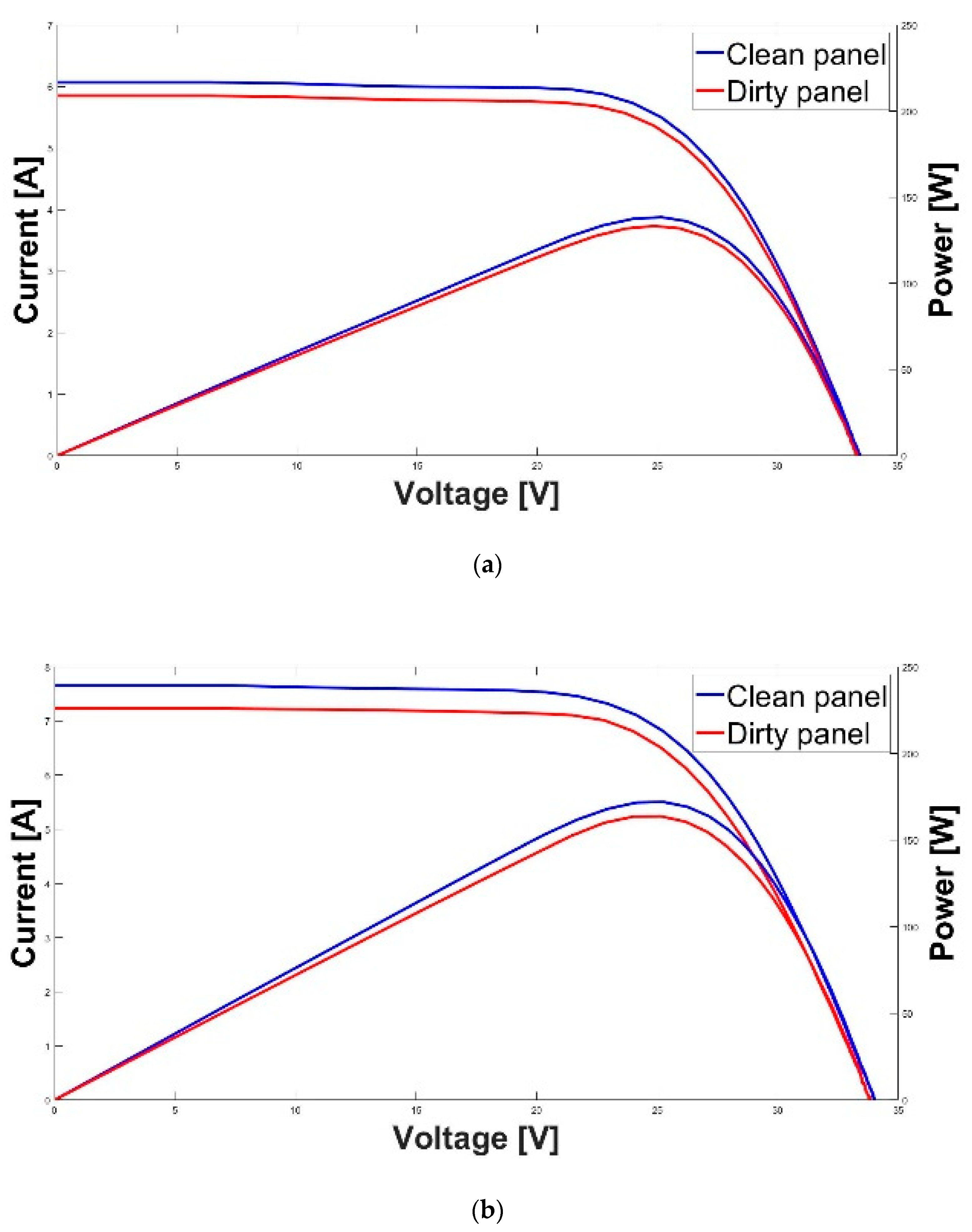
To begin with, a pair of curves taken from clear days in different months are presented to analyze the variation in the characteristic parameters throughout the acquisition campaign. Figure 3 corresponds to the curves measured on 17 January and 14 March, where the x-axis shows the voltage, the primary y-axis the short circuit current and the y-axis seconds the panel power.
Comparing the two images over time, one can see that the amount of dust deposition has increased, making the difference between the characteristic parameters for March greater than in January even though production was higher due to the higher incident radiation levels. These images also show how the short circuit current (a current equal to zero) is the parameter most affected by the dust deposition on the PV panels. In fact, this is the parameter used in several similar studies.
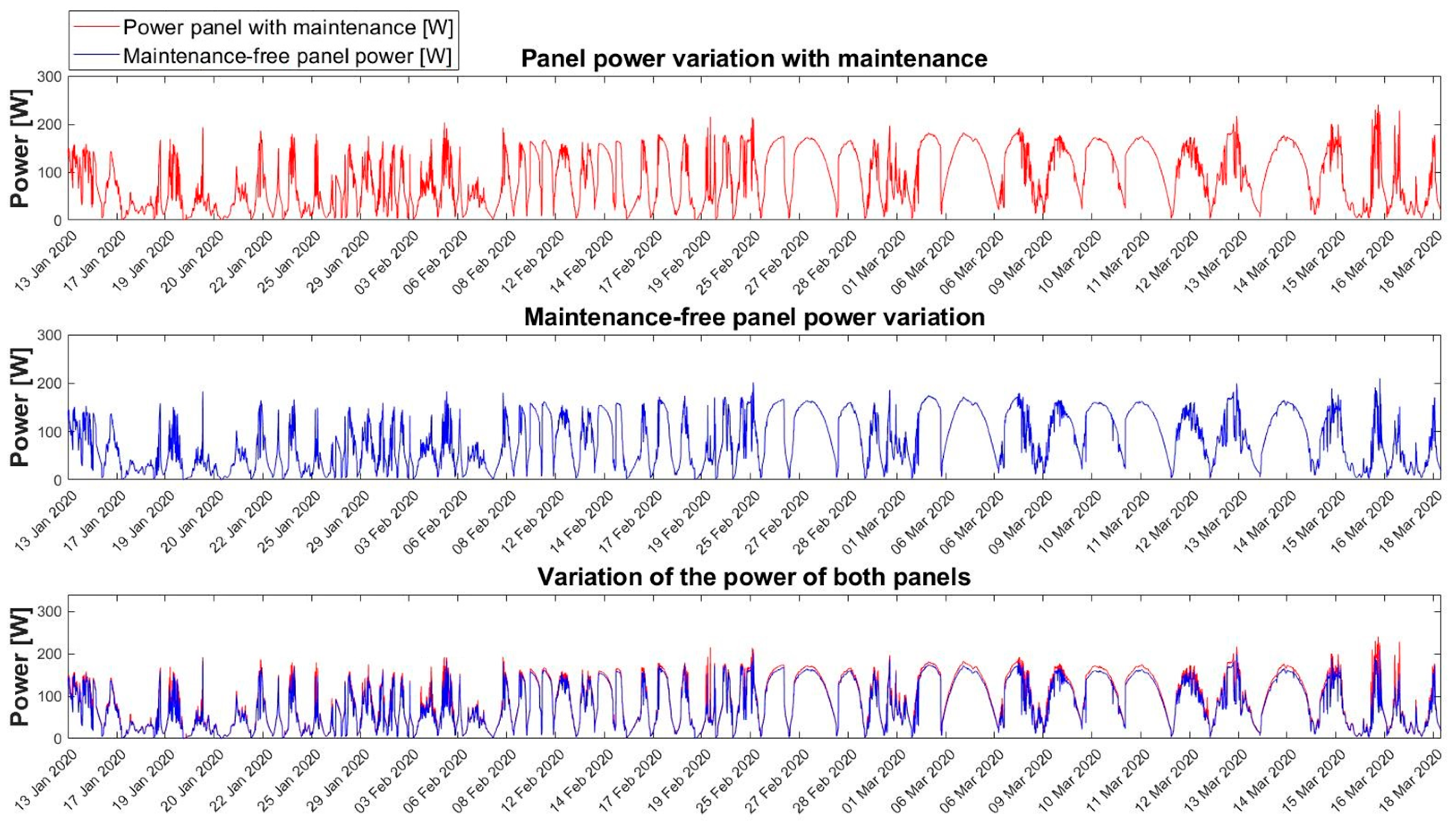
The graphs in Figure 4 represent the maximum power of the PV panels (y-axel) studied at each moment (x-axel). The upper graph shows the variation in power of the panel with maintenance whereas the middle graph shows the variation in power of the panel without maintenance over the measurement campaign. In the lower graph, the two preceding graphs have been superimposed to show the difference in power existing between the two panels. At all times, the power of the panel with maintenance was higher than that for the panel without maintenance. It can also be seen how the power difference over time becomes greater as dirt accumulates; this is due to the lack of maintenance and heavy rainfall.
In this work, clear-day values were used since they are more suitable for calculating the variation in power loss; hence, there will be fewer errors in the final result.
3.2. Dust Losses
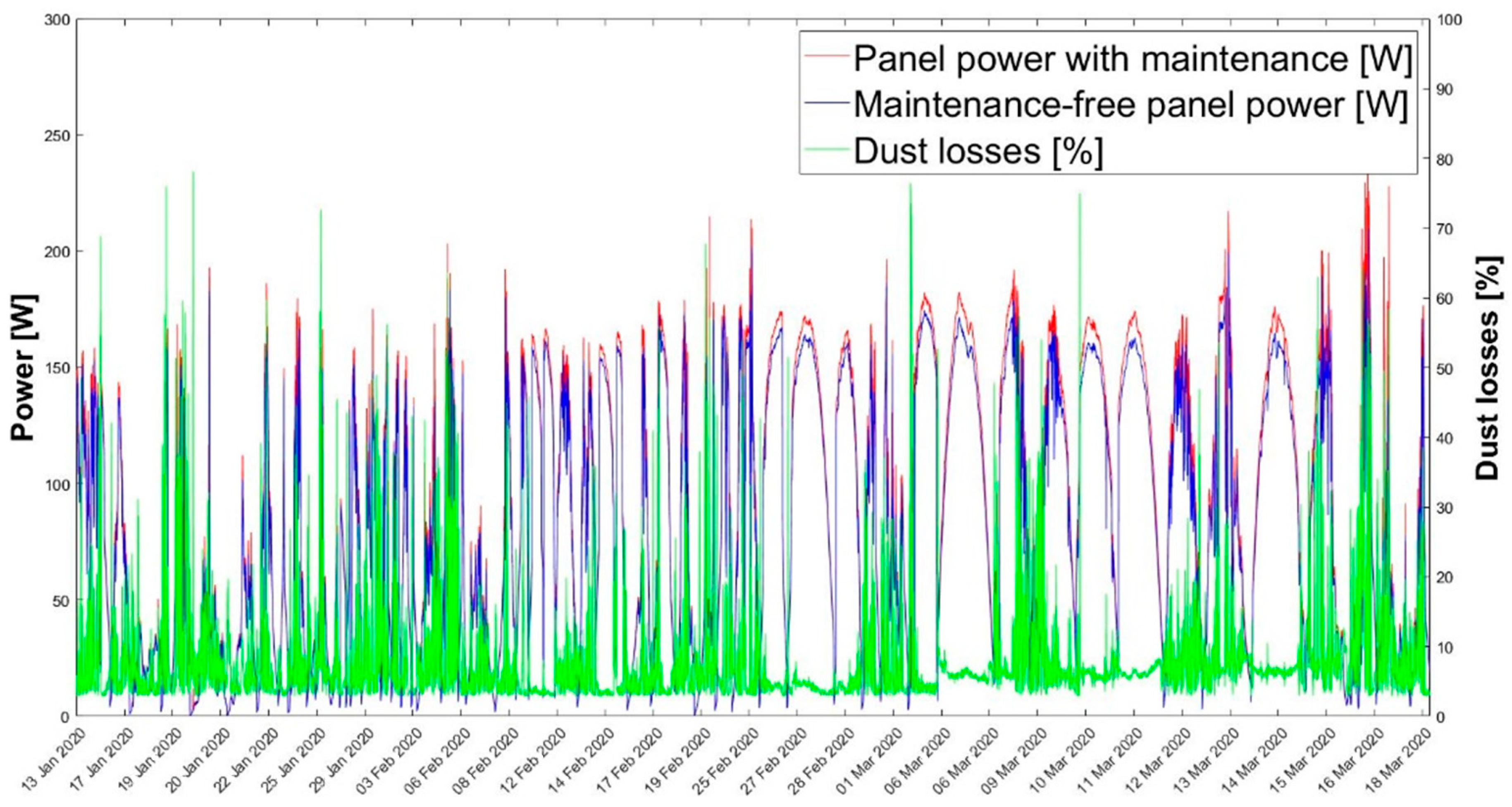
Once the power of each panel is known, the power loss can be determined according to Equation (1). As can be seen in Figure 5, the variation in reduced power associated with dust pollution has noise in the sections where the incident radiation is low, where the x-axis represents the measurement time, the primary y-axis the power and the secondary y-axis the dust losses.
This noise is due to integrating the error of the different signals required to calculate the power loss associated with dust deposition. As previously stated, these values correspond mainly to the times when the received radiation is low. At those moments, the determination of the different electrical parameters on which the power loss calculation is based, has been less precise. Consequently, we performed a filtering to eliminate the sections in which the variable contained noise.
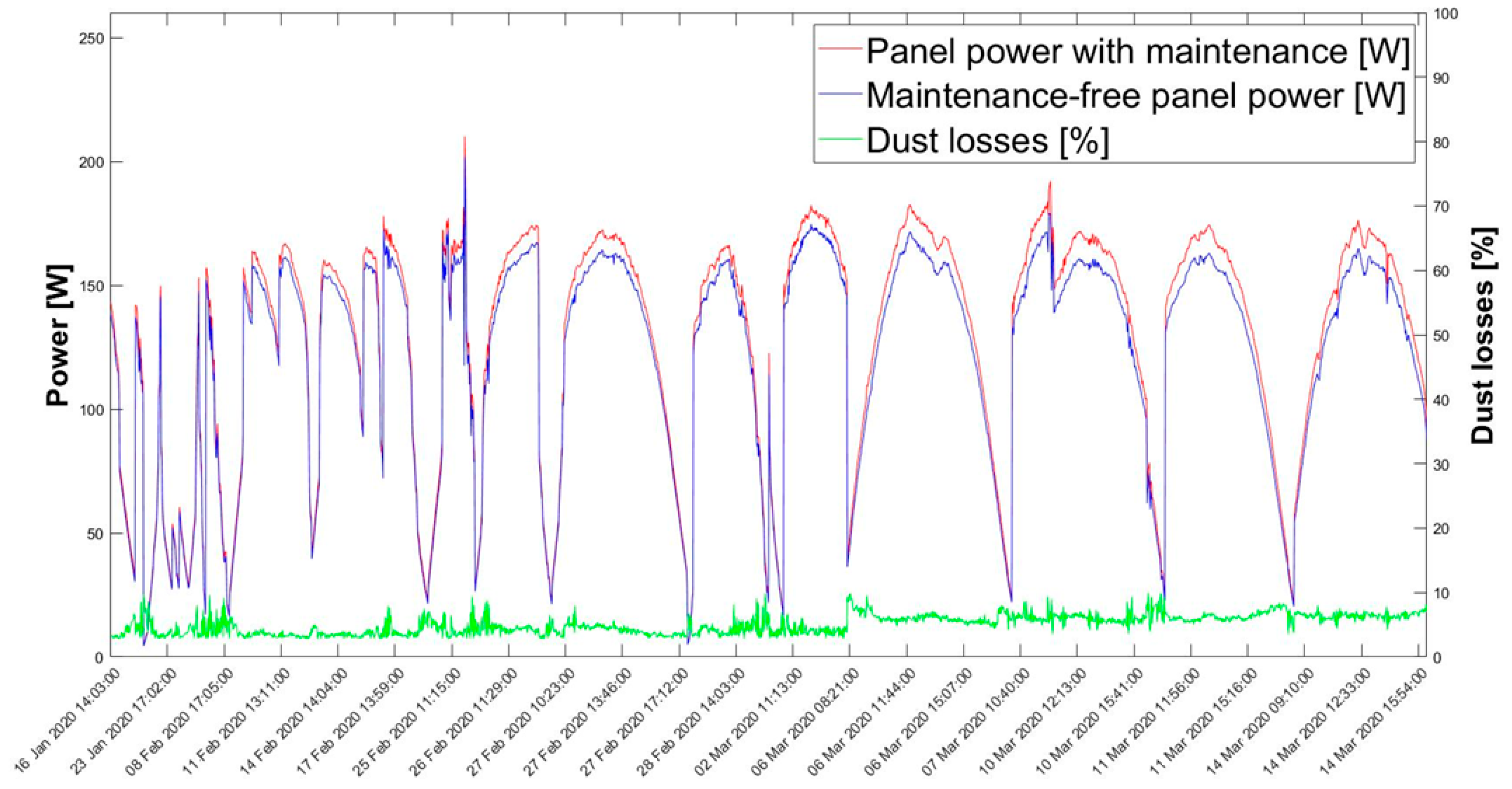
Once the moments in the calculated production losses variable containing noise were discarded, the graph in Figure 6 was obtained.
As can be observed, on most of the days in January and early February, there were cloud passages that made it difficult to determine the loss factor associated with dust contamination. However, on the remaining days, there are losses with lower peaks that make it possible to calculate a representative loss factor for the period under study.
The following average production soiling factors were obtained for each month, and for the entire study period: as shown in Table 4, the factor increases with time, especially when there is no rainfall. The reduction factor for the month of March is the most precisely calculated since it is a month in which most of the days studied were clear, allowing it to be uniformly calculated. In addition, 11 June was one of the days when the sky was clear. After analyzing this day, it was observed that, due to the conditions in Almería, the panels were cleaned periodically due to rainfall, so the losses did not accumulate and, therefore, an annual adjustment cannot be made using the months analyzed.
Once the variation in the loss factor from dust was determined, the variation in the different recorded meteorological variables were represented, together with the power losses, to analyze the possible dependence between them.
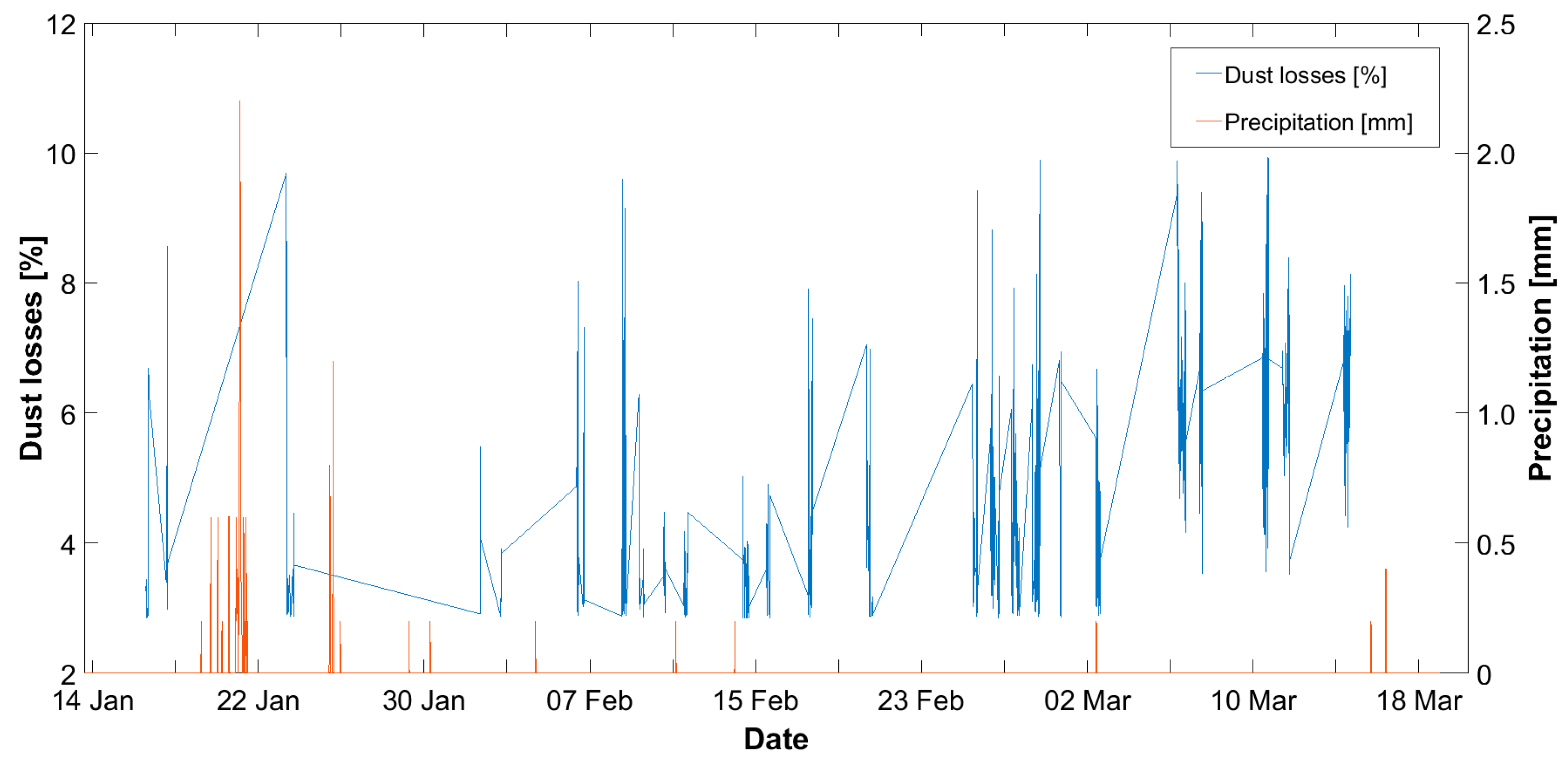
The rain episodes that occurred over the measurement campaign were represented in order to analyze their influence on the variation in the determined power losses (Figure 7). In this graph, dust losses (primary y-axis) and precipitation (secondary y-axis) are represented against time (x-axis).
The most important rains fell at the beginning of January, coinciding with the days when there was sky cover. At those moments, the signal noise is extremely high so most of the records for these days have been filtered out. Some rain episodes were also observed during the month of March although these were episodes in which little rain fell, having practically no repercussion on the variation in power loss.
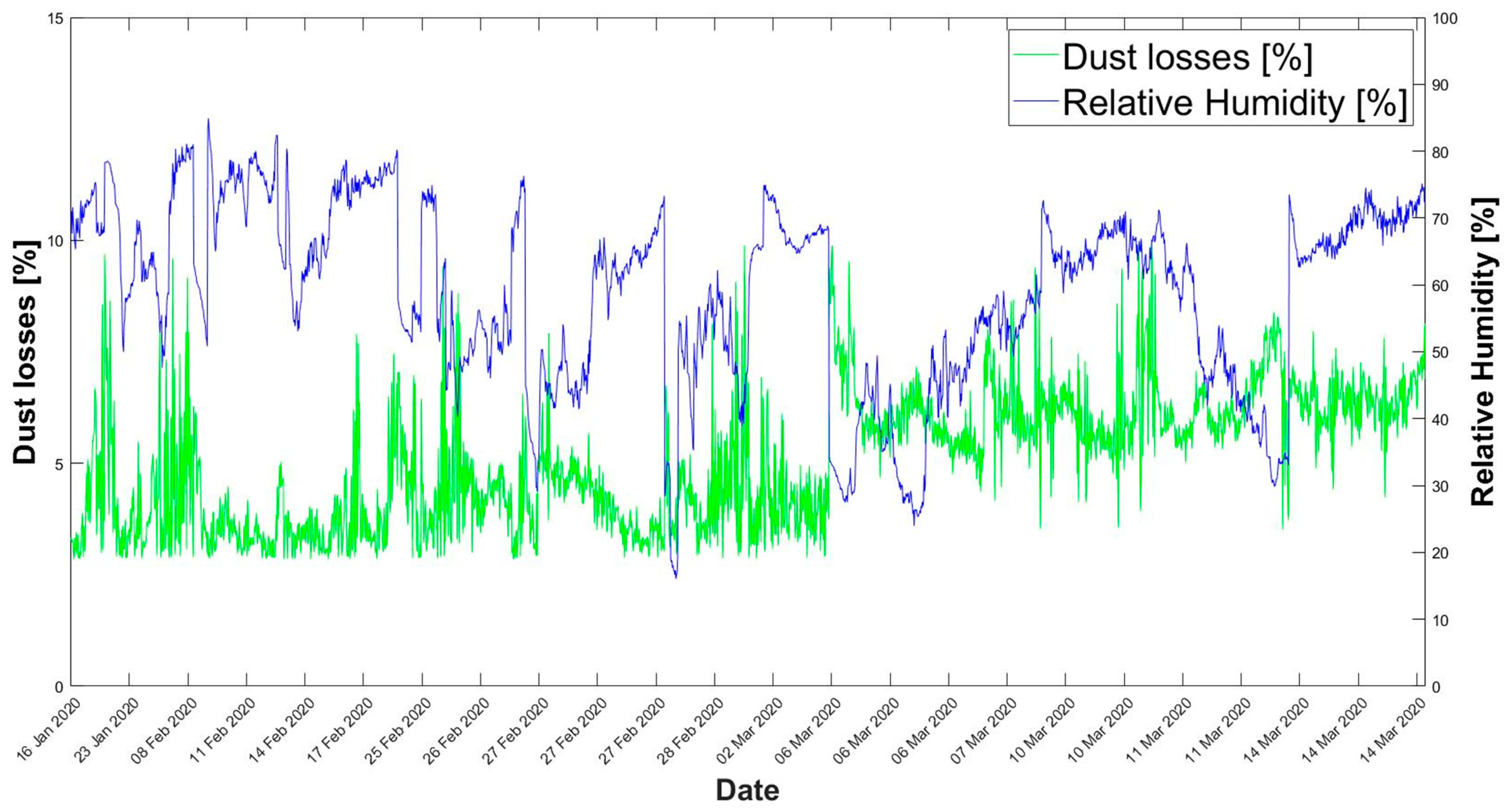
The dust losses (primary y-axis) and relative humidity (secondary y-axis) are shown against time (x-axis) in Figure 8.
A priori, no clear pattern can be observed between the two variables, although it can be stated that, at times when humidity is high due to rainfall (Figure 7), dust losses are high; indeed, when there is rain, optimal conditions do not exist for determining the dust losses of the panels.
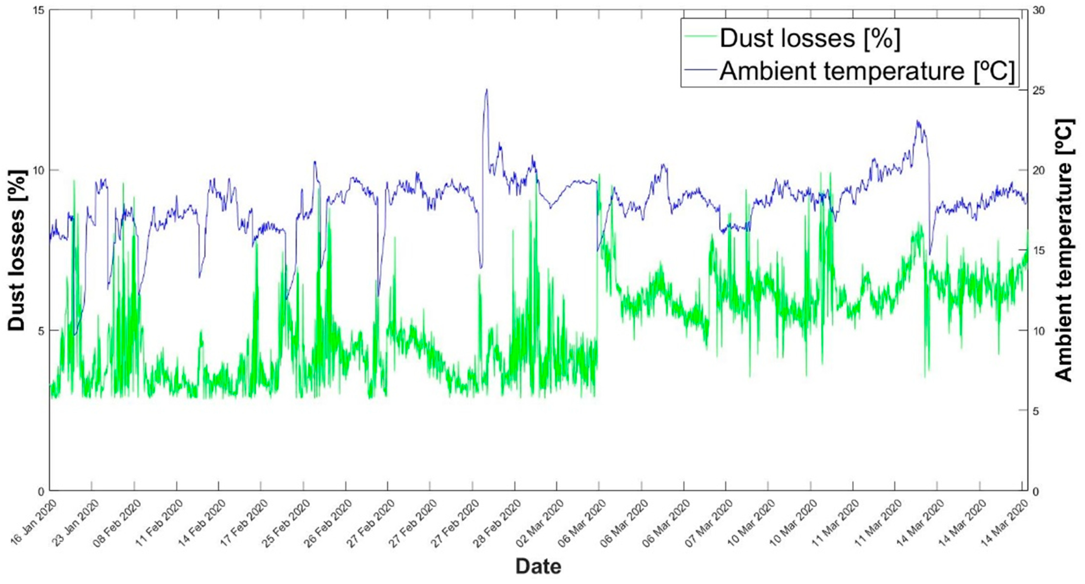
Figure 9 shows the dust losses (primary y-axis) and the ambient temperature (secondary y-axis) in function of time (x-axis). There are probably areas where a common pattern can be seen in the two curves, and one can deduce that there may be some synchronicity between the ambient temperature and the dust loss. Above all, this will occur based on the time of day, so the irradiance in the array plane is probably also representative.
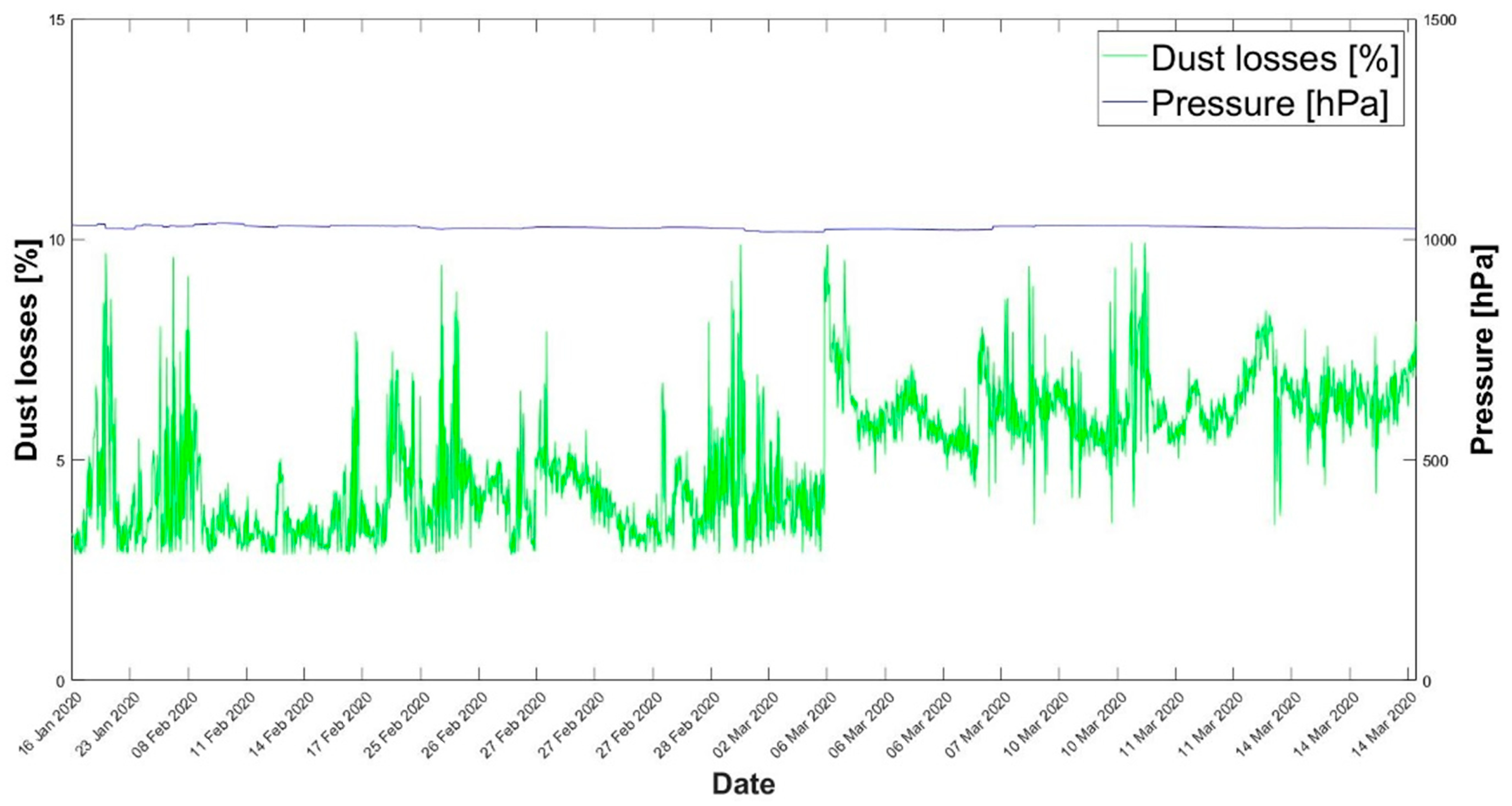
Figure 10 compares the dust losses (primary y-axis) and the pressure (secondary y-axis) in function of time (x-axis). Pressure is a characteristic site variable that does not change over time so a clear relationship between the two variables cannot be established.
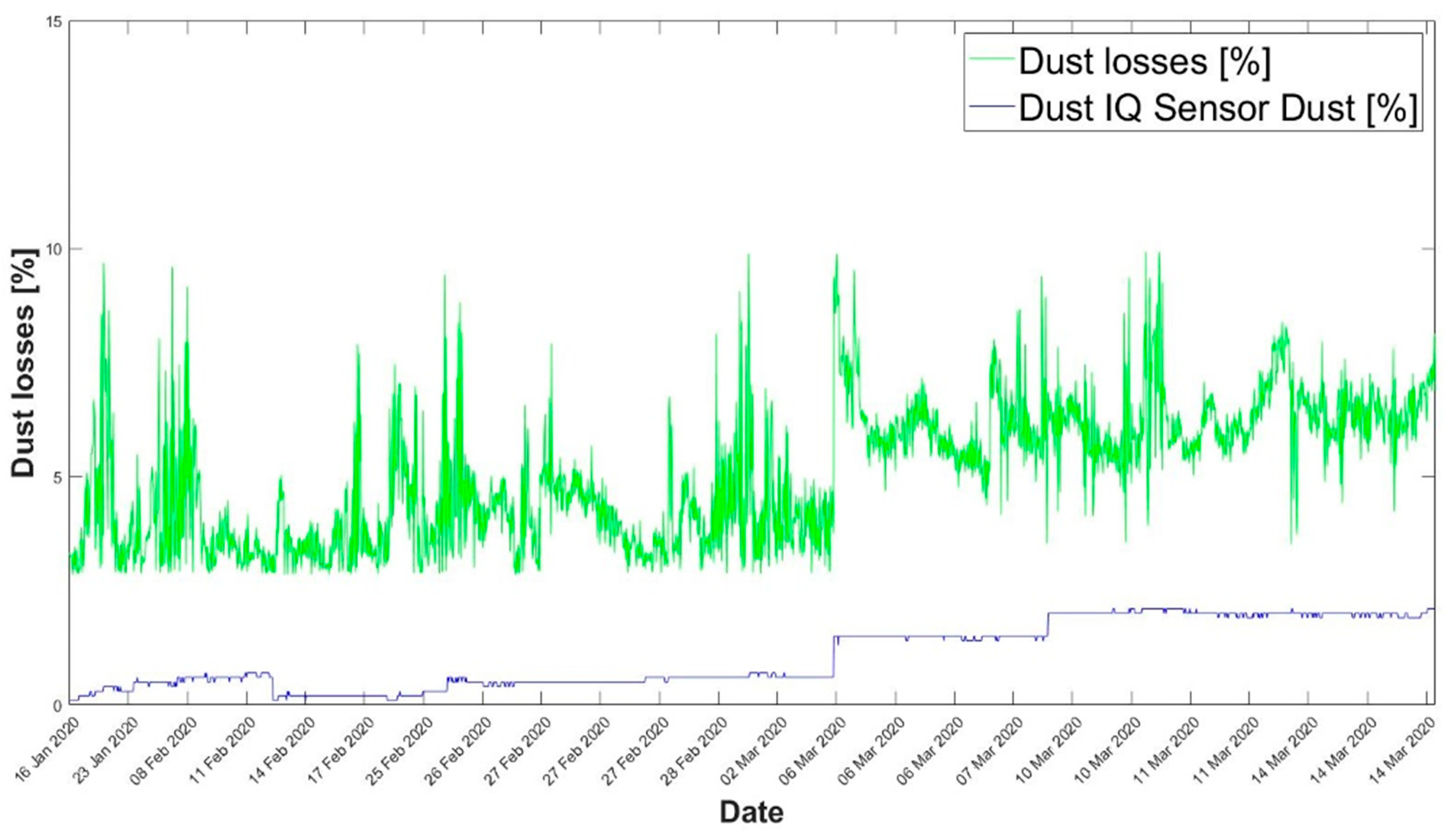
Figure 11 shows the variation in accumulated dust recorded by the experimental facility’s dust sensor (Dust IQ) and the dust losses determined according to the methodology set out in this work.
When representing both variables, it can be seen that significant differences in the magnitude of the sensor measurements are maintained. However, one can observe a similar trend to that in the losses determined.
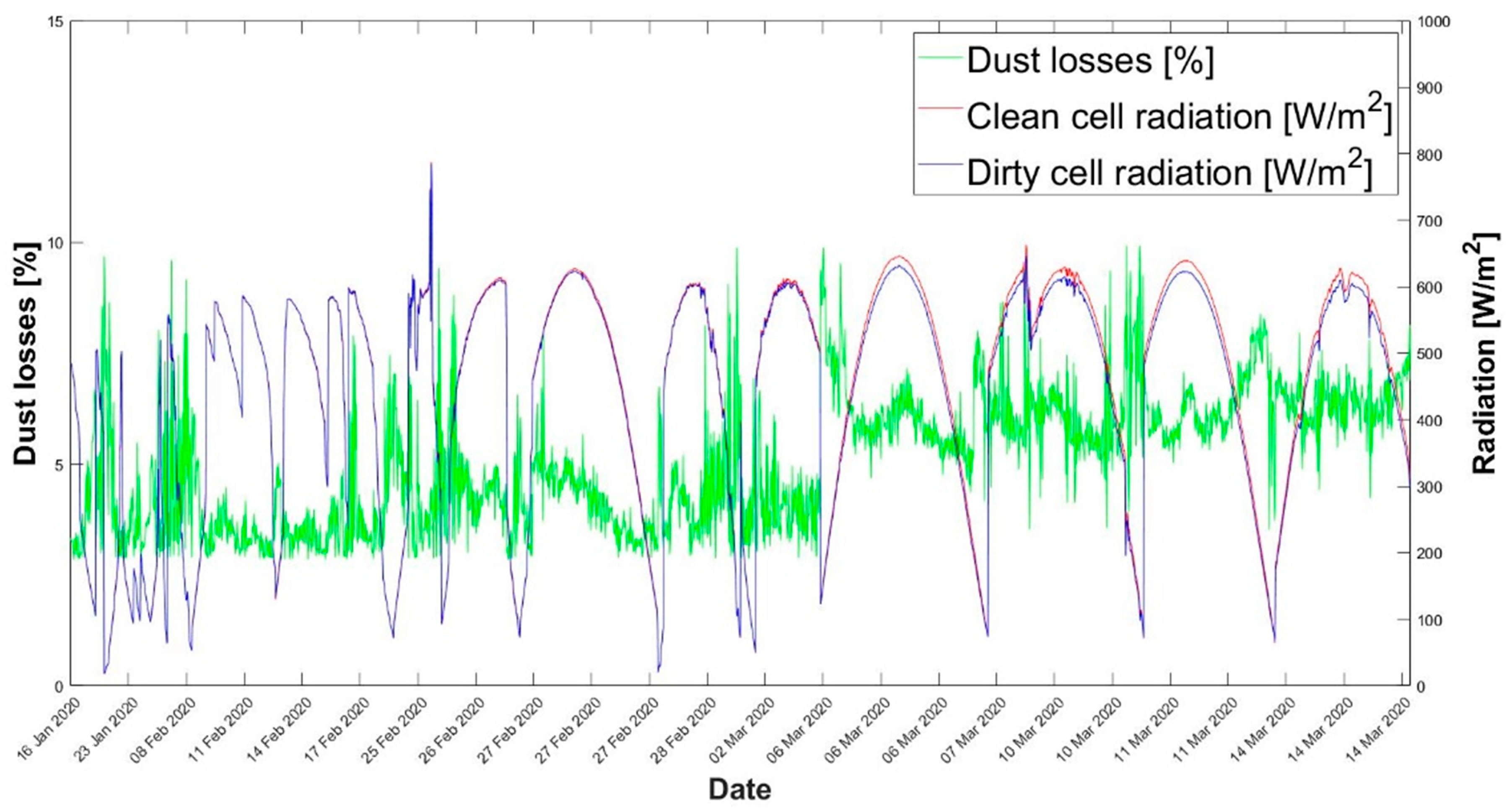
Figure 12 shows the variation in the dust losses determined (primary y-axis) and the radiation of the calibrated cell when maintenance is carried out (secondary y-axis). This graph demonstrates that which has previously been commented on: that the reduced production factor determination is more precise on clear days.
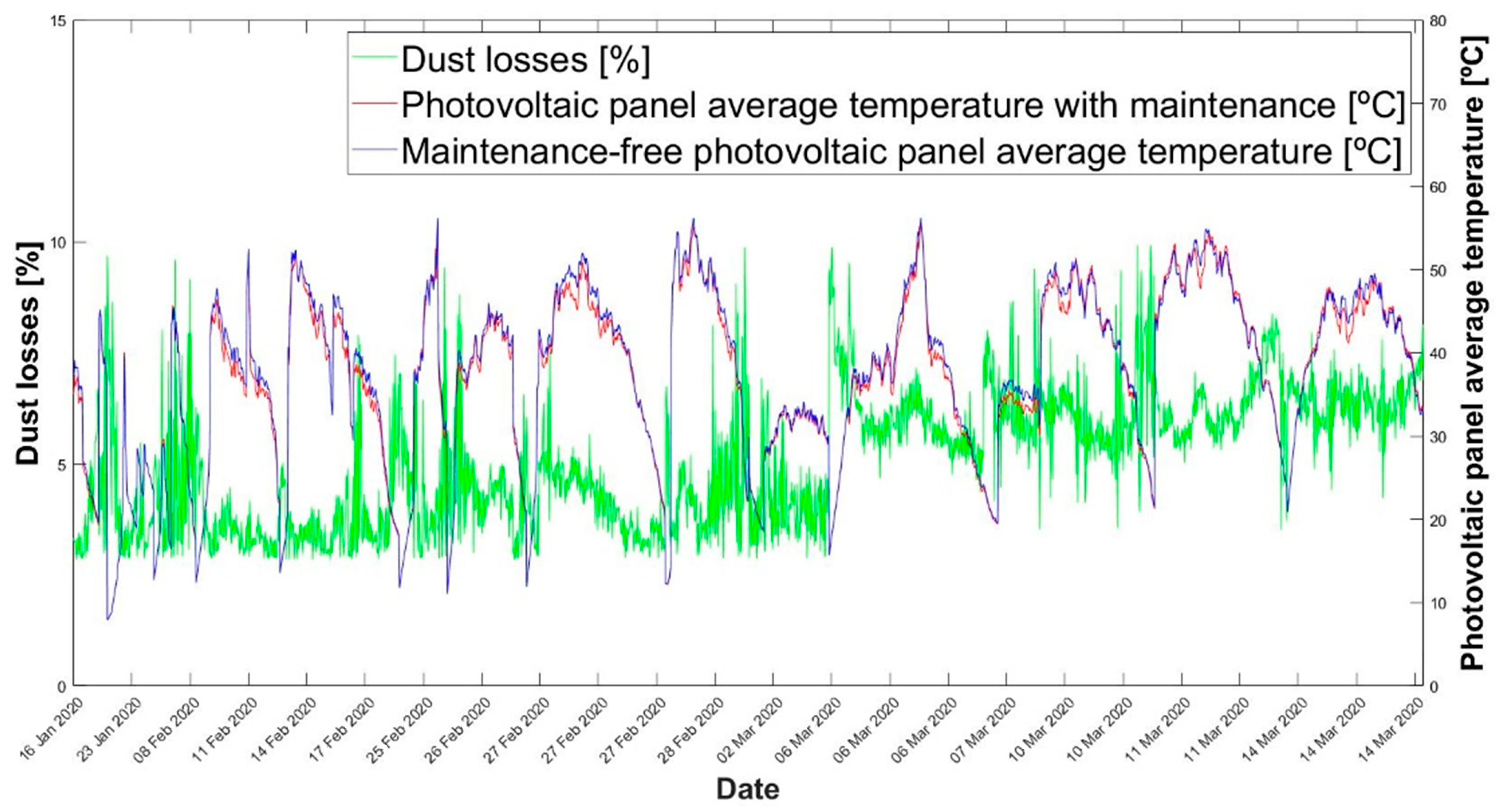
Finally, Figure 13 shows the dust losses (primary y-axis) and the average temperature determined for each panel based on the data provided by the resistive sensors installed in each panel (secondary y-axis) against time (x-axis).
As can be seen, the average temperature of the PV panel that received no maintenance was higher than that for the PV panel that did receive maintenance. This may be due to the generation of small hot spots caused by the non-uniform incidence of radiation on the panel with accumulated dust.
3.3. Solar Energy Research Center (CIESOL) Plant Simulation (9 kWp)
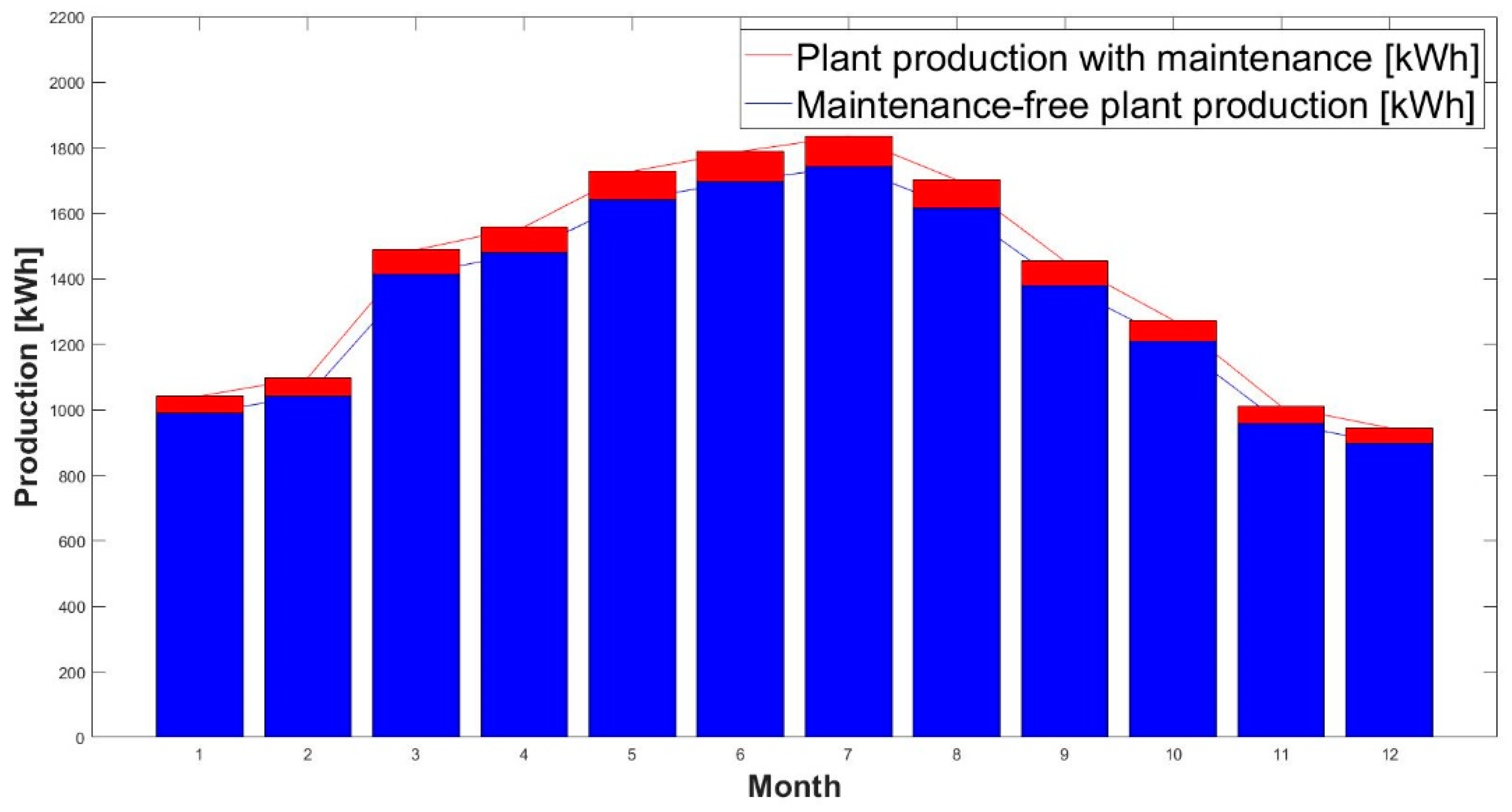
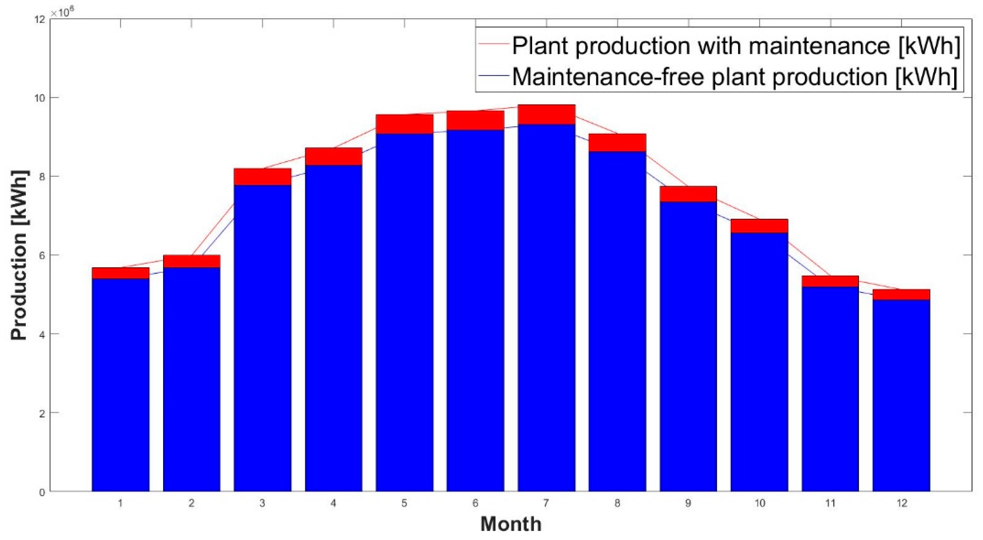
Figure 14 shows the results obtained when simulating the 9 kWp CIESOL plant in the two scenarios proposed in this paper. The monthly output, without taking into account the dust losses of the CIESOL plant in SAM, is shown in red. In blue, the resulting production is shown if the average reduced production factor from dust (calculated in the measurement campaign) were applied. In this case, the difference in production between the two proposed scenarios is not significant.
Based on the results obtained for both scenarios, and with the average monthly values for electricity sales in 2019, the revenues from each scenario are shown in Table 5, where clean and dirty plant production [kWh] shown in the previous figure are presented in the form of columns (2nd and 3rd). The subsequent columns represent the product between the plant production and the average price of the electricity (Table 2) and the final column is the difference between incomes of the clean and dirty plants.
This table breaks down the plant’s production for each of the implemented scenarios along with the monthly revenues generated in each. Additionally, the economic losses that would occur in each month if the plant were not cleaned have been broken down.
The last row summarizes the plant’s income under the different scenarios proposed and the total annual economic loss, which would amount to 41.06€. Hence, the annual economic loss in this case is practically irrelevant.
Figure 15 shows the approximate daily variation in dust losses that would be experienced by a plant in Rumah if it were in an optimally clean condition at the beginning of the year.
It can be seen that, in this region, the percentage of losses due to dust peaks in April, reaching 15%. Its lowest accumulated dust value occurs around July.
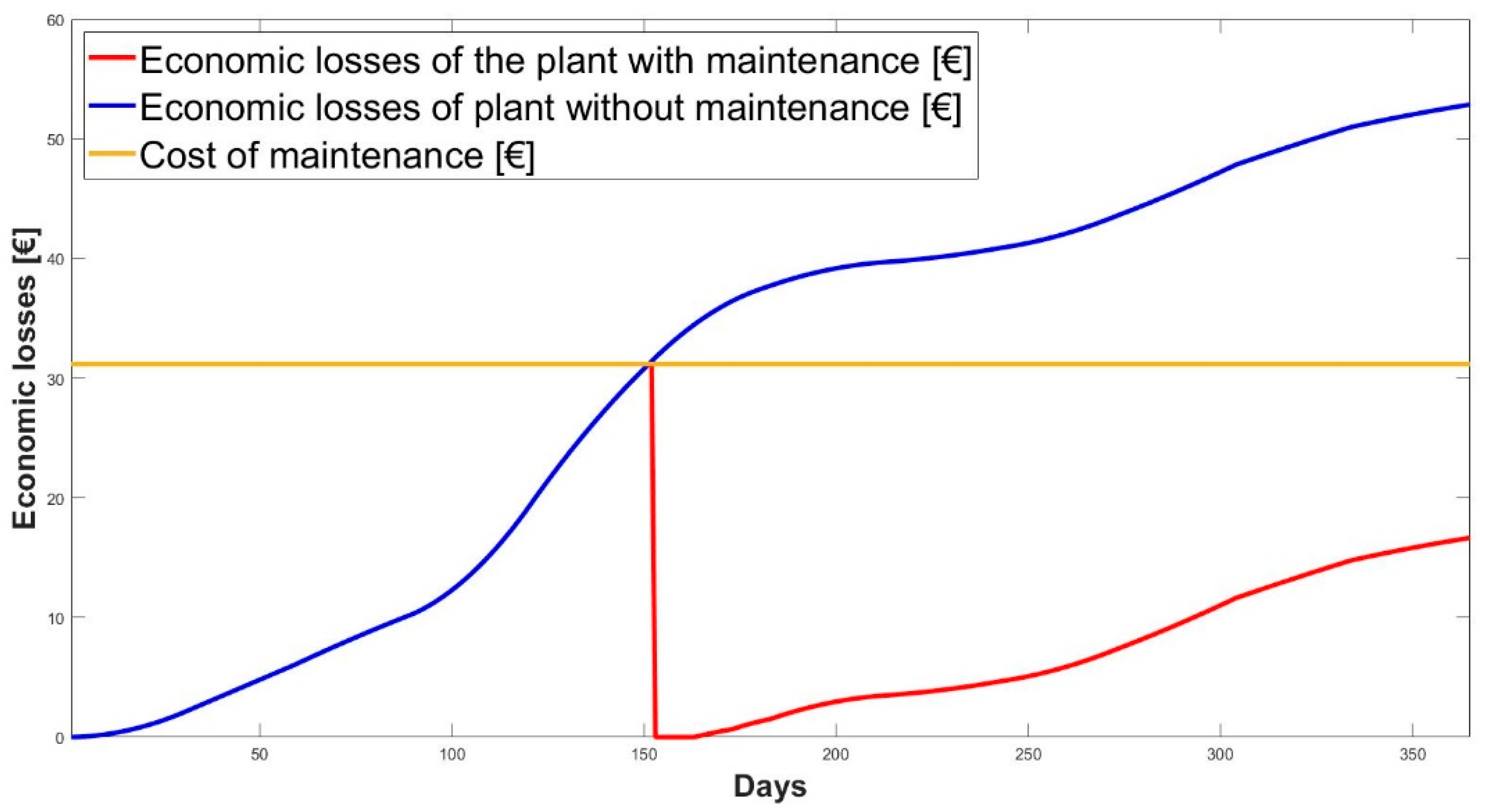
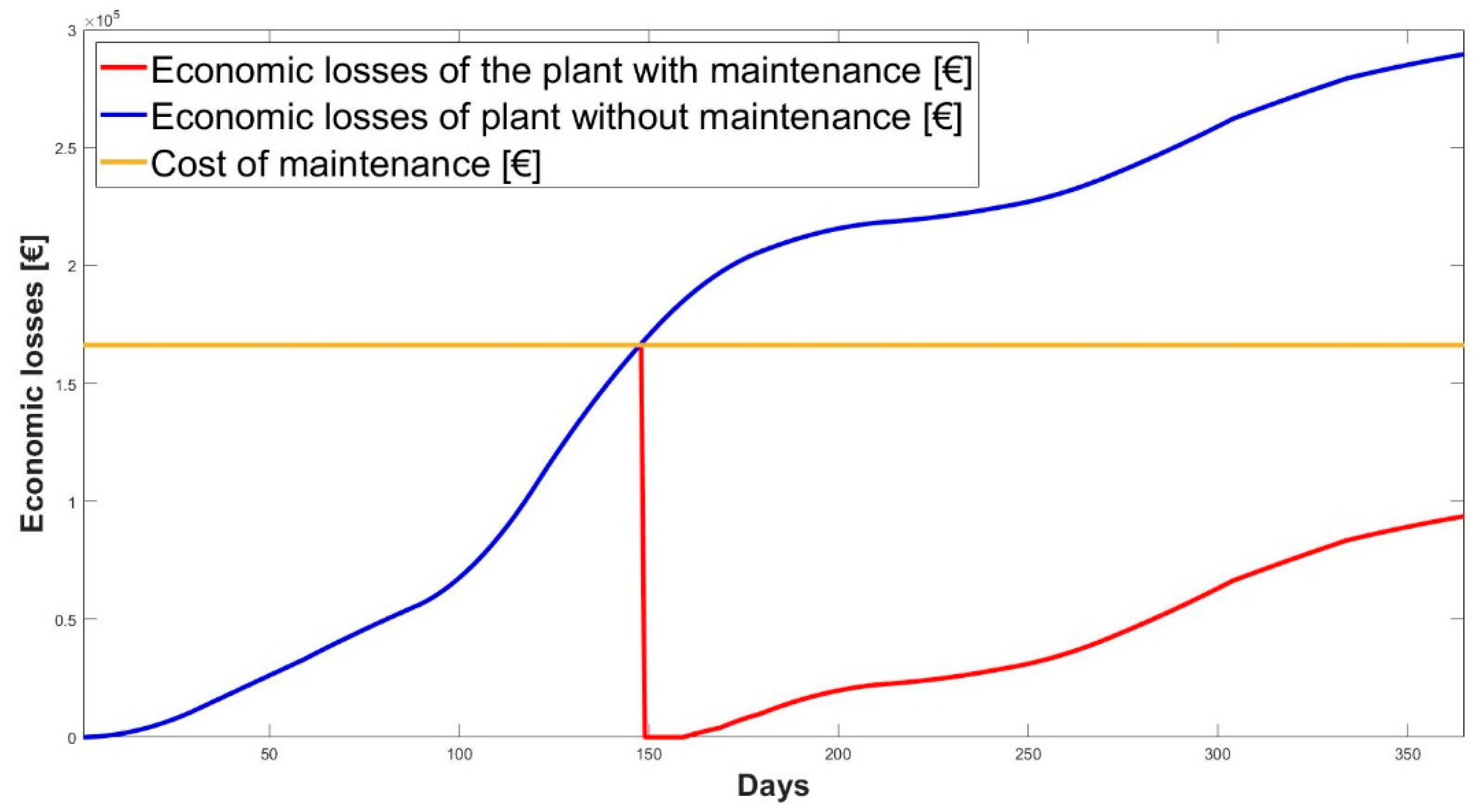
Figure 16 shows the accumulated economic losses for a year with and without maintenance if the production of the CIESOL plant and the losses due to dust recorded in Rumah are taken into account (Figure 15), together with the maintenance cost of the CIESOL plant.
As the figure shows, if maintenance were carried out at this plant according to the methodology described above, it would be necessary to carry out a cleaning on the 152nd day (1 June), as this is the point at which the accumulated losses would exceed the plant cleaning cost. Table 6 shows a breakdown of the losses that would occur in the plant with and without maintenance.
As shown in Table 6, it would not be profitable to apply cleaning based on the methodology described above; this is because, at the end of the year, greater economic losses would be incurred than would be the case if regular maintenance were not carried out.
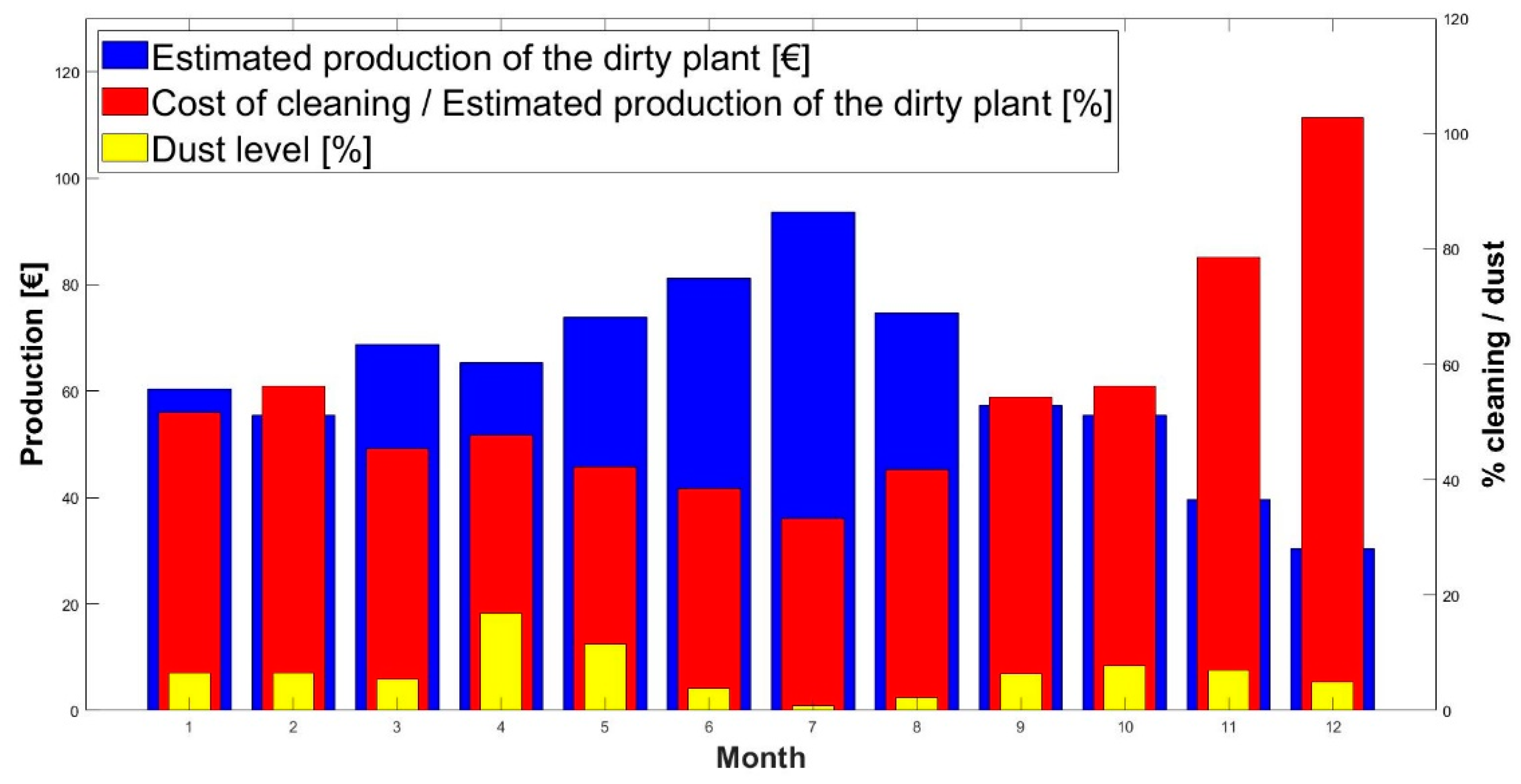
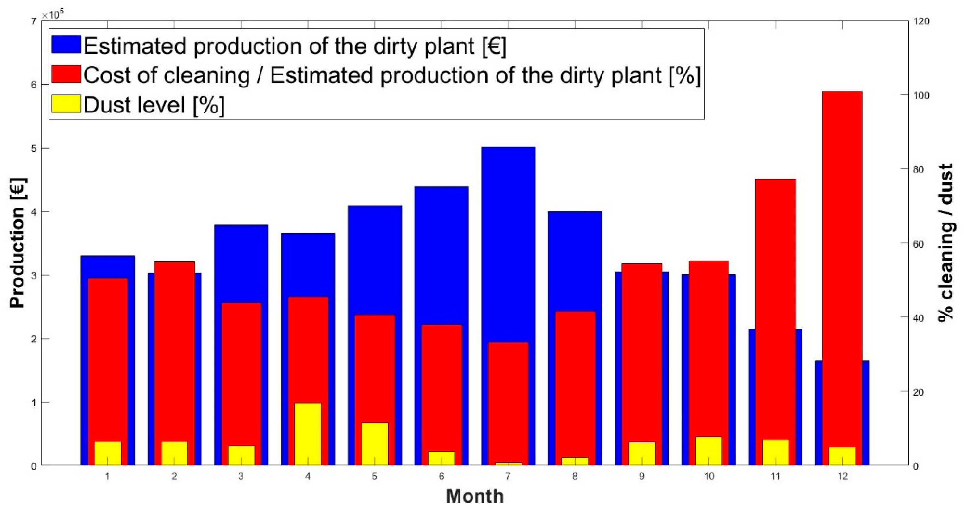
Maintenance would only be profitable if there were higher levels of contamination. Figure 17 shows (in red) the dust level that would have to be reached each month for cleaning to be profitable, and the level of dust (in yellow) according to the methodology explained.
The red bars show the percentage of dust cleaning and the corresponding economic remuneration that would be obtained from the sale of the generated electricity (represented in blue).
To make cleaning profitable, the level of accumulated dust must exceed the proportion of economic remuneration that the cleaning corresponds to. As can be seen in the graph, the highest electricity sales values occur in the summer, so the proportion of cleaning costs is lower at that time. Plant cleaning will be more profitable during these months.
3.4. Simulation of the 1 MWp Plant
Figure 18 shows the monthly production of the 1 MWp plant simulation for the two scenarios presented in this paper.
As the monthly electricity generation at the photovoltaic plant increases, one can observe how the production losses associated with dust pollution become more important, arriving at losses of up to 10 MWh during the months of greatest generation.
Based on the results obtained for the two proposed scenarios, the values in Table 7 are obtained.
In this industrial plant simulation, one can see how the economic losses associated with dust pollution during the months of greatest production amount to 460€. For this plant, the decrease in production due to dust translates into annual losses of 4466.85€, a considerable amount of money.
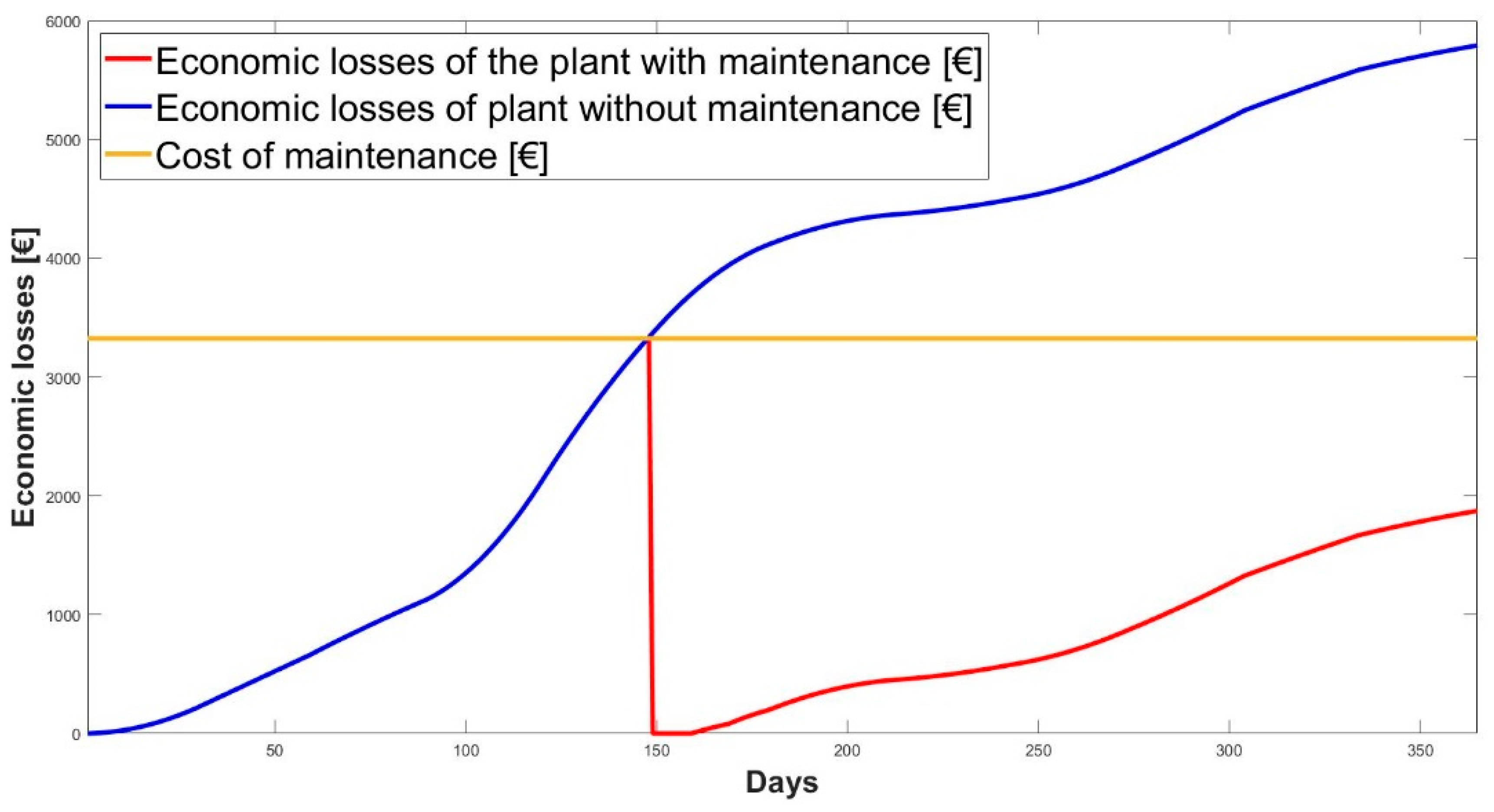
Figure 19 shows the accumulated economic losses over one year, with and without maintenance, together with the maintenance cost of the 1 MWp plant.
If maintenance were carried out at this plant in accordance with the above methodology, it would be necessary to clean it on day 148 (28 May) since this is the point at which the accumulated losses would be greater than the 3326€ that it would cost to clean the plant. Table 8 shows a breakdown of the losses that would be incurred in the plant, with and without maintenance.
As in the case of the CIESOL plant, it would not be profitable to clean based on the methodology set out above, since the total economic losses would amount to 2745€ over the year if the cleaning work were carried out on the scheduled day.
In order for the investment involved in plant cleaning to be profitable, higher dust percentages would have to be present. The percentages of dust required to amortize the economic losses that would result from cleaning the plant are shown (in red) in Figure 20.
One can observe how, in the summer months, the proportion of the cleaning cost in relation to the electricity sales would be greater. However, according to the data on the dust level used, in March the difference between this and the level that would be needed to make it profitable is less; that is to say, according to the data on the reduced production due to dust, it would be more profitable to clean in March as the difference would be smaller.
3.5. Simulation of the 50 MWp Plant
Figure 21 shows the results obtained for the 50 MWp plant for the two scenarios proposed. One can see how the difference in generation between the two scenarios is more notable in the months of greatest production. In this period, monthly production losses of up to 500 MWh would occur.
Table 9 presents the values based on the data obtained for both scenarios.
As one can observe, the economic losses associated with dust pollution for a 50 MWp plant would reach 25,000€ in the months of greatest production. The average soiling observed in the experimental plant would translate to annual losses of 223,342.68€ in a 50 MWp industrial plant.
Figure 22 shows the graphical results of representing the accumulated economic losses over one year, with and without maintenance, together with the maintenance cost of the 50 MWp plant.
As can be seen, if maintenance were carried out at this plant in accordance with the methodology described above, it would be necessary to clean on day 148 (28 May), at which time the accumulated economic losses associated with dust contamination would exceed the plant’s cleaning cost, which amounts to 166,300€.
Table 10 gives a breakdown of the economic losses that would occur in the 50 MWp plant, with and without maintenance.
The cost of cleaning is still too high so cleaning would not be profitable as the total economic losses would amount to 137,330€; this economic loss is more than if the photovoltaic plant were not cleaned.
To achieve a return on the cleaning investment for a plant of this size, contamination levels equal to those described by the red bars in Figure 23 would need to be reached.
4. Conclusions
This work presents a methodology developed to determine the energy and economic losses associated with dust pollution in an area that has an excellent solar resource, but which can be influenced by the presence of dust particles in the atmosphere. This study may serve as a prelude to creating a new plant that can optimally determine profitability based on certain meteorological conditions.
Through the simulations carried out with the System Advisor Model (SAM) tool, we have demonstrated a way of modelling solar plants free of charge. Thanks to this software, which is widely used for plant modelling on a global scale, it has been possible to compare the varying effects of dust deposition on solar plants for a location such as Almería. In addition, these simulations have made it possible to analyze the behavior of different-sized plants that operate using polycrystalline silicon technology in their PV panels.
A method has been presented to optimize the cleaning interval of a photovoltaic plant that could be used once the variation in annual dust pollution has been determined. These results can be utilized for sites on the Mediterranean coast with similar characteristics to those of Almería, making it possible to optimize the solar resource and water usage, given that the latter is a scarce resource at some of the sites possessing the greatest solar potential.
After carrying out the optimal cleaning interval analysis, one can conclude that, for cleaning to be profitable, the percentage of losses caused by dirt deposition must exceed the percentage of economic losses that the resultant maintenance work would entail.
A methodology has been presented for determining the power losses associated with dust deposition on PV panels using an economic curve acquisition system. The average soiling factor determined for the Almería region during the winter and summer months is 5.07%. Furthermore, it has been observed that dust pollution varies according to the atmospheric variables in the area, a result of the prevailing meteorological conditions. Finally, the importance of carrying out periodic cleaning work on industrial PV plants has been shown, although dust deposition in 9 kWp plants might lead to annual economic losses of just 40€, in 1 MWp and 50 MWp plants, economic losses of over 4400€ and 200,000€, respectively, could be incurred. In this study, the levels of dust used for the calculations did not reach the percentages required to make cleaning profitable in any month; nonetheless, the methodology can be used by plant operators to determine whether cleaning would be profitable once the annual variation in reduced production associated with dust contamination is known for the site where the photovoltaic plant is located.
It should also be taken into account that, as the capacity and area of the photovoltaic plant increases, the possibility arises of establishing agreements with maintenance companies that reduce the prices of plant cleaning. Under such conditions, where the plant cleaning cost is reduced, the potential return would be even higher than that proposed by the different articles referred to in the literature.
One can conclude from these results that, even in environments with a high level of dust, photovoltaic plants might be able to carry out their activity without the need for maintenance given that, from an economic standpoint, the activity is still profitable, although to a lesser degree, as demonstrated in the results section.
Finally, one should bear in mind that, although cleaning is not profitable according to these calculations, dust deposition creates hot spots on the photovoltaic panels which might lead to them being damaged.
Author Contributions
Conceptualization, J.A.-M. and F.R.M.; methodology, J.A.-M., F.R.M. and N.M.-C.; software, F.R.M. and J.P.; validation, J.A.-M., N.M.-C. and F.J.B.; formal analysis, J.A.-M.; investigation, J.A.-M., F.R.M., J.P.; resources, J.A.-M.; data curation, F.R.M.; writing—original draft preparation, J.A.-M. and F.R.M.; writing—review and editing, J.A.-M.; visualization, J.A.-M. and F.R.M.; supervision, J.A.-M.; project administration, F.J.B.; funding acquisition, F.J.B. All authors have read and agreed to the published version of the manuscript.
Funding
This research received no external funding.
Acknowledgments
The authors would like to acknowledge the support given by the Spanish Ministry of the Economy, Industry and Competitiveness, “PVCastSoil” project N° ENE2017-83790-C3-1-2-3-R, in collaboration with the European Regional Development Fund”.
Conflicts of Interest
The authors declare no conflict of interest.
References
- Shafiei, S.; Salim, R.A. Non-renewable and renewable energy consumption and CO2 emissions in OECD countries: A comparative analysis. Energy Policy 2014, 66, 547–556. [Google Scholar] [CrossRef] [Green Version]
- Thirugnanasambandam, M.; Iniyan, S.; Goic, R. A review of solar thermal technologies. Renew. Sustain. Energy Rev. 2010, 14, 312–322. [Google Scholar] [CrossRef]
- Menéndez, J.; Loredo, J. Economic feasibility of developing large scale solar photovoltaic power plants in Spain. E3S Web Conf. 2019, 122, 02004. [Google Scholar] [CrossRef]
- Honrubia-Escribano, A.; Ramirez, F.J.; Gómez-Lázaro, E.; Garcia-Villaverde, P.M.; Ruiz-Ortega, M.J.; Parra-Requena, G. Influence of solar technology in the economic performance of PV power plants in Europe. A comprehensive analysis. Renew. Sustain. Energy Rev. 2018, 82, 488–501. [Google Scholar] [CrossRef]
- Martín-Martínez, S.; Cañas-Carretón, M.; Honrubia-Escribano, A.; Gómez-Lázaro, E. Performance evaluation of large solar photovoltaic power plants in Spain. Energy Convers. Manag. 2019, 183, 515–528. [Google Scholar] [CrossRef]
- John, J.J.; Warade, S.; Tamizhmani, G.; Kottantharayil, A. Study of Soiling Loss on Photovoltaic Modules With Artificially Deposited Dust of Different Gravimetric Densities and Compositions Collected From Different Locations in India. IEEE J. Photovolt. 2016, 6, 236–243. [Google Scholar] [CrossRef]
- Micheli, L.; Deceglie, M.G.; Muller, M. Predicting photovoltaic soiling losses using environmental parameters: An update. Prog. Photovolt. Res. Appl. 2019, 27, 210–219. [Google Scholar] [CrossRef]
- Conceição, R.; Silva, H.G.; Mirão, J.; Gostein, M.; Fialho, L.; Narvarte, L.; Collares-Pereira, M. Saharan dust transport to Europe and its impact on photovoltaic performance: A case study of soiling in Portugal. Sol. Energy 2018, 160, 94–102. [Google Scholar] [CrossRef]
- ADRASE. Acceso a Datos de Radiación Solar de España; ADRASE: Madrid, Spain, 2020. [Google Scholar]
- Alonso-Montesinos, J.; Barbero, J.; Polo, J.; López, G.; Ballestrín, J.; Batlles, F.J. Impact of a Saharan dust intrusion over southern Spain on DNI estimation with sky cameras. Atmos. Environ. 2017, 170, 279–289. [Google Scholar] [CrossRef]
- SIAR. Consultas Avanzadas. 2020. Available online: http://eportal.mapa.gob.es/websiar/SeleccionParametrosMap.aspx?dst=1 (accessed on 4 September 2020).
- OMIE. Precio del Mercado Diario Mibel-2019. 2020. Available online: https://www.omie.es/es (accessed on 25 September 2020).
- Baras, A.; Jones, R.; Alqahtani, A.; Alodan, M.; Abdullah, K. Measured soiling loss and its economic impact for PV plants in central Saudi Arabia. In Proceedings of the 2016 Saudi Arabia Smart Grid (SASG), Jeddah, Saudi Arabia, 6–8 December 2016. [Google Scholar]
- Al-Housani, M.; Bicer, Y.; Koç, M. Experimental investigations on PV cleaning of large-scale solar power plants in desert climates: Comparison of cleaning techniques for drone retrofitting. Energy Convers. Manag. 2019, 185, 800–815. [Google Scholar] [CrossRef]
- Conversor XE. Conversor XE. 2020. Available online: https://www.xe.com/es/currencyconverter/ (accessed on 28 September 2020).
Figure 1.
Monitored experimental installation.

Figure 2.
Scenarios proposed for evaluating the production difference.

Figure 3.
Curves obtained at local time: (a) on 17 January at 13:56 (clean module) and at 13:55 (dirty module); (b) on 14 March at 12:05 (clean module) and at 12:06 (dirty module).
Figure 3.
Curves obtained at local time: (a) on 17 January at 13:56 (clean module) and at 13:55 (dirty module); (b) on 14 March at 12:05 (clean module) and at 12:06 (dirty module).

Figure 4.
Representation of the power variation in the two panels studied along with the filtered values.
Figure 4.
Representation of the power variation in the two panels studied along with the filtered values.

Figure 5.
Variation in power and power loss.

Figure 6.
Variation in production loss during the measurement campaign.

Figure 7.
Effect of rainfall on the variation in production loss during several months.

Figure 8.
Variation in production loss associated with the calculated dust and relative humidity at the experimental plant during the measurement campaign.
Figure 8.
Variation in production loss associated with the calculated dust and relative humidity at the experimental plant during the measurement campaign.

Figure 9.
Variation in the production loss associated with dust and the ambient temperature in the experimental plant during the measurement campaign.
Figure 9.
Variation in the production loss associated with dust and the ambient temperature in the experimental plant during the measurement campaign.

Figure 10.
Variation in the production loss associated with dust and the pressure at the experimental plant during the measurement campaign.
Figure 10.
Variation in the production loss associated with dust and the pressure at the experimental plant during the measurement campaign.

Figure 11.
Variation in the production loss associated with dust and the dust accumulated in the environment around the experimental plant during the measurement campaign.
Figure 11.
Variation in the production loss associated with dust and the dust accumulated in the environment around the experimental plant during the measurement campaign.

Figure 12.
Variation in the production loss associated with dust and the incident radiation at the experimental plant during the measurement campaign.
Figure 12.
Variation in the production loss associated with dust and the incident radiation at the experimental plant during the measurement campaign.

Figure 13.
Variation in the production loss associated with dust and the average temperature of the photovoltaic panels during the measurement campaign.
Figure 13.
Variation in the production loss associated with dust and the average temperature of the photovoltaic panels during the measurement campaign.

Figure 14.
Variation in production at the Solar Energy Research Center (CIESOL) plant (9 kWp).

Figure 15.
Approximate variation in daily dust losses.

Figure 16.
Optimal cleaning interval for the CIESOL plant (9 kWp) from an economic standpoint.

Figure 17.
Representation of the minimum percentage of dust required to make cleaning the CIESOL plant profitable (9 kWp).
Figure 17.
Representation of the minimum percentage of dust required to make cleaning the CIESOL plant profitable (9 kWp).

Figure 18.
Variation in production at the 1 MWp plant.

Figure 19.
Optimal cleaning interval for the 1 MWp plant from an economic standpoint.

Figure 20.
Representation of the minimum dust percentage required to make cleaning the 1 MWp plant profitable.
Figure 20.
Representation of the minimum dust percentage required to make cleaning the 1 MWp plant profitable.

Figure 21.
Variation in production at the 50 MWp plant.

Figure 22.
Optimal cleaning interval for the 50 MWp plant from an economic standpoint.

Figure 23.
Representation of the minimum percentage of dust required to make the cleaning of the 50 MWp plant profitable.
Figure 23.
Representation of the minimum percentage of dust required to make the cleaning of the 50 MWp plant profitable.


Table 1.
Plant configuration.
| Plant | CIESOL’s 9 kWp Plant | 1 MWp Plant | 50 MWp Plant |
|---|---|---|---|
| No. of sublines | 1 | 4 | 4 |
| No. of rows per subway | 3 | 56 | 2800 |
| No. of panels in series per row | 14 | 20 | 20 |
| Plant power | 9324 Wp | 0.99456 MWp | 49.728 MWp |
| Number of inverters per subline | 3 (1 for each branch) | 1 | 50 |
Table 2.
Average monthly price obtained from the daily sales price for 2019 in Spain and the best-fit loss coefficients per month for the polycrystalline technology.
Table 2.
Average monthly price obtained from the daily sales price for 2019 in Spain and the best-fit loss coefficients per month for the polycrystalline technology.
| Month | Average Monthly Price [€/MWh] | a Coefficient [per hour × 10−5] |
|---|---|---|
| 1 | 61.99 | 9.09 |
| 2 | 54.01 | 9.93 |
| 3 | 48.82 | 7.43 |
| 4 | 50.41 | 25.75 |
| 5 | 48.39 | 16.63 |
| 6 | 47.19 | 5.44 |
| 7 | 51.46 | 1.14 |
| 8 | 44.96 | 3.10 |
| 9 | 42.11 | 9.04 |
| 10 | 47.17 | 10.99 |
| 11 | 42.19 | 10.02 |
| 12 | 33.80 | 6.80 |
Table 3.
Modulation of the plant’s contamination rate following cleaning.
| Days after Cleaning | Level of Soiling in Relation to the Total |
| 1–10 | 0/3 |
| 11–20 | 1/3 |
| 21–30 | 2/3 |
Table 4.
Reduced production factor due to dust contamination.
| Period | Value of the Reduced Production Factor [%] |
|---|---|
| January | 4.2867 |
| February | 4.1100 |
| March | 6.0547 |
| 11 June | 4.8454 |
| Average (13 January–11 June) | 5.0687 |
Table 5.
CIESOL plant income (9 kWp), clean and dirty.
| Month | Clean Plant Production [kWh] | Dirty Plant Production [kWh] | Income Clean Plant [€] | Income Dirty Plant [€] | Economic Losses Due to Dust [€] |
|---|---|---|---|---|---|
| 1 | 1041.94 | 989.12 | 64.58 | 61.31 | 3.27 |
| 2 | 1098.41 | 1042.73 | 59.32 | 56.31 | 3.00 |
| 3 | 1488.37 | 1412.92 | 72.66 | 68.97 | 3.68 |
| 4 | 1558.21 | 1479.22 | 78.54 | 74.56 | 3.98 |
| 5 | 1728.37 | 1640.76 | 83.63 | 79.39 | 4.23 |
| 6 | 1788.76 | 1698.09 | 84.41 | 80.13 | 4.27 |
| 7 | 1836.33 | 1743.25 | 94.49 | 89.70 | 4.78 |
| 8 | 1701.91 | 1615.64 | 76.51 | 72.63 | 3.87 |
| 9 | 1453.51 | 1379.83 | 61.20 | 58.10 | 3.10 |
| 10 | 1274.35 | 1209.75 | 60.11 | 57.06 | 3.046 |
| 11 | 1010.82 | 959.58 | 42.64 | 40.48 | 2.16 |
| 12 | 944.79 | 896.90 | 31.93 | 30.31 | 1.61 |
| Total | 16,925.77 | 16,067.79 | 810.08 | 769.02 | 41.06 |
Table 6.
Economic losses for the CIESOL plant (9 kWp) under the two proposed scenarios.
| Case | Total Accumulated Losses [€] | Cleaning Cost [€] | Total Losses [€] |
|---|---|---|---|
| Plant with maintenance | 31.42 (1 June) + 16.66 | 31.19 | 79.27 |
| Maintenance-free plant | 52.88 | 52.88 | |
| Difference | −26.39 |
Table 7.
Income from the clean and dirty 1 MWp plant.
| Month | Clean Plant Production [kWh] | Dirty Plant Production [kWh] | Income Clean Plant [€] | Income Dirty Plant [€] | Economic Losses Due to Dust [€] |
|---|---|---|---|---|---|
| 1 | 113,720 | 107,955.76 | 7049.50 | 6692.17 | 357.32 |
| 2 | 119,930 | 113,850.98 | 6477.41 | 6149.09 | 328.32 |
| 3 | 164,009 | 155,695.71 | 8006.91 | 7601.06 | 405.85 |
| 4 | 174,407 | 165,566.65 | 8791.85 | 8346.21 | 445.64 |
| 5 | 191,383 | 181,682.17 | 9261.02 | 8791.60 | 469.42 |
| 6 | 193,284 | 183,486.82 | 9121.07 | 8658.74 | 462.32 |
| 7 | 196,378 | 186,423.99 | 10,105.61 | 9593.37 | 512.23 |
| 8 | 181,779 | 172,564.98 | 8172.78 | 7758.52 | 414.26 |
| 9 | 154,796 | 146,949.70 | 6518.45 | 6188.05 | 330.40 |
| 10 | 138,327 | 131,315.48 | 6524.88 | 6194.15 | 330.73 |
| 11 | 109,664 | 104,105.35 | 4626.72 | 4392.20 | 234.51 |
| 12 | 102,611 | 97,409.85 | 3468.25 | 3292.45 | 175.79 |
| Total | 1,840,288 | 1,747,007.44 | 88,124.50 | 83,657.65 | 4466.85 |
Table 8.
Economic losses for the 1 MWp plant for the two proposed scenarios.
| Case | Total Accumulated Losses [€] | Cleaning Cost [€] | Total Losses [€] |
|---|---|---|---|
| Plant with maintenance | 3337 (28 May) + 1875 | 3326 | 8538 |
| Maintenance-free plant | 5793 | 5793 | |
| Difference | −2745 |
Table 9.
Revenues from the 50 MWp plant when clean and dirty.
| Month | Clean Plant Production [kWh] | Dirty Plant Production [kWh] | Income Clean Plant [€] | Income Dirty Plant [€] | Economic Losses Due to Dust [€] |
|---|---|---|---|---|---|
| 1 | 5,685,980 | 5,397,769.04 | 352,473.90 | 334,607.70 | 17,866.19 |
| 2 | 5,996,500 | 5,692,549.40 | 323,870.96 | 307,454.59 | 16,416.37 |
| 3 | 8,200,460 | 7,784,795.08 | 400,346.45 | 380,053.69 | 20,292.76 |
| 4 | 8,720,370 | 8,278,351.88 | 439,593.85 | 417,311.71 | 22,282.13 |
| 5 | 9,569,130 | 9,084,089.93 | 463,050.20 | 439,579.11 | 23,471.08 |
| 6 | 9,664,200 | 9,174,341.03 | 456,053.59 | 432,937.15 | 23,116.44 |
| 7 | 9,818,890 | 9,321,190.10 | 505,280.07 | 479,668.44 | 25,611.63 |
| 8 | 9,088,960 | 8,628,258.79 | 408,639.64 | 387,926.51 | 20,713.12 |
| 9 | 7,739,810 | 7,347,494.51 | 325,923.39 | 309,402.99 | 16,520.40 |
| 10 | 6,916,350 | 6,565,774.05 | 326,244.22 | 309,707.56 | 16,536.66 |
| 11 | 5,483,190 | 5,205,258.06 | 231,335.78 | 219,609.83 | 11,725.94 |
| 12 | 5,130,530 | 4,870,473.69 | 173,411.91 | 164622.01 | 8789.90 |
| Total | 92,014,370 | 87,350,345.56 | 4,406,224.02 | 4,182,881.33 | 223,342.68 |
Table 10.
Economic losses incurred in the 50 MWp plant for the two proposed scenarios.
| Case | Total Accumulated Losses [€] | Cleaning Cost [€] | Total Losses [€] |
|---|---|---|---|
| Plant with maintenance | 166,900 (28 May) + 93730 | 166,300 | 426,930 |
| Maintenance-free plant | 289,600 | 289,600 | |
| Difference | −137,330 |
Publisher’s Note: MDPI stays neutral with regard to jurisdictional claims in published maps and institutional affiliations. |
© 2020 by the authors. Licensee MDPI, Basel, Switzerland. This article is an open access article distributed under the terms and conditions of the Creative Commons Attribution (CC BY) license (http://creativecommons.org/licenses/by/4.0/).
Share and Cite
MDPI and ACS Style
Alonso-Montesinos, J.; Martínez, F.R.; Polo, J.; Martín-Chivelet, N.; Batlles, F.J. Economic Effect of Dust Particles on Photovoltaic Plant Production. Energies 2020, 13, 6376. https://doi.org/10.3390/en13236376
AMA Style
Alonso-Montesinos J, Martínez FR, Polo J, Martín-Chivelet N, Batlles FJ. Economic Effect of Dust Particles on Photovoltaic Plant Production. Energies. 2020; 13(23):6376. https://doi.org/10.3390/en13236376
Chicago/Turabian StyleAlonso-Montesinos, Joaquín, Francisco Rodríguez Martínez, Jesús Polo, Nuria Martín-Chivelet, and Francisco Javier Batlles. 2020. "Economic Effect of Dust Particles on Photovoltaic Plant Production" Energies 13, no. 23: 6376. https://doi.org/10.3390/en13236376
Note that from the first issue of 2016, this journal uses article numbers instead of page numbers. See further details here.