Using Artificial Neural Networks to Find Buy Signals for WTI Crude Oil Call Options

Abstract

Oil price changes significantly influence proper functioning of the entire world economy, which entails the risk of losses. One of the possible ways to reduce this risk is to use some dedicated risk management tools, such as options contracts. In this paper we investigate the possibility of using multilayer perceptron neural networks to provide signals of long positions to take in the European call options. The experiments conducted on the West Texas Intermediate (WTI) oil prices (2630 observations coming from 16 June 2009 until 14 February 2020) allowed the selection of the network parameters, such as the activation function or the network error measure, giving the highest return on options contracts. Despite the fact that about 2/3 call options produced losses, the buying signals provided by the network for the test set allowed it to reach a positive return value. This indicates that neural networks can be a useful tool supporting the process of managing the risk of changes in oil prices using option contracts.

1. Introduction

Changes in oil prices have been a key component of the economic life for many years, and they are now the subject of numerous scientific studies. As history shows, oil price shocks have often been accompanied by financial crises which resulted in the collapse of companies in various industries or affected their liquidity [1]. Moreover, despite continuous technological progress, oil still remains the most crucial energy source in the world, which makes it even more important for the global economy. According to the BP 2019 report [2], the oil’s share in global primary energy increased to 33.2% in 2018 and despite a noticeable increase in the importance of renewables, it will remain the main source of energy for the next few decades.

Previous studies have shown that there are strong correlations between oil prices and a variety of macroeconomic variables [3,4,5,6]. A popular direction of research is also the search for correlations between the volatility of the crude oil market and the stock markets in various economic regions. Aroui et al. [7] used the vector autoregressive-generalized autoregressive conditional heteroscedasticity (VAR-GARCH) model to investigate the volatility spillover effect between crude oil and equity markets for European companies in 1998–2009. The authors have shown that there is evidence of significant cross-market volatility transmission. What is more, spillover effects are more apparent from oil to the stock market, and come entirely from transmission of shocks. This research was also continued by Cuando and de Garcia [8], who focused their analyses on data from 1973–2011 and the impact of the oil shocks on the stock returns in 12 oil importing European economies, using VAR and vector error correction model (VECM) models. Bagirov and Mateus [9], in turn, analyzed the impact of oil price changes on the financial results of 137 listed and 531 unlisted oil and gas companies from Western Europe. The study gathered data from 2005–2015 and showed that during the financial crisis (2008–2009) oil price changes had a negative impact exclusively on listed companies, whereas in 2014 (the geopolitical crisis) their negative impact was noticed for both listed and unlisted companies. In the remaining periods, the positive impact of oil price changes dominated the financial results achieved by the companies analyzed in the research.

Apart from Europe, the literature also contains studies on the impact of oil prices on stock markets in other economic regions. Kilian [10] divides the sources of oil price shocks into supply-related, i.e., due to the changes in crude oil production, and demand-related, i.e., related to the global business cycle or uncertainty about future oil supplies. The author investigates the impact of the shocks on US macroeconomic aggregates. Kilian and Park [11], using monthly data for the US economy over the period 1973 January, to 2006 December, i.a. show a negative response to stock returns to an oil-market specific demand shock. The discourse on the sources of the sudden fluctuations in oil prices is supplemented by Kang et al. [12] who split oil supply shocks into those occurring in and outside the US and analyze their impact on the US stock market. Lambertides et al. [13], in turn, have shown that price shocks in the oil market caused by a change in oil supply have a negative impact on the quotations of US listed companies, while demand shocks usually trigger the opposite reaction. Broadstock and Filis [14] also take into account the Chinese stock market in addition to US stock indices and analyze its correlation with oil shocks from various sources. The authors have shown that in 1995–2013 the Chinese stock market was more resilient to oil price fluctuations than the American one. Research on the reaction of Chinese companies’ stock markets to oil shocks was also conducted by Li et al. [15], Li and Wei [16] and Wei et al. [17].

The researched relations between oil prices and macroeconomic indicators, as well as stock markets of the individual economic regions show how important oil remains for the world economy and the manner in which it functions. The analyses also allow us to identify the factors that determine oil prices. The correct identification of these factors, in turn, enables the construction and subsequent testing of oil price prediction models. Due to its great importance for the proper functioning of the global energy system, as well as the entire world economy, oil price prediction has now become one of the key directions of scientific research [18]. The effectiveness of the models used to predict oil prices is particularly important, among others, for companies that actively protect themselves against the negative consequences of oil price fluctuations. It is therefore not surprising that there have been numerous attempts to develop new oil price prediction models and to verify the existing ones. This task is undertaken by the world’s largest oil companies (e.g., BP) as well as countries that are leading oil producers (OPEC). Oil price forecasts are also developed by investment banks (Reffeisen Bank), international organizations, such as the International Energy Administration (IEA) or the Energy Information Administration (EIA), and financial organizations like the World Bank, IHS Global Insight and International Monetary Fund [19]. One of the fundamental problems with the methods used by these institutions and organizations is that they are usually based on the same market parameters. Moreover, individual institutions forecast future oil prices by referring them to the existing predictions made by other institutions, which is of limited cognitive value. Following that, mistakes made in one method are automatically multiplied in related ones.

The lack of effectiveness in price prediction prompted oil market observers to try to use artificial intelligence (AI) techniques in order to solve this problem. Hence, one of the more-often used methods creating oil price prediction models is artificial neural networks (ANNs) [19]. This technology uses large amounts of processed information, which allows it to detect data dependency without knowing its specificity, related for example to the economic environment [20]. The final effect of using networks is the detection and modelling of input and output data dependency.

Studies show that models using artificial neural networks (ANNs) to forecast oil prices provide an alternative to the classical econometric models, such as autoregressive integrated moving average (ARIMA) or (generalized) autoregressive conditional heteroscedasticity (ARCH, GARCH) models [21,22,23,24,25,26,27,28,29]. These econometric models point out such features as changes in variance over time or the seasonal nature of variability and improve prediction accuracy mainly based on the assumption of stationary and linearity of the analyzed time series [30]. Nonetheless, the complexity of the relations between crude oil and other markets, as well as the macroeconomic variables causes oil prices to be characterized by non-linearity and non-stationarity [31], hence there are attempts to use artificial intelligence techniques, including the above-mentioned artificial neural networks. For example, Azadeh et al. [32] used a flexible algorithm based on ANNs and fuzzy regression (FR) to forecast oil prices in the long term. This algorithm was used for annual oil prices from 1985–2007 and five indicators were used as inputs, i.e., oil supply, crude oil distillation capacity, oil consumption in non-OECD countries, refinery capacity in US and surplus capacity. Chiroma et al. [33] also tested the possibility of using neural networks to predict monthly oil prices. They propose a genetic algorithm (GA) to optimize the neural network weights, bias and topology to build a model for the prediction of the WTI crude oil price to improve WTI prediction accuracy, and to simplify the neural network model structure. Wang and Wang [34], in turn, combined multilayer perceptron (MLP) with an Elman recurrent neural network (ERNN) and stochastic time effective function to develop a prediction model for four oil price indices, one of which concerned WTI oil. WTI oil price forecasting was also discussed by Mostafa and El-Masra [35] who used gene expression programming (GEP) and ANNs, and made reference to the 1986–2012 quotations. Huang and Wang [36] demonstrated the advantage of the wavelet neural network (WNN) models with a random effective function over the back propagation neural network (BPNN) and support vector machine (SVM) models for forecasting WTI and Brent oil prices. These and other hybrid models [37,38,39,40,41,42] have shown that ANNs in combination with the relevant computational algorithms provide an important alternative to the econometric models in predicting the directions of oil price changes. On the other hand, Dbouk and Jamali [43] consider a bagged neural network (BANN), a neural network trained using the genetic algorithm (GAANN) and a neural network with fuzzy logic (FANN) in predicting daily crude oil prices. They have shown that the FANN’s predictive accuracy was broadly in line with linear models used in the research. However, the BANN and GAANN have performed significantly worse than the linear models.

Artificial neural networks have also been widely applied in modelling the values of option premiums. It is the price that traders pay for a put or call option contracts, i.e., the right to trade its underlying market at a specified price for a set period. The literature mainly deals with the valuation of stock index options, such as S&P500 [44,45], TAIFEX [46,47,48], Nikkei 225 [49] or WIG20 [50]. Similarly to the models used for oil price forecasting, the ANN was used here in combination with other models, such as the Black-Scholes model [51], the GARCH model [52], the exponential Lévy model [53] and many others [54,55]. Research shows that the integration of ANNs into existing option pricing models provides an effective alternative to the classical parametric models, even in the absence of certain economic assumptions related to the characteristics of the underlying market.

Bearing in mind the consequences of rapid changes in oil prices both in the economy and in oil-price-dependent companies, we focus on examining the possibility of using ANNs in the process of hedging against the risk of oil price changes. This kind of risk is particularly important for production companies (refineries) which do not have enough own oil reserves. Therefore, oil price changes determine their production costs in the world market.

Since one of the most popular approaches used by large manufacturing companies in managing the risk of oil price changes is the use of option contracts, we decided to attempt to increase the effectiveness of their use. For this purpose, we employ artificial neural networks such as multilayer perceptron (MLP) with different activation functions and with a different number of neurons in the hidden layer. These tools classify, based on selected market parameters, long positions in WTI crude oil call option into two categories: profitable or unprofitable. In the literature, we can find studies in which neural networks were used to forecast the direction of price changes. Dbouk and Jamali [43] examined in this context the economic significance of GAANN, FANN, and BANN, which first were used as forecast models, using a trading exercise (short-only, and long-only). However, they used for this purpose crude oil futures, which, unlike options contracts, do not guarantee the buyer that the losses will be limited, in the case of crude oil price changes not as expected. For long options, that are the subject of our research, the maximum loss is limited and equal to the value of the option premium. This fact makes it possible to use long options as tools for full protection against unfavorable changes in oil prices without generating additional risk.

Following that, the paper attempts to combine two aspects that are important from the perspective of oil market participants: a classification based on oil prices and hedging against the risk of an oil price increase. To the best of the authors’ knowledge, there are no studies in the literature that would deal with these two issues simultaneously.

The remainder of the article is organized as follows: Section 2 presents the proposed method, Section 3 provides the data and preliminary analysis, Section 4 outlines the most important and relevant results. Section 5 concludes and explores possibilities for future research.

2. Proposed Methods

This section provides the key information on European call options and the structure of artificial neural networks. Both of these tools are analyzed in the empirical part of the paper. We also present indicators which enable to assess neural networks and their use to read the European call option purchase signals.

2.1. Long Call Options

Among derivatives, high potential for their use in hedging against asset price changes is attributed to options. An option is defined as a contract between two parties, a buyer (holder) and a seller (writer), in which the buyer (long position) has a right, but not the obligation, to buy or sell a certain amount of the underlying asset (stock, bond, interest rate, commodity or other assets) at the denoted strike price within a specific time period ([56], pp. 7–8). Sellers (short position) willing to accept considerable amounts of risk can write options, collecting the premium and taking advantage when options expire worthless. The premium collected by a seller is seen as a liability until the option either is offset (by buying it back) or expires ([57], p. 2).

Depending on the right that holder can get, there are two basic types of options:

• Call options—give the holder the right to buy the underlying asset at the stated strike price within a specific period of time; the seller of a call option is obliged to deliver a long position in the underlying futures contract from the strike price in the case that holder chooses to exercise the option;
• Put options—give the holder the right to sell the underlying asset at the stated strike price within a specific period of time; the seller of a put option is obliged to deliver a short position in the underlying futures contract from the strike price should the holder choose to exercise the option.

Options are traded both on a stock exchange and in the over-the-counter (OTC) market. There are also two main types of options with respect to the right of exercise the option before the day of expiration:

• European option—a version of an options contract that the holder may only exercise their rights on the day of expiration;
• American option—a version of an options contract that allows holders to exercise the option rights at any time before and including the day of expiration.

Further on in the study, the analysis concerned European call options. These kinds of options can be used to hedge against the risk of an oil price increase. The method of determining payoff for buyer European call option (long call) is presented in the following formula:

$$longcall=\left(max\left\{F-K;0\right\}-c\left(K\right)\right)\ast L$$

(1)

where,

• F—the future price of the underlying asset;
• K—strike price of the option;
• c(K)—option premium (for the strike price K);
• L—number of call options.

It is therefore evident that an increase in the price of the underlying asset relative to the strike price determined (K) will contribute to the exercise of the option. However, the option itself will be exercised profitably when the difference between the price of the underlying asset on the day of expiration (the future price; F) and the strike price (K) is higher than the option premium c(K).

2.2. Artificial Neural Networks

Artificial neural networks (ANN) are computational representations of the human brain structure. Neural networks comprise interconnected neurons, usually minimally organized in three layers, i.e., an input layer, at least one hidden layer and an output layer. The input layer receives data that is processed by the network into one or more output signals. All neural connections have weights assigned to them where the weight represents the power of interaction between one neuron and another. Neuron output value multiplied by the weight of the connection between a given pair of neurons makes the value of the signal carried from one neuron to another. The aggregated value of the input signals for a given neuron is then processed by the activation function, which generates the neuron output value. The weights of the connections between neurons, which determine the value of the signals reaching a given neuron, are modified in the learning process of the network. Network learning (i.e., appropriate selection of weights of connections between neurons) is one of the key problems of effective operation of neural networks. Therefore, the algorithm used to train the network may determine the effectiveness of its operation.

Another important element concerning effective network performance is an appropriate choice of the structure of the network (the number of hidden layers and the number of neurons in each layer) and the occurrence or absence of feedback. In feedforward networks signals flow only in one direction, i.e., from the input layers, through the hidden ones to the output neurons. On the other hand, feedback neural networks have additional connections between neurons present in the later layers with neurons of the earlier layers (e.g., neurons from the output layer send feedback to neurons from the input layer or neurons of the hidden layer). For the purpose of this study it was decided to use a network with a one-way information flow (feedforward neural networks) thus feedback neural networks will not be discussed.

In this paper, multilayer perceptron has been used as a decision-support tool with regard to hedging against an increase in the price of WTI oil by buying a long call option. These are networks with unidirectional information flow (a class of feedforward ANN). The networks used in the study consist of exactly three layers, i.e., the input layer, one hidden layer and the output layer. The Broyden-Fletcher-Goldfarb-Shanno algorithm [58] was used as a training algorithm. The proposed method of determining the time of hedging using an ANN will be referred to as SANN (due to the use of the Statistica software for creating neural networks).

Using artificial neural networks results in obtaining information which enables one to decide whether or not to take a long position in the call option. Therefore, the proposed network should be considered as a tool to support the process of making decisions on hedging against an increase in the price of WTI oil. The task of the network is therefore to solve the classification problem by searching for call option buy signals in the analyzed time series. In the further part of the study, the signals sought are referred to in short as ‘buying signals’.

2.3. Network Performance Assessment Indicators

In order to be able to assess the performance of the individual networks, the following subsection proposes a number of indicators. Except for the ability to compare the results of various networks, indicators also aim at determining to what extent the outcomes of a given network differ from the maximum possible result. In order to calculate the value of the indicators, it is assumed that on a given day it is possible to purchase (or not) exactly one option contract.

C is a set of profits (losses) from a long call option. The result of the neural network operation on the set C is the value of the EP (expected profit) indicator, obtained from the following formula:

$$EP={\displaystyle \sum }_{c\in C}{o}_c·v_c$$

(2)

where c is an element of the set C, v_c denotes the value of the profit from the purchase of the hedging instrument at moment c, where the value o_c is described by the formula:

$$o_c=\{\begin{array}{c}1, if for observation c, a call option was bought \\ 0, if for observation c, a call option was not bought\end{array}$$

(3)

In order to verify the quality of the performance of the network, three indicators have been identified as the reference points for the results obtained by the network:

(a)

maximum profit (MP)—means the sum of profits from the long call options for all days for which the final result from taking this position was greater than zero (the option was exercised with profit exceeding the value of the option premium); the value of MP index is calculated based on the following formula:

$$MP={\displaystyle \sum }_{c\in C}{z}_c·v_c$$

(4)

where z_c denotes a binary variable described by the following formula:

$$z_c=\{\begin{array}{c}1, if v_c>0\\ 0, if v_c<0\end{array}$$

(5)

(b)

maximum loss (ML)—means the sum of all losses from the long call options in a given period; the following formula is used to calculate the value of the ML indicator:

$$ML={\displaystyle \sum }_{c\in C}{s}_c·v_c$$

(6)

where s_c denotes a binary variable described by the following formula:

$$s_c=\{\begin{array}{c}1, if v_c<0\\ 0, if v_c>0\end{array}$$

(7)

(c)

average return (AR)—means the total value of profit from the long call options on each successive day of quotation in a given period; the AR indicator is described by the following formula:

$$AR={\displaystyle \sum }_{c\in C}{v}_c=MP+ML$$

(8)

There is always the following relation between the above-mentioned indicators:

$$MP\ge AR\ge ML$$

(9)

The indicators will be used to assess the quality of the proposed method to support decision making in terms of buying a call option (EP). It was assumed that the EP parameter should be a positive value and greater than the AR, the following condition must be met:

$$EP>max\left(AR,0\right)$$

(10)

The maximum value that can be reached by the EP indicator (which is also the upper limit of profit, assuming that exactly one option can be bought on one day) is equal to the value of the MP indicator. The situation where EP = MP would be possible if exactly all network indications, including buying or not buying a call option were correct.

In order to verify the quality of the result obtained from the network as well as the maximum value (MP), an additional indicator has been designated:

$$\%MP=\frac{EP}{MP}·100\%$$

(11)

The %MP indicator should be understood as the percentage of the best possible result (MP) achieved by this method (EP). In the further study, the %MP indicator was used to compare the results achieved by each neural network.

3. Data and Preliminary Analysis

The empirical part of this study concerns prices of WTI crude oil as quoted on the NYMEX. The New York Mercantile Exchange is a commodity futures exchange owned and operated by CME Group of Chicago. The considerations include WTI crude oil futures prices for front-month delivery between 16th June 2009 and 14th February 2020 [59]. We focus on using long European call options to hedge against the risk of rising WTI oil prices. The study includes only ATM (at-the-money) options, i.e., those with strike price identical to the WTI future price (in USD per barrel) on a given day. For each option, the result that would have been achieved by the call option buyer between the date of opening the position and the date of expiration of the option was determined (which is directly related to the style of the European options under consideration). This result was calculated as the difference between the WTI future price on the option expiry date (the last day of the option period) and the option strike price, as well as lessen by the cost of the hedging instrument (the unit value of the option premium expressed in USD per one barrel of oil). The number of days remaining to option expiry in each of the given months ranged from 31 days to 1 day.

Additionally, the following values were calculated for the set of observations presented:

• standard deviation for n recent WTI futures prices, where $n\in \left\{1, 2, 3, \dots , 9, 10, 12, 14, \dots , 28, 30, 35, 40, 45, 50, 55, 60\right\}$;
• arithmetic mean of n recent WTI futures prices (moving average), where $n\in \left\{2, 3, \dots , 9, 10, 12, 14, \dots , 28, 30, 35, 40, 45, 50, 55, 60\right\}$.

The main aim of the method used for the purpose of this paper was to determine the moment of buy call option. Following that, it was assumed that this moment can only occur at the session close on a particular day. This is the consequence of using WTI futures prices, which were the closing prices, to determine standard deviations and moving averages.

WTI futures prices and the number of days remaining until expiry, as well as standard deviations and moving averages based on WTI futures prices were used as input data for artificial neural networks. The choice of the above-mentioned variables was motivated by the following assumptions:

(1)

Standard deviations provide a certain representation of the dynamics of price changes; the option can only be exercised profitably if WTI price is big enough. In addition, past price changes affect the volatility of the option, which is one of the key parameters determining the option premium;

(2)

Moving average is widely used in the technical analysis as it reflects market trends. Additionally, some researchers have shown that moving averages are indicators that predict the directional movement of oil prices with high accuracy [43];

(3)

The number of days remaining until expiration of the option affects the option premium (cost of hedging) and thus indirectly the final result achieved by the call option buyer. This parameter is also related to the internal value of the option and the chance the option will end in the money.

(4)

The WTI futures price is a reference point to the level of current prices.

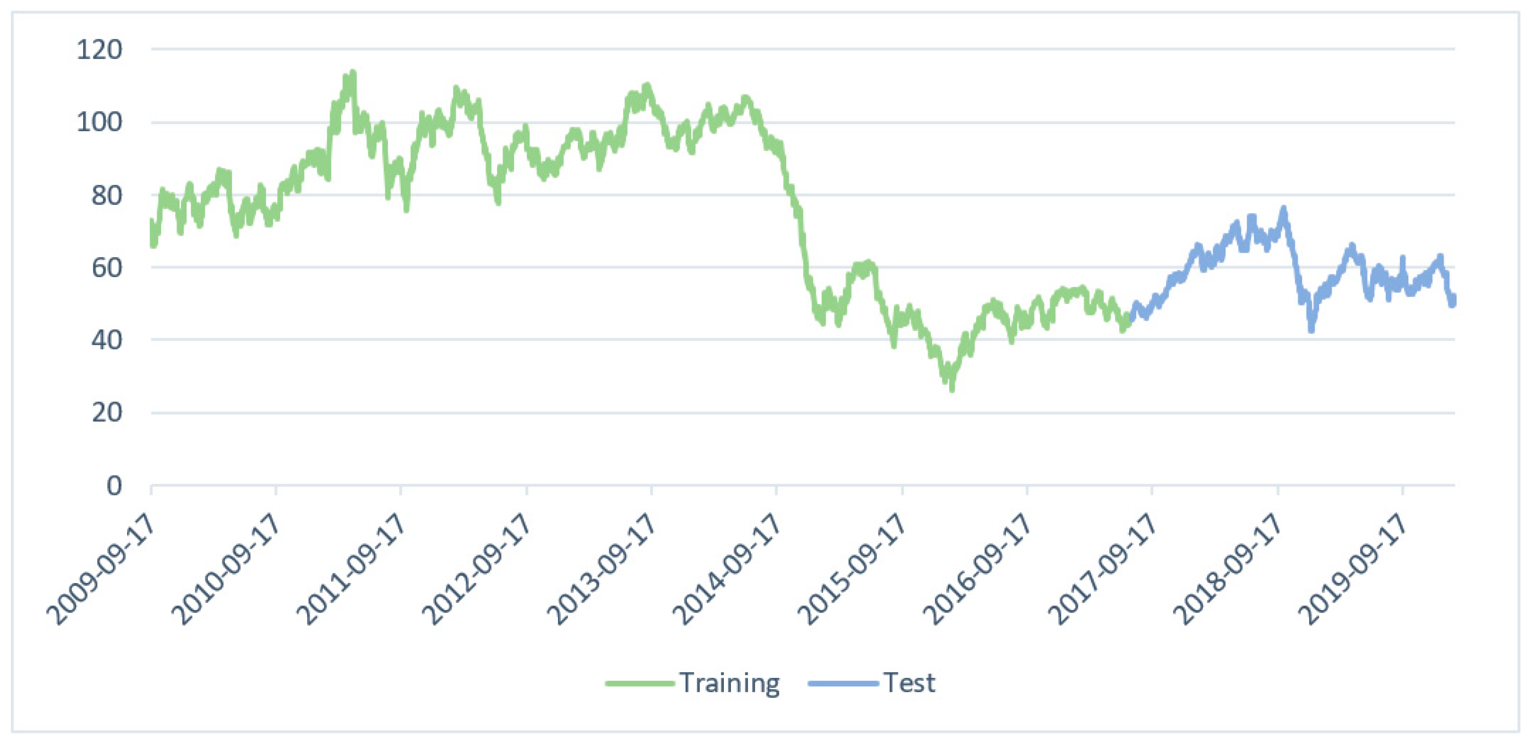
For the purpose of network operation, the data was divided into two sets—a training set and a test set. Figure 1 presents WTI futures prices quotations distinguished between a training set and a test set.

The set of observations was divided into a training set and a test set at a ratio of 75% to 25% respectively. A continuous set of observations, starting on 17th September 2009 and ending on 14th July 2017, was chosen as the training set. The observations constituting the test set cover the period from 17th July 2017 to 14th February 2020.

Table 1. Quantitative characteristics of training set and the test set.

	All	[>0]	[<0]	% All	% [>0]	% [<0]
Training set	1966	672	1294	75%	72%	76%
Test set	664	256	408	25%	28%	24%
Sum	2630	928	1702		35%	65%

presents quantitative characteristics of training data and test data. Column All contains the number of observations concerning the training and the test sets, as well as the number of all observations (Sum). Additionally, the Table 1 shows a division of observations of each set into cases that allowed obtaining a positive return from taking a long position in the call option ([>0]) and cases that generated a loss from taking a long position ([<0]). For each of the sets, the percentage share of the number of options generating profit in the number of options generating profit and coming from the whole set was also presented (% [>0]). Corresponding calculations were carried out for options that generated losses (% [<0]).

In the test sample, profit-generating observations had a higher percentage than it would appear from the percentage division of all observations into the training and the test sets. The proportion of loss-generating observations is also distorted in relation to the division ratio of the number of observations into the training and the test sets, but this deviation is insignificant. It is worth noting that almost twice as often (65% to 35%) the purchase of ATM options generates a loss rather than a profit. Generally speaking, an ATM call option usually has a delta, interpreted as the probability of exercising the option [56], at approximately 0.5. It should, however, be borne in mind that the option that will be exercised does not necessarily imply a profit to the buyer (cf. Equation (1)).

On the basis of the presented quantitative characteristics, it is possible to conclude that the probability of generating profit from taking a long position in the call option was higher for the test set.

Table 2. Value characteristics of training set and test set.

	All	[>0]	[<0]	% All	% [>0]	% [<0]
Training set	−277.18	1646.86	−1924.05	75%	81%	80%
Test set	−91.2	395.49	−486.69	25%	19%	20%
Sum	−368.39	2042.36	−2410.74

presents the value characteristics for each set. The first column of the table (All) should be understood as the amount of return on taking a long position in a call option on each subsequent day. The second and third columns are the sum of returns gathered from the observations generated only profit and loss.

The amount of the percentage return for each set is equal to the ratio of the division of observations into the training and the test sets (%All). On the basis of the percentage value, the shares of profits and losses from the purchase of options for the particular set in the total profit and loss figures, it can be concluded that the training set offers greater opportunities to achieve higher earnings as well as higher levels of loss. This issue is further detailed in

Table 3. Characteristics of training set and test set.

Interval (In USD)		Training Set		Test Set		Training Set		Test Set
for	to	Count	Value	Count	Value	%Count	%Value	%Count	%Value
−∞	−3	56	−204.6	9	−34.1	4.3%	10.6%	2.2%	7.0%
−3	−2	244	−585.9	42	−94.6	18.9%	30.5%	10.3%	19.4%
−2	−1	610	−904.9	182	−259.6	47.1%	47.0%	44.6%	53.3%
−1	0	384	−228.6	175	−98.4	29.7%	11.9%	42.9%	20.2%
Sum [>0]		1294	−1924.0	408	−486.7
0	1	211	102.0	110	48.4	31.4%	6.2%	43.0%	12.2%
1	2	142	210.4	65	94.0	21.1%	12.8%	25.4%	23.8%
2	3	122	306.0	48	117.3	18.2%	18.6%	18.8%	29.7%
3	∞	197	1028.4	33	135.8	29.3%	62.4%	12.9%	34.3%
Sum [<0]		672	1646.9	256	395.5
Sum all		1966	−277.2	664	−91.2

which contains both quantitative and value characteristics for each set. In addition, these characteristics were divided into value ranges representing the amount of return for the call option holder.

For each of the sets, the percentages of the above-mentioned characteristics were also presented in relation to the value of the number of all observations and the sum of returns from the purchase of an option, with a distinction between ranges of returns greater ([>0]) and smaller ([<0]) than zero. The final part presents quantitative and qualitative summaries for each of the sets and all observations together.

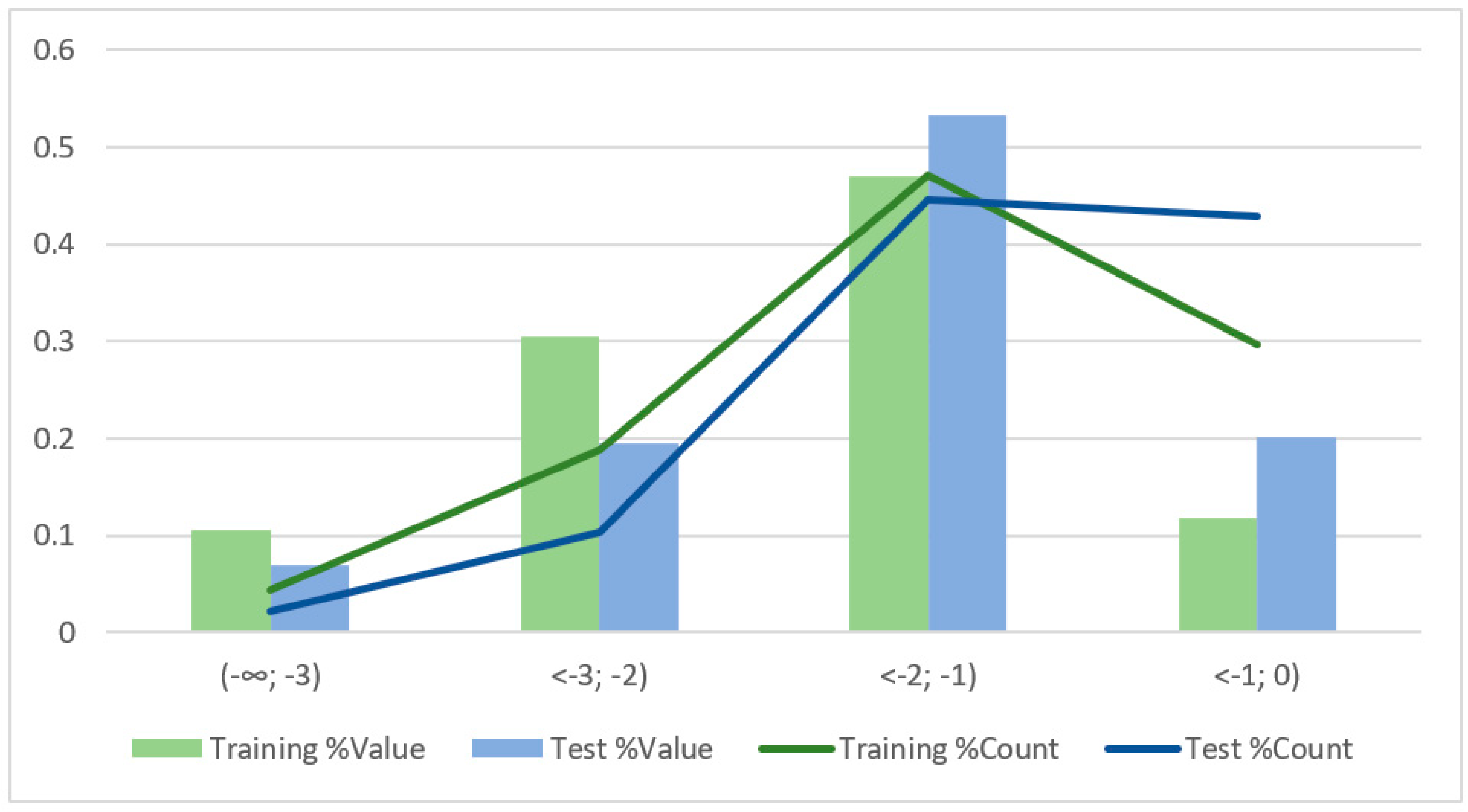
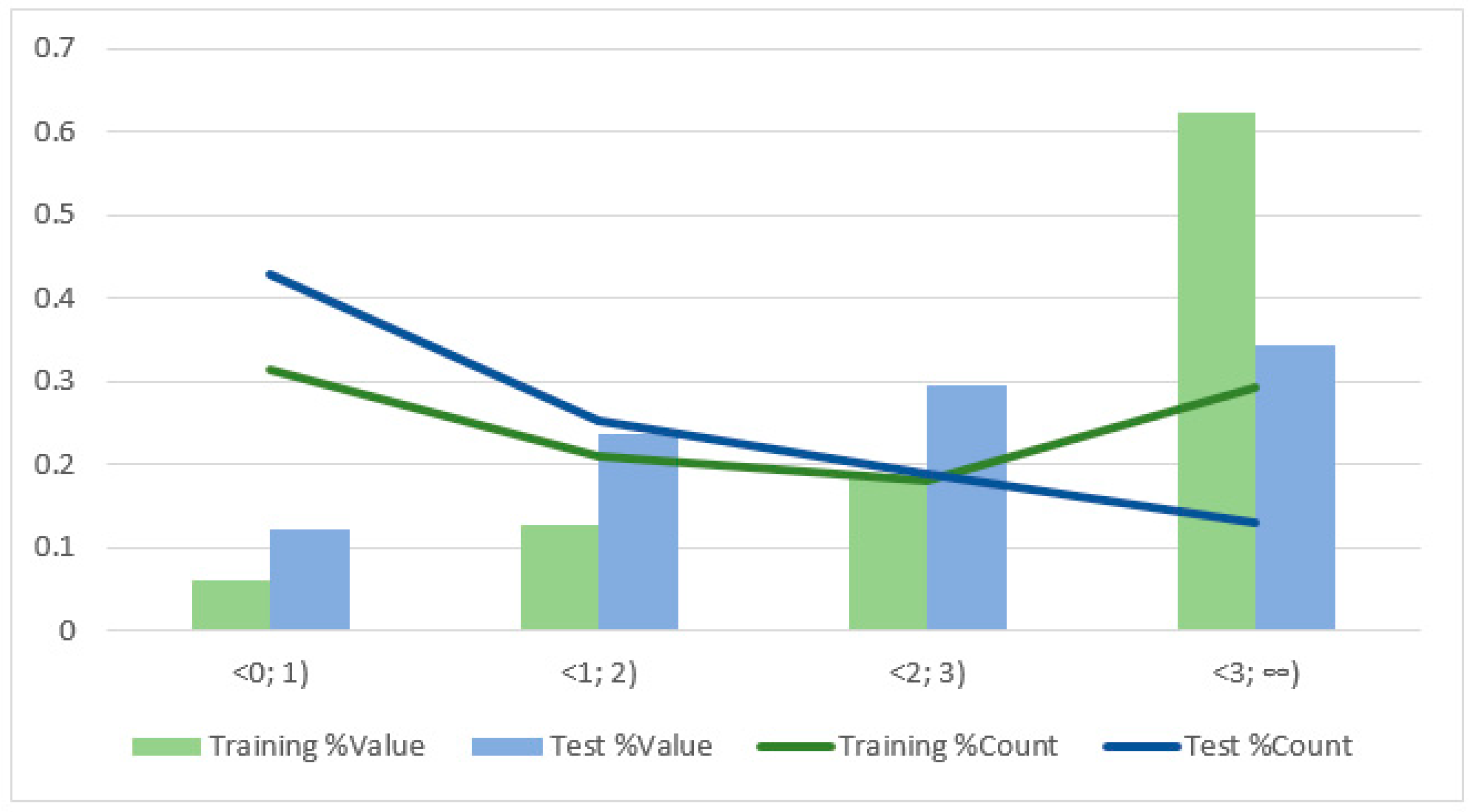
The data presented in Table 3 shows a much higher share of observations with high levels of loss and profit for the training set than for the test set. This means that there were many more observations with price increase in the training set (hence high profits in individual items) and the options were more expensive hedging instruments (which resulted in higher individual losses). In the case of losses, the percentage share of observations generating a loss of more than USD 2 is almost twice as high for the training set as for the test set. The situation is similar in the case of the amount of profit, i.e., more than twice as many observations of the training set generated profit above USD 3 as in the case of the test set. In the case of the test set, the share of observations generating small profits and small losses (up to USD 1) was significantly higher. The relations described are illustrated in Figure 2 and Figure 3.

As can be seen in Figure 3, an extremely strong imbalance occurs between the training and the test sets for profit over USD 3. For both, the training and the test sets, the value of the AR indicator (average return) is less than zero (

Table 4. Comparison of the values of indicators for the training set and the test set.

	AR	MP	ML
Training set	−277.18	1646.86	−1924.05
Test set	−91.20	395.49	−486.69

). Therefore, based on formula (2), the EP value for the particular network should be greater than zero, and not greater than the AR value.

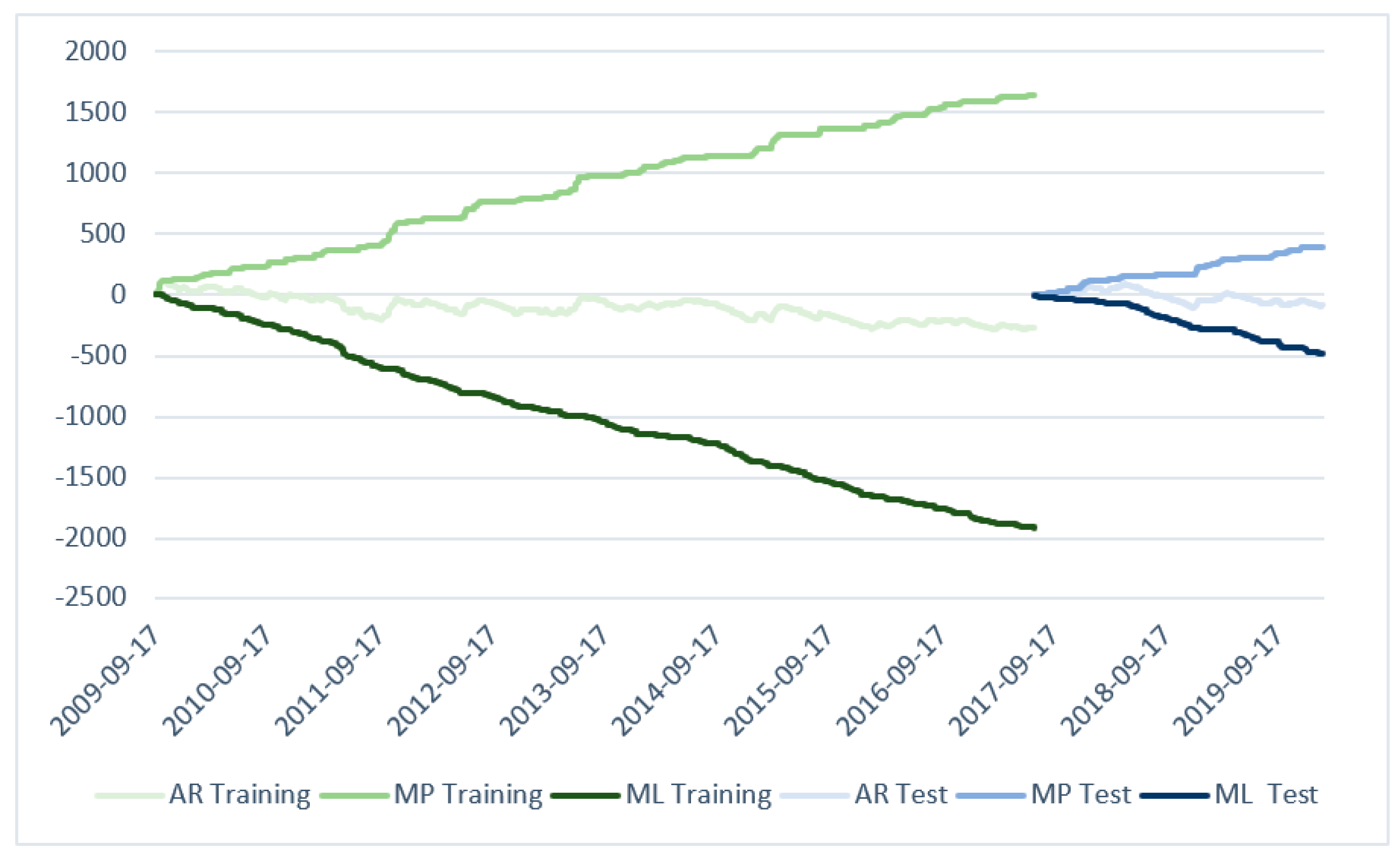
Figure 4 presents the values of the AR, MP and ML indicators on the timeline with a distinction between the training set and the test set.

The abovementioned parameters behave similarly for both sets. Greater deviations of the curves determined by the MP and ML indicators from the straight line ‘0′ occurring in the training set provide a visual confirmation of the conclusion that it is possible to achieve both greater loss and greater profit for the training set than for the test set. The next part of the study presents the results of SANN performance for the data sets described.

4. Results

The Statistica software (TIBCO Software Inc, Palo Alto, California, United States) was used to build the networks that were used to search for call option buy signals. The networks analyzed were classification networks and they were created using the automatic network selection tool built into the Statistica software. The networks created were MLP type networks with the number of neurons in the hidden layer between 5 and 30. The following indicators were used to assess the errors made by the network: sum of squares and joint entropy. The following functions were used as activation functions: linear, logistic, exponential, sinus and hyperbolic tangent (for the hidden and output layers) and softmax (for the output layer when joint entropy was used as the error evaluation function). For each type of activation function for the hidden layer neurons, 50,000 networks were trained. The best results (EP) for networks using a specific activation function (for the training set) are presented in

Table 5. Results (in USD/b) obtained in the SANN including the activation function used in the hidden layer.

Activation Function	BEST		AVG5		AVG10
	Training Set	Test Set	Training Set	Test Set	Training Set	Test Set
Linear	31.2	14.6	30.1	6.0	29.2	3.0
Sinus	215.0	50.1	197.7	40.1	182.9	38.0
Exponential	747.3	73.3	692.1	46.5	636.5	45.8
Hyperbolic tangent	1087.4	95.6	950.5	59.4	879.3	63.5
Logistic	1147.6	47.8	933.8	52.6	857.7	54.6

. Additionally, the average results of the best 5 and 10 solutions for the particular activation function used in the hidden layer are attached. This information has been added due to the fact that the results presented are best achieved by the networks for the training set, not the test one. Therefore, AVG5 and AVG10 results may be better than the BEST results but only for the test set.

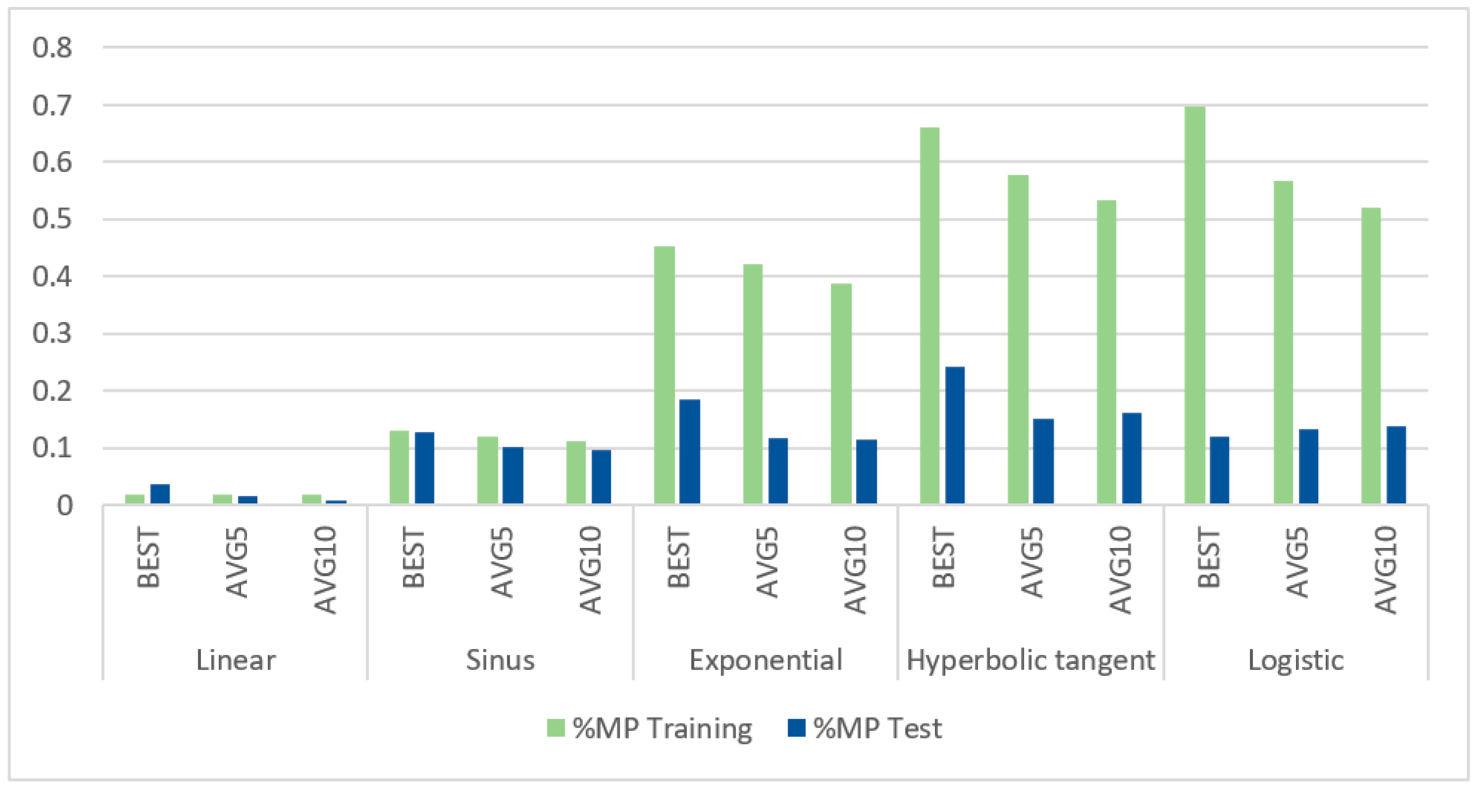
By far the worst results were obtained for the activation functions, linear and sinus (taking into account the training set). The best results, on the other hand, were obtained using the following functions: logistic and hyperbolic tangents. The results were also collated in Figure 5 using the %MP parameter which shows the percentage share of the network application result in the maximum profit that could have been obtained in the training set or on the test set (cf. Equation (11)).

The most distinctive result for the test set was obtained with the use of hyperbolic tangent as the activation function for the hidden layer neurons. Also noteworthy are the results obtained for the logistic activation function for which the average values calculated for the test set are higher than those for the BEST solution.

Based on the presented results, it was decided to carry out additional tests for three hidden layer activation functions, allowing to obtain the best solutions. Two output layer activation functions (logistic, softmax) were selected, which enabled to obtain the best results for the selected hidden layer activation functions (detailed results for the best 10 solutions for each particular activation function can be found in Appendix A (

Table A1. Best SANN’s results.

Num.	Training Set	Test Set	SANN’s Name	Training Algorithm	Error Function	Hidden Layer	Output Layer	Test Number
1	1147.6	47.8	MLP 53-16-2	BFGS 76	Entropy	Logistic	Softmax	T1
2	948.8	44.1	MLP 53-9-2	BFGS 52	SOS	Logistic	Logistic	T1
3	929.6	60.1	MLP 53-7-2	BFGS 77	SOS	Logistic	Logistic	T1
4	838.7	77.4	MLP 53-8-2	BFGS 55	Entropy	Logistic	Softmax	T1
5	804.4	33.8	MLP 53-7-2	BFGS 53	Entropy	Logistic	Softmax	T1
6	801.3	59.0	MLP 53-12-2	BFGS 53	Entropy	Logistic	Softmax	T1
7	800.1	45.8	MLP 53-6-2	BFGS 70	SOS	Logistic	Logistic	T1
8	778.1	46.2	MLP 53-9-2	BFGS 53	SOS	Logistic	Logistic	T1
9	768.5	59.6	MLP 53-5-2	BFGS 67	SOS	Logistic	Logistic	T1
10	759.7	72.1	MLP 53-6-2	BFGS 101	SOS	Logistic	Logistic	T1
11	31.2	14.6	MLP 53-13-2	BFGS 28	Entropy	Linear	Softmax	T1
12	30.7	2.1	MLP 53-28-2	BFGS 25	Entropy	Linear	Softmax	T1
13	29.8	15.2	MLP 53-9-2	BFGS 25	SOS	Linear	Exponential	T1
14	29.4	0.1	MLP 53-19-2	BFGS 26	Entropy	Linear	Softmax	T1
15	29.2	−2.2	MLP 53-6-2	BFGS 30	Entropy	Linear	Softmax	T1
16	28.4	0.5	MLP 53-17-2	BFGS 25	Entropy	Linear	Softmax	T1
17	28.4	0.5	MLP 53-6-2	BFGS 29	Entropy	Linear	Softmax	T1
18	28.3	−0.9	MLP 53-19-2	BFGS 20	Entropy	Linear	Softmax	T1
19	28.2	0.1	MLP 53-21-2	BFGS 18	Entropy	Linear	Softmax	T1
20	28.0	0.1	MLP 53-5-2	BFGS 24	Entropy	Linear	Softmax	T1
21	215.0	50.1	MLP 53-5-2	BFGS 30	SOS	Sinus	Hyperbolic tangent	T1
22	209.2	24.2	MLP 53-6-2	BFGS 62	Entropy	Sinus	Softmax	T1
23	201.3	43.7	MLP 53-5-2	BFGS 24	SOS	Sinus	Hyperbolic tangent	T1
24	188.6	46.0	MLP 53-6-2	BFGS 42	SOS	Sinus	Logistic	T1
25	174.2	36.5	MLP 53-8-2	BFGS 28	SOS	Sinus	Hyperbolic tangent	T1
26	173.9	38.8	MLP 53-7-2	BFGS 27	Entropy	Sinus	Softmax	T1
27	172.2	44.4	MLP 53-28-2	BFGS 22	Entropy	Sinus	Softmax	T1
28	168.8	44.1	MLP 53-8-2	BFGS 27	SOS	Sinus	Exponential	T1
29	165.4	39.8	MLP 53-7-2	BFGS 49	SOS	Sinus	Exponential	T1
30	160.8	12.5	MLP 53-20-2	BFGS 38	Entropy	Sinus	Softmax	T1
31	1087.4	95.6	MLP 53-17-2	BFGS 88	Entropy	Hyperbolic tangent	Softmax	T1
32	1008.7	52.9	MLP 53-12-2	BFGS 83	Entropy	Hyperbolic tangent	Softmax	T1
33	928.5	49.9	MLP 53-26-2	BFGS 69	Entropy	Hyperbolic tangent	Softmax	T1
34	874.3	56.1	MLP 53-22-2	BFGS 60	Entropy	Hyperbolic tangent	Softmax	T1
35	853.7	42.3	MLP 53-15-2	BFGS 57	Entropy	Hyperbolic tangent	Softmax	T1
36	844.5	64.7	MLP 53-10-2	BFGS 68	Entropy	Hyperbolic tangent	Softmax	T1
37	824.6	53.1	MLP 53-23-2	BFGS 51	SOS	Hyperbolic tangent	Logistic	T1
38	813.3	86.6	MLP 53-6-2	BFGS 128	Entropy	Hyperbolic tangent	Softmax	T1
39	779.9	40.9	MLP 53-22-2	BFGS 53	Entropy	Hyperbolic tangent	Softmax	T1
40	777.8	92.5	MLP 53-14-2	BFGS 56	Entropy	Hyperbolic tangent	Softmax	T1
41	747.3	73.3	MLP 53-6-2	BFGS 77	Entropy	Exponential	Softmax	T1
42	710.8	47.5	MLP 53-25-2	BFGS 121	Entropy	Exponential	Softmax	T1
43	709.0	22.2	MLP 53-7-2	BFGS 65	Entropy	Exponential	Softmax	T1
44	646.8	58.6	MLP 53-6-2	BFGS 59	Entropy	Exponential	Softmax	T1
45	646.5	30.8	MLP 53-25-2	BFGS 105	Entropy	Exponential	Softmax	T1
46	622.2	66.9	MLP 53-26-2	BFGS 94	Entropy	Exponential	Softmax	T1
47	599.2	49.3	MLP 53-19-2	BFGS 77	Entropy	Exponential	Softmax	T1
48	568.7	20.4	MLP 53-19-2	BFGS 84	Entropy	Exponential	Softmax	T1
49	558.6	45.2	MLP 53-26-2	BFGS 89	Entropy	Exponential	Softmax	T1
50	555.6	43.8	MLP 53-21-2	BFGS 61	Entropy	Exponential	Softmax	T1
1	1085.0	69.6	MLP 53-11-2	BFGS 131	SOS	Logistic	Logistic	T2
2	1016.9	67.7	MLP 53-13-2	BFGS 103	SOS	Logistic	Logistic	T2
3	951.1	45.2	MLP 53-11-2	BFGS 91	SOS	Logistic	Logistic	T2
4	946.4	61.9	MLP 53-10-2	BFGS 96	SOS	Logistic	Logistic	T2
5	943.1	61.1	MLP 53-9-2	BFGS 108	SOS	Logistic	Logistic	T2
6	939.8	64.0	MLP 53-10-2	BFGS 78	SOS	Logistic	Logistic	T2
7	921.7	59.5	MLP 53-13-2	BFGS 72	SOS	Logistic	Logistic	T2
8	911.1	70.4	MLP 53-18-2	BFGS 61	SOS	Logistic	Logistic	T2
9	904.6	69.1	MLP 53-7-2	BFGS 146	SOS	Logistic	Logistic	T2
10	895.5	70.2	MLP 53-8-2	BFGS 160	SOS	Logistic	Logistic	T2
11	1175.2	67.8	MLP 53-14-2	BFGS 90	Entropy	Logistic	Softmax	T2
12	1146.5	64.9	MLP 53-21-2	BFGS 67	Entropy	Logistic	Softmax	T2
13	1001.0	50.7	MLP 53-11-2	BFGS 66	Entropy	Logistic	Softmax	T2
14	981.6	32.6	MLP 53-14-2	BFGS 89	Entropy	Logistic	Softmax	T2
15	977.8	68.2	MLP 53-9-2	BFGS 67	Entropy	Logistic	Softmax	T2
16	921.5	69.3	MLP 53-13-2	BFGS 94	Entropy	Logistic	Softmax	T2
17	898.6	67.4	MLP 53-12-2	BFGS 60	Entropy	Logistic	Softmax	T2
18	875.6	42.2	MLP 53-26-2	BFGS 52	Entropy	Logistic	Softmax	T2
19	861.9	19.0	MLP 53-13-2	BFGS 88	Entropy	Logistic	Softmax	T2
20	857.6	68.8	MLP 53-7-2	BFGS 63	Entropy	Logistic	Softmax	T2
21	1135.7	63.0	MLP 53-24-2	BFGS 106	SOS	Hyperbolic tangent	Logistic	T2
22	1032.9	64.5	MLP 53-11-2	BFGS 61	SOS	Hyperbolic tangent	Logistic	T2
23	1026.2	26.5	MLP 53-28-2	BFGS 59	SOS	Hyperbolic tangent	Logistic	T2
24	827.2	47.1	MLP 53-8-2	BFGS 75	SOS	Hyperbolic tangent	Logistic	T2
25	825.9	46.0	MLP 53-16-2	BFGS 57	SOS	Hyperbolic tangent	Logistic	T2
26	812.0	45.8	MLP 53-8-2	BFGS 42	SOS	Hyperbolic tangent	Logistic	T2
27	797.1	37.7	MLP 53-5-2	BFGS 42	SOS	Hyperbolic tangent	Logistic	T2
28	782.8	30.8	MLP 53-8-2	BFGS 66	SOS	Hyperbolic tangent	Logistic	T2
29	766.0	29.1	MLP 53-11-2	BFGS 42	SOS	Hyperbolic tangent	Logistic	T2
30	761.4	66.2	MLP 53-7-2	BFGS 47	SOS	Hyperbolic tangent	Logistic	T2
31	1045.7	39.8	MLP 53-13-2	BFGS 63	Entropy	Hyperbolic tangent	Softmax	T2
32	1011.8	49.0	MLP 53-26-2	BFGS 102	Entropy	Hyperbolic tangent	Softmax	T2
33	1000.8	89.8	MLP 53-13-2	BFGS 64	Entropy	Hyperbolic tangent	Softmax	T2
34	978.1	57.0	MLP 53-24-2	BFGS 117	Entropy	Hyperbolic tangent	Softmax	T2
35	949.5	71.5	MLP 53-17-2	BFGS 105	Entropy	Hyperbolic tangent	Softmax	T2
36	941.1	75.0	MLP 53-20-2	BFGS 60	Entropy	Hyperbolic tangent	Softmax	T2
37	938.3	66.2	MLP 53-27-2	BFGS 55	Entropy	Hyperbolic tangent	Softmax	T2
38	930.0	43.4	MLP 53-14-2	BFGS 83	Entropy	Hyperbolic tangent	Softmax	T2
39	918.9	49.0	MLP 53-18-2	BFGS 82	Entropy	Hyperbolic tangent	Softmax	T2
40	913.0	86.3	MLP 53-14-2	BFGS 110	Entropy	Hyperbolic tangent	Softmax	T2
41	719.7	70.5	MLP 53-6-2	BFGS 186	SOS	Exponential	Logistic	T2
42	656.8	43.3	MLP 53-6-2	BFGS 81	SOS	Exponential	Logistic	T2
43	647.5	52.9	MLP 53-6-2	BFGS 83	SOS	Exponential	Logistic	T2
44	627.2	106.5	MLP 53-6-2	BFGS 191	SOS	Exponential	Logistic	T2
45	623.5	50.3	MLP 53-8-2	BFGS 78	SOS	Exponential	Logistic	T2
46	613.8	46.1	MLP 53-6-2	BFGS 123	SOS	Exponential	Logistic	T2
47	607.4	69.9	MLP 53-8-2	BFGS 59	SOS	Exponential	Logistic	T2
48	606.6	59.6	MLP 53-5-2	BFGS 90	SOS	Exponential	Logistic	T2
49	595.8	59.7	MLP 53-9-2	BFGS 54	SOS	Exponential	Logistic	T2
50	595.0	31.4	MLP 53-8-2	BFGS 73	SOS	Exponential	Logistic	T2
51	847.0	45.7	MLP 53-11-2	BFGS 89	Entropy	Exponential	Softmax	T2
52	821.9	48.3	MLP 53-19-2	BFGS 119	Entropy	Exponential	Softmax	T2
53	820.1	31.2	MLP 53-9-2	BFGS 90	Entropy	Exponential	Softmax	T2
54	792.1	53.0	MLP 53-12-2	BFGS 95	Entropy	Exponential	Softmax	T2
55	787.2	30.3	MLP 53-9-2	BFGS 106	Entropy	Exponential	Softmax	T2
56	773.4	45.6	MLP 53-19-2	BFGS 104	Entropy	Exponential	Softmax	T2
57	759.2	29.0	MLP 53-14-2	BFGS 101	Entropy	Exponential	Softmax	T2
58	752.1	49.5	MLP 53-9-2	BFGS 77	Entropy	Exponential	Softmax	T2
59	723.7	32.6	MLP 53-7-2	BFGS 71	Entropy	Exponential	Softmax	T2
60	723.5	41.4	MLP 53-20-2	BFGS 80	Entropy	Exponential	Softmax	T2

) and are marked as T1 set). For each combination of selected activation functions in the hidden layer and the output layer, 100,000 networks were trained. The obtained results (marked as T2 in Table A1) are shown in

Table 6. Results (in USD/b) obtained in the SANN with a division into activation functions used in the hidden layer and in the output layer.

Activation Function		BEST		AVG5		AVG10
Hidden Layer	Output Layer	Training Set	Test Set	Training Set	Test Set	Training Set	Test Set
Logistic	Logistic	1085.0	69.6	988.5	61.1	951.5	63.9
Logistic	Softmax	1175.2	67.8	1056.4	56.8	969.7	55.1
Hyperbolic tangent	Logistic	1135.7	63.0	969.6	49.4	876.7	45.7
Hyperbolic tangent	Softmax	1045.7	39.8	997.2	61.4	962.7	62.7
Exponential	Logistic	719.7	70.5	654.9	64.7	629.3	59.0
Exponential	Softmax	847.0	45.7	813.7	41.7	780.0	40.7

.

For each of the analyzed activation functions of the hidden layer in the T2 set, an improvement of the best result for the test set was obtained as compared with the T1 set. The values of the %MP parameter obtained for the T2 set are presented in Figure 6.

Repeated calculations confirmed that the worst results for the training set were obtained using the exponential activation function in the hidden layer. At the same time, the exponential activation function (using the logistic activation function for the output layer) enabled to obtain the best (of the 6 cases considered in the T2 set) BEST result. Also noteworthy are the results of hyperbolic tangents for the softmax function, where an upward trend is visible for the consecutive values considered. This may indicate a low value of the BEST result for the test set as compared with the results of the next networks (with similar parameters).

Table 7. Top 10 SANN results (in USD/b).

Num.	Activation Function		Result	Training Set	Test Set	% MP Training Set	% MP Test Set
	Hidden Layer	Output Layer
1	Logistic	Softmax	BEST	1175.2	67.8	71.4%	17.1%
2	Logistic	Softmax	BEST	1147.6	47.8	69.7%	12.1%
3	Logistic	Softmax	BEST	1146.5	64.9	69.6%	16.4%
4	Hyperbolic tangent	Logistic	BEST	1135.7	63.0	69.0%	15.9%
5	Hyperbolic tangent	Softmax	BEST	1087.4	95.6	66.0%	24.2%
6	Logistic	Logistic	BEST	1085.0	69.6	65.9%	17.6%
7	Logistic	Softmax	AVG5	1056.4	56.8	64.1%	14.4%
8	Hyperbolic tangent	Softmax	BEST	1045.7	39.8	63.5%	10.1%
9	Hyperbolic tangent	Logistic	BEST	1032.9	64.5	62.7%	16.3%
10	Hyperbolic tangent	Logistic	BEST	1026.2	26.5	62.3%	6.7%
AVG				1093.9	59.6	66.4%	15.1%

presents a summary containing the results (for the training set) obtained by the 10 best networks (from T1 and T2 sets). It is noteworthy that the average of the 5 best results for the logistic activation function is presented with an error assessment based on the entropy coefficient.

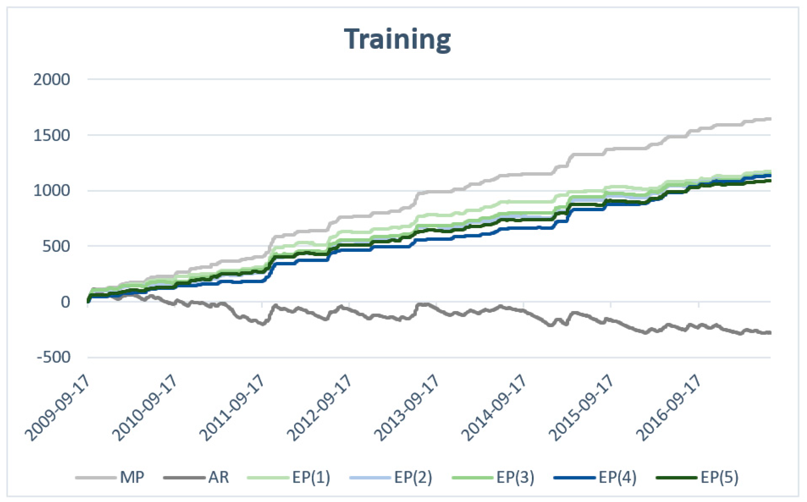
For the five networks that yielded the best results (Table 7, numbers 1–5), the graphs were made to show the change in time of the values of the MP, AR and EP indicators. Figure 7 presents the values of MP, AR and EP for the training set, while Figure 8 presents the values for the test set. The value in brackets by the EP coefficient refers to the network number in Table 7.

The difference on the last day included in the training set between the highest and the lowest values of the %MP indicator for the five networks under consideration is 5.4%. It is worth noting that this value (Max (%MP)-Min (%MP)) was not less than 20% for nearly 2/3 of the number of training set observations. This difference is particularly visible in the central part of the chart, where the curves clearly diverge to ‘get closer’ towards the end of the training set. For all the networks, there is a clear tendency in which the value of the EP indicator ‘follows’ the MP indicator.

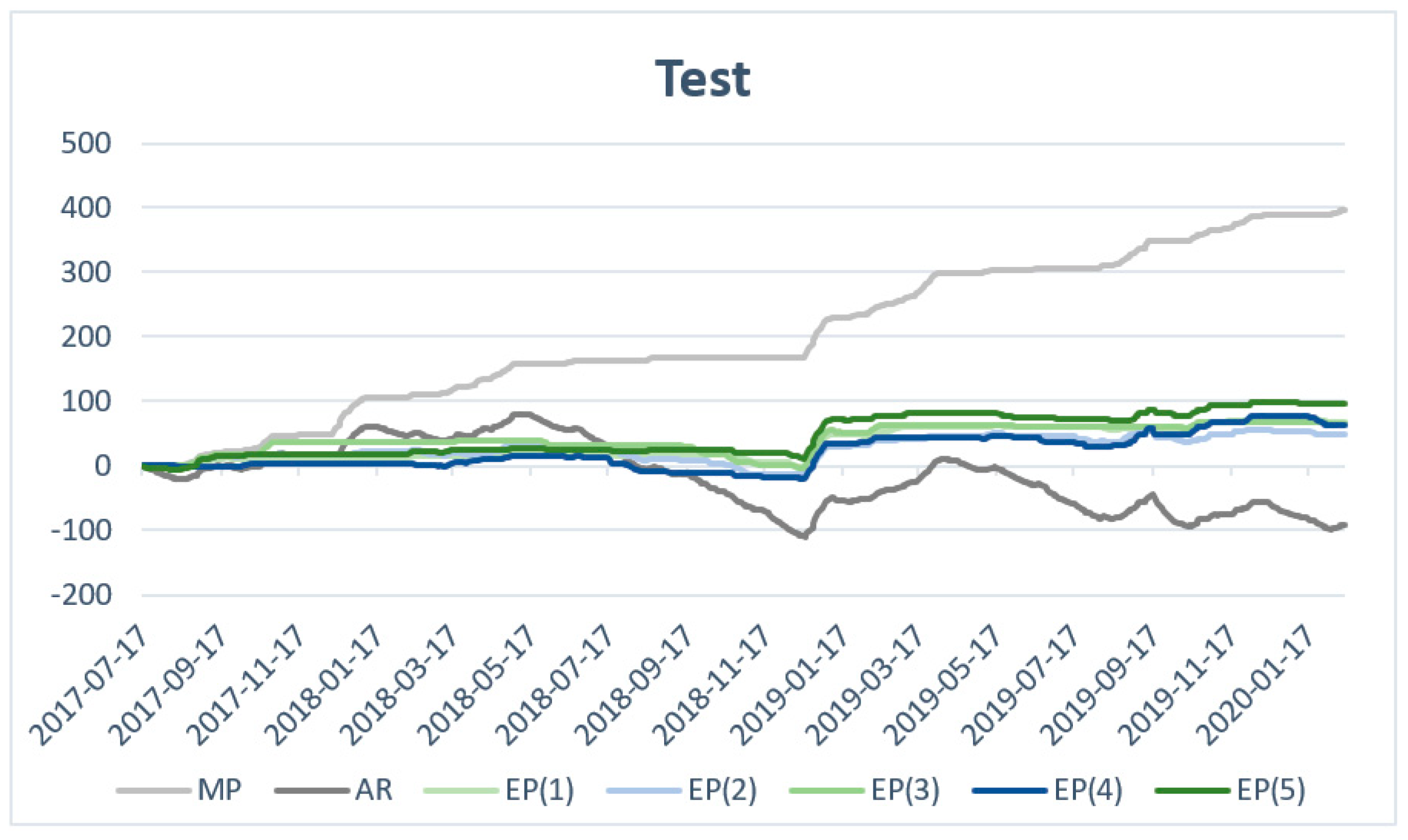
For the test set, the results obtained by the networks (EP) are significantly worse than for the training set. Figure 8 also shows that the relation between the MP and EP values for the test set is much weaker (less favorable from the perspective of a call option buyer) than for the training set. It is also worth noting that for the data set corresponding to the first half of 2018, the value of the AR indicator exceeds the values of the EP indicators. Furthermore, only a weak reaction of the EP indicators to the changes in the AR indicator can be observed.

For the test set, the difference between the highest and the lowest values of %MP is almost twice as high as for the training set and amounts to 12.1%. This value also means that the best solution out of the five considered networks (%MP (5) = 24.2%) is twice as good as the worst solution (%MP (2) = 12.1%).

Table 8. Results obtained by the top 5 SANNs in the training set.

			(1)	(2)	(3)	(4)	(5)
Count	Training set	Correct	523	507	511	461	514
		Incorrect	112	144	138	28	137
		Total	635	651	649	489	651
	Test set	Correct	69	108	62	89	86
		Incorrect	52	88	54	71	50
		Total	121	196	116	160	136
Value	Training set	Correct	1319.4	1330.0	1323.3	1183.3	1245.9
		Incorrect	−144.2	−182.3	−176.8	−47.6	−158.5
		Total	1175.2	1147.6	1146.5	1135.7	1087.4
	Test set	Correct	119.6	156.6	123.0	150.6	148.4
		Incorrect	−51.8	−108.8	−58.0	−87.6	−52.8
		Total	67.8	47.8	64.9	63.0	95.6

presents detailed quantitative and qualitative information on the five networks that allow to obtain the best result in the training set.

Only one of the discussed networks generated fewer than 500 buy signals for the training set, i.e., network number 4. This network was also distinguished by a very low value of incorrectly generated buy signals for the training set, which also resulted in a small loss due to buying options based on incorrect signals. The remaining networks generated a similar number of buy signals for the training set, in the range between 635 and 651. For three networks, the return on buying a hedge based on correctly generated buy signals for the training set exceeded the value of USD 1300. In the case of the test set, the results obtained by the networks based on correctly generated buy signals can be divided into two classes:

(1)

Networks allowing revenue of approx. USD 120

(2)

Networks generating revenue of approx. USD 150

The network that achieved a significantly higher %MP rate as compared with the other ones is the network (5). It is worth noting that this network is not distinguished by either the number of correctly or erroneously generated buy signals for the test set or the profit or loss achieved by these signals.

When analyzing the data included in Table 8, two strategies of generating buy signals can be distinguished. The first can be described as ‘many bad, many (more) good’ (MBMG). It consists in frequent generation of buy signals, a large portion of which may turn out to be incorrect; however, a much larger proportion of the signals (allowing to obtain a positive value of the EP indicator) is generated correctly. The second strategy (the use of which can only be observed in the case of the network (4) for the training set) can be characterized as: ‘few good, fewer bad’ (FGFB). It consists in limiting the number of generated buy signals (even at the expense of a smaller number of profit-generating signals), while strongly limiting the number of loss-generating signals.

The undoubted advantage of the MBMG strategy is that it is more likely (based on the number of long positions taken in call options) to hedge against unexpected but significant increases in WTI oil prices. On the other hand, the cost of frozen capital for the FGFB strategy is much lower. Also, the costs associated with the purchase of options are lower (the total of option premiums paid).

5. Conclusions and Future Research Directions

This paper thoroughly examines the ability of artificial neural networks as a tool to support the decision-making process concerning hedging WTI oil prices with the use of option contracts. We analyze the selection of the activation function both in the hidden layer and in the output layer. Due to the limitations of Statistica, there was only one hidden layer in the given networks. The parameter of the number of neurons in the hidden layer was limited by the range from 5 to 30. Using the Statistica automatic network selection tool, this size was modified (see Appendix A, Table A1, column “SANN’s Name”) to obtain the highest value of the quality of the network matching. Research outcomes revealed that the networks with the best results used the Logistic activation function in the hidden layer and the Softmax activation function in the output layer for the number of neurons between 5 and 25.

As the research has shown, the situations where an option was not exercised or could have been exercised at a loss (the option premium was greater than the difference between the oil price on the expiry date of the option and the option strike price) were much more common in the analyzed period. As a result, the value of the AR (average return) indicator for both the training and the test sets was less than zero. The given networks (SANNs) made it possible to generate buy signals for which the sum of results obtained from long positions in call options was positive not only in the training set but also in the test set. What is more, the values of the %MP indicator for the best networks in the training set were between 12–24% in the test set, which should be considered a promising result from the perspective of further research. For future work, the following potential research directions were distinguished:

• Possible use of neural networks to search for buy or sell signals of other types of options (such as put options and American options);
• Possible use of a network to improve the performance of option strategies that require the acquiring and issuing (buying and selling) options that differ in terms of parameters such as strike price and exercise dates;
• Possible use of the proposed model to support the process of making decisions whether or not to purchase a hedge in other raw material markets;
• An attempt to improve the results obtained by networks for the test set.

References

- Tsai, C. How do U.S. stock returns respond differently to oil price shocks pre-crisis, within the financial crisis, and post-crisis? Energy Econ. 2015, 50, 47–62. [Google Scholar] [CrossRef]
- BP Statistical Review of World Energy. Available online: https://www.bp.com/en/global/corporate/energy-economics/statistical-review-of-world-energy.html (accessed on 20 November 2019).
- Hamilton, J.D. Oil and the macroeconomy since World War II. J. Pol. Econ. 1983, 92, 228–248. [Google Scholar] [CrossRef]
- Hamilton, J.D. What is an oil shock? J. Econ. 2003, 113, 363–398. [Google Scholar] [CrossRef]
- Kilian, L. Exogenous oil supply shocks: How big are they and how much do they matter for the US economy? Rev. Econ. Stat. 2008, 90, 216–240. [Google Scholar] [CrossRef]
- Lee, C.C.; Lee, C.C.; Ning, S.L. Dynamic relationship of oil price shocks and country risks. Energy Econ. 2017, 66, 571–581. [Google Scholar] [CrossRef]
- Arouri, M.; Jouini, J.; Nguyen, K.D. On the impacts of oil price fluctuations on European equity markets: Volatility spillover and hedging effectiveness. Energy Econ. 2012, 34, 611–617. [Google Scholar] [CrossRef]
- Cuando, J.; de Garcia, F.P. Oil price shocks and stock market returns: Evidence for some European countries. Energy Econ. 2014, 42, 365–377. [Google Scholar] [CrossRef]
- Bagirov, M.; Mateus, C. Oil prices, stock markets and firm performance: Evidence from Europe. Int. Rev. Econ. Financ. 2019, 61, 270–288. [Google Scholar] [CrossRef]
- Kilian, L. Not all oil shocks are alike: Disentangling demand and supply shocks in the crude oil market. Am. Econ. Rev. 2009, 99, 1053–1069. [Google Scholar] [CrossRef] [Green Version]
- Kilian, L.; Park, C. The impact of oil price shocks on the US stock market. Int. Econ. Rev. 2009, 50, 1267–1287. [Google Scholar] [CrossRef]
- Kang, W.; Ratti, R.A.; Vespignani, J. The impact of oil price shocks on the U.S. stock market: A note on the roles of US and non-U.S. oil production. Econ. Lett. 2016, 145, 176–181. [Google Scholar] [CrossRef] [Green Version]
- Lambertides, N.; Savva, C.S.; Tsouknidis, D.A. The effects of oil price shocks on U.S. stock order flow imbalances and stock returns. J. Int. Money Financ. 2017, 74, 137–146. [Google Scholar] [CrossRef]
- Broadstock, D.C.; Filis, G. Oil price shocks and stock market returns: New evidence from the United States and China. J. Int. Financ. Mark. Inst. Money 2014, 33, 417–433. [Google Scholar] [CrossRef] [Green Version]
- Li, P.; Zhang, Z.; Yang, T.; Zeng, Q. The relationship among China’s fuel oil spot, futures and stock markets. Financ. Res. Lett. 2018, 24, 151–162. [Google Scholar]
- Li, X.; Wei, Y. The dependence and risk spillover between crude oil market and China stock market: New evidence from a variational mode decomposition-based copula method. Energy Econ. 2018, 74, 565–581. [Google Scholar] [CrossRef]
- Wei, Y.; Qin, S.; Li, X.; Zhu, S.; Wei, G. Oil price fluctuation, stock market and macroeconomic fundamentals: Evidence from China before and after the financial crisis. Financ. Res. Lett. 2019, 30, 23–29. [Google Scholar] [CrossRef]
- Yu, L.; Wang, Z.; Tang, L. A decomposition-ensemble model with data-characteristic-driven reconstruction for crude oil price forecasting. Appl. Energy 2015, 156, 251–267. [Google Scholar] [CrossRef]
- An, J.; Mikhaylov, A.; Moiseev, N. Oil price predictors: Machine learning approach. Int. J. Energy Econ. Policy 2019, 9, 1–6. [Google Scholar] [CrossRef] [Green Version]
- Aleksendrić, D.; Carlone, P. Soft Computing in the Design and Manufacturing of Composite Materials. Applications to Brake Friction and Thermoset Matrix Composites; Woodhead Publishing: London, UK, 2015; pp. 39–60. [Google Scholar]
- Sadorsky, P. Modeling and forecasting petroleum futures volatility. Energy Econ. 2006, 28, 467–488. [Google Scholar] [CrossRef]
- Cheong, C.W. Modeling and forecasting crude oil markets using ARCH-type models. Energy Policy 2009, 37, 2346–2355. [Google Scholar] [CrossRef]
- Kang, S.H.; Kang, S.; Yoon, S. Forecasting volatility of crude oil markets. Energy Econ. 2009, 31, 119–125. [Google Scholar] [CrossRef]
- Mohammadi, H.; Su, L. International evidence on crude oil price dynamics: Applications of ARIMA-GARCH models. Energy Econ. 2010, 32, 1001–1008. [Google Scholar] [CrossRef]
- Wei, Y.; Wang, Y.; Huang, D. Forecasting crude oil market volatility: Further evidence using GARCH-class models. Energy Econ. 2010, 32, 1477–1484. [Google Scholar] [CrossRef]
- Kang, S.H.; Yoon, S. Modeling and forecasting the volatility of petroleum futures prices. Energy Econ. 2012, 36, 354–362. [Google Scholar] [CrossRef]
- Zhao, C.L.; Wang, B. Forecasting Crude Oil Price with an Autoregressive Integrated Moving Average (ARIMA) Model. In Fuzzy Information & Engineering and Operations Research & Management; Cao, B., Nasseri, H., Eds.; Springer: Berlin/Heidelberg, Germany, 2014; Volume 211, pp. 275–286. [Google Scholar]
- Aamir, M.; Shabri, A. Modelling and Forecasting Monthly Crude Oil Price of Pakistan: A Comparative Study of ARIMA, GARCH and ARIMA Kalman Mode. In Proceedings of the Advances in Industrial and Applied Mathematics, Johor Bahru, Malaysia, 24–26 November 2015; Salleh, S., Aris, N., Bahar, A., Zainuddin, Z.M., Maan, N., Lee, M.H., Ahmad, T., Yusof, Y.M., Eds.; AIP Publishing LLC: Melville, NY, USA, 2016; Volume 1750. [Google Scholar]
- Nademi, A.; Nademi, Y. Forecasting crude oil prices by a semiparametric Markov switching model: OPEC, WTI, and Brent cases. Energy Econ. 2018, 74, 757–766. [Google Scholar] [CrossRef]
- Lin, H.; Su, Q. Crude Oil Prices Forecasting: An Approach of Using CEEMDAN-Based Multi-Layer Gated Recurrent Unit Networks. Energies 2020, 13, 1543. [Google Scholar] [CrossRef] [Green Version]
- Li, J.; Zhu, S.; Wu, O. Monthly crude oil spot price forecasting using variational mode decomposition. Energy Econ. 2019, 83, 240–253. [Google Scholar] [CrossRef]
- Azadeh, A.; Moghaddam, M.; Khakzad, M.; Ebrahimipour, V. A flexible neural network-fuzzy mathematical programming algorithm for improvement of oil price estimation and forecasting. Comput. Ind. Eng. 2012, 62, 421–430. [Google Scholar] [CrossRef]
- Chiroma, H.; Abdulkareem, S.; Herawan, T. Evolutionary neural network model for West Texas Intermediate crude oil price prediction. Appl. Energy 2015, 142, 266–273. [Google Scholar] [CrossRef]
- Wang, J.; Wang, J. Forecasting energy market indices with recurrent neural networks: Case study of crude oil price fluctuations. Energy 2016, 102, 365–374. [Google Scholar] [CrossRef]
- Mohamed, M.M.; El-Masry, A.A. Oil price forecasting using gene expression programming and artificial neural networks. Econ. Model. 2016, 54, 40–53. [Google Scholar]
- Huang, L.; Wang, J. Global crude oil price prediction and synchronization based accuracy evaluation using random wavelet neural network. Energy 2018, 151, 875–888. [Google Scholar] [CrossRef]
- Safari, A.; Davallou, M. Oil price forecasting using a hybrid model. Energy 2018, 148, 49–58. [Google Scholar] [CrossRef]
- Li, T.; Hu, Z.; Jia, Y.; Wu, J.; Zhou, Y. Forecasting crude oil prices using ensemble empirical mode decomposition and sparse Bayesian learning. Energies 2018, 11, 1882. [Google Scholar] [CrossRef] [Green Version]
- Wang, M.; Zhao, L.; Ruijin, D.; Wang, C.; Lin, C.; Lixin, T.; Stanley, H.E. A novel hybrid method of forecasting crude oil prices using complex network science and artificial intelligence algorithms. Appl. Energy 2018, 220, 480–495. [Google Scholar] [CrossRef]
- Ding, Y. A novel decompose-ensemble methodology with AIC-ANN approach for crude oil forecasting. Energy 2018, 154, 328–336. [Google Scholar] [CrossRef]
- Li, T.; Zhou, Y.; Li, X.; Wu, J.; He, T. Forecasting daily crude oil prices using improved CEEMDAN and ridge regression-based predictors. Energies 2019, 12, 3603. [Google Scholar] [CrossRef] [Green Version]
- Wu, J.; Miu, F.; Li, T. Daily Crude Oil Price Forecasting Based on Improved CEEMDAN, SCA, and RVFL: A Case Study in WTI Oil Market. Energies 2020, 13, 1852. [Google Scholar] [CrossRef] [Green Version]
- Dbouk, W.; Jamali, I. Predicting daily oil prices: Linear and non-linear models. Res. Int. Bus. Financ. 2018, 46, 149–165. [Google Scholar] [CrossRef]
- Hutchinson, J.M.; Lo, A.W.; Poggio, T. A nonparametric approach to pricing and hedging derivative securities via learning networks. J. Financ. 1994, 49, 851–889. [Google Scholar] [CrossRef]
- Andreou, P.C.; Charalambous, C.; Martzoukos, S.H. Pricing and trading European options by combining artificial neural networks and parametric models with implied parameters. Eur. J. Oper. Res. 2008, 185, 1415–1433. [Google Scholar] [CrossRef] [Green Version]
- Lin, C.T.; Yeh, H.Y. The valuation of Taiwan stock index option prices—Comparison of performances between Black–Scholes and neural network model. J. Stat. Manag. Syst. 2005, 8, 355–367. [Google Scholar] [CrossRef]
- Tseng, C.; Cheng, S.; Wang, Y.; Peng, J. Artificial neural network model of the hybrid EGARCH volatility of the Taiwan stock index option prices. Phys. A Stat. Mech. Its Appl. 2008, 387, 3192–3200. [Google Scholar] [CrossRef]
- Lin, C.T.; Yeh, H.Y. Empirical of Taiwan stock index option price forecasting model—Applied artificial neural network. Appli. Econ. 2009, 41, 1965–1972. [Google Scholar] [CrossRef]
- Yao, J.; Li, Y.; Tan, C.L. Option price forecasting using neural networks. Omega 2000, 2, 455–466. [Google Scholar] [CrossRef]
- Marjak, H. Ocena efektywności wybranych nieparametrycznych modeli wyceny opcji. Folia Pomeranae Univ. Technol. Stetin. Oeconomica 2013, 71, 81–92. [Google Scholar]
- Lajbcygier, P.R.; Connor, J.T. Improved option pricing using artificial neural networks and bootstrap methods. Int. J. Neural Syst. 1997, 8, 457–471. [Google Scholar] [CrossRef] [Green Version]
- Wang, Y. Nonlinear neural network forecasting model for stock index option price: Hybrid gjr–garch approach. Expert Syst. Appl. 2009, 36, 564–570. [Google Scholar] [CrossRef]
- Huh, J. Pricing options with exponential Lévy neural network. Expert Syst. Appl. 2019, 127, 128–140. [Google Scholar] [CrossRef] [Green Version]
- Luo, R.; Zhang, W.; Xu, X.; Wang, J. A neural stochastic volatility model. In Proceedings of the Thirty-Second AAAI Conference on Artificial Intelligence, New Orleans, LA, USA, 2–7 February 2018; Volume 6401. [Google Scholar]
- Yang, Y.; Zheng, Y.; Hospedales, T.M. Gated neural networks for option pricing: Rationality by design. In Proceedings of the Thirty-first AAAI conference on artificial intelligence, San Francisco, CA, USA, 4–9 February 2017; pp. 52–58. [Google Scholar]
- Hull, J. Option, Futures and Other Derivatives, 8th ed.; Pearson: Boston, MA, USA, 2012; pp. 7–8. [Google Scholar]
- Garner, C.; Brittain, P. Commodity Options: Trading and Hedging Volatility in the World’s Most Lucrative Market; Pearson Education: Cranbury, NJ, USA, 2009; p. 2. [Google Scholar]
- Peng, C.h.; Magoulas, G.D. Nonmonotone BFGS-trained recurrent neural networks for temporal sequence processing. Appl. Math. Comput. 2011, 217, 5421–5441. [Google Scholar] [CrossRef]
- U.S. Energy Information Administration. NYMEX Futures Prices. Available online: https://www.eia.gov/dnav/pet/pet_pri_fut_s1_d.htm (accessed on 20 February 2020).
Figure 1.
WTI crude oil futures prices for front-month delivery (in USD per barrel).
Figure 2.
Percentage share of the number and the value of losses within the particular range, for training set and test set.
Figure 3.
Percentage share of the number and the value of profit within the particular range, for training set and test set.
Figure 4.
Development of the indicators (MP, ML, AR) over time for the training set and the test set.
Figure 5.
Value of the %MP indicator obtained in the SANN taking into account the activation function used in the hidden layer.
Figure 6.
Value of the %MP indicator obtained in the SANN taking into account the activation function used in the hidden layer (logistic, hyperbolic tangent, exponential) and in the output layer (logistic, softmax).
Figure 7.
Development of the MP and AR indicators in the training set and of the EP indicator for the top five SANNs from the training set (in USD/b).
Figure 8.
Development of the MP and AR indicators and the EP indicator in the test set for the top five SANNs in the training set (in USD/b).