Numerical Analysis of the Effect of Offshore Turbulent Wind Inflow on the Response of a Spar Wind Turbine


Department of Mechanical and Structural Engineering and Material Science, University of Stavanger, 4036 Stavanger, Norway
*
Author to whom correspondence should be addressed.
Energies 2020, 13(10), 2506; https://doi.org/10.3390/en13102506
Submission received: 30 January 2020
/
Revised: 27 April 2020
/
Accepted: 9 May 2020
/
Published: 15 May 2020
(This article belongs to the Special Issue Recent Advances in Offshore Wind Technology)
Abstract
:Turbulent wind at offshore sites is known as the main cause for fatigue on offshore wind turbine components. Numerical simulations are commonly used to predict the loads and motions of floating offshore wind turbines; however, the definition of representative wind input conditions is necessary. In this study, the load and motion responses of a spar-type Offshore Code Comparison Collaboration (OC3) wind turbine under different turbulent wind conditions is studied and investigated by using SIMO-Riflex in Simulation Workbench for Marine Applications (SIMA) workbench. Using the two spectral models given in the International Electrotechnical Commission (IEC) standards, it is found that a lower wind lateral coherence under neutral atmospheric stability conditions results in an up to 27% higher tower base side–side bending moment and a 20% higher tower top torsional moment. Comparing different atmospheric stability conditions simulated using a spectral model based on FINO1 wind data measurement, the highest turbulent energy content under very unstable conditions yields a 26% higher tower base side–side bending moment and a 27% higher tower top torsional moment than neutral conditions, which have the lowest turbulent energy content and turbulent intensity. The yaw-mode of the OC3 wind turbine is found to be the most influenced component by assessing variations in both the lateral coherence and the atmospheric stability conditions.
1. Introduction
The design phase of a wind turbine is considered as one of the most critical steps in wind farm planning. Many research studies rely on numerical simulations to predict and check the reliability of the wind turbine structures, especially those located offshore. For this reason, a justifiable environmental input must be chosen carefully, and reliable measurement data should be used whenever available. In the absence of reliable measurement data, the International Electrotechnical Commission (IEC) 61400-1, 2005 [1], is often used as the wind turbine design guideline. In this standard, two turbulent wind models are recommended for wind turbine design: Kaimal Spectra and Exponential Coherence and Mann Spectral Tensor Model. Herein, the Kaimal Spectra and Exponential Coherence is referred to as the Kaimal model and the Mann Spectral Tensor Model is referred to as the Mann spectral model. Both the Kaimal model [2] and the Mann spectral model [3] were derived from measured wind data under neutral atmospheric conditions. In the IEC 61400-1, the two models are prescribed to have equal energy content but have significant differences in terms of spatial coherence. Eliassen and Obhrai [4] attempted to compare the vertical coherence between the Kaimal model and the Mann spectral model with measured wind data at the FINO1 platform [5]. It was shown that the observed lateral coherence at 40 m separation from FINO1 is over-predicted using the Kaimal model but under-predicted using the Mann spectral model [4].
The study by Godvik [6] shows that a 6 MW spar wind turbine’s platform yaw motion is sensitive to wind coherence over the rotor area when using the two wind models provided in the IEC 61400-1 standard. The Mann spectral model was found to induce higher yaw motion of the spar wind turbine compared to the Kaimal model [6]. Bachynski and Eliassen [7] investigated the influence of the Kaimal model and the Mann spectral model on the global responses of a semisubmersible, spar, and Tensioned-Leg Platform (TLP) 5 MW wind turbines. The platform yaw responses of the three floater types were found to be higher when simulating the Mann spectral model wind fields than the Kaimal model wind fields [7]. Similarly, Doubrawa et al. [8] found that by generating wind fields using the large eddy simulations (LES) for the two spectral models, the tower base yaw moment of a 6 MW spar wind turbine was predicted higher when using the Mann spectral model than the Kaimal model. Since both spectral models differ in terms of spatial coherence (especially in the lateral separations), it is then suggested [6,7,8] that the wind spatial coherence under neutral atmospheric stability conditions has a significant influence for the floaters’ yaw and the spar’s tower base yaw moment. This being said, one should note that the wind spatial coherence varies with atmospheric stability conditions [9], and that offshore, there is a prevalence of unstable conditions [10].
An investigation into the influence of atmospheric stability for the load responses of a bottom-fixed wind turbine was conducted by Sathe et al. [9] using the Mann spectral model. In their study, the measured wind data from Høvsøre site [11] was fitted to the Mann spectral model and they simulated turbulent wind fields using the obtained Mann spectral model parameters from the wind measurement fitting. The fit of the wind measurements at Høvsøre to the Mann spectral model parameters showed an increase of the spatial coherence as the atmospheric stability conditions changed from stable through to unstable conditions [9]. However, it should be noted that the Mann spectral model has not been validated to predict the coherences for non-neutral atmosphere, but it was assumed that the influence of atmospheric stability on the coherences can be depicted using the Mann spectral model [9]. Sathe et al. [9] found that up to 17% load difference (depending on the component of interest) on a bottom-fixed wind turbine is noted when comparing only neutral conditions and various atmospheric stability conditions. To the authors’ knowledge, no studies have been conducted yet with respect to analysis of measured spatial coherence of turbulent wind offshore (especially for lateral separations) under different atmospheric stability conditions due to the data availability. However, Cheynet et al. [12] derived an empirical vertical coherence model from wind measurement data at FINO1. The vertical coherences were found to be increasing from stable to neutral and then to unstable atmospheric stability conditions [12], which is in agreement with the observations from the study by Sathe et al. [9]. Yet, in the work of Sathe et al. [9], it is not specifically mentioned whether the increasing coherence from stable to neutral and then to unstable conditions are for lateral separations or vertical separations, or for both.
As the atmospheric stability conditions shift progressively from neutral to unstable conditions, the low-frequency wind energy content increases, and thus higher turbulence intensities are observed under unstable conditions compared to the neutral conditions [12,13]. Putri et al. [14] and Knight and Obhrai [15] have shown the importance of taking into account the non-neutral atmospheric stratification, especially unstable conditions, in terms of wind energy content on the loads and motions’ responses of floating wind turbines. When comparing unstable and neutral conditions, higher yaw-mode loads and motions of a spar floating wind turbine under unstable conditions were noted up to 40% [14,15].
The findings of References [6,7,8,14,15] raise the question of whether a spar wind turbine’s load and motion responses are more prone to variations in the wind coherence or to the turbulent wind energy content, as we know that the dominant atmospheric stability at offshore is unstable conditions [10]. Hence, this study aims to perform numerical analysis of different incoming turbulent wind inflow conditions on a floating spar wind turbine rotor and investigates the spar wind turbine’s load and motion responses. The Kaimal model and the Mann spectral model are used to simulate wind fields under neutral conditions with variation in coherence. In addition, the Pointed-Blunt model [12], an empirical model fitted to measured data at FINO1, is used to simulate wind fields under different atmospheric stability conditions, from neutral to very unstable. This model is paired with the IEC exponential coherence [1] in the present study.
2. Theory and Methods
This section gives a brief description of the wind models used to generate the wind fields and its characteristics with respect to the atmospheric stability conditions, as well as the methodology used in the present study.
2.1. Atmospheric Stability and Wind Models
Wind spatial coherence or wind coherence is a measure of how related the wind fluctuations at two points in the wind field are, for a specific separation distance, at different frequencies. The term ‘coherence’ refers to the normalized wind cross-spectrum. The coherence consists of a real part called the co-coherence and an imaginary part known as the quad-coherence. In a homogeneous turbulent wind field, the magnitude of the quad-coherence is fairly small for the across-flow separations, compared to the co-coherence. Hence, the quad-coherence is considered to be negligible [16]. In the following, the term ‘coherence’ therefore represents the co-coherence, unless otherwise stated.
Atmospheric stability is one factor which affects spatial and temporal characteristics of wind turbulence [9]. The general classes of atmospheric stability conditions are neutral, stable, and unstable, which depends on the non-dimensional parameter z/Lm (z = height above surface, Lm = Obukhov length) [2]. This parameter is proportional to the temperature flux at the surface . When z/Lm < 0, the temperature flux is positive and causes the vertical rise of air parcels, indicating unstable conditions. This enhanced vertical mixing is often referred to as buoyancy-generated turbulence and occurs only under unstable atmospheric stability conditions [17]. On the other hand, when z/Lm > 0, we have stable conditions and a negative temperature flux. Stable conditions are characterized by high wind shear (mean wind profile) and suppression of vertical mixing [17]. Neutral conditions occur when z/Lm = 0, and hence, there is no heat exchange between the air parcels and its surroundings [17].
In the present study, different wind inflow conditions are generated by using three different wind models: the Kaimal model [1], the Mann Spectral Tensor model [1], and the Pointed-Blunt model [12]. Both the Kaimal and Mann spectral models are valid only for neutral atmospheric stability conditions, while the Pointed-Blunt model was fitted to wind data from the FINO1 offshore platform with variable atmospheric stability [12]. It is worth noting that the parameters for the Kaimal and Mann spectral models have been adjusted accordingly to meet the standard requirement and have been set to have equal energy spectra [1,18], while the spatial coherences formulation is not equalized.
For the wind models described in Section 2.1.1, Section 2.1.2, Section 2.1.3 the influence of the Coriolis force is not examined, so the directional shear effect is not taken into account. This means that the longitudinal wind component u- has the same direction as the friction velocity u*.
2.1.1. Kaimal Spectra and Exponential Coherence
First, the Kaimal model is described. The single-sided, non-dimensional velocity spectrum for each wind component Si is defined as follows [1]:
where:
fSi(f)/σi2 = (4fLi/Uhub)/(1 + 6fLi/Uhub)5/3
- f: frequency (Hz),
- i: velocity component index (1: longitudinal, 2: lateral, and 3: vertical),
- Si: velocity spectrum for each component i,
- σi: standard deviation of velocity component i (m/s) (Table 1),
- Li: integral length scale of velocity component i (m) (Table 1),
- Uhub: mean wind speed at hub height (m/s).
with Λ1 = 42 m (z ≥ 60 m) and z is the hub height in meters. The velocity spectra given in Equation (1) define the single point spectral energy for the three velocity components. The velocity time series at different points in space are computed based on the spatial coherence and a random phase. In this case, the following exponential coherence is associated with Equation (1) and applicable only for u velocity component [1]:
where:
Cohuu(f, Δ) = exp[−12((fΔ/Uhub)2 + (0.12Δ/Lu)2)1/2]
- Δ: separation distance, either lateral or vertical (m),
- Lu: 8.1 Λ1 (m).
Coherence for the v and w velocity components are not specified in the IEC 61400, and in TurbSim [19], identity coherence is recommended for both vv- and ww- coherences. In the present work, the coherence formulated in Equation (2) is adopted for both vv- and ww- turbulence components, for a more representative coherence in a real wind field than applying the identity coherence. In reality, different coherence functions should be used for each of the three turbulence components, and ideally, taken from the relevant site measurements. For the v- turbulence component, a higher lateral coherence than that for u and w components was observed in the study by Saranyasoontorn et al. [16] based on wind measurements. The wind conditions were measured from the Micon 65/13 wind turbine near Bushland in Texas for a mixture of datasets of different stability conditions [16].
2.1.2. Mann Spectral Tensor
The Mann uniform shear turbulence model was developed in the form of a spectral tensor with isotropic von Karman energy spectrum as its initial condition. The tensor will develop anisotropically over time due to the mean wind shear [3]. The resulting anisotropic tensor is given as [1,3]:
with:
Φij(k) = E(k)/4πk4 (δijk2 − kikj)
- i,j: index for different wind component (1: longitudinal, 2: lateral, and 3: vertical),
- Φij: anisotropic tensor for each component ij,
- k: non-dimensional wave number for each component direction (k1, k2, k3),
- k: non-dimensional wave number magnitude = (k12 + k22 + k32)1/2,
- E(k): non-dimensional von Karman isotropic energy spectrum = 1.453k4/(1 + k2)17/8 [1],
- δij: non-dimensional spatial separation vector components.
The complete tensor matrix of Equation (3) is not shown in detail here but can be found in the IEC 61400-1 [1,18]. The non-dimensional, single-sided velocity component spectrum generated from Equation (3) can be expressed as [1]:
where:
fSi(f)/σi2 = σiso2/ σi2 (4πℓf/Uhub) Ψij(2πℓf/Uhub)
- Ψij: wave number autospectrum (i = j)/cross-spectrum (i ≠ j),
- σi2: component variance (m2/s2) (Table 1),
- σiso: 0.55 σ1,
- ℓ: 0.8 Λ1, where Λ1 = 42 m for z ≥ 60 m,
while the coherence is given as [1]:
with:
Cohij(f, Δy, Δz) = Real{Ψij(f, Δy, Δz)/[Si(f) Sj(f)]1/2}
- Δy = separation distance in the lateral direction,
- Δz = separation distance in the vertical direction.
Although the mathematical definition of the Mann spectral model is rather complex, the Mann spectral model is simply described by three parameters: αε2/3, ℓ, and γ, which later will be used as input parameters for the simulations in this study. αε2/3 is a measure of spectral energy in the inertial subrange, ℓ is the length scale (size of the occurring eddy), and γ is the shear parameter (a measure of anisotropy) [3]. A least squares fit of the Kaimal model to Equation (5) results in shear parameter γ = 3.9 [1].
2.1.3. Pointed-Blunt
The Pointed-Blunt model [12] was developed based on two years of FINO1 measurement data (2007–2008) under different atmospheric stability conditions. This model was named after its shape, which includes the low-frequency part (pointed) and the high-frequency part (blunt). The model has four floating parameters dependent of the atmospheric stability conditions within the range of −2 < ζ < 2, where ζ = z/Lm, z is the observed height and Lm is the Obukhov length. The non-dimensional mathematical formulation for this model is [12]:
where:
fSi(f)/u*2 = a1if/(1 + b1if)5/3 + a2if/(1 + b2if5/3)
- a1i, a2i, b1i, b2i: floating parameters,
- i: index for different wind component (u: longitudinal, v: lateral, and w: vertical),
- u*: friction velocity (m/s), computed using [20]:
U(z) = u*/κ (ln(z/zo) − Ψ)
- U(z): mean wind speed at height z (m/s),
- κ: von Karman constant (0.4),
- zo: surface roughness (m), taken as 0.0001 m for open sea surface [17],
- Ψ: 2ln(1 + x) + ln(1 + x2) − 2tan−1(x); x = (1 − 19.3ζ)1/4.
For this study, the associated coherence for the Pointed-Blunt model is prescribed based on the exponential coherence model, as provided in Equation (2) from the IEC 61400-1. Due to the absence of validated lateral coherences following different atmospheric stability conditions, the exponential coherence in Equation (2) is applied not only for uu- but also for vv- and ww- coherences by assuming the same values are used for the three components.
2.2. Methodology
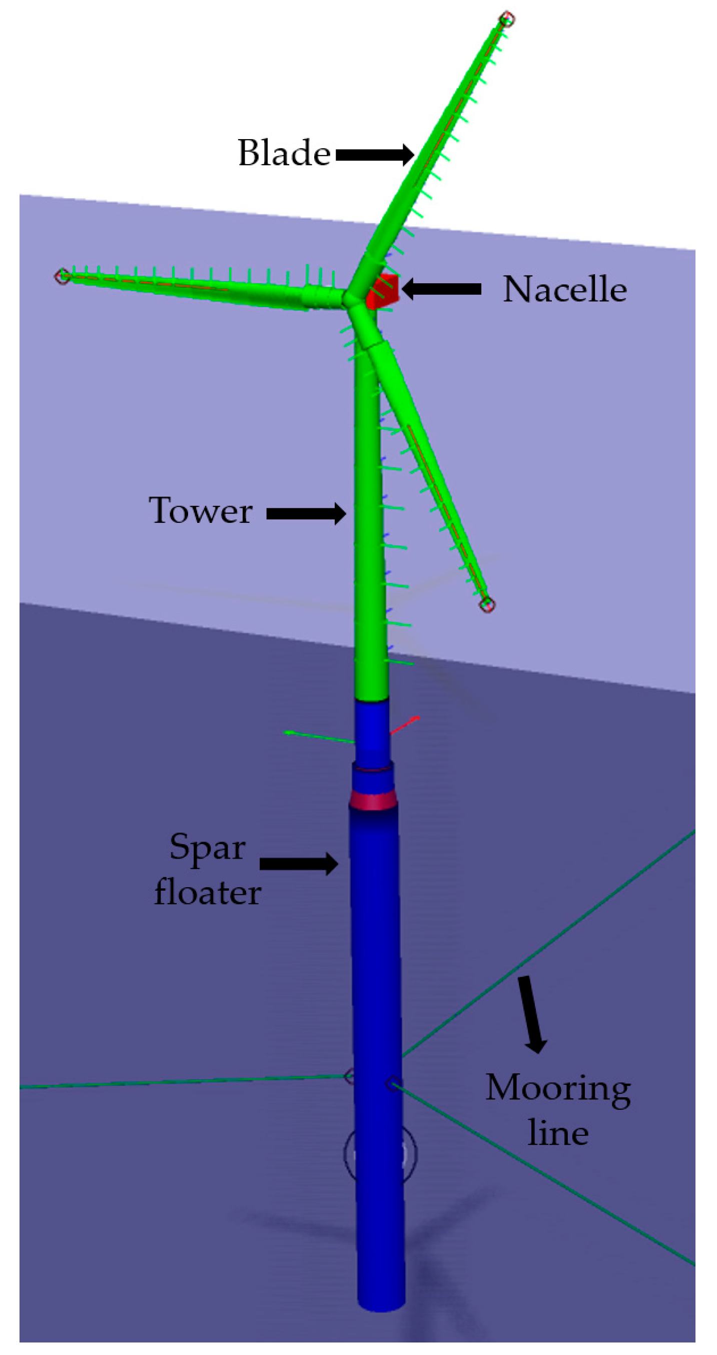
A floating spar wind turbine was selected for this study, which is based on the International Energy Agency (IEA) Annex XXIII Offshore Code Comparison Collaboration (OC3) Phase IV [21]. The OC3 wind turbine has the 5 MW National Renewable Energy Laboratory (NREL) reference wind turbine (RWT) characteristics with a modified controller to prevent the negative damping effect (excessive motions) of the spar platform [21]. The main characteristics of the OC3 wind turbine are provided in Table 2, while the detailed specifications can be found in Jonkman and Musial [21]. Time domain simulations are performed in this study, where the Simulation Workbench for Marine Applications (SIMA) [22], specifically coupled SIMO-Riflex, is used as the primary simulation tool to obtain the OC3 wind turbine’s structural responses and motions. SIMO handles the spar platform’s motions and station-keeping behavior, while Riflex deals with flexible slender structure analysis (i.e., forces, moments, and deflection computation of the turbine’s blades, wind turbine tower, and mooring lines) based on the Finite Element Modeling [22]. Blade Element Momentum (BEM) theory is implemented in Riflex to compute the aerodynamic responses. The modelled OC3 Hywind wind turbine in SIMA is illustrated in Figure 1. The OC3 Hywind is modelled separately for the following parts: blades, nacelle, tower, spar floater, and mooring lines. Each blade is composed with 17 segments representing different airfoil cross-sections of the NREL 5 MW RWT, while the nacelle is modelled as a body. The tower is made up by 10 segments for each of the tower’s cross-section properties, in accordance with Jonkman and Musial [21]. The spar floater is modelled as a body and its hydrodynamic properties are taken from Jonkman and Musial [21].
As input to SIMA, environmental conditions are necessary, where waves and wind act as the main environmental loads. The waves’ input are taken as constant for all load cases considered in this study, while the wind input defines the load cases. The simulated wave conditions follow a Joint North Sea Wave Project (JONSWAP) spectra with a significant wave height of Hs = 4 m, peak period Tp = 8 s, and a peakedness parameter γ = 3.3, according to DNVGL-CG-0130 [23]. In reality, Hs is dependent on wind speed and should be varied. Additional simulations were performed with variable Hs and Tp. It was noted that simulations with a variable Hs yield similar conclusions (in terms of the OC3 Hywind’s responses with respect to the variation in wind input), as to when a constant Hs is adopted. Since our main objective is to investigate the impact of wind input variation on the OC3 wind turbine’s responses, a constant Hs with wind speed is used in this study.
The main input for the simulations in SIMA is wind inflow conditions (wind fields) that is depicted in the form of ‘moving wind box’ in the u-component direction. This box will be referred to as the turbulence box. The turbulence boxes are pre-generated using different pre-processing tools depending on the wind model. TurbSim [19] is used to generate the turbulence box using the Kaimal Model, Mann Turbulence Generator (MTG) [24] for the Mann spectral model, and windSimFast [25] for the Pointed-Blunt model, where the windSimFast is a MATLAB®-based code. The turbulence box contains wind velocity values at each grid point, representing the flow field variation on the rotor for a selected duration, here taken as 1 hour. The turbulence box size is set to (height × width × length = 160 m × 160 m × [Uhub (mean wind speed at hub) × 3600]). For example, if Uhub is 8 m/s, then the turbulence box size is 160 m × 160 m × 28,800 m. The selected height and width size are to cover the rotor swept area and account for the platform motions. Furthermore, it is important to note that the grids in the turbulence box have proper resolutions. A note on the turbulence box’s grid resolution is given in Section 2.2.1.
The load cases (LC) for this study are summarized in Table 3. The load cases are divided into two main cases, LC 1 and LC 2. LC 1 concerns turbulent wind under neutral conditions with two different coherences and LC 2 covers turbulent wind for different atmospheric stability conditions paired with a fixed exponential coherence.
The turbulence intensity (TI) input values for LC 1 are set equal to the values simulated with the Pointed-Blunt model under neutral stability conditions (LC 2a). Each of the load cases is simulated for 1 hour with six different random seeds to minimize the uncertainty. It is important to note that the 1-hour long time series of the incoming flow are simulated continuously, i.e., not split into 10 min long segments, in order to include the low-frequency wind gusts.
As a simplification, the effect of wind shear is neglected, and a uniform wind profile is applied for all load cases presented in Table 3. Additional simulations were also performed using a stability-corrected logarithmic mean wind profile for all load cases presented in Table 3. For unstable conditions, there is very little wind shear, and as a result, very little influence was noted on the resultant loads and motions of the OC3 Hywind (less than 10%, depending on the component of interest). Whereas for neutral conditions, we observed that the influence of coherence on the OC3 Hywind responses is greater than the variation in mean wind profile. However, since the focus of this study is a comparison of the turbulent wind models, it is then decided to simplify the comparison by using a constant mean wind profile with height.
2.2.1. A Note on the Turbulence Box’s Grid Resolution
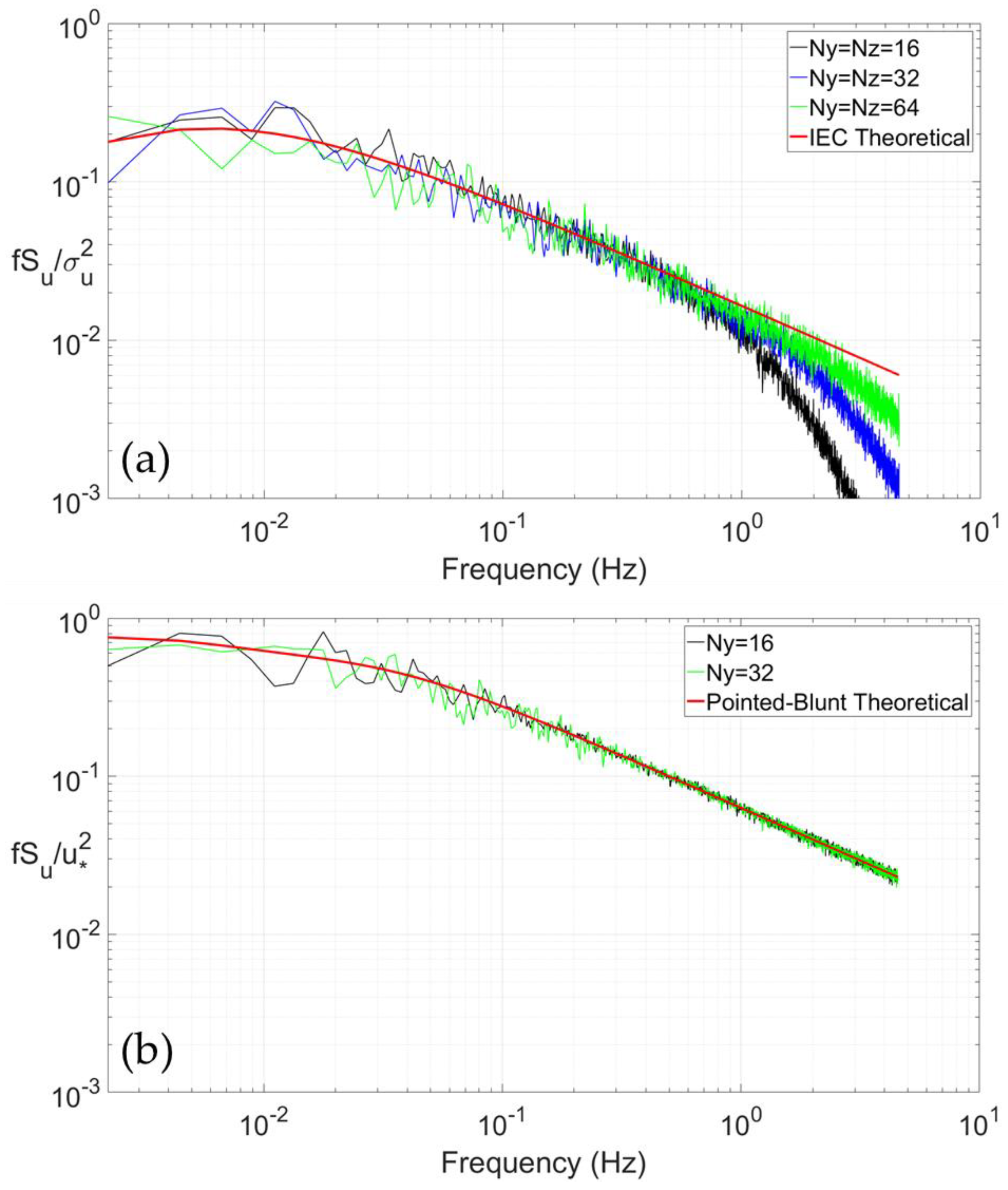
When one uses the MTG, the finding by Kim et al. [26] suggests that grid spacing plays an important role in defining a reliable input, and thus the simulation results. Their study pointed out that coarser grid resolution gives a more biased result compared to the finer grid resolution. Hence, a grid resolution check is performed, particularly for the Mann spectral model where the wind turbulence box is generated using MTG. In MTG, the number of grid points in the x, y, and z directions (Nx, Ny, Nz) must follow 2n, where n is a positive integer. To satisfy this requirement, a number of grid point in the x-direction, Nx = 32,768 is selected, which corresponds to a time step dt of 0.11 s for a 3600 s duration (dt = duration/Nx). Table 4 provides different grid resolutions to be checked. Figure 2a presents the Mann spectral model spectra of the u-component (Su) simulated by the MTG tool for different grid resolutions in Table 4, compared with the target spectra for the Mann spectral model. It can be seen that the variation in grid resolution influences the simulated spectra of the along-wind component Su, particularly at frequencies higher than 0.7 Hz. The simulated spectra Su decays faster than the target spectra at frequencies > 0.7 Hz. The finer grid spacing resulted in simulated spectra Su values closer to the target spectra compared to the coarser grid spacing for frequencies > 0.7 Hz.
The low-pass filtering in the Mann spectral model assumes the grid points as the average wind speeds in a cube volume of air [27]. Even though a high-frequency compensation is applied when using MTG to allow the grid points to represent a local wind vector instead of the air cube, it seems that the low-pass filtering is not well compensated, even for the very fine grid size (see Table 4). A finer grid is then seen to better represent the smaller scale turbulence. When an isotropic grid (dx = dy = dz) was used, we observed that the simulated spectra in the frequency > 0.7 Hz approaches the theoretical spectra (red line in Figure 2a). Ideally, an isotropic grid spacing would give the closest values with the theoretical ones for all frequency ranges and should be used in the simulations. Nonetheless, such grid spacing is quite difficult to consider in the simulations. The number of grids, Nx, Ny, Nz, must follow 2n, and MTG’s computational power is limited. Moreover, if a constant dx is used for a constant duration of 3600 s, then Nx will change with wind speed, Uhub. Hence, the turbulence box size will change with wind speed, Uhub. We aim to have a constant wind field size with a continuous duration of 3600 s and a constant time step dt for all considered wind speeds, Uhub. Because the use of isotropic grid spacing will lead to inconsistent turbulence box size with wind speed, the very fine grid size (Ny = Nz = 64) is then selected for all wind simulations using both MTG and TurbSim. As shown in Figure 2b, the grid resolution does not influence the simulated wind of the Pointed-Blunt model. Therefore, a fine grid size (Ny = Nz = 32) is used to generate the wind turbulence box using windSimFast.
The importance of Nx on the simulated spectra Su is related to the time step dt. Nx variation corresponding to a time step from 0.055 to 0.11 s shortens the x-axis, i.e., a smaller time step captures a longer high-frequency range. To save the computational time, a time step of 0.11 s is used to generate the turbulence boxes using all tools, allowing a Nyquist frequency of 4.55 Hz, adequate to capture the OC3 wind turbine’s important natural frequencies.
3. Results
The results are divided into three subsections: the simulated wind turbulence in terms of wind turbulence box properties for each load case, the natural frequencies of the OC3 wind turbine, as well as the load and platform motion responses.
3.1. Simulated Wind Turbulence
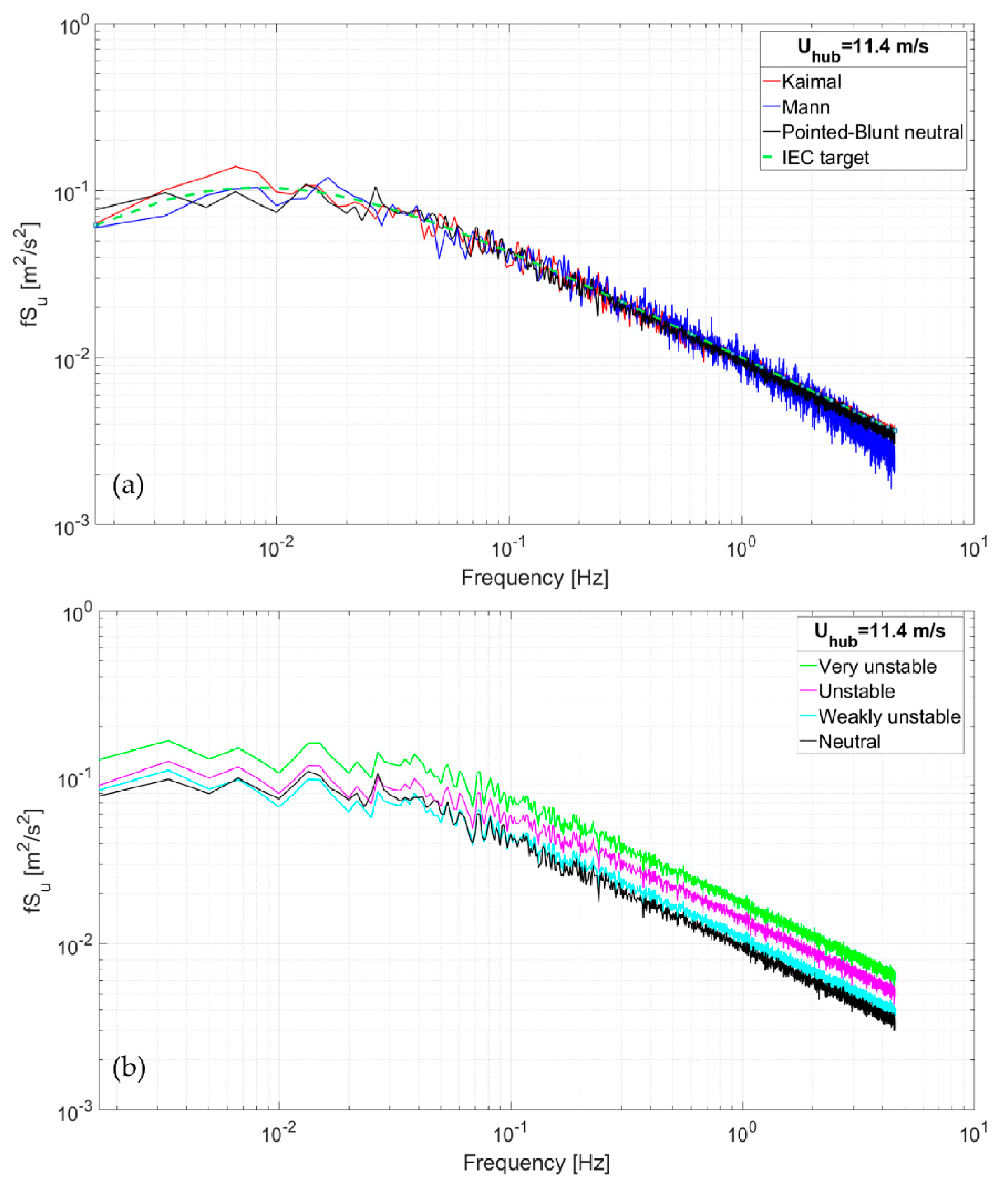
The generated wind turbulence is checked to make sure that its statistical properties meet the required target values. Figure 3a shows the simulated dimensional spectra Su averaged from the six seeds for the Kaimal model and the Mann spectral model in LC 1 compared to the IEC target spectra, as well as the Pointed-Blunt model under neutral conditions (LC 2a). The comparison between the simulated dimensional spectra Su and the theoretical spectra for LC 2 is given in Figure 3b. The spectra shown in Figure 3 are calculated using the Welch’s method with six windows and are plotted as a function of frequency. As shown in Figure 3a, the wind turbulence spectral properties from the Kaimal model and the Mann spectral model agree well with the targeted spectra, except for the Mann spectral model at frequencies > 1 Hz due to the grid size. A good agreement between the simulated spectra and the target spectra is also observed for the Pointed-Blunt model for all stability conditions at all considered wind speeds, and for both v- and w- wind components (Sv and Sw, respectively). Figure 3a shows that the Pointed-Blunt model under neutral conditions in LC 2a has equivalent energy content with the two IEC models, as the TI input for the two IEC models are based on the simulated TI from LC 2a. Comparing different atmospheric stability conditions for LC 2, it can be seen from Figure 3b that the spectra Su is increasing as the stability progressively shifts from neutral to very unstable, except in the 0.008 Hz < frequency < 0.05 Hz range, where neutral conditions produced slightly higher spectra Su than for weakly unstable conditions.
Table 5 gives the range of the simulated TI values of u-component from the six seeds. It can be seen that the simulated TI results for the Kaimal model and the Mann spectral model are slightly lower than the target TI given in Table 3. It is important to note that TI is not an input for the Pointed-Blunt model and thus the TI results for the Pointed-Blunt model are due to the changes in Lm and the value of u* in Equation (7). From Table 5, it is noted that the TI is increasing as the atmospheric stability moves from neutral to very unstable conditions. This is expected as unstable conditions have higher spectra energy Su than neutral conditions, as shown in Figure 3.
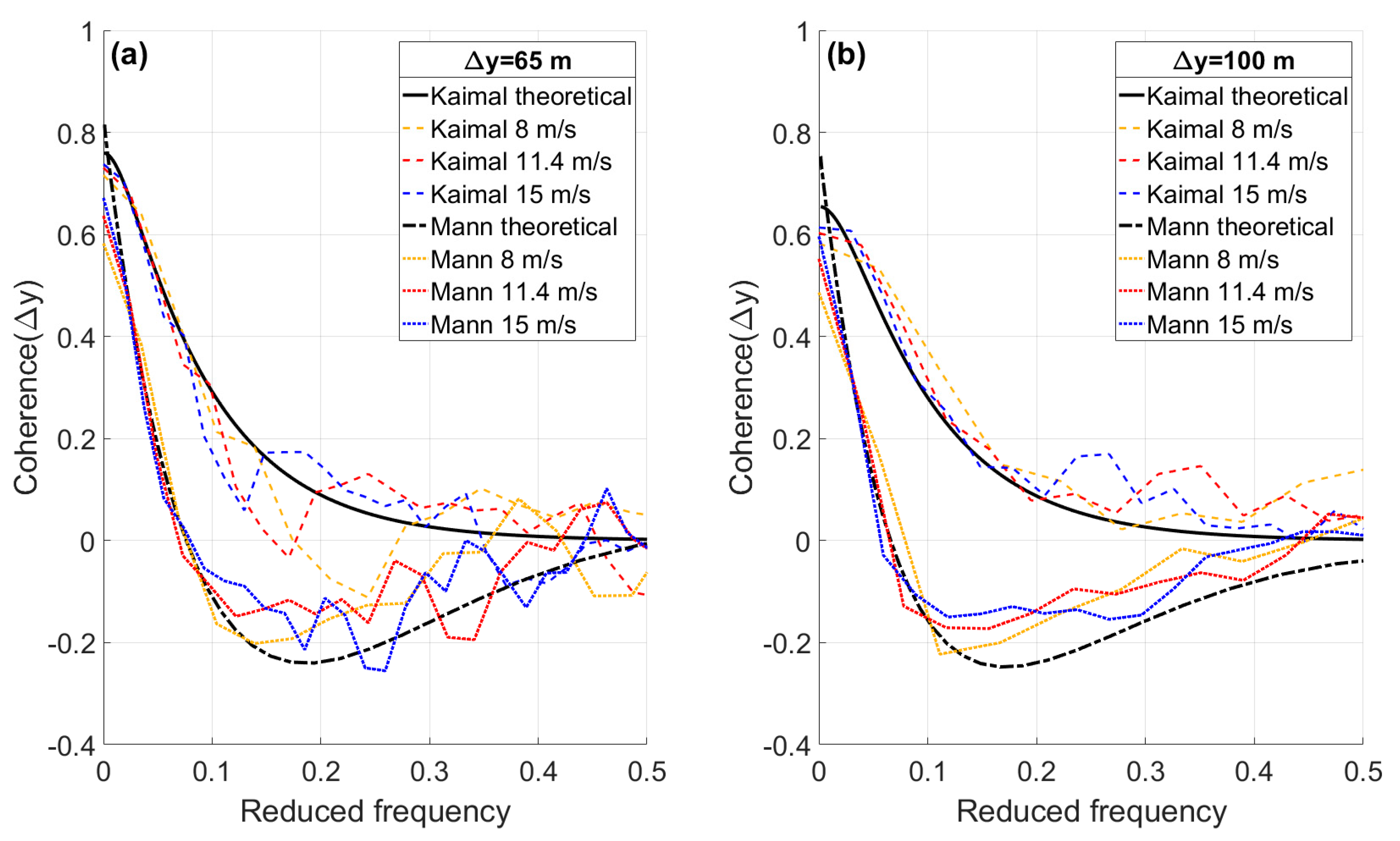
Figure 4 presents the comparison between the simulated wind lateral coherences and the empirical formula (target coherence function) plotted as a function of reduced frequency = f × Δ/Uhub. Where f is the frequency (Hz), Δ is the separation distance (m), and Uhub is the mean wind speed at the hub. The simulated coherences are obtained based on the Kaimal and Mann spectral models for 65 and 100 m lateral separations for all considered wind speeds. As can be seen in Figure 4, the simulated coherences for all wind speeds agree with the target function. We also note this agreement for a small lateral separation of 10 m and for the vertical separations, which are for brevity not presented here. The simulated coherences for the lateral and vertical separations of the Pointed-Blunt model are not shown here but are also observed to be in good agreement with the target exponential coherence function.
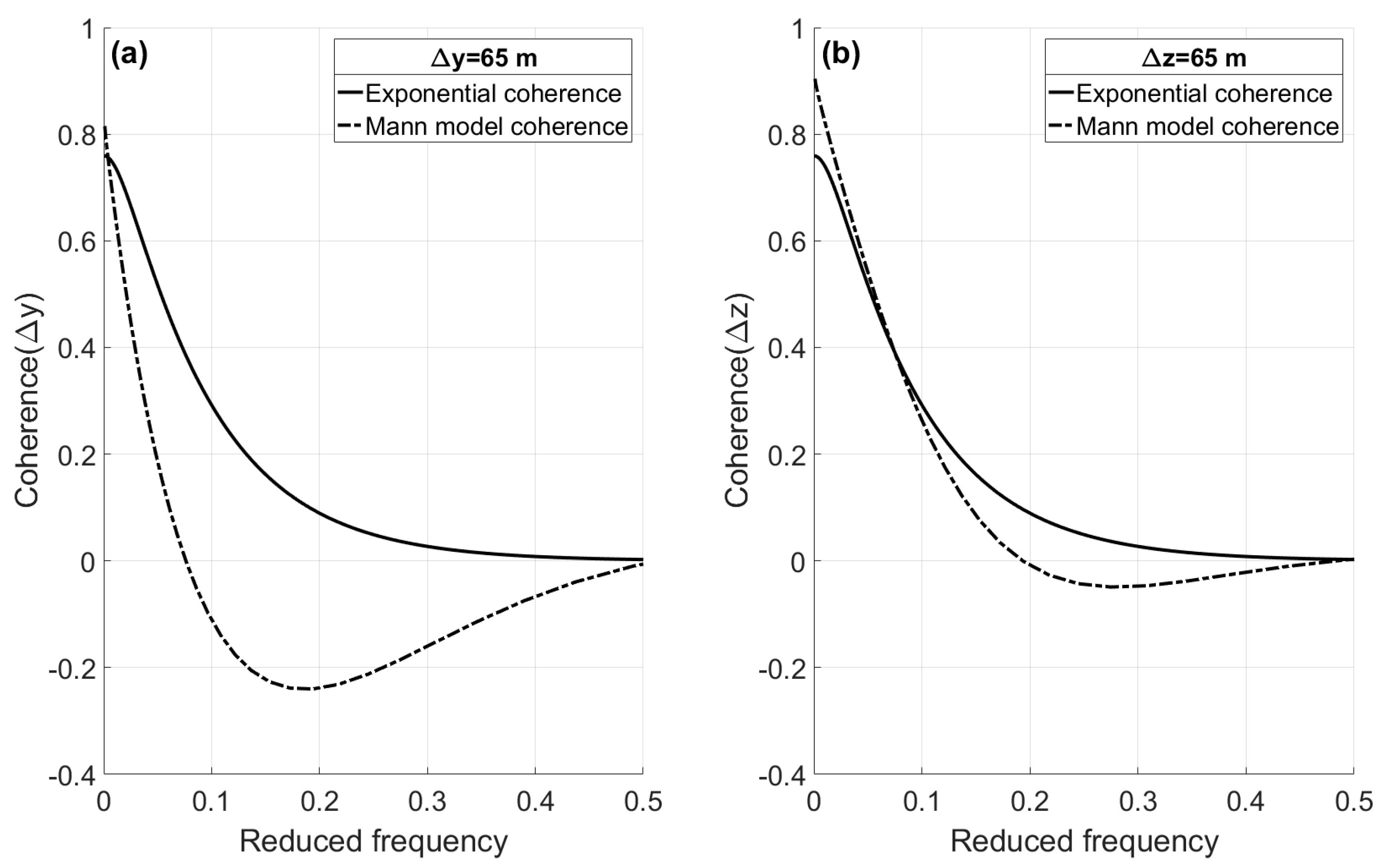
Figure 5 compares the target coherence functions for the exponential coherence model and the Mann spectral model coherence, for the lateral and vertical separations, respectively. In terms of lateral coherence, the Mann spectral model gives lower values than the exponential coherence for the considered reduced frequencies, as shown in Figure 5a. For the vertical coherence, the two coherences are closer to each other, and the one from the Mann spectral model is lower than the exponential coherence for reduced frequencies higher than 0.075 (Figure 5b).
3.2. Natural Frequencies
Free decay tests are performed in SIMA to obtain the natural frequencies of the OC3 Hywind. This is done by considering no wind and still water (no waves) conditions in the simulations. The natural frequency for the OC3 Hywind’s first eight modes is given in Table 6. The values match well with the values obtained in the OC3 code comparison study by Jonkman and Musial [21], except for the platform pitch and the first two tower modes. The corresponding natural frequencies obtained in the study by Saccoman [28] by using Horizontal Axis Wind turbine simulation Code 2nd generation (HAWC2) numerical simulation [24] are also presented in Table 6. It can be seen that the platform pitch and the first two tower modes’ natural frequencies from our study are close to those by Saccoman [28]. The pitch natural frequency of 0.033 Hz as in the present study was also computed by Ahn and Shin [29] using FAST aeroelastic tool [30]. It is important to note that the OC3 Hywind’s natural frequency presented in Table 6 is far lower than the frequency region affected by the grid resolution as discussed in Section 2.2.1.
3.3. Load and Motion Responses
The output from the SIMA simulations are the stress-resultant time series (force, torsional moment, bending moment) for different components as well as motion response time series. The OC3 wind turbine load responses are quantified in terms of fatigue damage, while the platform motion responses are presented in the form of minimum and maximum values from the 6 seeds, and the averaged standard deviation from the six seeds. To quantify the fatigue, the rain flow counting method [31] is adopted by transforming the load response time series into Damage Equivalent Load (DEL). The DELs are then computed using:
where:
DEL = (ΣNiSti m/neq)1/m
- DEL: damage equivalent load,
- Ni: total number of cycles causing failure in bin i from rain flow counting,
- Si: load magnitude causing failure in bin i from rain flow counting,
- neq: equivalent number of cycles,
- m: Wöhler exponent (taken as 3 for steel material and 12 for fiberglass).
The DEL is quantified in 1 Hz duration, so neq is set as 3600 to represent the simulation duration of 1 hour. The DELs from each turbulent wind load case are computed and compared for the following resulting moments of the OC3 wind turbine: tower base fore–aft bending, tower base side–side bending, tower base torsional, tower top torsional, and blade root flap-wise bending. The load and motion responses are discussed separately in two different subsections. The first one is the load and motion responses from LC 1, where turbulent wind under neutral conditions with different coherences are compared. Secondly, the load and motion responses from LC 2, where turbulent wind under different atmospheric stability conditions, from neutral to very unstable, are described.
3.3.1. Influence of Coherences under Neutral Atmospheric Stability Conditions
The OC3 wind turbine responses with respect to variation in the coherence under neutral conditions (LC 1) show that the tower base side–side moment, the tower top torsional moment, and the tower base torsional moment are the most affected components. It is observed that the Mann spectral model results in up to 27%, 20%, and 20% higher DELs than the Kaimal model respectively, for the aforementioned components at the highest considered wind speed 15 m/s (see Figure 6 for torsional moment). In contrast, the tower base fore–aft moment and the blade root flap-wise moment are not significantly affected by the variation in coherence under neutral conditions. The Mann spectral model yields 2% higher DELs for the tower base fore–aft moment and 5% lower DELs for the blade root flap-wise moment. The small difference in the blade root flap-wise moment responses associated with the two different spectral models are consistent with the uniform wind profile that is adopted for all cases in LC 1. Sathe and Bierbooms [32] showed that the mean wind shear profile governs the blade loads. The uniform mean wind profile, accompanied by a uniform TI with height (the numerical simulations of a flow field with nominally uniform turbulence intensity of, for example, 5.95%, result in a variation of turbulence intensity of about 0.5% across the rotor area, both for the Kaimal model and the Mann spectral model flow fields. Such variations in the simulated flow characteristics across the rotor area are considered to be of a secondary importance for the studied wind turbine responses), and the fact that turbulence correlation over smaller distances (than those relevant for the tower twisting and yawing) dominates the dynamic loading of a single blade, all contribute to a limited influence on the blade root flap-wise responses in the present study.
The tower base fore–aft moment response is the least influenced by variation in the coherences comparing the Kaimal model and the Mann spectral model. This is consistent with a small difference in vertical coherence between the two models, as shown in Figure 5b. In contrast to this, the different vertical coherences for different atmospheric stability conditions were found to give 75% difference in the tower base fore–aft loads for a bottom-fixed wind turbine [9]. A further investigation of the influence of the representative, stability dependent vertical coherence on the tower fore–aft response of a floating wind turbine is however needed to examine this and is not discussed in the present study. On the other hand, the tower base side–side responses vary greatly with the difference in the coherences, where a lower coherence produced a 27% higher response, which might be caused by the induced tower base torsional moment.
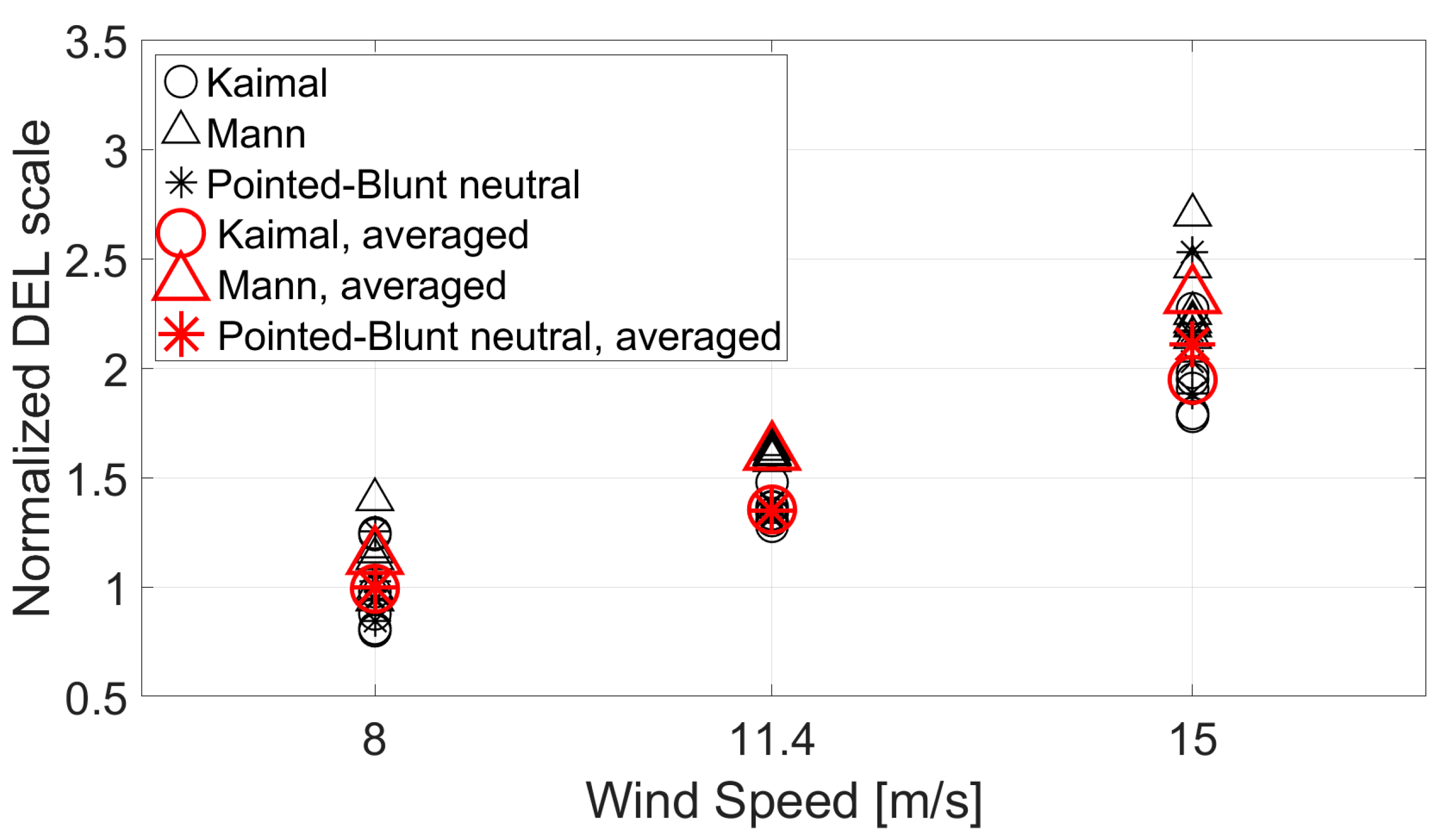
Since the characteristic of the tower top and the tower base torsional moments are alike, only the tower top torsional moment is discussed in the following. Figure 6 presents the normalized DELs for the tower top torsional moment for the Kaimal model and the Mann spectral model in LC 1 and the Pointed-Blunt model under neutral conditions in LC 2a. The DELs are normalized with the values from LC 2a at 8 m/s. The tower top torsional moment DELs are increasing significantly with wind speed, as shown in Figure 6. The difference in the tower top torsional moment DEL is evident between the Kaimal and Mann spectral models (Figure 6). From Figure 3 and Table 5, we see that the Kaimal and Mann spectral models have approximately equal energy content and TI.
The difference in the DEL values is understood to be due to the difference in the coherence functions associated with the Kaimal model and the Mann spectral model, in particular the difference in the lateral coherence (see Figure 4 and Figure 5a). The lower lateral coherence in the Mann spectral model than in the Kaimal model represents less correlated wind gusts at lateral separations, i.e., a higher ‘asymmetry’ of the wind field which then creates higher twisting loads about the wind turbine’s vertical axis. A similar result has also been noted in previous studies [7,8]. Since the Pointed-Blunt model under neutral conditions is used here with the same lateral coherence as for the Kaimal model, the tower top torsional moment responses for the two models are quite similar, as can be seen in Figure 6.
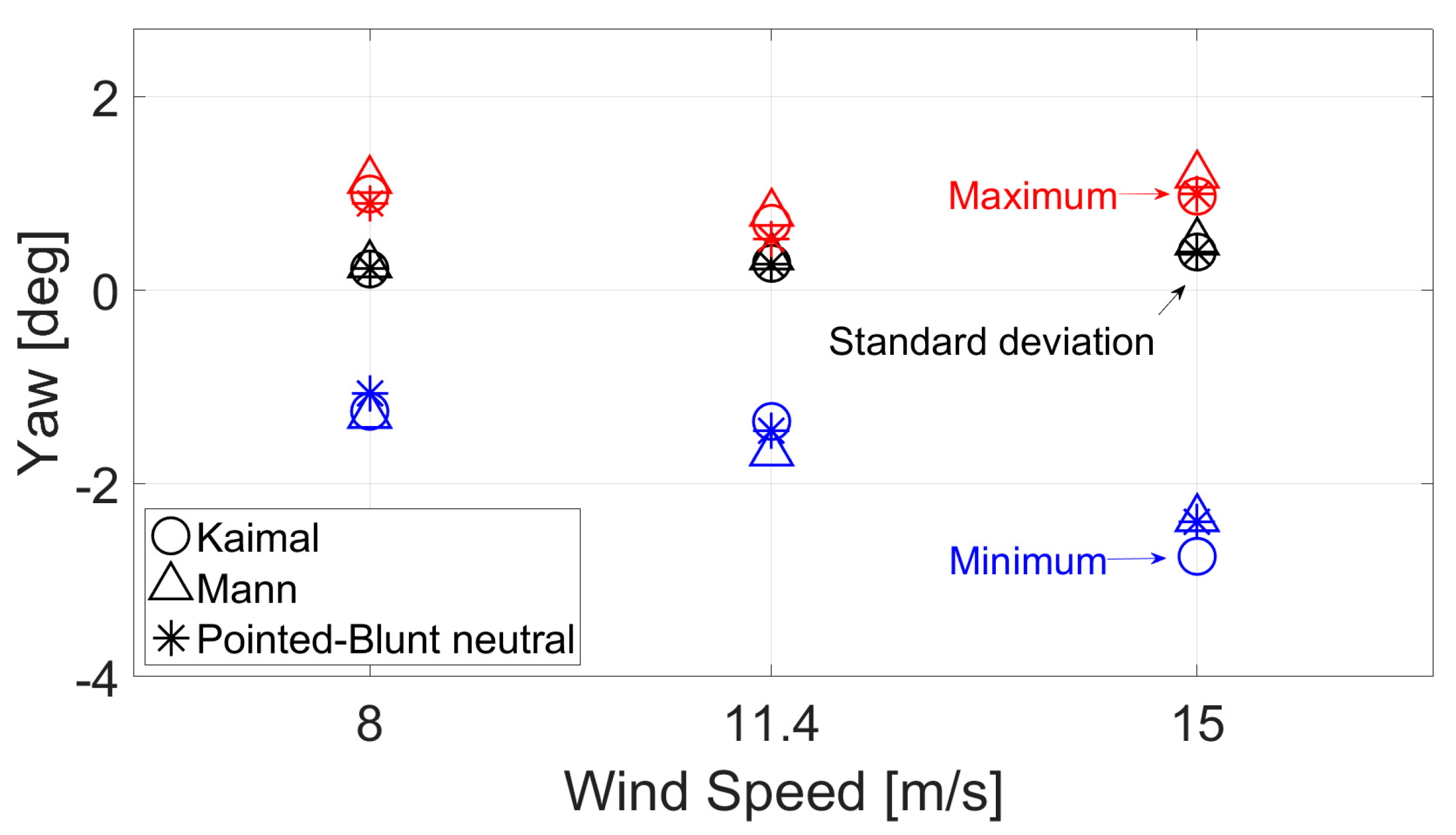
With respect to platform motions, it is found that the platform’s sway, roll, and yaw are the most affected responses by the differences in the coherence functions. The platform sway and roll are of relatively small magnitude, between −1.3 to +0.6 m for sway and −0.3 to +0.6° for roll at the highest wind speed. The platform yaw is in the range of −2.7 to +1.1° for LC 1 at the highest wind speed investigated, as shown in Figure 7. The standard deviations of the platform yaw resulted from the Kaimal model and the Pointed-Blunt model LC 2a are similar, while the yaw response associated with the Mann spectral model is slightly higher than the two, by 0.1 at 15 m/s wind speed (Figure 7). This is due to the Kaimal model and the Pointed-Blunt model LC 2a that have the same lateral coherences, higher than the lateral coherence of the Mann spectral model. The lower lateral coherence by the Mann spectral model causes a higher twisting moment about the wind turbine’s vertical axis and thus induces a higher yaw motion of the floater.
In general, the variation in platform yaw with different turbulent wind conditions in LC 1 shows similar trends with the increase in mean wind speed as the tower top torsional moment DELs (see Figure 6 and Figure 7). This demonstrates the interdependency between the tower torsional moment and the platform yaw response. The platform surge shows a limited sensitivity to the difference in coherences between the Kaimal model and the Mann spectral model. The platform surge is mainly influenced by the thrust on the rotor, which depends greatly on the mean wind speed. The same is observed for platform pitch motion which largely follows the effect of thrust force [33]. For a spar-type wind turbine, the influence of wave conditions on the heave response is more pronounced than the influence of turbulent wind [7]. The observed insignificant response of the platform heave with the difference in the coherences is due to the wave conditions that are kept constant.
Figure 8 presents a segment of the simulated time series of the tower top torsional moment and the yaw response from the Mann spectral model. It can be seen that, generally, the platform yaw angle and the tower top torsional moment are highly correlated. The computed correlation coefficients between the tower torsional moment and the platform yaw are in the range of 0.55 to 0.8.
The snapshots of the underlying wind velocity fluctuations across the rotor are also included, for a case of large and small twisting moment. The moments are seen to be associated with the asymmetrical and the symmetrical distribution of the wind velocity fluctuation over the rotor, with respect to the vertical line y = 0 m. A ‘differential’ action of wind gusts corresponding to an asymmetric field distribution leads to an extreme yaw response of the OC3 wind turbine, in line with the previous discussion. A uniform, symmetric distribution of wind fluctuation over the rotor has an opposite effect.
3.3.2. Influence of Variation in the Atmospheric Stability Conditions
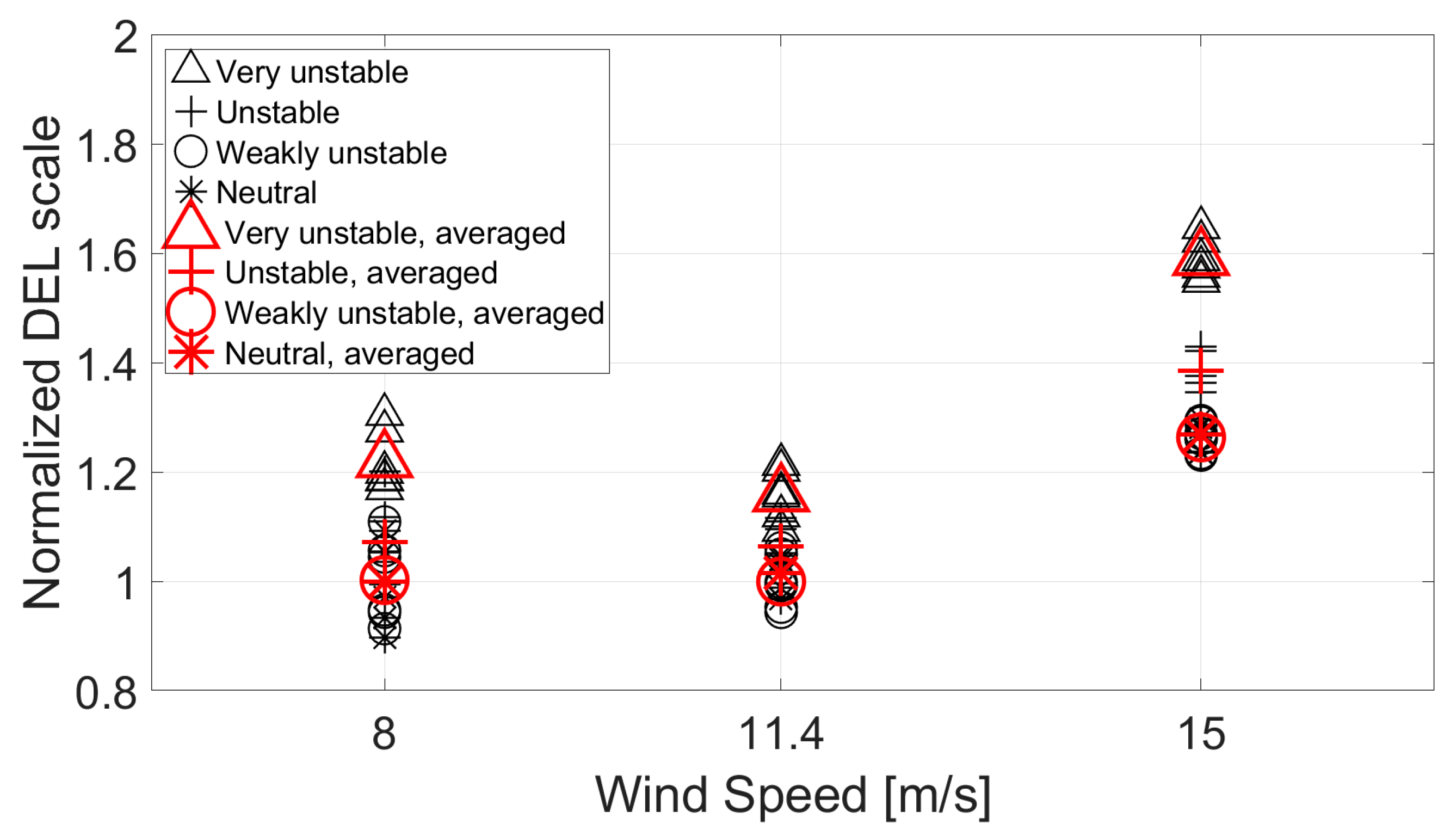
For different atmospheric stability conditions, the tower base side–side moment, the tower top torsional moment, and the tower base torsional moment of the OC3 wind turbine are found to be the most affected components. In LC 2, the wind loads associated with the very unstable conditions result in 27%, 27%, and 26% higher DELs than with the neutral conditions respectively, for the aforementioned components. The DELs of the three most affected component are highest under very unstable conditions, followed by unstable, and then weakly unstable and neutral conditions with close values (less than 3% difference). This is explained by the highest wind energy content under very unstable conditions, followed by unstable, and then weakly unstable and neutral conditions with close values (see the spectra in Figure 3b and the TI values in Table 5 for LC 2). The higher the energy content, then the higher the resultant TI level, and therefore results in higher tower base side–side moment, the tower top torsional moment, and the tower base torsional moment responses. Similar results were shown in previous studies [14,15].
On the other hand, the tower base fore–aft moment and the blade root flap-wise moment are not significantly affected by the variation in turbulent wind input for progressively more unstable conditions. Very unstable conditions yield 4% and 3% higher DELs compared to those under the neutral conditions for the tower base fore–aft moment and the blade root flap-wise moment, respectively. The blade root flap-wise moment response is the least influenced by the difference in stability conditions, similar to the results in the above analysis of the wind load conditions in LC 1. The small difference in the tower base fore–aft moment response by comparing different stability conditions is due to the fact that the tower base fore–aft response is mainly influenced by the spar platform’s surge and pitch motion, that are predominantly affected by the considered waves. Since a constant wave input is considered for all cases in LC 2, we observe an insignificant response change in the tower base fore–aft response with respect to the difference in turbulent wind energy content.
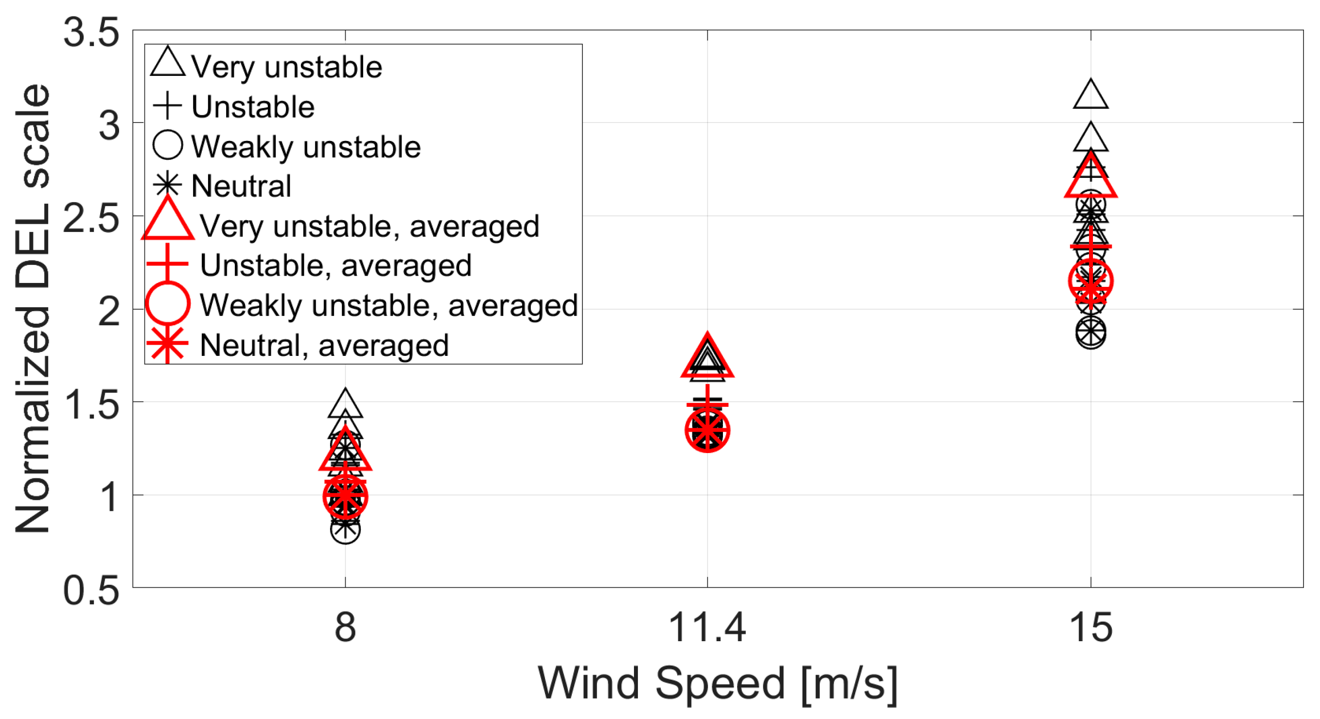
Figure 9 and Figure 10 show the tower top torsional moment and the tower base side–side moment normalized DELs respectively, for different stability conditions. The DELs are normalized with the DEL values obtained for neutral conditions (LC 2a) at 8 m/s. The tower top torsional moment DELs are increasing with wind speed (Figure 9) and so is the tower base side–side moment DELs (Figure 10).
The normalized tower top torsional DEL values as associated with the Mann spectral model LC 1b (Figure 6) appear to be ‘catching up’ with the resulting DEL values from the Pointed-Blunt model LC 2c (Figure 9), even though the LC 1b under neutral conditions has a somewhat lower TI level than the unstable conditions in LC 2c (Table 5). The Pointed-Blunt model for all stability conditions is simulated with a fixed exponential coherence, with a higher lateral coherence level than the Mann spectral model, as shown in Figure 4. As a result, the Mann spectral model wind fields are more ‘asymmetrical’ relative to the Pointed-Blunt wind fields and result in a twisting moment about the wind turbine’s vertical axis that is comparable with the Pointed-Blunt model for unstable conditions with higher TI.
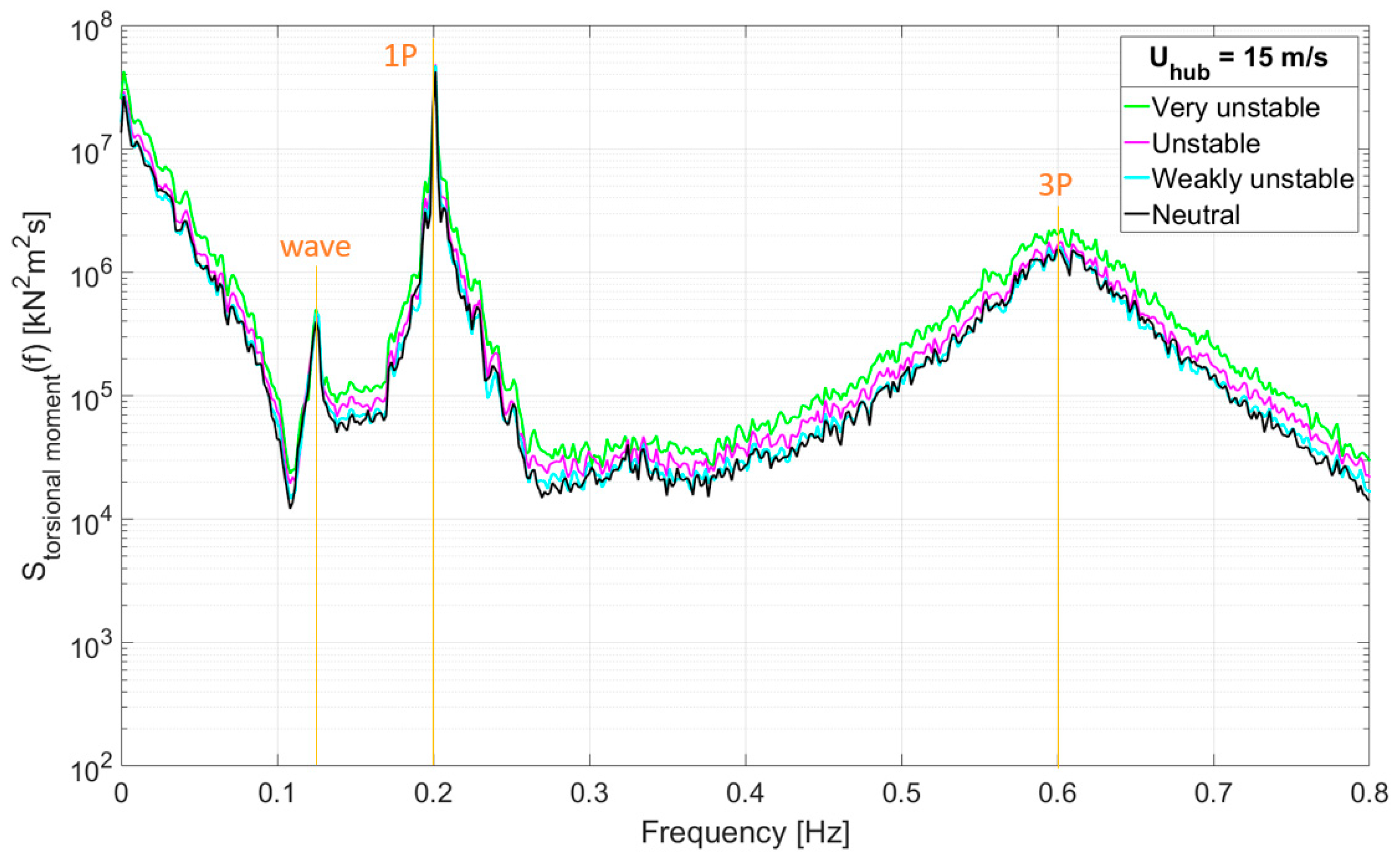
The average power spectral density (PSD) from the six simulated seeds of the tower top torsional moment response for different stability conditions in LC 2 are presented in Figure 11. The tower top torsional moments are the highest under very unstable conditions, followed by unstable conditions, then weakly unstable and neutral conditions with a small discrepancy, as expected. This agrees with the DEL trend presented in Figure 9 for the tower top torsional moment. The major excitation frequencies for the tower top torsional moment are the wave peak frequency, the blade passing 1P frequency, and the blade passing 3P frequency. The wave excitation in the tower top torsional moment response might be due to the platform yaw natural frequency (0.12 Hz) that is excited by the wave peak frequency at around 0.125 Hz. Therefore, we observed the wave excitation in the tower top torsional moment response due to the interdependency between the tower top torsional moment and the platform yaw response. However, the contribution of the excitation blade passing frequencies, 1P and 3P to the tower top torsional moment is higher than that of the wave excitation. This agrees with the findings in References [7,34]. Furthermore, the low-frequency wind excitation (less than 0.1 Hz) is also seen to generate an important part of the torsional moment variations. This indicates the importance of precise description of wind inflow conditions on the rotor of a spar wind turbine, as the rotor harmonics appears to significantly affect the tower torsional moment response.
In terms of platform motions, it is found that the platform’s sway, roll, and yaw are the most sensitive to the variations in the atmospheric stability conditions in LC 2. The platform sway and roll are of relatively small magnitude, between −1.4 to +0.65 m for sway and −0.3 to +0.63° for roll. The platform yaw is in the range of −2.9 to +1.1° for LC 2 at the highest wind speed investigated, as shown in Figure 12. The platform yaw shows similar trends with the increase in mean wind speed for different stability conditions as the tower top torsional moment DELs (see Figure 9 and Figure 12). Again, this indicates the related excitation mechanisms for both the tower torsional moment and the platform yaw response. The platform yaw standard deviation is the highest under very unstable and the lowest under neutral conditions, with the latter result being close to that for weakly unstable conditions. The platform surge and pitch are found to be driven by the wave conditions which are not varied in the present study. In the frequencies 0.033 Hz < f < 0.07 Hz, we note the highest surge and pitch spectral energy under very unstable conditions, which decreases as the stability shifts to neutral conditions with small discrepancies. In the wave excitation frequency (0.125 Hz) to 0.3 Hz, no spectral energy discrepancies are observed and the spectral energy under all stability conditions coincides with each other. The same is noted for the platform heave, which is, again, more prone to the variation in wave conditions [7], which are not varied in the present study.
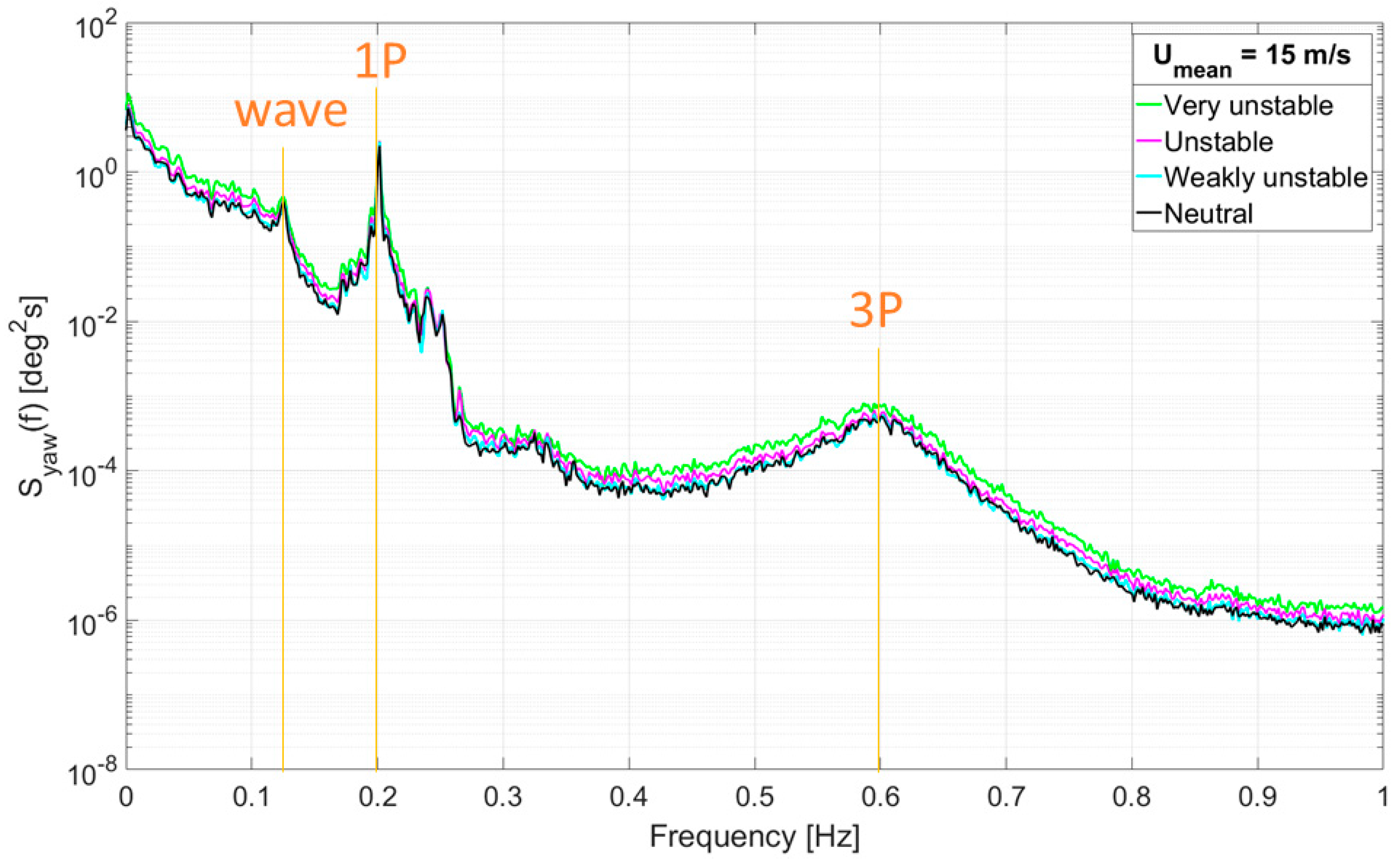
Figure 13 shows the average PSD of the platform yaw response from the six simulated seeds, for different stability conditions in LC 2. It can be seen that the platform yaw responses are the highest under very unstable conditions and decrease as the stability changes to neutral conditions. The platform yaw is mainly excited by the low-frequency turbulence, the wave excitation, and the blade passing 1P and 3P frequencies. The wave excitation in the platform yaw response might be because the platform yaw natural frequency (0.12 Hz) has a very close value with the wave peak frequency (0.125 Hz). Nonetheless, the 1P excitation gives a higher contribution than the wave excitation.
4. Conclusions
The present study was motivated by previous studies [6,7,8] which suggest that the wind spatial coherence is an important factor to consider when simulating the motions of a spar floating wind turbine. In addition, Putri et al. [14] demonstrated the importance of unstable atmospheric conditions for a spar floating wind turbine’s loads and motions. Through SIMA simulations and relevant wind turbulence simulation tools, the influence of different turbulent wind conditions on the OC3 wind turbine loads and motions was investigated. The primary objectives of the study were to clarify how the two turbulent wind models given in the IEC standards result in different stress resultants and motion responses of the OC3 wind turbine, even though both models imply the same energy content for neutral atmospheric stability conditions for a single point spectra. The difference in the spatial coherence between the two models was demonstrated as the main cause for the differences in the wind turbulence load effects on the OC3 turbine. The importance of defining the appropriate coherence for offshore conditions was thus highlighted. The coherence functions of the Kaimal and Mann spectral models for neutral atmospheric stability gave different levels of frequency-dependent correlation of wind gusts, particularly for the across-flow, lateral separations. The lower lateral coherence simulated by the Mann spectral model resulted in higher tower top torsional moments and tower base side–side moments than the Kaimal model by 20% and 27%, respectively.
Additionally, we aimed to demonstrate the impact of the energy level and turbulence content, related to the non-neutral atmospheric stability, especially unstable conditions on the OC3 wind turbine load and motion responses. This was performed by using the Pointed-Blunt spectral model, which was previously derived from FINO1 wind measurement data. The observed increase in the simulated DELs as the atmospheric stability shifts from neutral to very unstable was strongly correlated with the increase in the turbulent wind energy content, and thus the respective increase in TI. The simulated DEL values for tower top torsional moment and tower base side–side bending moment under very unstable conditions were 27% and 26% higher than the values under neutral conditions.
The two aspects of the turbulent wind field, the coherence and the energy content, were studied by changing each aspect at the time. Different flow characteristics were simulated without considering the variations with height. Such idealized flow fields are suited to identify the importance of each aspect of the turbulent flow field, rather than to fully represent conditions in a wind field.
The same exponential coherence was assumed for uu-, vv-, and ww- components due to the absence of relevant information. We also ran simulations with the Kaimal spectral model by using the same exponential coherence for uu- (Equation (2)) but applying identity coherence for vv- and ww- (as suggested by Jonkman [19]). This case resulted in only 2% smaller DEL values than the values presented in this study, depending on the component of interest. The coherence functions for the vv- and ww- components adopted in the present study are hence considered plausible and suitable for the analyses carried out.
The variation in the spatial coherences for different atmospheric stability conditions was not considered in the present study. Instead, fixed coherence values for different atmospheric stability conditions were assumed due to the absence of a valid lateral coherence under non-neutral conditions. The study by Doubrawa et al. [8] showed that the lateral coherences obtained from LES might be sensitive to the change in atmospheric stability conditions only at frequencies lower than 0.1 Hz and separations higher than 140 m for 8 m/s wind speeds. In other words, generally, the lateral coherences yielded from LES under neutral, stable, and unstable conditions are relatively similar, except at the mentioned separations. Therefore, the assumption of pairing a fixed coherence to the Pointed-Blunt model under different unstable conditions in this study could be reasonable. A campaign attempting to acquire the spatial wind coherence information with respect to atmospheric stability conditions from the wind measurements at Obrestad site is currently on-going, but the results are yet to be published [35]. This data can potentially be used for future work.
The present study does not aim to highlight a particular turbulent wind model to predict the accurate responses of a floating wind turbine using numerical simulations. The use of reliable site-specific measured wind data to simulate the wind fields as input into numerical simulations is necessary to get an accurate structural response prediction. Alternatively, the use of LES to simulate the wind fields might also be an option, as demonstrated in the study by Doubrawa et al. [8].
Author Contributions
Conceptualization, R.M.P., C.O., J.B.J. and M.C.O.; data curation, R.M.P.; formal analysis, R.M.P., C.O. and J.B.J.; investigation, R.M.P. and C.O.; methodology, R.M.P.; software, R.M.P.; supervision, C.O., J.B.J. and M.C.O.; visualization, R.M.P.; writing—original draft preparation, R.M.P.; writing—review and editing, C.O., J.B.J. and M.C.O. All authors have read and agreed to the published version of the manuscript.
Funding
This research received no external funding.
Acknowledgments
The authors would like to express their sincerest gratitude to Etienne Cheynet for the support and knowledge provided.
Conflicts of Interest
The authors declare no conflict of interest.
References
- IEC. Wind Turbines–Part 1: Design Requirements; IEC: Geneve, Switzerland, 2005. [Google Scholar]
- Kaimal, J.C.; Wyngaard, J.C.; Izumi, Y.; Coté, O.R. Spectral Characteristics of Surface-layer Turbulence. Q. J. R. Meteorol. Soc. 1972, 98, 563–589. [Google Scholar] [CrossRef]
- Mann, J. The spatial structure of neutral atmospheric surface-layer turbulence. J. Fluid Mech. 1994, 273, 141–168. [Google Scholar] [CrossRef]
- Eliassen, L.O.; Obhrai, C. Coherence of Turbulence Wind under Neutral Wind Condition at FINO1. Energy Procedia 2016, 94, 388–398. [Google Scholar] [CrossRef] [Green Version]
- FINO1–Research Platform in the North and Baltic Seas No. 1. Available online: https://www.fino1.de/en/ (accessed on 27 December 2019).
- Godvik, M. Influence of Wind Coherence on the Response of a Floating Wind Turbine. In Proceedings of the NORCOWE Science Meets Industry, Stavanger, Norway, 6 April 2016. [Google Scholar]
- Bachynski, E.E.; Eliassen, L. The Effects of Coherent Structures on the Global Response of Floating Offshore Wind Turbines. Wind Energy 2019, 22, 219–238. [Google Scholar] [CrossRef]
- Doubrawa, P.; Churchfield, M.J.; Godvik, M.; Sirnivas, S. Load Response of a Floating Wind Turbine to Turbulent Atmospheric Flow. Appl. Energy 2019, 242, 1588–1599. [Google Scholar] [CrossRef]
- Sathe, A.; Mann, J.; Barlas, T.; Bierbooms, W.A.; Van Bussel, G.J. Influence of Atmospheric Stability on Wind Turbine Loads. Wind Energy 2013, 16, 1013–1032. [Google Scholar] [CrossRef]
- Krogsæter, O.; Reuder, J. Validation of Boundary Layer Parameterization Schemes in the Weather Research and Forecasting (WRF) Model under the Aspect of Offshore Wind Energy Applications—Part II: Boundary Layer Height and Atmospheric Stability. Wind Energy 2014, 18, 1291–1302. [Google Scholar] [CrossRef] [Green Version]
- Energy, D.W. DTU Vindenergi: Testcenter Høvsøre. Available online: https://www.vindenergi.dtu.dk/test-centers/hoevsoere_dk(accessed on 7 June 2019).
- Cheynet, E.J.; Jakobsen, J.B.; Reuder, J. Velocity Spectra and Coherence Estimates in the Marine Atmospheric Boundary Layer. Bound. Layer Meteorol. 2018, 169, 429–460. [Google Scholar] [CrossRef]
- Højstrup, J. A Simple Model for the Adjustment of Velocity Spectra in Unstable Conditions Downstream of an Abrupt Change in Roughness and Heat Flux. Bound. Layer Meteorol. 1981, 21, 341–356. [Google Scholar] [CrossRef]
- Putri, R.M.; Obhrai, C.; Knight, J.M. Offshore Wind Turbine Loads and Motions in Unstable Atmospheric Conditions. J. Phys. Conf. Ser. 2019, 1356. [Google Scholar] [CrossRef]
- Knight, J.M.; Obhrai, C. The Influence of an Unstable Turbulent Wind Spectrum on the Lodas and Motions on Floating Offshore Wind Turbines. IOP Conf. Ser. Mater. Sci. Eng. 2019, 700. [Google Scholar] [CrossRef]
- Saranyasoontorn, K.; Manuel, L.; Veers, P.S. A Comparison of Standard Coherence Models for Inflow Turbulence with Estimates from Field Measurement. J. Sol. Energy Eng. 2004, 126, 1069–1082. [Google Scholar] [CrossRef]
- Dyrbye, C.; Hansen, S.O. Wind Loads on Structures; John Wiley & Sons Ltd.: West Sussex, UK, 1997. [Google Scholar]
- IEC. Wind Energy Generation Systems–Part 1: Design Requirements; IEC: Geneve, Switzerland, 2019. [Google Scholar]
- Jonkman, J. TurbSim User’s Guide: Version 2.00.00; National Renewable Energy Laboratory (NREL): Golden, CO, USA, 2016.
- Veritas, D.N. Environmental Conditions and Environmental Loads; Det Norske Veritas: Høvik, Norway, 2010; Volume DNV-RP-C205. [Google Scholar]
- Jonkman, J.; Musial, W. Offshore Code Comparison Collaboration (OC3) for IEA Task 23 Offshore Wind Technology and Deployment; National Renewable Energy Laboratory (NREL): Golden, CO, USA, 2010.
- Ocean, S. SIMA. Available online: https://www.sintef.no/en/software/sima/ (accessed on 28 September 2019).
- DNVGL. DNVGL-CG-0130; Wave Loads; DNVGL AS: Høvik, Norway, 2018. [Google Scholar]
- Larsen, T.J.; Hansen, A.M. How 2 HAWC2, the User’s Manual; Department of Wind Energy: Roskilde, Denmark, 2019.
- Cheynet, E. Wind Field Simulation. Available online: https://se.mathworks.com/matlabcentral/fileexchange/50041-wind-field-simulation-the-user-friendly-version (accessed on 19 October 2018).
- Kim, Y.L.; Lutz, T.; Jost, E.; Gomez-Iradi, S.; Muñoz, A.; Méndez, B.; Lampropoulos, N.; Stefanatos, N.; Sørensen, N.N.; Madsen, H.; et al. AVATAR Deliverable D2.5: Effects of Inflow Turbulence on Large Wind Turbines; D2.5; ECN Wind Energy: Petten, The Netherland, 2016. [Google Scholar]
- Energy, D.W. HAWC2 Online Course. Available online: https://windenergy.itslearning.com/ContentArea/ContentArea.aspx?LocationID=29&LocationType=1 (accessed on 12 February 2016).
- Saccoman, M. Coupled Analysis of a Spar Floating Wind Turbine considering both Ice and Aerodynamic Loads. Master’s Thesis, Aalto University, Aalto, Finland, 2015. [Google Scholar]
- Ahn, H.-J.; Shin, H. Model test and numerical simulation of OC3 spar type floating offshorewind turbine. Int. J. Nav. Archit. Ocean Eng. 2019, 11, 1–10. [Google Scholar] [CrossRef]
- Jonkman, J. FAST: An Aeroelastic Computer-Aided Engineering (CAE) Tool for Horizontal Axis Wind Turbines. Available online: https://nwtc.nrel.gov/FAST (accessed on 2 December 2019).
- Tatsuo, E.; Koichi, M.; Kiyohumi, T.; Kakuichi, K.; Masanori, M. Damage evaluation of metals for random or varying loading—Three aspects of rain flow method. Mech. Behav. Mater. 1974, 1, 371–380. [Google Scholar]
- Sathe, A.; Bierbooms, W. Influence of Different Wind Profiles due to Varying Atmospheric Stability on the Fatigue Life of Wind Turbines. J. Phys. Conf. Ser. 2007, 75, 767–780. [Google Scholar] [CrossRef] [Green Version]
- Bachynski, E.E. Fixed and Floating Offshore Wind Turbine Support Structures. In Offshore Wind Energy Technology; John Wiley & Sons Ltd.: West Sussex, UK, 2018. [Google Scholar] [CrossRef]
- Putri, R.M. A Study of the Coherences of Turbulent Wind on a Floating Offshore Wind Turbine. Master’s Thesis, University of Stavanger, Stavanger, Norway, 2016. [Google Scholar]
- Flügge, M.; Heggelund, Y.; Reuder, J.; Godvik, M.; Nielsen, F.G.; Jakobsen, J.B.; Svardal, B.; Cheynet, E.; Obhrai, C. COTUR Measuring Coherence and Turbulence with LIDARs. In Proceedings of the EERA DeepWind, Trondheim, Norway, 16–18 January 2019. [Google Scholar]
Figure 1.
The OC3 Hywind spar wind turbine model in the Simulation Workbench for Marine Applications (SIMA).
Figure 1.
The OC3 Hywind spar wind turbine model in the Simulation Workbench for Marine Applications (SIMA).

Figure 2.
Normalized spectra of the u-component for: (a) the Mann spectral model from the Mann Turbulence Generator, and (b) the Pointed-Blunt model from windSimFast for different grid resolutions with Nx = 32,768 and 8 m/s mean wind speed at the hub point.
Figure 2.
Normalized spectra of the u-component for: (a) the Mann spectral model from the Mann Turbulence Generator, and (b) the Pointed-Blunt model from windSimFast for different grid resolutions with Nx = 32,768 and 8 m/s mean wind speed at the hub point.

Figure 3.
Spectra of the u-component for 11.4 m/s mean wind speed at hub point based on: (a) Kaimal model and Mann spectral model, and (b) Pointed-Blunt model for various stability conditions.
Figure 3.
Spectra of the u-component for 11.4 m/s mean wind speed at hub point based on: (a) Kaimal model and Mann spectral model, and (b) Pointed-Blunt model for various stability conditions.

Figure 4.
Simulated lateral coherences of the u-component for the Kaimal (exponential coherence) and the Mann spectral models for different mean wind speeds at: (a) 65 m separation (rotor radius) and (b) 100 m separation distances.
Figure 4.
Simulated lateral coherences of the u-component for the Kaimal (exponential coherence) and the Mann spectral models for different mean wind speeds at: (a) 65 m separation (rotor radius) and (b) 100 m separation distances.

Figure 5.
Theoretical coherences of the u-component at 65 m separation (rotor radius) distance for: (a) lateral separation and (b) vertical separation comparing the exponential coherence and the Mann spectral model coherence.
Figure 5.
Theoretical coherences of the u-component at 65 m separation (rotor radius) distance for: (a) lateral separation and (b) vertical separation comparing the exponential coherence and the Mann spectral model coherence.

Figure 6.
Normalized Damage Equivalent Loads (DELs) of tower top torsional moment for neutral conditions for the Kaimal and Mann spectral models using standard TI (LC 1) and the Pointed-Blunt model under neutral conditions (LC 2a). The black markers represent seeds while the red markers represent the average value of the six seeds at the respective wind speeds.

Figure 7.
Platform yaw minimum (blue markers), maximum (red markers), and standard deviation (black markers) for the Kaimal and Mann spectral models (LC 1) and the Pointed-Blunt model under neutral conditions (LC 2a).
Figure 7.
Platform yaw minimum (blue markers), maximum (red markers), and standard deviation (black markers) for the Kaimal and Mann spectral models (LC 1) and the Pointed-Blunt model under neutral conditions (LC 2a).

Figure 8.
Wind velocity fluctuations over the rotor (upper figure) and the tower top torsional moment and yaw response (lower figure) for the Mann spectral model at 15 m/s mean wind speed at the hub, in case of a small (a) and large (b) twisting moment. The circle lines represent the rotor swept area.

Figure 9.
Normalized DELs of the tower top torsional moment for different atmospheric stability conditions for the Pointed-Blunt model (LC 2). The black markers represent seeds while the red markers represent the average value of the six seeds at the respective wind speeds.
Figure 9.
Normalized DELs of the tower top torsional moment for different atmospheric stability conditions for the Pointed-Blunt model (LC 2). The black markers represent seeds while the red markers represent the average value of the six seeds at the respective wind speeds.

Figure 10.
Normalized DELs of the tower base side–side moment for different atmospheric stability conditions for the Pointed-Blunt model (LC 2). The black markers represent seeds while the red markers represent the average value of the six seeds at the respective wind speeds.
Figure 10.
Normalized DELs of the tower base side–side moment for different atmospheric stability conditions for the Pointed-Blunt model (LC 2). The black markers represent seeds while the red markers represent the average value of the six seeds at the respective wind speeds.

Figure 11.
Tower top torsional moment power spectral density (PSD) for different stability conditions in LC 2 at 15 m/s mean wind speed at the hub.
Figure 11.
Tower top torsional moment power spectral density (PSD) for different stability conditions in LC 2 at 15 m/s mean wind speed at the hub.

Figure 12.
Platform yaw minimum (blue markers), maximum (red markers), and standard deviation (black markers) comparing the Pointed-Blunt model for different stability conditions (LC 2).
Figure 12.
Platform yaw minimum (blue markers), maximum (red markers), and standard deviation (black markers) comparing the Pointed-Blunt model for different stability conditions (LC 2).

Figure 13.
Platform yaw PSD comparison for the different stability conditions in LC 2 at 15 m/s mean wind speed at the hub.
Figure 13.
Platform yaw PSD comparison for the different stability conditions in LC 2 at 15 m/s mean wind speed at the hub.


Table 1.
Parameters for the Kaimal model [1].
Table 1.
Parameters for the Kaimal model [1].
| Velocity Component | |||
|---|---|---|---|
| 1 (u) | 2 (v) | 3 (w) | |
| σi | σ1 | 0.8 σ1 | 0.5 σ1 |
| Li | 8.1 Λ1 | 2.7 Λ1 | 0.66 Λ1 |
Table 2.
The Offshore Code Comparison Collaboration (OC3) wind turbine general properties [21].
Table 2.
The Offshore Code Comparison Collaboration (OC3) wind turbine general properties [21].
| Properties | Value |
|---|---|
| Power production rating | 5 MW |
| Rotor diameter (hub diameter) | 126 m (3 m) |
| Hub height | 90 m |
| Cut-in, rated, cut-out wind speed | 3, 11.4, 25 m/s |
| Cut-in and rated rotor speed | 6.9, 12.1 rpm |
| Water depth, platform draft | 320 m, 120 m |
| Added mass, drag coefficient | 0.969954, 0.6 |
| Number of mooring lines (angle between adjacent lines), mooring line length | 3 (120°), 853.87 m |
Table 3.
Load case (LC).
| LC No. | Wind Model | Atmospheric Stability Conditions | Coherence Model | Input Parameters |
|---|---|---|---|---|
| 1a | Kaimal | Neutral | Equation (2) | Uhub * = 8 m/s (TI ** = 5.95%) Uhub = 11.4 m/s (TI = 6.08%) Uhub = 15 m/s (TI = 6.16%) |
| 1b | Mann | Equation (5) | ℓ = 42 m, γ = 3.9 Uhub = 8 m/s (TI = 5.95%), αε2/3 = 0.00956 Uhub = 11.4 m/s (TI = 6.08%), αε2/3 = 0.0203 Uhub = 15 m/s (TI = 6.16%), αε2/3 = 0.036 | |
| 2a | Pointed-Blunt | Neutral | Equation (2) | Lm = ∞ (ζ = 0) Lm = −200 m (ζ = −0.407) Lm = −100 m (ζ = −0.815) Lm = −50 m (ζ = −1.63) Uhub = 8, 11.4, 15 m/s |
| 2b | Weakly unstable | |||
| 2c | Unstable | |||
| 2d | Very unstable | |||
* Uhub = mean wind speed at hub, ** TI = turbulence intensity
Table 4.
Convergence study: grid size.
| No. | Grid Size dy * = dz ** (m) | No. of Grid Points in y and z Directions Ny = Nz (–) | Lx = 3600 s × Uhub = Nx × dx *** (m) | Wind Model |
|---|---|---|---|---|
| 1 | 10 (coarse) | 16 | 28,800 | Kaimal 1, Mann 2 |
| 2 | 5 (fine) | 32 | 41,040 | Kaimal 1, Mann 2 |
| 3 | 2.5 (very fine) | 64 | 54,000 | Kaimal 1, Mann 2 |
* grid size in the y-direction, ** grid size in the z direction, *** grid size in the x direction, 1 TurbSim, 2 Mann Turbulence Generator.
Table 5.
Simulated turbulence intensity of the u-component (mean ± variation).
| Turbulence Intensity (%) | ||||||
|---|---|---|---|---|---|---|
| Uhub (m/s) | LC 1 | LC 2 | ||||
| Kaimal | Mann | Pointed Blunt | ||||
| (a) Neutral | (b) Neutral | (a) Neutral | (b) Weakly Unstable | (c) Unstable | (d) Very Unstable | |
| 8 | 5.77 ± 0.17 | 5.83 ± 0.4 | 5.95 ± 0.2 | 6.0 ± 0.23 | 6.51 ± 0.23 | 7.6 ± 0.27 |
| 11.4 | 5.93 ± 0.15 | 5.95 ± 0.4 | 6.08 ± 0.17 | 6.11 ± 0.2 | 6.61 ± 0.2 | 7.74 ± 0.25 |
| 15 | 6.03 ± 0.14 | 6.01 ± 0.35 | 6.16 ± 0.16 | 6.18 ± 0.2 | 6.67 ± 0.2 | 7.83 ± 0.23 |
Table 6.
Natural frequencies of the OC3 wind turbine.
| Mode | Natural Frequency (Hz) | OC3 Code Comparison [21] (in Hz) | Saccoman [28] (in Hz) |
|---|---|---|---|
| Surge | 0.00714 | 0.0085–0.0093 | 0.00776 |
| Sway | 0.0073 | 0.0085–0.0091 | 0.00776 |
| Roll | 0.045 | 0.51–0.55 | 0.0324 |
| Pitch | 0.033 | 0.054–0.057 | 0.0324 |
| Heave | 0.045 | 0.05–0.054 | 0.0305 |
| Yaw | 0.12 | 0.112–0.18 | 0.121 |
| First tower side–side | 0.492 | 0.67–0.7 | 0.448 |
| First tower fore–aft | 0.52 | 0.6–0.71 | 0.464 |
© 2020 by the authors. Licensee MDPI, Basel, Switzerland. This article is an open access article distributed under the terms and conditions of the Creative Commons Attribution (CC BY) license (http://creativecommons.org/licenses/by/4.0/).
Share and Cite
MDPI and ACS Style
Putri, R.M.; Obhrai, C.; Jakobsen, J.B.; Ong, M.C. Numerical Analysis of the Effect of Offshore Turbulent Wind Inflow on the Response of a Spar Wind Turbine. Energies 2020, 13, 2506. https://doi.org/10.3390/en13102506
AMA Style
Putri RM, Obhrai C, Jakobsen JB, Ong MC. Numerical Analysis of the Effect of Offshore Turbulent Wind Inflow on the Response of a Spar Wind Turbine. Energies. 2020; 13(10):2506. https://doi.org/10.3390/en13102506
Chicago/Turabian StylePutri, Rieska Mawarni, Charlotte Obhrai, Jasna Bogunovic Jakobsen, and Muk Chen Ong. 2020. "Numerical Analysis of the Effect of Offshore Turbulent Wind Inflow on the Response of a Spar Wind Turbine" Energies 13, no. 10: 2506. https://doi.org/10.3390/en13102506
Note that from the first issue of 2016, this journal uses article numbers instead of page numbers. See further details here.