A Study of Wind Turbine Performance Decline with Age through Operation Data Analysis


1
Centre for Renewables and Energy, Dundalk Institute of Technology, Dublin Road, A91 V5XR Louth, Ireland
2
Department of Engineering, University of Perugia, Via G. Duranti 93, 06125 Perugia, Italy
3
School of Architecture & the Built Environment, University of Ulster, Belfast BT9 5AG, UK
*
Author to whom correspondence should be addressed.
Energies 2020, 13(8), 2086; https://doi.org/10.3390/en13082086
Submission received: 26 March 2020
/
Revised: 11 April 2020
/
Accepted: 17 April 2020
/
Published: 21 April 2020
(This article belongs to the Special Issue Lifetime Extension of Wind Turbines and Wind Farms)
Abstract
:Ageing of technical systems and machines is a matter of fact. It therefore does not come as a surprise that an energy conversion system such as a wind turbine, which in particular operates under non-stationary conditions, is subjected to performance decline with age. The present study presents an analysis of the performance deterioration with age of a Vestas V52 wind turbine, installed in 2005 at the Dundalk Institute of Technology campus in Ireland. The wind turbine has operated from October 2005 to October 2018 with its original gearbox, that has subsequently been replaced in 2019. Therefore, a key point of the present study is that operation data spanning over thirteen years have been analysed for estimating how the performance degrades in time. To this end, one of the most innovative approaches for wind turbine performance control and monitoring has been employed: a multivariate Support Vector Regression with Gaussian Kernel, whose target is the power output of the wind turbine. Once the model has been trained with a reference data set, the performance degradation is assessed by studying how the residuals between model estimates and measurements evolve. Furthermore, a power curve analysis through the binning method has been performed to estimate the Annual Energy Production variations and suggests that the most convenient strategy for the test case wind turbine (running the gearbox until its end of life) has indeed been adopted. Summarizing, the main results of the present study are as follows: over a ten-year period, the performance of the wind turbine has declined of the order of 5%; the performance deterioration seems to be nonlinear as years pass by; after the gearbox replacement, a fraction of performance deterioration has been recovered, though not all because the rest of the turbine system has been operating for thirteen years from its original state. Finally, it should be noted that the estimate of performance decline is basically consistent with the few results available in the literature.
1. Introduction
The worldwide installed wind capacity has increased rapidly over recent years and decades [1,2]. This has resulted in an ever increasing number of older industrial wind farms, on a global scale, reaching an age where major component replacements and re-powering are on the horizon.
It is remarkable that most of the attention about wind turbines aging regards the reliability [3,4,5] and the failure rates [6], instead of the performance decline. This in some senses is a bit surprising for at least two reasons: all technical systems are subjected to deterioration and there is no theoretical model about wind turbine performance deterioration with time, which is not due only to increasing failure rates but as well to aerodynamic performance and conversion efficiency decline. Therefore, it is necessary to learn from the experience and in particular from the widespread diffusion of Supervisory Control And Data Acquisition (SCADA) data. There is an impressive amount of scientific literature about the use of wind turbine SCADA data for condition monitoring [7], fault diagnosis [8] and also performance monitoring [9,10,11], but operation data, to date, has not been well exploited for the assessment of wind turbine performance deterioration with age.
On these grounds, the present study aims to make a contribution to the objective of a data-driven comprehension of how the performance of wind turbines deteriorate with age.
At present, at the best of authors knowledge, there are three main studies about the subject. In [12], the public data from 282 wind farms sited in United Kingdom are elaborated, covering 1686 farm-years of operation. In this study, wind speed data with high temporal and spatial resolution are used to measure the performance of wind farms by estimating their theoretical potential output over the course of a month and comparing this with the actual reported load factors. The estimate is that the load factor declines by 1.57% per year: over a 20-year lifetime, this corresponds to a 12% reduction and a 9% increase of the electricity cost. Another important consideration from the study in [12] is that this order of magnitude for the performance decline is remarkable but it is not disastrous because it is in line, for example, with gas turbine technology [13]. The study in [14] refers to wind turbines operating in Sweden, constructed before 2007. The methods and the results are different with respect to [12]: it arises that there is a 0.15 capacity factor percentage points per year decline, corresponding to a lifetime energy loss of 6%; this estimate is lower with respect to [12]. In [15], four SCADA-based wind turbine ageing assessment criteria are proposed for measuring the ageing resultant performance degradation of the turbine: they are based on monitoring the power output, the power coefficient, the nacelle vibration and the temperature of key components. The method is applied on data sets from 2015 and 2016 and it is shown to be effective for estimating the aging effect; however, no lifetime estimate of the performance deterioration is proposed.
This work is a collaboration between the Dundalk Institute of Technology and the University of Perugia and it is based on the fact that the Dundalk Institute of Technology installed a 850 kW rated Vestas V52 wind turbine on its campus in October 2005 and this wind turbine is still operating. As discussed in detail in Section 2, in October 2018 the gearbox of the wind turbine reached the end of life and has been replaced after thirteen years of operation. Therefore, the rationale of this study is employing the operation data of the wind turbine for investigating the performance deterioration with age. In addition, since the gearbox has been replaced, a data set is available describing the operation of the wind turbine with a new gearbox installed with no other modifications made to any of the other original principal components.
The objective of this study has been pursued through the use of the most innovative wind turbine performance monitoring techniques. A benchmark data set of one year, describing the wind turbine running in its first years of operation, has been selected for training a Support Vector Machine Regression with Gaussian Kernel [16], whose target is the power output of the wind turbine. Doing this, a reference model is obtained and the performance deterioration is estimated by studying how the residuals between measurements and model estimates change from earlier to later data sets. These kinds of methods have been applied in the wind energy literature for test cases conceptually similar, despite having opposite outcomes (performance improvements, instead of ageing deterioration): wind turbine aerodynamic and-or control technology optimization [17,18,19]. The effective use of these kind of methods for detecting performance changes of the order of few percents of Annual Energy Production has inspired their application for the test case of the present study. The regression method and the data sets available are described in Section 3.
A further study has been included in this work, with a twofold objective: corroborating the results from the Support Vector Regression and providing some indication about the economic impact of the performance degradation and possible strategies for the wind turbine maintenance. A power curve analysis, based on the binning method recommended by the International Electrotechnical Commission (IEC) [20], has been included in this study: its application is briefly described in Section 3.3 and the results are reported in Section 4.3.
Taking into account the different methodologies, the results obtained with the two approaches are substantially consistent: ten years later with respect to the reference data set, the performance and energy degradation is of the order of 5%.
Furthermore, the data sets immediately before and immediately after the gearbox replacement have been compared: it arises that the performance improvement due to the replacement is clear, but of course it accounts for only part of the degradation that occurred as the rest of the machine also aged over the same time frame. Furthermore, an analysis about the gear oil temperature trend in time as a function of the power output has been included, motivated by the fact that there are arguments [21] supporting that heating increase can be a meaningful indicator of gearbox efficiency and therefore of performance degradation.
The structure of the manuscript is the following: Section 2 is devoted to the test case description; in Section 3 the data analysis methods are discussed; Section 4 is devoted to the results and, finally, in Section 5 conclusions are drawn and some further direction of the present work is indicated.
2. The Test Case
Dundalk Institute of Technology (DkIT) is a tertiary educational establishment located on the northeast coast of Ireland. In October 2005 DkIT installed a single 850 kW rated Vestas V52 wind turbine on its campus. The turbine has a hub height of 60 m and at a rotor diameter of 52 m. The wind turbine location, as shown on the map in Figure 1 can be described as a peri-urban coastal site. The site elevation is 13 m above sea level. The wind turbine operates as a wind autoproducer in that it is grid connected behind the main campus electricity meter. The produced electricity is primarily consumed onsite, while electricity exports to the national grid occur only when turbine generation exceeds campus demand [22]. The economic value of the turbine is realised in avoided electricity purchases from the grid at retail electricity prices.
The Vestas V52 wind turbine is a semi-variable speed system doubly fed induction generator (DFIG). It has an active pitching system: the blade pitch angles of all three rotor blades are controlled simultaneously by a hydraulic pitch control system using the Vestas Opti-tipTM and Opti-speedTM control mechanisms. The control mechanisms aim to maximise energy capture at wind speeds below the rated power wind speed and to fix the power output to rated power at wind speeds above the rated power wind speed. In normal turbine operation the blade pitch angle is always below 20 degrees. In a fault condition or a pause/stop state, the blade pitch angle is fixed to approximately 86 degrees. Time series data of a number of turbine parameters are logged by the wind turbine SCADA system in 10-minute mean values. These parameters include: wind speed, wind speed standard deviation, absolute wind direction, relative wind direction, rotor RPM, generator RPM, blade pitch angle and power output. A number of 10-minute mean temperature parameters are also logged and include: gearbox oil temperature, gearbox bearing temperatures, generator bearing temperatures, internal nacelle temperature and external ambient air temperature at hub height.
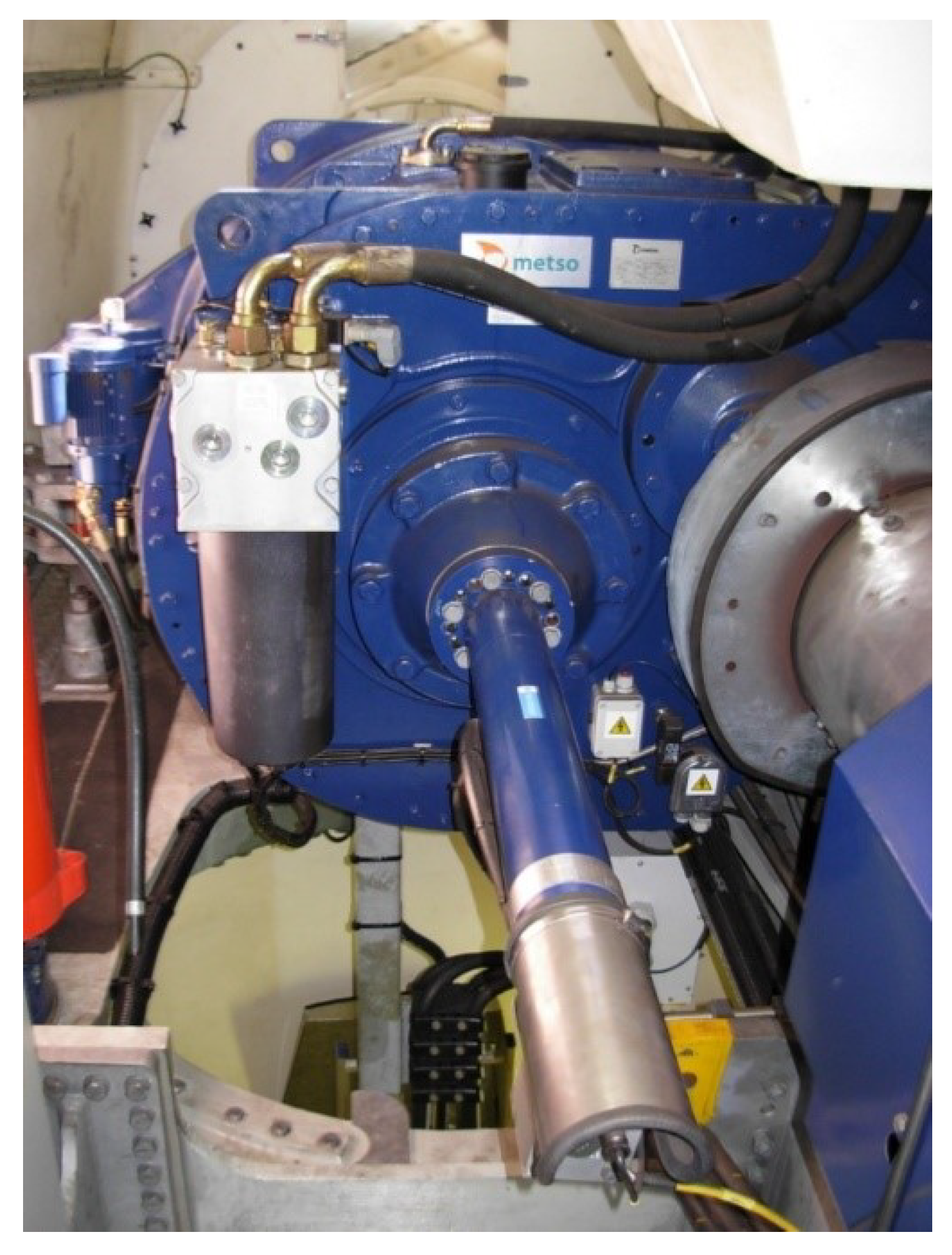
In October 2018, the wind turbine gearbox, shown in Figure 2 and principal specifications in Table 1, reached the end of life, after thirteen years of operation. Based on a gearbox boroscope inspection and oil sample tests, it was recommended by service provider that the gearbox be replaced. Impact marks and indentation on planetary bearing roller were observed along with wear marks on teeth flanks. The oil sample test results showed an elevated copper particle count that was well in excess of the its recommended limit. The gearbox was replaced with brand new gearbox of the same model and specifications in July 2019.
The 10-minute multi-annual SCADA data from the turbine control system is used in this study to examine the impact of gearbox replacement with the aim of assessing gearbox aging on the power and energy performance over the gearbox lifespan. The data used in Table 2 are based on availability and sufficient time apart to examine the aging trends.
3. Methods
The objective of this part of the work is detecting and quantifying the performance degradation of the wind turbine, due to the gearbox aging, through operation data analysis.
In general, it is complex to monitor reliably wind turbine performance because of the multivariate dependence of wind turbine power on ambient conditions and working parameters.
The power of a wind turbine, below its rated speed, is defined as in Equation (1):
where is the air density, A is the area swept by the rotor, is the power factor which is function of the tip speed ratio and of the blade pitch angle . Not only is a non-linear function of and , but the actual power factor can differ from the theoretical one due to environmental effects (like wind shear and turbulence) and due to wind turbine functioning (aging, malfunctioning and so on).
The simplest possible approach for monitoring the power P is to compare the observed power against a benchmark for the power curve, i.e., the relation between the wind speed and the power output. Despite the simplicity of this idea, selecting appropriately a data-driven benchmark power curve is questionable as well, for several reasons:
- Wind turbines are typically equipped with cup anemometers mounted behind the rotor and the undisturbed wind speed is ex-post reconstructed through a nacelle transfer function;
- The power curve has non-trivial seasonal and ambient conditions dependence.
For this reason, therefore, in the wind energy literature, the idea of employing the rotor as wind speed measurement probe has been recently gaining interest: this is the concept of rotor equivalent wind speed [23,24]. Thus, the performance monitoring task can translate into the monitoring of appropriate operation curves (alternative to the power curve), like the rotor speed–power curve [25] and the blade pitch–power curve [25,26].
The idea of this work has been to generalize this concept by formulating a multivariate data-driven model, whose output y is the power of the wind turbine and whose input variables are the most relevant ambient conditions and operation parameters measurements. This kind of approaches has been recently developing in the wind energy literature for performance monitoring and condition monitoring purposes. For some examples, refer to [27,28,29,30]. For a comprehensive point of view about the use of operation data in wind energy and about data-driven power curve models, refer to [31]. In order to test the consistency of the proposed method and to provide as well a more intuitive benchmark, also the binned power curve analysis (as dictated by IEC guidelines [20]) has been adopted (Section 3.3) and the results are qualitatively compared and discussed.
3.1. Support Vector Machine Regression
For the purposes of the present work, a Support Vector Machine Regression with Gaussian kernel has been selected. As a premise, it should be noted that the consistency of this kind of regression for the objectives of the present work has been crosschecked by comparing the results against other kinds of regression, as for example Principal Component Regression (PCR) and Least Absolute Shrinkage and Selection Operator (LASSO) Regression. It arises that the Support Vector Machine Regression outperforms PCR and LASSO regression in terms of mean error, mean absolute error and root mean square error and furthermore the results are more stable from one model run to the other. These have been considered good arguments for considering the Support Vector Machine Regression an adequate method for this study.
The procedure goes as follows: first, let be the matrix of covariates and be the vector of the target (power output). The number of observations is N and we label a generic observation as n-th. Basing on the disposal of operation and ambient data for the present test case, the column vectors of contain the following regressors:
- Undisturbed wind speed average, estimated by the control system through the nacelle transfer function;
- Turbulence intensity, estimated as the ratio between the standard deviation and the average of the undisturbed wind speed;
- Yaw angle;
- Blade pitch angle;
- Rotor speed;
- Generator speed.
The wind speed v has been renormalized () taking into account the external temperature measurement at disposal, as indicated for example in [32] and in the IEC guidelines [33], according to Equations (2) and (3):
with
being the air density in standard conditions (), being the standard temperature 288.15 K and T being the external temperature measured on site in Kelvin units.
In order to understand the principles of Support Vector Regression [34], consider at first a linear model (Equation (4)):
The objective is finding with the minimum norm value subject to the residuals being lower than a threshold for each observation (Equation (14)):
The optimization of the model is basically a trade-off between the flatness of and the amount up to which residuals higher than are tolerated. This can be better formulated in mathematical terms through the Lagrange dual formulation: the function to be minimized is (Equation (6)):
with the constraints (Equation (7))
where C is the box constraint.
The parameters can then be rewritten as indicated in Equation (8):
If either or is different from 0, the corresponding observation is called a support vector.
The model can then be used for predicting new values, given the input observation, through the function (Equation (9)):
A nonlinear Support Vector Regression is obtained by replacing in the above formulas the dot products between observations matrix with a nonlinear Kernel function (Equation (10)):
where is a transformation mapping the observations into a high-dimensional feature space.
A typical selection of the Kernel function has been adopted in this work, i.e., a Gaussian Kernel (Equation (11)):
3.2. The Data Sets Arrangement and the Performance Monitoring
The data sets before gearbox replacement, at disposal to the authors, have been organized in yearly packets:
- ;
- ;
- ;
- ;
- ;
- .
Notice that with the data sets at disposal, it is possible to set the standards for the performance basing on the oldest data set at disposal (2008, when the wind turbine and the gearbox were less than 2 years old) and then it is possible to trace the performance evolution (or, better, degradation) from 2012 up to when the gearbox has been replaced (2018).
The data sets are subsequently employed as follows for the regression:
- is randomly divided in two subsets: D0 (a random selection of of the data set) and D1 (the remainder of the data set). D0 is used for training the regression, D1 is used for testing the regression. The convergence of model training is obtained through the MATLAB® routine.
- A data set posterior to is named as D2 and is used to quantify the performance deviation with respect to 2008.
Once the Support Vector Machine Regression has been trained with the D0 data set, the output is simulated (basing on the input variables observations) for data sets D1 and D2. Since D1 belongs to the baseline data set (i.e., 2008), and D2 is a posterior data set, if the performance of the wind turbine has worsened, it should be possible to quantify this phenomenon by observing how the residuals between measurements Y and simulations vary from D1 to D2. This method has been shown to be effective for performance control and monitoring and has been applied for different, albeit conceptually similar, test cases: the assessment of wind turbine technology optimization, which is expected to result in improved performance [17,18,19,35].
Therefore, consider Equation (14) with .
For , one computes (Equation (15))
and the quantity provides an estimate of the performance deviation from data set D1 to D2.
3.3. Power Curve Analysis
The binning method [36], as dictated by IEC guidelines [20], has been employed for power curve analysis.
Once the wind speed measurements are renormalized according to Equations (2) and (3), power data are grouped in wind speed bins. The typical selection of bin amplitude is 1 or 0.5 m/s, depending on the size of the data set at disposal. For the objectives of the present work, it has been considered appropriate to select 0.5 m/s wind speed bins.
Given the i-th wind speed bin, the average wind speed for the bin is computed as in Equation (16):
and the average power for the bin is computed as in Equation (17):
where is the normalised measured wind speed of the j-th data set in the i-th wind speed bin, is the normalised measured power output of the j-th data set in the i-th wind speed bin and is the population of the i-th wind speed bin.
The power curves have been calculated in this way for the data sets listed in Section 3.2. Having at hand different power curves measured in different periods allows estimating the Annual Energy Production (AEP) trend, if one weights the binned power curves against the same reference wind speed distribution. The data set has been selected as reference for the AEP analysis because it is the data set at disposal corresponding to the lower gearbox and wind turbine aging.
The 2008 reference wind speed distribution is characterised by the well-known Weibull probability function (Equation (18)).
where A is the scale factor and k is the is the shape factor.
This scale and shape factors are determined from the MATLAB® function that is based on the statistical method of moments.
The AEP for a given power curve in the reference wind year can be computed from (Equation (19))
where is the number of hours in a year.
4. Results
4.1. Regression Results
Notice that all the data sets are filtered below rated speed and below rated power, because the performance degradation is not expected to be observable when the operation is at rated power. Therefore, the following results in line of principle should be intended as performance deviation below rated power, with respect to the baseline D0 data set belonging to year 2008. It should be pointed out that the site has a wind distribution predominantly moderate, as is discussed in detail in Section 4.3, and wind intensities above rated occur so rarely that the results for , which are reported in Table 3, can be practically intended as well as AEP average deviations.
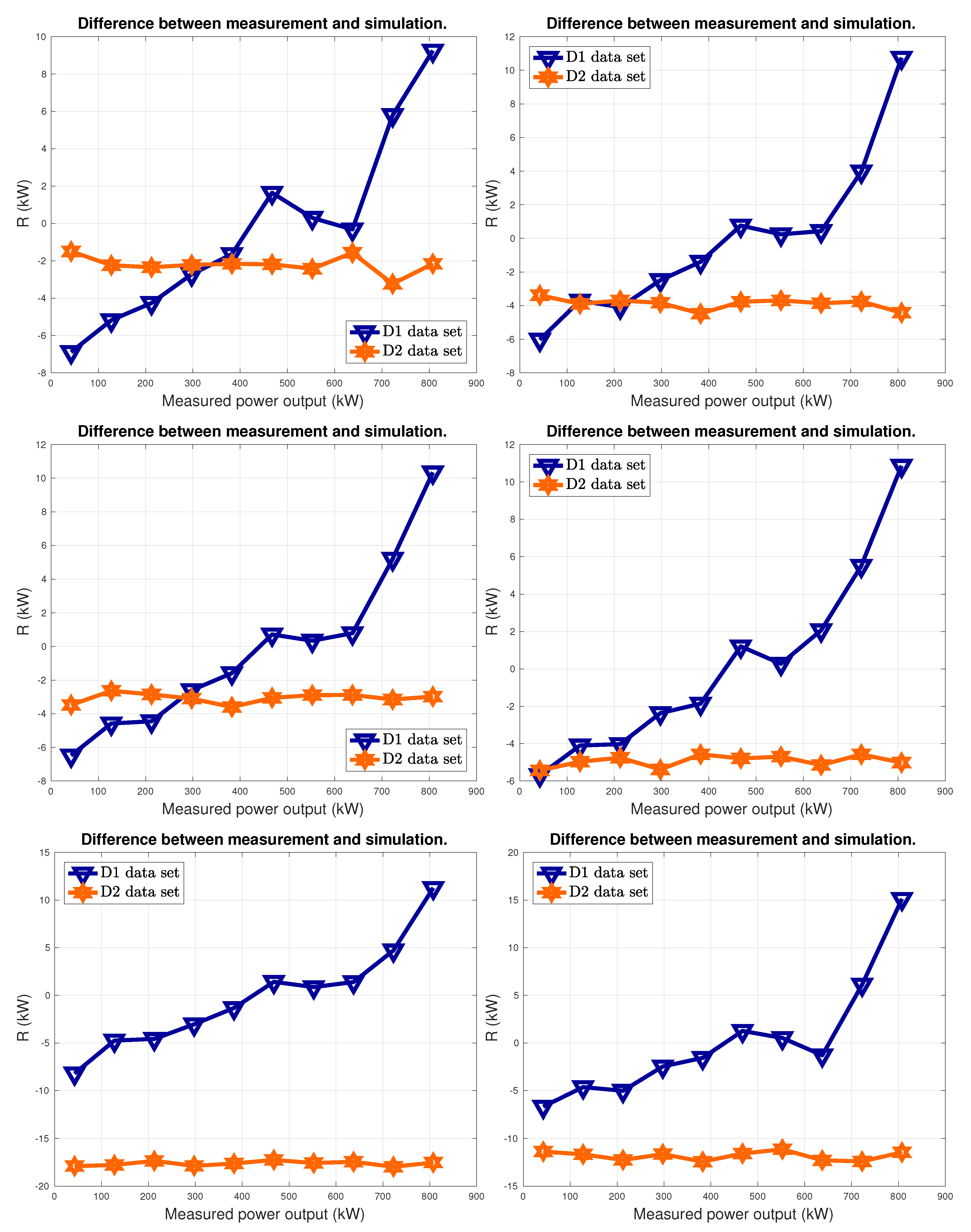
The results in Table 3 can be visualized through the following Figure 3: the sets and (from which the values of in Table 3 have been calculated) are plotted one against the other after being averaged within intervals having amplitude of the 10% of the rated power.
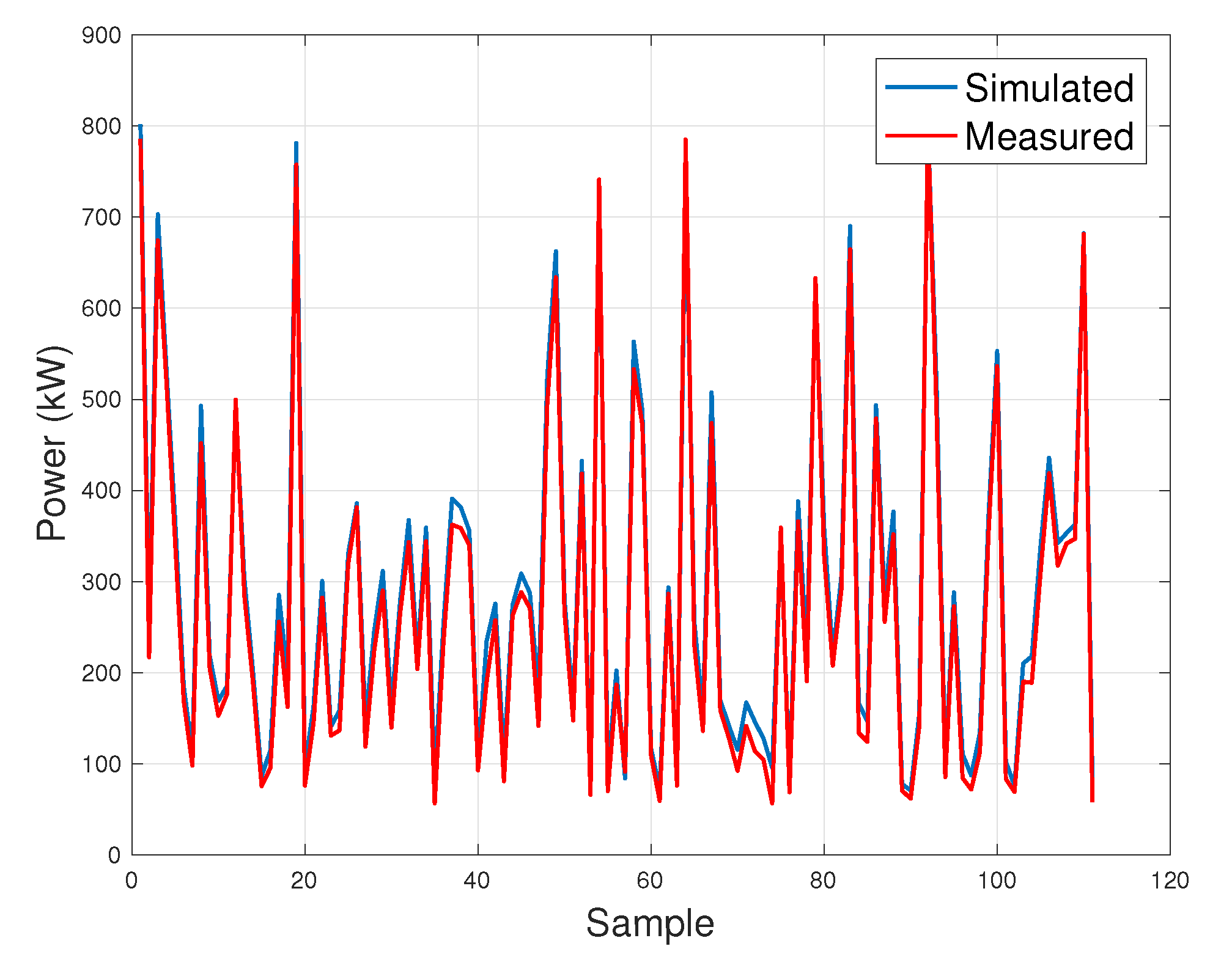
Furthermore, in order to appreciate qualitatively the method, an excerpt of power time series measured during is reported in Figure 4 and is compared against the corresponding simulated time series, when the model is trained with the data. The performance degradation is visible in the fact that the data simulated with the model trained with are slightly higher than the measured data.
It should be noted that the procedure described in Section 3.2 allows producing artificially the replicability of the test, because at each run of the training a different subset D0 (and therefore D1) of is selected. It is appreciable that the results collected in Table 3 are particularly stable: repeating the test several times, one obtains that the standard deviation of the estimates if of the order of .
4.2. Analysis before and after Gearbox Replacement
A data set was at disposal for this study. This data set goes from 28 July 2019 (after the gearbox replacement) to 31 December 2019.
In this regard, it is interesting to compare the data set immediately before the gearbox replacement against the one immediately after the gearbox replacement.
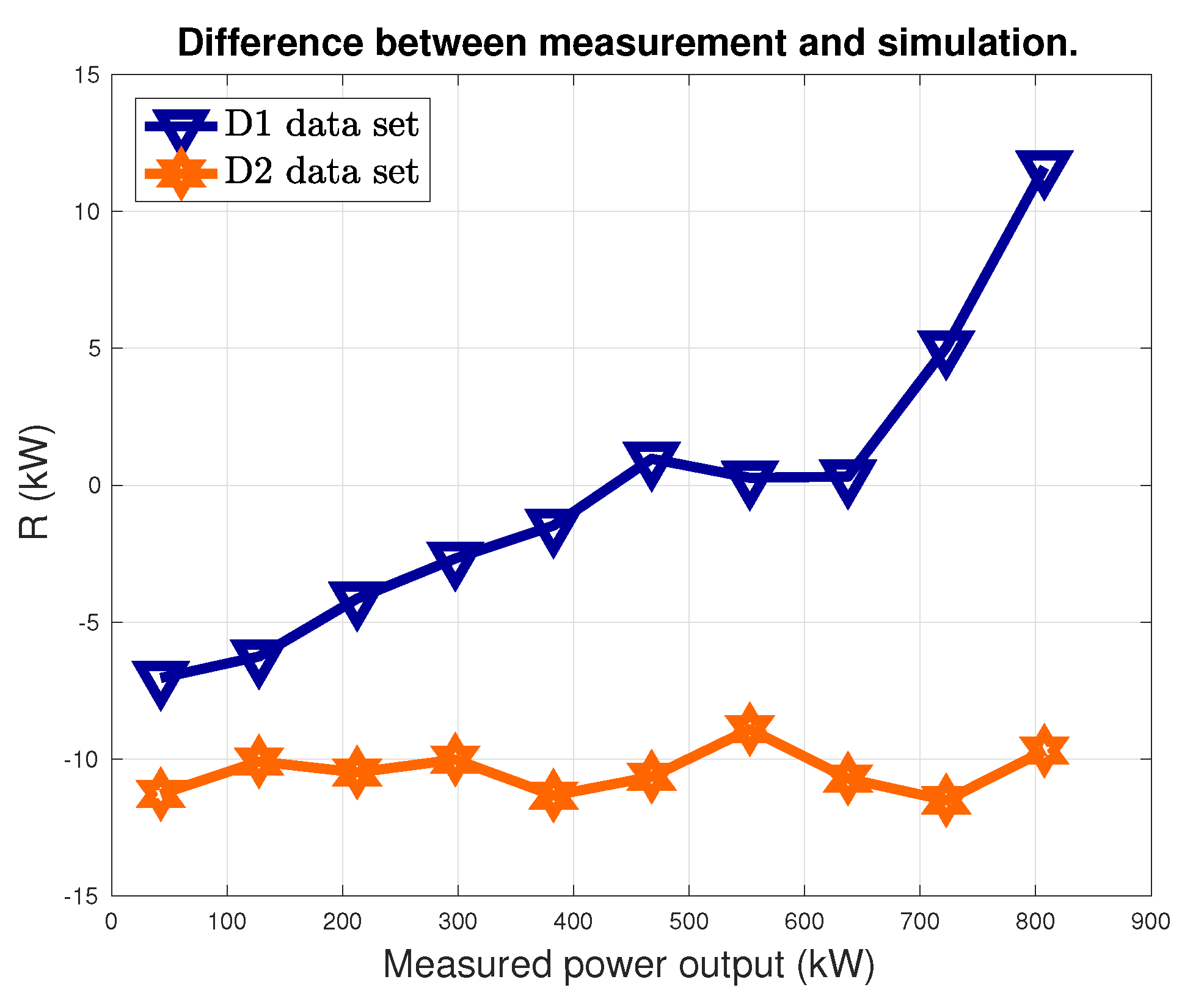
For this reason, the procedure described in Section 3.2 has been applied here on, with D0 and D1 that are extracted (in the same proportions) from data sets and and D2 which coincides with . The result for is reported in Table 4 and in Figure 5 the sets and are plotted one against the other after being averaged within intervals having amplitude of the 10% of the rated power.
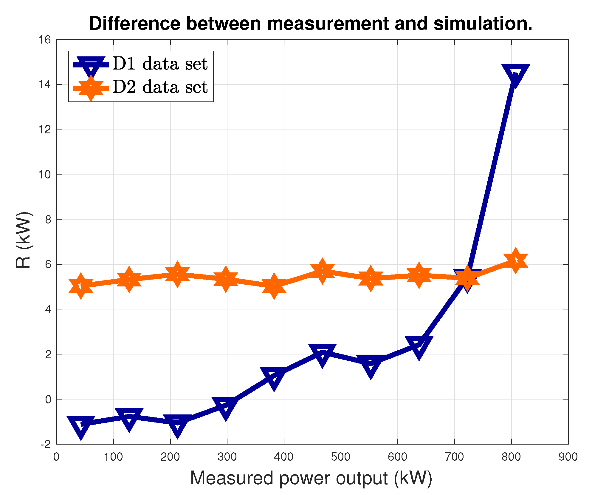
Another interesting analysis is based on the comparison between the reference data set and the data set posterior to the gearbox replacement because it provides an estimate of the impact on performance of the aging of all the wind turbine components except the gearbox (because describes operation with the gearbox). Consider then D0 and D1 selected as in Section 4.1 and D2 coinciding with . The results are collected in Table 5 and Figure 6.
Comparing the results in Table 3 and Table 5, by difference it can be estimated that the gearbox aging weights the order of 40% of the overall performance degradation caused by the aging of all the wind turbine system.
Another interesting aspect is the thermal behavior at the wind turbine gearbox before and after gearbox replacement. The method of [37] has been adopted: in Figure 7, the average curve of the difference between gear oil temperature and external temperature versus power is reported. Data have been averaged in power intervals of the 10% of the rated. Three examples of pre-substitution data sets (2008, 2014, 2017–2018) have been selected and the fourth data set included in the plot is the post-substitution one (2019). From Figure 7, it arises that the data sets before replacement are hardly distinguishable: for readability of the Figure, the standard deviation bars at each point have not been included, but the matter of fact is that the three curves (2008, 2014, 2017–2018) are compatible, while the average gear oil temperature has considerably diminished after gearbox replacement.
4.3. Power Curve Analysis and Production Assessment
The impact on annual energy production (AEP), due variations in the power curves, at different stages over the lifetime of the wind turbine, is assessed for the each of the wind years studied. The AEP using power curves from 2014 and a 12-month period in 2017–2018 are compared to the AEP using the reference power curve from 2008. The AEP comparison is done with each power curve for each wind year. The improvement in AEP from replacing the gearbox in 2019 is examined using the 2019 power curve with the same wind years to investigate the potential contribution of the gearbox alone to energy performance degradation of the wind turbine.
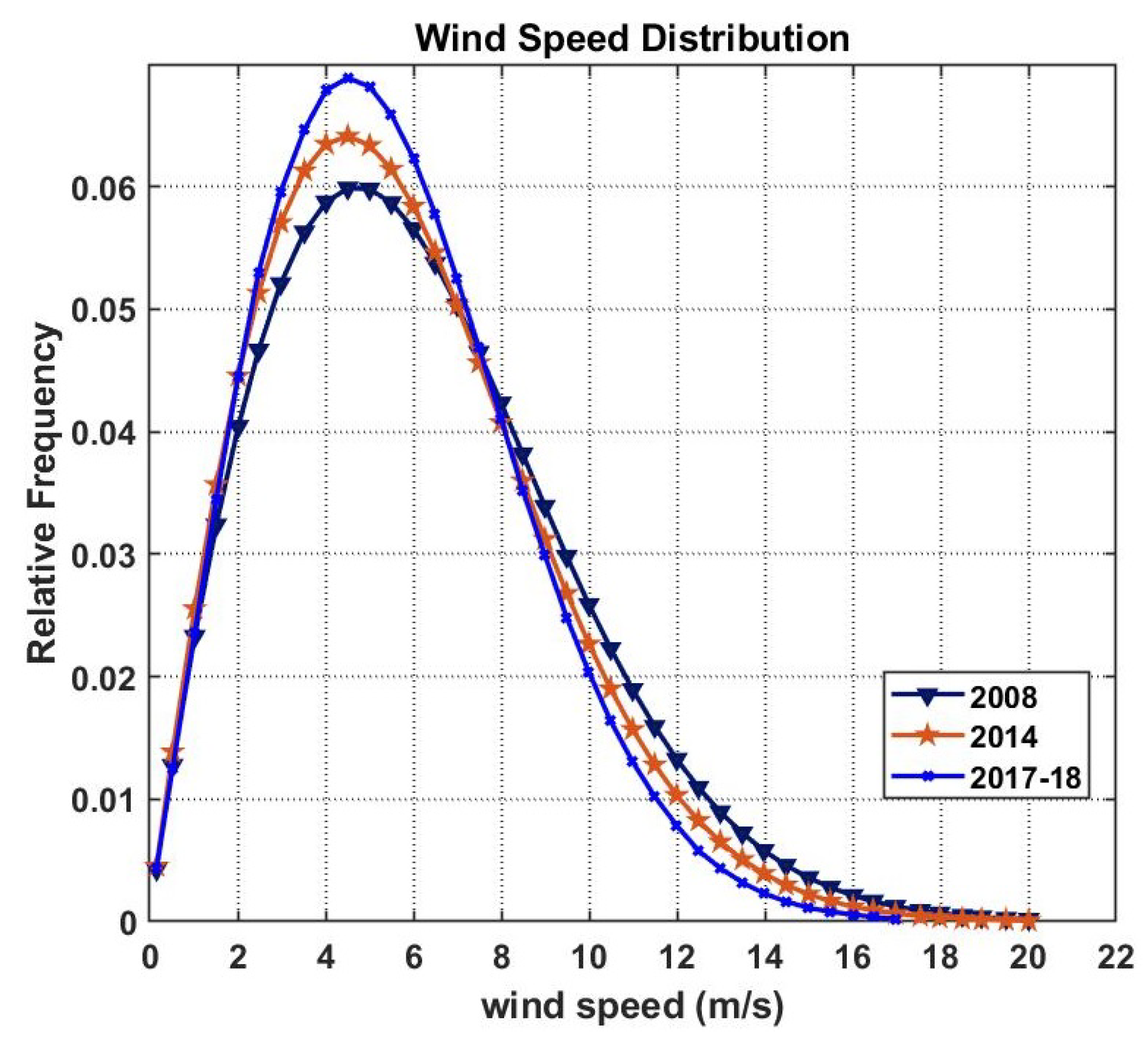
The wind speed distributions of 2008, 2014 and 2017–2018 are shown in Figure 8 and corresponding wind resource parameters are reported in Table 6. It can be seen the site has a relatively low wind resource, with an average annual wind speed of 5.6 m/s to 6.2 m/s. The site would be considered considered an IEC Class IV site.
The power curve of the 2017–2018 period is noticeably different as shown in Figure 9.
The AEP comparison for each power curve in each of the wind years in Table 7 shows, in all cases, a noticeable change in AEP degradation ( AEP) using 2014 and 2017–2018 power curves compared to the 2008 to 2014 power curves (for a detailed discussion about yearly wind energy density analysis, refer to [38]). The AEP degradation is consistently reduced when using the 2019 power curve, which corresponds to the gearbox replacement. The shows that the gearbox replacement in 2019 improves performance, as wound be expected; however, it did not fully return the wind turbine to the 2008 level of performance. For example, taking the the 2008 wind year, the overall 4.3% in AEP degradation using the 2017–2018 power curve is reduced to 3.0% using the 2019 power curve i.e., approximately a 30% contribution to the total AEP degradation from the gearbox alone. Interestingly, this improvement of 30% occurs for the higher wind speed year of 2008 with a lower improvement for the lower wind speed year of 2017–2018, equating to approximately 22%. This suggests that other factors, such as the influence of aging on other components including the blades, pitching system, yaw system, generator and control anemometer are contributors to turbine power degradation. It also suggests that the influence of the gearbox is less significant at lower wind class sites such as in this case.
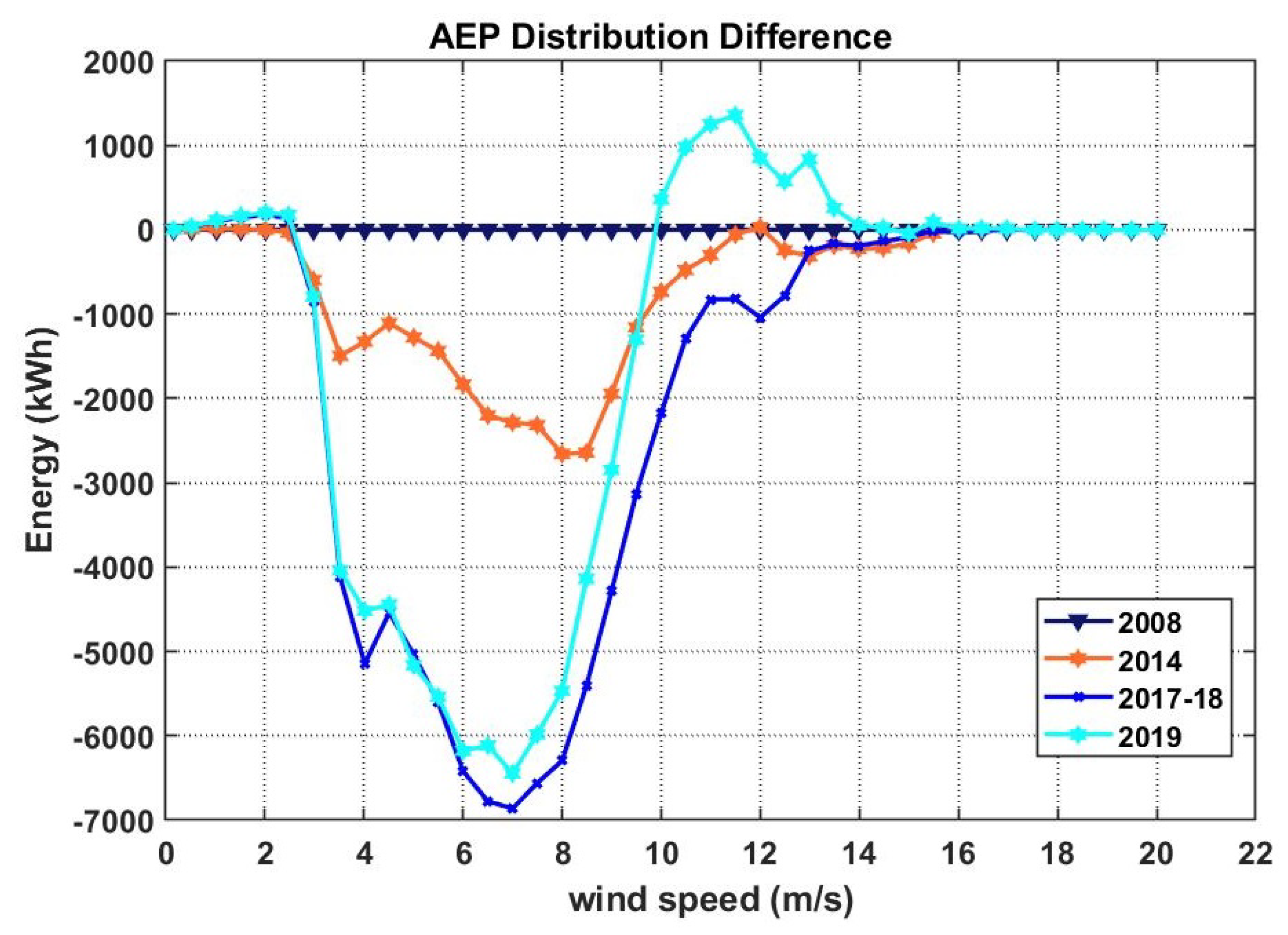
A comparison of the AEP distribution differences with wind speed for each power curve and the 2008 wind year, shown in Figure 10, reveals the degradation can be seen, particularly at wind speeds below rated power where this turbine is operating a large proportion of the time. Also, much of the improvement, due to the gearbox replacement (2019 power curve) occurs, at wind speeds above 6 m/s. This is constant with the better improvement observed in for the the higher wind year of 2008 Table 7. Therefore, similar wind turbines located at wind farms sites with better wind resources can expect to see a better improvement in energy performance with new gearbox replacements compared to turbines at less windy locations.
It is interesting to note that the results in Table 6 are slightly different with respect to Table 3 and Table 4, but the order of magnitude is compatible. This not only is consistent but it is expected, because the methods of Section 3.1 and Section 3.3 are different. The power curve analysis has been based on weighting the measured power curves in different periods against the wind speed distribution of multiple years. This has been done because the only way to estimate the difference in energy production, given two or more measured power curves, is weighting them against a reference distribution. The method in Section 3.1 and Section 3.2 is different because it passes through the analysis of how the residuals between measurements and model estimates change, given certain wind conditions which are input variables to the model. In other words, the method of Section 3.1 and Section 3.2 says that, given and taking into account the wind conditions measured, say, in 2008 and in 2017, the average performance degradation is −6.2% (Table 3). In order to do this, one has to pass through a model and a non-trivial regression task. Summarizing, given the pros and cos of each approach, it is important that they provide consistent results.
In economic terms, as electricity prices can be variable depending on jurisdiction and electricity market prices, a detailed economic study is not the primary focus of this study. However, in this case, a typical average commercial retail electricity unit price is in the region of EUR 0.10 per kWh. This would equate to approximate losses in annual savings of EUR 2700 in 2014 rising to EUR 7800 in the 12 month period during 2017–2018. The gearbox replacement reduces the loss in annual savings back to approximately EUR 5500 i.e., an improvement of EUR 2300.
An indicative total gearbox replacement cost (including crane, all site works etc.), obtained from communications with DkIT, is approximately EUR 70,000 for a refurbished gearbox and EUR 110,000 for a brand new gearbox. These costs do not include any local taxes. A three to six week lead-time for obtaining the gearbox was also indicated. As the biggest power and energy degradation occurred in the final year of the gearbox’s life, the economic loss is relatively small. This shows that, in this case, that is was best to allow the gearbox to run to failure before replacement. It should be noted that the above considerations to not comprehend the more complex framework of condition-based maintenance that is discussed, for example, in [3,31], but can nevertheless be useful indications for wind farm management.
5. Conclusions
This study has been devoted to a data-driven analysis of wind turbine performance decline with age. Operation data from 2008 to 2019 from a Vestas V52 installed at the Dundalk Institute of Technology have been employed. An important added value of the present test case is that the gearbox of the wind turbine reached its end of life in October 2018 and has been substituted: therefore, it has been possible to draw interesting considerations about the aging of the entire system and about the contribution of the gearbox to wind turbine aging and performance degradation.
This study highlights the potential value of machine learning, in particular Support Vector Regression with Gaussian Kernel, in analysing SCADA data on an ongoing bases to monitor wind turbine performance degradation. This can improve logistical and financial planning for large component replacements, thereby minimising wind turbine down-times at times of large component replacements. Separate approaches to power and energy degradation analysis, in this case, draw similar conclusions. Specifically, an overall wind turbine power and energy degradation in the order of 5% has been determined over the 13-year lifetime of the wind turbine, with the gearbox contributing approximately a 30% share to the degradation. These two main results have been shown not to depend remarkably on the energy density contained in the reference data set. Replacing the gearbox shows best improvement in energy output above wind speeds of 6 m/s suggesting that the gearbox aging has a smaller influence at lower wind class sites. Allowing the gearbox to run to failure is indicated to be economically justified, showing that the gearbox has been quite robust and not the dominant factor in performance degradation. Finally, the results of the present work about wind turbine aging are more in line with those in [12] than in [14]: actually, if one extrapolates the present results to a twenty years period, the estimate agrees with [12]. It should be noted that, differently with respect to what observed in [12], the results of this study do not conform well to the hypothesis that the aging degradation is linear in time: actually, up to 7 years after the reference data set, the performance worsening is estimated to be of the order of 1%, while 10 years later the worsening reaches the 5%.
The findings add to the broader debate on whether direct-drive gearless wind turbine technology is a significantly better option compared with gear based technology. This may have broader implications for ever increasing number of older wind turbines and wind farms around the world are nearing the end of operational life in the context of turbine re-powering options. Further research in these techniques, using operational data from a broader range of sites and turbine technologies to improve decision making processes in the operation and re-powering of wind farms, would be of great benefit to the industry.
Author Contributions
Conceptualization, D.A., R.B., N.J.H. and F.C.; Data curation, D.A., R.B. and N.J.H.; Formal analysis, D.A., R.B. and F.C.; Investigation, D.A., R.B. and F.C.; Methodology, D.A. and R.B.; Project administration, R.B. and F.C.; Software, D.A.; Supervision, R.B. and F.C., Validation, D.A., R.B. and F.C.; Writing—original draft, D.A. and R.B.; Writing—review & editing, D.A., R.B., N.J.H. and F.C. All authors have read and agreed to the published version of the manuscript.
Acknowledgments
The authors acknowledge Fondazione “Cassa di Risparmio di Perugia” for the funded research project WIND4EV (WIND turbine technology EVolution FOR lifecycle optimization). The authors also wish to acknowledge the support of the INTERREG VA SPIRE2 project. This research was supported by the European Union’s INTERREG VA Programme (Grant No. INT-VA/049), managed by the Special EU Programmes Body (SEUPB). The views and opinions expressed in this document do not necessarily reflect those of the European Commission or the Special EU Programmes Body (SEUPB).
Conflicts of Interest
The authors declare no conflict of interest.
References
- Kumar, Y.; Ringenberg, J.; Depuru, S.S.; Devabhaktuni, V.K.; Lee, J.W.; Nikolaidis, E.; Andersen, B.; Afjeh, A. Wind energy: Trends and enabling technologies. Renew. Sustain. Energy Rev. 2016, 53, 209–224. [Google Scholar] [CrossRef]
- He, D.; Li, Y. Overview of Worldwide Wind Power Industry. In Strategies of Sustainable Development in China’s Wind Power Industry; Springer: Singapore, 2020; pp. 29–60. [Google Scholar]
- Byon, E.; Ntaimo, L.; Singh, C.; Ding, Y. Wind energy facility reliability and maintenance. In Handbook of Wind Power Systems; Springer: Berlin/Heidelberg, Germany, 2013; pp. 639–672. [Google Scholar]
- Artigao, E.; Martín-Martínez, S.; Honrubia-Escribano, A.; Gómez-Lázaro, E. Wind turbine reliability: A comprehensive review towards effective condition monitoring development. Appl. Energy 2018, 228, 1569–1583. [Google Scholar] [CrossRef]
- Echavarria, E.; Hahn, B.; Van Bussel, G.; Tomiyama, T. Reliability of wind turbine technology through time. J. Sol. Energy Eng. 2008, 130. [Google Scholar] [CrossRef]
- Carroll, J.; McDonald, A.; McMillan, D. Failure rate, repair time and unscheduled O&M cost analysis of offshore wind turbines. Wind Energy 2016, 19, 1107–1119. [Google Scholar]
- Yang, W.; Court, R.; Jiang, J. Wind turbine condition monitoring by the approach of SCADA data analysis. Renew. Energy 2013, 53, 365–376. [Google Scholar] [CrossRef]
- Zaher, A.; McArthur, S.; Infield, D.; Patel, Y. Online wind turbine fault detection through automated SCADA data analysis. Wind Energy Int. J. Prog. Appl. Wind Power Convers. Technol. 2009, 12, 574–593. [Google Scholar] [CrossRef]
- Butler, S.; Ringwood, J.; O’Connor, F. Exploiting SCADA system data for wind turbine performance monitoring. In Proceedings of the 2013 IEEE Conference on Control and Fault-Tolerant Systems (SysTol), Nice, France, 9–11 October 2013; pp. 389–394. [Google Scholar]
- Lapira, E.; Brisset, D.; Ardakani, H.D.; Siegel, D.; Lee, J. Wind turbine performance assessment using multi-regime modeling approach. Renew. Energy 2012, 45, 86–95. [Google Scholar] [CrossRef]
- Long, H.; Wang, L.; Zhang, Z.; Song, Z.; Xu, J. Data-driven wind turbine power generation performance monitoring. IEEE Trans. Ind. Electron. 2015, 62, 6627–6635. [Google Scholar] [CrossRef]
- Staffell, I.; Green, R. How does wind farm performance decline with age? Renew. Energy 2014, 66, 775–786. [Google Scholar] [CrossRef] [Green Version]
- Kurz, R.; Brun, K. Degradation of gas turbine performance in natural gas service. J. Nat. Gas Sci. Eng. 2009, 1, 95–102. [Google Scholar] [CrossRef]
- Olauson, J.; Edström, P.; Rydén, J. Wind turbine performance decline in Sweden. Wind Energy 2017, 20, 2049–2053. [Google Scholar] [CrossRef]
- Dai, J.; Yang, W.; Cao, J.; Liu, D.; Long, X. Ageing assessment of a wind turbine over time by interpreting wind farm SCADA data. Renew. Energy 2018, 116, 199–208. [Google Scholar] [CrossRef] [Green Version]
- Smola, A.J.; Schölkopf, B. A tutorial on support vector regression. Stat. Comput. 2004, 14, 199–222. [Google Scholar] [CrossRef] [Green Version]
- Lee, G.; Ding, Y.; Xie, L.; Genton, M.G. A kernel plus method for quantifying wind turbine performance upgrades. Wind Energy 2015, 18, 1207–1219. [Google Scholar] [CrossRef]
- Hwangbo, H.; Ding, Y.; Eisele, O.; Weinzierl, G.; Lang, U.; Pechlivanoglou, G. Quantifying the effect of vortex generator installation on wind power production: An academia-industry case study. Renew. Energy 2017, 113, 1589–1597. [Google Scholar] [CrossRef]
- Astolfi, D.; Castellani, F.; Terzi, L. Wind Turbine Power Curve Upgrades. Energies 2018, 11, 1300. [Google Scholar] [CrossRef] [Green Version]
- International Electrotechnical Commission. Wind Energy Generation Systems—Part 12-1: Power Performance Measurements of Electricity Producing Wind Turbines; Technical Report, IEC 61400-12-1: 2017; International Electrotechnical Commission: Geneva, Switzerland, 2007. [Google Scholar]
- Sequeira, C.; Pacheco, A.; Galego, P.; Gorbeña, E. Analysis of the efficiency of wind turbine gearboxes using the temperature variable. Renew. Energy 2019, 135, 465–472. [Google Scholar] [CrossRef]
- Byrne, R.; Hewitt, N.J.; Griffiths, P.; MacArtain, P. Observed site obstacle impacts on the energy performance of a large scale urban wind turbine using an electrical energy rose. Energy Sustain. Dev. 2018, 43, 23–37. [Google Scholar] [CrossRef]
- Choukulkar, A.; Pichugina, Y.; Clack, C.T.; Calhoun, R.; Banta, R.; Brewer, A.; Hardesty, M. A new formulation for rotor equivalent wind speed for wind resource assessment and wind power forecasting. Wind Energy 2016, 19, 1439–1452. [Google Scholar] [CrossRef]
- Scheurich, F.; Enevoldsen, P.B.; Paulsen, H.N.; Dickow, K.K.; Fiedel, M.; Loeven, A.; Antoniou, I. Improving the accuracy of wind turbine power curve validation by the rotor equivalent wind speed concept. J. Phys. Conf. Ser. IOP Publ. 2016, 753, 072029. [Google Scholar] [CrossRef] [Green Version]
- Pandit, R.; Infield, D. Comparative analysis of binning and support vector regression for wind turbine rotor speed based power curve use in condition monitoring. In Proceedings of the IEEE 2018 53rd International Universities Power Engineering Conference (UPEC), Glasgow, UK, 4–7 September 2018; pp. 1–6. [Google Scholar]
- Pandit, R.K.; Infield, D. Comparative assessments of binned and support vector regression-based blade pitch curve of a wind turbine for the purpose of condition monitoring. Int. J. Energy Environ. Eng. 2019, 10, 181–188. [Google Scholar] [CrossRef] [Green Version]
- Marvuglia, A.; Messineo, A. Monitoring of wind farms’ power curves using machine learning techniques. Appl. Energy 2012, 98, 574–583. [Google Scholar] [CrossRef]
- Kusiak, A.; Verma, A. Monitoring wind farms with performance curves. IEEE Trans. Sustain. Energy 2012, 4, 192–199. [Google Scholar] [CrossRef]
- Song, Z.; Zhang, Z.; Jiang, Y.; Zhu, J. Wind turbine health state monitoring based on a Bayesian data-driven approach. Renew. Energy 2018, 125, 172–181. [Google Scholar] [CrossRef]
- Zhang, J.; Jiang, N.; Li, H.; Li, N. Online health assessment of wind turbine based on operational condition recognition. Trans. Inst. Meas. Control 2019, 41, 2970–2981. [Google Scholar] [CrossRef]
- Ding, Y. Data Science for Wind Energy; CRC Press: Boca Raton, FL, USA, 2019. [Google Scholar]
- Astolfi, D.; Castellani, F.; Garinei, A.; Terzi, L. Data mining techniques for performance analysis of onshore wind farms. Appl. Energy 2015, 148, 220–233. [Google Scholar] [CrossRef]
- International Electrotechnical Commission. Power Performance Measurements of Electricity Producing Wind Turbines; Technical Report 61400-12; International Electrotechnical Commission: Geneva, Switzerland, 2005. [Google Scholar]
- Vapnik, V. The Nature of Statistical Learning Theory; Springer Science & Business Media: Berlin/Heidelberg, Germany, 2013. [Google Scholar]
- Astolfi, D.; Castellani, F. Wind turbine power curve upgrades: Part II. Energies 2019, 12, 1503. [Google Scholar] [CrossRef] [Green Version]
- Pandit, R.K.; Infield, D. Comparison of binned and Gaussian Process based wind turbine power curves for condition monitoring purposes. J. Maint. Eng. 2018, 2. [Google Scholar]
- Astolfi, D.; Castellani, F.; Terzi, L. Fault prevention and diagnosis through scada temperature data analysis of an onshore wind farm. Diagnostyka 2014, 15. [Google Scholar]
- Tomporowski, A.; Flizikowski, J.; Kasner, R.; Kruszelnicka, W. Environmental control of wind power technology. Rocz. Ochr. Srodowiska 2017, 19, 694–714. [Google Scholar]
Figure 1.
Vestas V52 wind turbine at DkIT.

Figure 2.
Metso PLH-400V52 gearbox.

Figure 3.
The average difference R between power measurement Y and estimation (Equation (14)). Data sets, respectively: 2008 vs. 2012, 2013, 2014, 2015, 2017, 2018.
Figure 3.
The average difference R between power measurement Y and estimation (Equation (14)). Data sets, respectively: 2008 vs. 2012, 2013, 2014, 2015, 2017, 2018.

Figure 4.
Simulated and measured power time series sample: .

Figure 5.
The average difference R between power measurement Y and estimation (Equation (14)). Data sets: 2017–2018 and 2019.
Figure 5.
The average difference R between power measurement Y and estimation (Equation (14)). Data sets: 2017–2018 and 2019.

Figure 6.
The average difference R between power measurement Y and estimation (Equation (14)). Data sets: 2008 and 2019.
Figure 6.
The average difference R between power measurement Y and estimation (Equation (14)). Data sets: 2008 and 2019.

Figure 7.
The power–gear oil temperature curve. Data sets 2008, 2014, 2017–2018 and 2019.

Figure 8.
Annual wind speed distributions.

Figure 9.
Power curves—2008, 2014, 2017–2018 and 2019.

Figure 10.
AEP variations compared to 2008 reference year.


Table 1.
Gearbox -principal specifications.
| Specification | Data |
|---|---|
| Model | PLH-400V52 |
| Rated Power | 935 kW |
| Rated RPM (Low speed shaft) | 26 min |
| Gearing ratio | 61.799 |
| Weight | 5400 kg |
Table 2.
SCADA parameters analysed.
| Parameter | Logging Interval | Years Available |
|---|---|---|
| Wind Speed (m/s) | 10 min. | 2008, 2014, 2017–2018 (12 months), 2019 (6 months) |
| Wind Speed Standard Deviation (m/s) | 10 min. | 2008, 2014, 2017–2018 (12 months), 2019 (6 months) |
| Wind Direction (deg) | 10 min. | 2008, 2014, 2017–2018 (12 months), 2019 (6 months) |
| Ambient Temperature (°C) | 10 min. | 2008, 2014, 2017–2018 (12 months), 2019 (6 months) |
| Rotor Speed (RPM) | 10 min. | 2008, 2014, 2017–2018 (12 months), 2019 (6 months) |
| Blade Pitch Angle (deg) | 10 min. | 2008, 2014, 2017–2018 (12 months), 2019 (6 months) |
| Generator Speed (RPM) | 10 min. | 2008, 2014, 2017–2018 (12 months), 2019 (6 months) |
| Power (kW) | 10 min. | 2008, 2014, 2017–2018 (12 months), 2019 (6 months) |
| Gear oil Temperature (°C) | 10 min. | 2008, 2014, 2017–2018 (12 months), 2019 (6 months) |
Table 3.
Estimate of the production degradation with aging (below rated power).
| Data Set | |
|---|---|
| 2012 vs. 2008 | −0.1% |
| 2013 vs. 2008 | −0.7% |
| 2014 vs. 2008 | −0.4% |
| 2015 vs. 2008 | −1.1% |
| 2017 vs. 2008 | −6.2% |
| 2018 vs. 2008 | −4.0% |
Table 4.
Estimate of the performance change before and after gearbox replacement. (below rated power).
Table 4.
Estimate of the performance change before and after gearbox replacement. (below rated power).
| Data Set | |
|---|---|
| 2019 vs. 2017–2018 | +1.9% |
Table 5.
Estimate of the performance change: 2008 vs. 2019 after gearbox replacement. (below rated power).
Table 5.
Estimate of the performance change: 2008 vs. 2019 after gearbox replacement. (below rated power).
| Data Set | |
|---|---|
| 2008 vs. 2019 | −2.9% |
Table 6.
Annual wind resource and power density parameters.
| Year | Uave (m/s) | Weibull A (m/s) | Weibull k | Power Density (W/m) |
|---|---|---|---|---|
| 2008 | 6.2 | 6.95 | 1.91 | 280.5 |
| 2014 | 5.8 | 6.54 | 1.93 | 227.2 |
| 2017–2018 | 5.6 | 6.32 | 2.04 | 196.6 |
Table 7.
Comparisons of AEP variation with power curve and gearbox replacement.
| Wind Year | Power Curve | AEP (kWh) | AEP (kWh) | % AEP |
|---|---|---|---|---|
| 2008 | 2008 | 1,837,900 | - | - |
| 2014 | 1,810,700 | −27,200 | −1.5% | |
| 2017–2018 | 1,759,600 | −78,300 | −4.3% | |
| 2019 | 1,782,200 | −55,700 | −3.0% | |
| 2014 | 2008 | 1,598,300 | - | - |
| 2014 | 1,571,500 | −26,800 | −1.7% | |
| 2017–2018 | 1,520,200 | −78,100 | −4.9% | |
| 2019 | 1,539,900 | −58,400 | −3.6% | |
| 2017–2018 (12 months) | 2008 | 1,434,500 | - | - |
| 2014 | 1,407,300 | −27,200 | −1.9% | |
| 2017–2018 | 1,354,400 | −80,100 | −5.6% | |
| 2019 | 1,372,000 | −62,500 | −4.4% |
© 2020 by the authors. Licensee MDPI, Basel, Switzerland. This article is an open access article distributed under the terms and conditions of the Creative Commons Attribution (CC BY) license (http://creativecommons.org/licenses/by/4.0/).
Share and Cite
MDPI and ACS Style
Byrne, R.; Astolfi, D.; Castellani, F.; Hewitt, N.J. A Study of Wind Turbine Performance Decline with Age through Operation Data Analysis. Energies 2020, 13, 2086. https://doi.org/10.3390/en13082086
AMA Style
Byrne R, Astolfi D, Castellani F, Hewitt NJ. A Study of Wind Turbine Performance Decline with Age through Operation Data Analysis. Energies. 2020; 13(8):2086. https://doi.org/10.3390/en13082086
Chicago/Turabian StyleByrne, Raymond, Davide Astolfi, Francesco Castellani, and Neil J. Hewitt. 2020. "A Study of Wind Turbine Performance Decline with Age through Operation Data Analysis" Energies 13, no. 8: 2086. https://doi.org/10.3390/en13082086
Note that from the first issue of 2016, this journal uses article numbers instead of page numbers. See further details here.