Low-Capacity Exploitation of Distribution Networks and Its Effect on the Planning of Distribution Networks


1
Department of Electric Engineering, Universidad Distrital Francisco José de Caldas, Bogotá 111321, Colombia
2
Department of Electric and Electronic Engineering, Universidad Nacional de Colombia, Bogotá 111321, Colombia
3
Advanced Power and Energy Center, Electrical Engineering and Computer Science, Khalifa University, Abu Dhabi 127788, UAE
*
Author to whom correspondence should be addressed.
Energies 2020, 13(8), 1920; https://doi.org/10.3390/en13081920
Submission received: 15 March 2020
/
Revised: 10 April 2020
/
Accepted: 13 April 2020
/
Published: 14 April 2020
(This article belongs to the Special Issue Electric Distribution System Modeling and Analysis)
Abstract
:The continuous variation and dispersion of the load demand during a 24-h day are uncontrolled aspects that affect the efficiency, operational conditions, and total cost of the power distribution network. The cost of the network is strongly related to the peak of demand, but the available capacity of the network is not used efficiently during the day because feeders and branches usually work under 70% of their full capacity. In this way, it is necessary to measure how efficiently the distribution network capacity is used and to identify the aspects that can be modified to improve it. This article proposes a new exploitation capacity index to measure the efficiency of a/the whole distribution network throughout the day in relation to the total available capacity of the branches that compose the network. The paper presents the mathematical formulation and the validation process of the index, and then it provides a planning case study in which the index and the total cost of the planning problem are calculated and compared in four different scenarios in which the peak of the load demand changes. The results show a direct relation between the exploitation capacity and the peak of demand, so lower exploitation capacities are strongly related to higher peaks of demand. As for the capital investments for the network planning, it is found that higher peaks of demand involve more upgrade necessities and higher capital investments compared to the other cases.

1. Introduction
Efficiency is one of the aspects that must be improved when designing a project or a network because it is directly related to the technical feasibility and the financial viability of the project. It is not easy to achieve good efficiency levels when working the distribution network (DN) because of the low utilization levels of the feeder’s capacity. This occurs because the continuous variation in the power demand makes the network use a high capacity of the feeders during periods of peak demand or low capacity of feeders during periods of low demand [1]. Such behavior is due to the variable demand and outcome of consumers’ habits in power consumption, which is difficult to control due to its random nature [2]. However, it has a high impact on the design of power distribution networks, estimation of energy losses, and identification of the required capital investment.
The continuous growth of annual demand involves the expansion and upgrade of power distribution networks to ensure that the demand is met. Estimating the peak demand is mandatory, a criterion in network design, as it affects any decision on upgrades and identification of the capital requirement.
The design of power distribution networks involves meeting the technical requirements, such as defining the substation capacity and control of losses and managing both the reactive power and voltage drops [3,4,5]. In addition to the technical aspects, design and planning should include other criteria like the operational lifetime, the reserve capacity, and the reliability of the network [6,7].
The energy distribution system could be reviewed as an imperfect dynamical system. In fact, in spite of the uncertainty of the plant that characterizes it, the modeling of this kind of system can add value to identify and to control the network. The imperfect systems are a good topic to discover these aspects [8]. Additionally, the management and upgrade of power distribution networks are increasingly difficult processes because of the new energy requirements caused by the integration of new technologies, such as electric vehicles [9,10], which have changed the way energy consumption and markets have operated over the last years.
The new EV loads and their characteristic dispersed allocation on different parts of the DN will affect the whole power distribution network and will consequently demand an increased power capacity and capital investment not previously required if an adequate energy management strategy is not implemented [11]. Furthermore, networks will need better management strategies to increase the efficiency and used capacity of an asset as a possible solution to improve the operational conditions on DN and to reduce the DN capital necessities.
The efficient use of DNs currently becomes an important aspect to improve when the daily operation and the planning of DNs because of the limited capital investments available for the upgrade and expansion of the network. This approach can be found in [12], which proposes a methodology to prioritize the places in which investments are more necessary to ensure the supply of energy based on the operational efficiency of the DN. It proposes two indices: Factor X and factor Q. Investments and efficiency are also analyzed in [13], which examines the relation between investment ad energy efficiency on the Croatian DN, based on the demand growth between different areas of the DN as a strategy to optimize the capital invested in the respective areas as a way to reduce energy losses and the capital investments.
Some researchers have focused their works on energy savings and loss reduction as a way to improve the DN efficiency: For example, in [14], different strategies to reduce DN energy losses in Sarawak, Malaysia were analyzed. The authors in [15,16] and [17] proposed to improve the DN efficiency through the feeder’s reconfiguration. This technique improves DN’s operational conditions and reduces energy losses. In [18] and [19], strategies are proposed to manage the energy losses by controlling the bus voltages through a Vol-VAR (reactive power) control.
Another approach frequently used to reduce energy losses and to improve the DN efficiency is distributed generation (DG). Some researchers, such as those in [20] and [21], have employed network reconfiguration and integration of DG units to improve the efficiency of energy use, focused on losses reduction. In the case of [22], PV-distributed generation was used to improve the energy efficiency and power quality simultaneously, while in [23], the DG hosting capacity was maximized based on RES (Renewable Energy Sources) resources, to obtain a deal between private investors and distribution network operators (DNOs), focused on energy efficiency.
A third approach to improve energy efficiency is to increase the loadability in transformers and feeders. It can be performed through DG integration, network reconfiguration, and the use of reactive power compensators to control and manage the DN operational conditions while increasing the loadability on feeders and transformers. As a result of implementing management strategies, it is possible to reduce overload conditions, power losses, and the feeder’s congestion as described in [24,25,26]. The author in [27] used a management strategy to maximize the feeder’s loadability and to minimize the total energy losses simultaneously.
Another common way to improve the network efficiency is to increase the assets’ capacity utilization. This makes it possible to extend the lifetime of assets and also defer the investment necessities because it reaches a more efficient use of the asset during the DN operation.
The capacity utilization is an index used to calculate how the available capacity of assets is used in a specific time during their working time. This index is frequently used to determine if transformers work around an efficient working point and if there is an overload risk condition that could reduce the reliability of the transformer.
The authors in [28] proposed a method to calculate and rank the feeders’ capacity for the implementation of DER, which was calculated based on the peak load with DER and the expected peak load without DER. In [29], a model was proposed to calculate the overall efficiency of DN, including the energy efficiency, asset efficiency, and human resources efficiency, but in this case, a mathematical model to calculate the feeders’ usability was also proposed; it aimed to determine how efficiently the DN is used. This index is calculated based on the peak load, load factor, installed capacity, and operational time of the DN. In [30], the asset utilization rate is part of the indices to calculate the rate cycle life of assets on the DNs.
The capacity utilization is also calculated to know the feeder’s loadability on DN. Most of the works calculate the capacity utilization in a specific feeder or branch, in a specific time (usually the peak time), and then calculate the available capacity of the feeder during the peak demand time. In [31], a method was proposed to calculate the efficiency in the use of the assets on the DN through a methodology that includes the equipment’s and network’s efficiency indices, based on the implementation of a hierarchy strategy that ponders the importance of assets during the DN working time. The methodology proposes a way to calculate the equipment operation efficiency based on the LDC and the used capacity during the assets’ working time. In other cases, equipment utilization indices as the capacity factor, the equipment efficiency rating, and the life cycle utilization of assets have been used to improve the capacity utilization of feeders and assets when including photovoltaic (PV) distributed generation [32].
After reviewing related research studies, no works proposing a method or index to calculate either the timely usability of the feeders or the relevance of every branch on the whole DN were found. Therefore, no indices have been designed to calculate the exploitation capacity of the network nor indices to calculate how efficiently each of the DN branches is used, or how the network capacity is used to schedule the whole day. Information about the overall efficiency of the network and feeders makes it possible to identify those buses that are relevant to more greatly impact on the network efficiency and the implementation of strategies to improve the overall efficiency of the network. By using such information, it might be possible to obtain additional benefits, such as the reduction of losses and the reduction of capital investment necessities.
This work proposes a new index to calculate the exploitation capacity of the network based on the capacity of feeders, which is truly used during the daily operation of the network. In addition, a method to calculate the efficiency when using each feeder of the power distribution network is also proposed. The second part of the article analyzes the effect of the exploitation capacity and its impact on the technical and financial requirements during the planning of power distribution networks by calculating power losses, voltage variation, and total cost of the planning.
This paper presents new indices to calculate the efficiency and the exploitation capacity of the DN, which can be used to know how efficiently the available capacity of the feeders is used within a day, taking into account the available capacity of the DN and the hourly demand of power. Section 1 explains why an efficient use of assets helps improve the operational and financial process in an industrial company and how this concept could influence the operational and financial feasibility of a power distribution network. Section 2 shows the relevance of the power demand in the design and planning of the DN based on the load demand profile. Section 3 presents the mathematical formulation and the validation process of the proposed indices. The last section examines the correlation between the indices values and the technical and financial planning requirements of the DN, and identifies that low index values reveal low efficiency in using the available capacity of the network, but they are also correlated with higher upgrading and financial requirements as compared with cases that show higher index values.
2. Distribution Planning Problem Statement
2.1. Load Duration Curve and its Characteristic Behavior
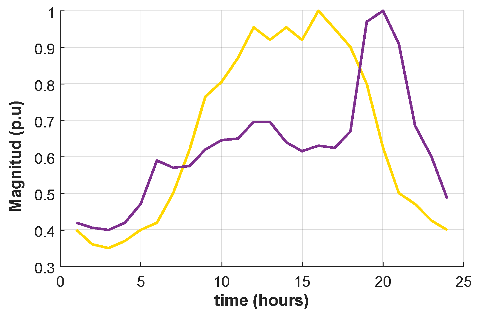
The demand profile is a pattern of demand consumption that represents how users demand power on an hourly basis within a day (as shown in Figure 1).
This kind of profile is used to identify the pattern of energy consumption of a type of customer, to estimate the daily energy consumption, and to determine the peak demand of the users in the measurement point of the DN, among other important aspects described in [30].
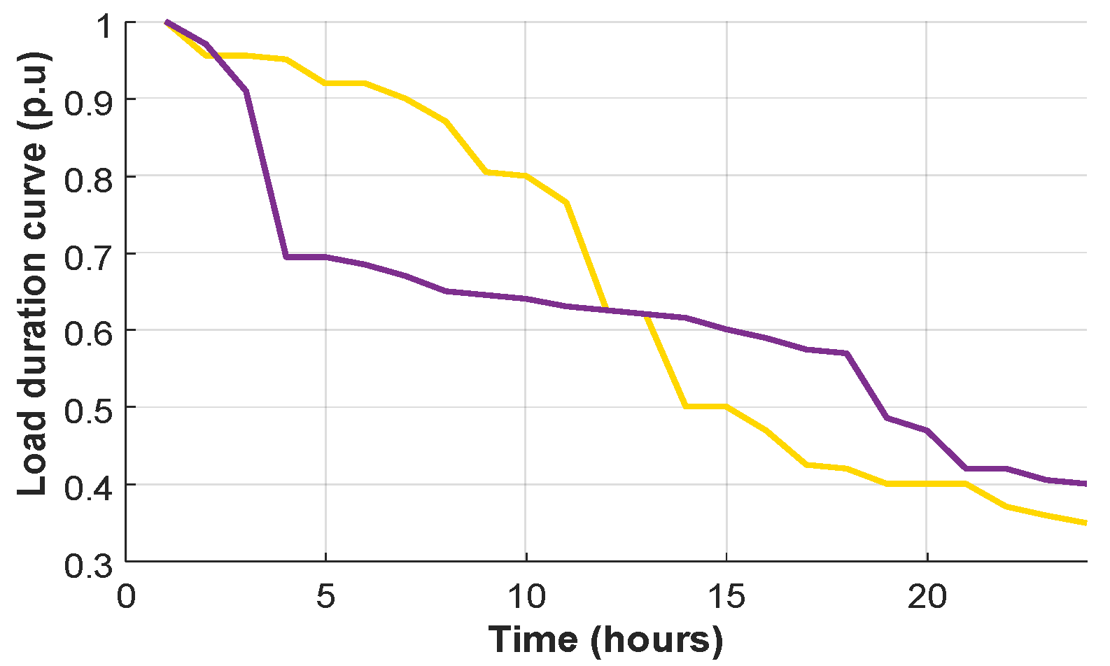
A different approach to represent the power consumption is to use the load duration curve (LDC), in which demand is organized and plotted in a descending order, starting from the highest power demand up to the lowest measured demand. Figure 2 shows the LDC pattern. This type of demand is frequently used to simulate the demand in tasks, such as the design and planning of distribution networks, as this would reduce the calculation time of the problem, which might be extremely longer in activities, such as long-term planning.
The scaling time used for the load duration curve (LDC) may be daily, weekly, monthly, or yearly, depending on the data availability and the objective of the study. Demand can be represented per unit or by using the value of the power demand.
2.2. Design and Planning of Power Distribution Networks and its Dependence on the Power Demand
Distribution networks are dynamic systems because of the continuous addition of customers to the network and their effect on the growth of power demand over time. Design and planning of the DN is focused on the expansion and the increase of the power capability because of the necessities of the network, which are necessary to meet the increased demand during its lifetime and to guarantee the supply of power required by the costumers.
The DN design criteria are strongly dependent on both the expected demand of the network and the capacity reserve, which is defined as an extra capacity that should be added over the required capacity of the feeders and assets to avoid power supply problems during the operation of the DN. This involves increasing the capacity of feeders by adding a percentage over the expected demand because the network should be able to deal with demands higher than the expected demands, which could produce differences with respect to the expected demand used in the planning aspect of the network.
These aspects, the peak demand and the reliability in the power supply, determine the maximum capacity of feeders and assets during the DN design. Therefore, the final capacity of feeders, protection, and assets will be higher than those required to meet the peak demand of the network.
2.3. Feeder Efficiency and its Dependence on the Demand Profile
This section of the article proposes a method to determine the efficiency of a DN by taking into account the effect of a daily load profile and the full capacity of the network. The method proposed uses two different indices to calculate both the single efficiency of every branch in the network and the overall exploitation capacity of the network.
The maximum capacity of feeders is calculated during the planning and the design process, and has to guarantee the network capacity required for managing the peak power demand during the operation of the DN while ensuring the reliability in the supply of power. Therefore, the network has to be able to use its maximum power capacity during 24 h of every day, the whole 365 days of the year, even if the power demand does not reach the available capacity.
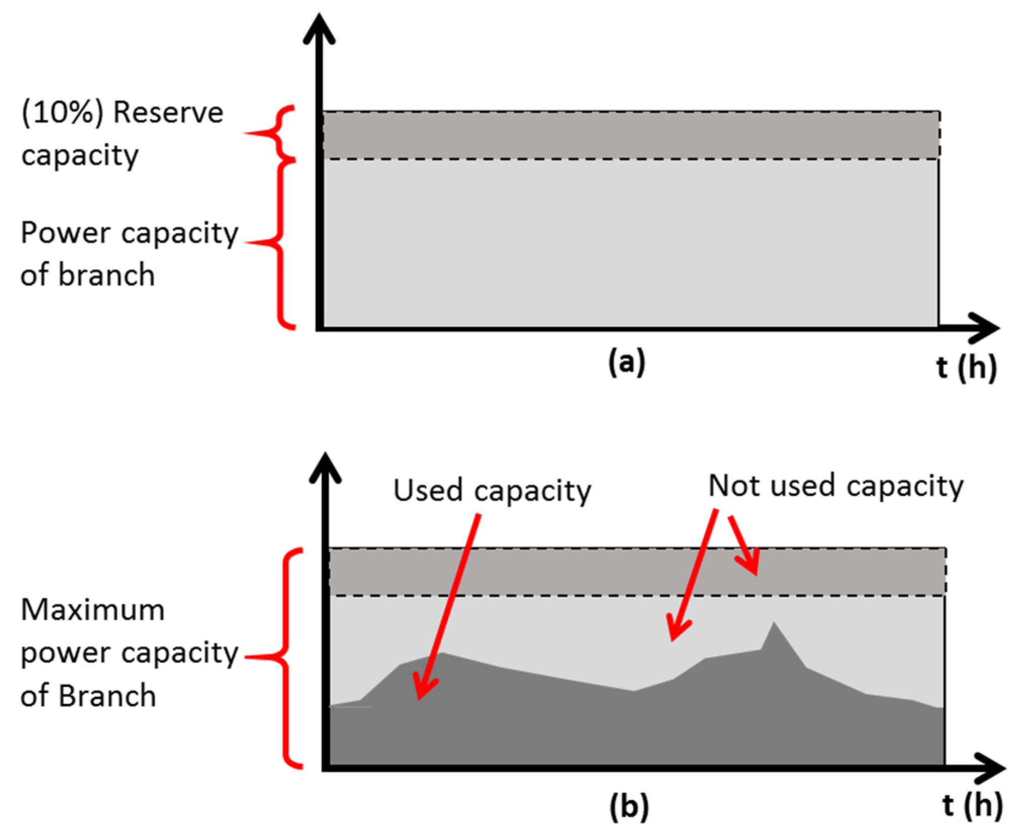
Figure 3 explains the meaning of the exploitation capacity concept, which refers to the proportion of the feeder’s capacity that is really used on an hourly basis within a representative day of the year, in relation of the full available capacity of the feeders. It is assumed that the used daily profile is a representative pattern of the demand consumption in the network. The exploited capacity is calculated as a percentage of the capacity of assets and the capacity of feeders that are effectively used during the operation in relation to the full capacity of assets and the full capacity of feeders.
The efficiency of every branch is calculated as the relation between the full available capacities of the respective elements in relation to its total capacity for each hour in a day.
Although the maximum power capacity of the feeder is always available, a typical DN operates at around 50% or 60% of its full capacity most of the time. Therefore, DN has a low exploitation level in relation to its full capacity, because there is a high portion of the capacity of the feeder not used along the day even though the assets are able to supply their maximum capacity. The exploitation capacity involves low efficiency when using assets and feeders during the daily operation of the DN. Despite this, it is almost impossible to improve the efficiency up to the highest possible levels because of the uncontrollable behavior of the demand. The continuous variation of the power demand throughout the day results in important changes in the operational conditions, which might cause negative effects on the operation of the network, in addition to the high requirements of capital investment for the expansion and repowering of DN.
Having considered these problems, a good option to improve the performance of DN and to reduce the total capital and operational costs is to control the demand during peak hours. To this end, it is necessary to calculate the efficiency of every feeder and asset of the network and then to identify the most relevant elements in its operation. Once the effect is identified, it is possible to calculate and analyze the best options to improve the operational conditions of the network.
Figure 3 shows how the full capacity of a feeder is defined based on the peak capacity required to meet the demand as well as the reserve capacity (extra capacity) required to ensure the reliability of the supply.
2.4. Exploitation Capacity of the Network
Valuation and analysis of the exploitation of resources in production systems are common practices in industrial companies. This practice aims to evaluate and improve the production-process efficiency when using the available resources as a way to improve the production capacity and to reduce the necessity of investment [33]. This common practice avoids the use of capital as a unique way to increase the production capacity as well as the profits of an industrial company. Some aspects that can be controlled and improved after the valuation of the efficiency are the production capacity of the process and the production capacity of the machinery. This valuation aims to determine the available capacity in every production process at any time and the marginal cost of production. Despite the differences between this kind of company and electric networks, there are some common aspects to be analyzed, such as the capacity of assets and their capital, and operational costs.
Distribution networks are constrained systems in which the feeders must deliver the power from the power substations to the final customers. However, in this case, feeders are not used efficiently due to the consumption habits of customers and some specific characteristics of the network, such as its maximum capacity of power delivery, the length of the feeders, and the distance between the supplying centers and the final customers. Additionally, it is necessary to make sure that the operational conditions of the network are within the right operational limits.
3. Proposed Exploitation Capacity of the Network
After identifying the importance of determining and managing the efficiency of the network as a way to improve the network behavior and a way to reduce the investment and operational costs, a new index to calculate the efficiency and the exploitation capacity of the network is proposed below.
3.1. Efficiency in the Use of the Feeder
The efficiency determines how the feeder capacity is used in a specific time. It is calculated as the relation between the power flow through the i,j feeder at a time in relation to the maximum capacity that the respective feeder has in the same year y. The equation is as follows:
The efficiency
varies in each of the three load blocks, but in this case, the demand consumption is represented by a three-level LDC.
3.2. Exploitation Capacity of the Feeders
The exploitation capacity of every feeder is calculated as the pondered sum of the feeder efficiency and represents the overall efficiency when using the feeder throughout the day in year y:
If there is a specific time “h” and each feeder delivers power that is exactly equal to its maximum power capacity, the exploitation capacity of the feeder will be equal to 1, so 100% is used efficiently every moment throughout the day. This is a hypothetical case that could be possible only if there is a unique load located in an extreme of the network and a source located in the opposite side of the network. Having explained that a distribution system is composed of several loads located in different load buses, all or most feeders will have an exploitation capacity lower than 1.
3.3. Exploitation Capacity of the Network
To calculate the total exploitation capacity of the DN, it is necessary to include the relevance of every feeder that composes the network into the index calculation. This involves the addition of a pondering factor for each feeder based on the relevance of the feeder during the operation of the network. Equations (3)–(5) describe the mathematical formulation of this index:
The pondering factor is calculated based on the power delivered through the feeder when the maximum peak of the demand occurs, so it is calculated as the rate between the power flowing through the feeder and the total power, which is supplied to the power transformer at the same time. To normalize the index significance, this value is divided into the sum of the power flows delivered by all the feeders at the same time.
As a result of including these parts of the index, the total exploitation capacity of the network is obtained as shown in Equation (3):
Equation (6) represents the total exploitation capacity of the network taking into account not only the efficiency in the use of the feeders but also the relevance of every feeder during the operation of the power distribution network.
3.4. Validation and Implementation of the Exploitation Capacity Index
To validate the proposed indices and their advantages to determine if the DN is used efficiently, a validation process is implemented based on the IEEE 13 bus distributions test system [34]. The validation process is developed by simulating three different cases in which the efficiency, the pondering factor, the exploitation capacity of feeders, and the exploitation capacity of the DN are calculated.
The first case uses a constant load that does not change during the 24 h of the day, connected only to a load bus, while the other buses do not have any load connected. The second case uses a unique load connected to the network, but in this case, the demand is simulated by a three-level load duration curve (LDC). The third case uses three-level LDCs to represent a power demand in each bus of the network.
Figure 4 shows the distribution test system used to validate the indices.
Case 1: This case includes a 5000 MVA load connected to bus 4 and a power source (transformer) connected to bus 1; they are the only two elements connected to the network. The load is simulated as a constant demand that does not change during the 24 h of the day.
In this case, there are three different branches (1-2, 2-3, and 3-4) delivering the power from the power source to the load bus, so each of the branches delivers almost the same power and has the same pondering factor. The sum of these pondering factors is equal to one, which proves that the factors were well assigned and added to reach the 100%.
The exploitation capacity of every feeder is calculated taking into account the maximum capacity that the feeder can supply during the 24 h of the day in relation to the total power that this branch delivers at the same time. This index is calculated using Equation (2).
Table 1 shows the pondering factor, the efficiency of the feeders, and the exploitation capacity of the branches in the first validation case.
The results correspond to the expected behavior of the system taking into account the characteristics of the DN and the type of the test, which model a unique load and a single source. This involves having a single path composed of three branches delivering the same power from the source to the load.
This proves that the pondering factor is well defined because the sum of the factors of the branches is equal to one. In the case of the efficiency and exploitation capacity, the index values are equal in the three branches because these branches deliver almost the same amount of power and have the same thermal capacity. Therefore, branches have the same relevance or importance in the supply of power from the main source to the load.
In this case, the exploitation capacity of the network is equal to the exploitation capacity of the branches. These results coincide with the expected values, based on the working regime of a network that operates with a single load and a single power source.
The exploitation capacity of the network is 0.736 and is close to the efficiency and the exploitation capacity of the branches. By analyzing the results, it is possible to conclude that the indices are well designed and reflect the operational condition of the network under the test conditions used in this case.
Case 2: This case simulates the same load location and the same source as in the previous case, but now the load is simulated as a three-level LDC (Load Duration Curve) as described in Table 2.
The results for case 2 are pondered as in case 1 because the feeder’s capacity and the load flowing through the feeders are equal for each time level (load block). The relevance of the feeder to the operation of the DN is then similar to the previous case.
On the other hand, the efficiency and exploitation capacity of the branches change compared with the values obtained in case 1. The efficiency changes because there are three different load levels while the branch capacity remains constant all the time. The usable capacity of branches is exploited in a less efficient way during the lowest demand levels (levels two and three in Table 3) than during level one because the supply of power use the lower feeder’s capacity during these levels compared to the capacity used during level one. The exploitation capacity of the branches decreases compared with the previous case due to the same reason. As a consequence of these changes, the exploitation capacity of the network also decreases.
The analysis of the indices for case 2 shows that the results are as expected again, because the efficiency of the branches decreases when the power flow decreases. This produces a reduction in the exploitation capacity of the network, which is a consequence of the low efficient use of the capacity of the branches throughout the whole day.
Case 3: This case simulates three-level LDCs for each of the 13 buses of the network. The time and per unit demand characteristics of LDC maintain the same values shown in Table 2 for all loads. Table 4 shows the peak power demanded in the buses.
The results for case 3 make it possible to demonstrate the pondering factor by using a fully loaded distribution network, as described in Equation (5). In this case, there are 12 branches in the distribution network delivering different power flows at the same time, which is a load condition different from the one tested in cases 1 and 2.
In this case, the pondering factors assign higher values for the branches that deliver more power during the peak hours as in branches 1-2 and 2-3, and assign low pondering values for the branches that deliver low power in relation to the total peak power demanded at that time. In this case, the pondering index assigns more relevance to the most congested branches because they are highly critical during the supply of power and more expensive than other branches that are not highly loaded. This kind of branch is usually found close to the main power source but could also be found in any other part of the DN if distributed generations were included.
The efficiency and the exploitation capacity of the branches are calculated and interpreted as in case 2. The obtained results and the validation results again demonstrate the validity of these indices to measure the whole working conditions of the branches and the distribution network (Table 5).
4. Mathematical Formulation of the Planning Problem
The problem simulated in this article is a 7-year planning problem in which the demand rises 3% per year in all buses.
The planning results indicate the potential upgrades in substations, feeders, and reactive compensators, including the year in which the upgrades should be installed, the optimal sizing, and the allocation of capacitor banks. The operational constraints limit the maximum power flows through branches and feeders, as well as the maximum and minimum voltages on the buses. The problem is formulated as a mathematical optimization problem and solved through GAMS software.
4.1. Objective Function
The objective function is the minimization of the total energy loses during the planning time and is represented by Equation (7):
where K is a variable that penalizes the number of devices installed during the planning solution by including a factor that increases the objective function when there are too many devices installed during the planning period. This variable penalizes the total number of feeder upgrades, the number of reactive compensators, and the number of capacitors that have to be installed during the planning of the network.
This penalization factor is necessary to avoid an extremely high number of units to be installed during the planning of the network because the objective function minimizes the total losses but does not restrict, by itself, the total number of elements to be installed in the network.
4.2. Operational Constraints
The operational constraints of the optimization problem under investigation are the power balance equations described by Equations (9) and (10) and the nodal voltage limits given by Equation (11):
4.3. Reactive Compensation Constraints
The size of the reactive compensators is obtained through Equation (12), where is the capacity of the units to be installed and is a variable that determines the number of units to be installed on a bus, while determines the cumulated capacity upgrade installed on yearly basis during the planning of the network. The reactive power supplied by the compensators is described by Equation (13). Another constraint is the maximum number of units that might be installed during the whole planning process as presented in Equation (14):
4.4. Constraints for Power Substation Upgrades
In the case of the substation, the upgrades are calculated by using binary variables that choose the capacities to be installed based on previously defined capacities: 100, 200, 500, 1000, and 1500 kVA. Equation (15) shows how the substation capacity required in year y is calculated based on the capacity in year y – 1 and the capacity to add, which is determined by choosing one or more of the five available possible size capacities by using a binary variable . The total capacity to add-in is the sum of the selected elements:
The active and reactive power supplied for the power substation (SS) are described by Equation (16) and Equation (17), respectively:
4.5. Constraints for Feeder Upgrades
Other elements to be upgraded during the planning of DN are the feeders, which should be upgraded if the power flowing through the branch is higher than its maximum power capacity (thermal capacity). In this case, the capacity of branches can be increased by steps of using an integer variable that determines the number of steps required to upgrade the branches as described by Equation (18):
The maximum active power and reactive power allowed on the feeder are described by Equation (19) and Equation (20), respectively:
In addition to the operational constraints of the planning problem, this problem includes the indices to calculate the efficiency and exploitation capacity of the DN and used these to correlate the peak demand variations to the branches’ efficiency and to the total cost of the network’s planning.
5. Case of Study and Test Results
This section shows and analyzes the results obtained for the planning problem in the four scenarios proposed by simulating the planning of a power distribution system through the use of the IEEE 33-bus distribution test system [35,36]. As indicated previously, the problem simulates four different cases of power demand, each for a different scenario and at a different peak demand.
5.1. Load Modeling for the Planning
5.1.1. Initial Conditions of the Distribution Network in Year-0
Table 6 shows the peak demand on the DN for the case PD100, which is used to calculate the starting conditions of the network in year-0.
Table 7 shows the power flow and the maximum power capacity of the branches when the demand is PD100. The branch capacities are calculated by taking into account the power flows through the feeders but including an additional 10% power over the required capacity. This is necessary to make sure that the branches are able to support the unexpected overloads.
5.1.2. Load Representation for the Planning Scenarios
The four LDCs represent different load conditions that could be created by managing the demand. It is assumed that it is possible to manage the demand and to modify the LDC PD100 to obtain different loads, such as the PD90, PD80, and PD70. This condition is necessary to compare and to evaluate the planning results; any other condition would not make it possible to compare the results. Table 8 shows the per-unit loads and times used to represent the LDCs.
Table 8 shows that the load demand is different in each of the blocks for the three LDCs. Level 1 represents the maximum demand in each case (90%, 80%, and 70% in relation to the load PD100), while levels 2 and 3 represent the demand in different load conditions and with different durations by block. The per-unit energy supplied is around 14.5 p.u., but this is only a reference value to ensure the LDCs are equivalent.
5.2. Planning Solution
The planning solution returns the necessary upgrade requirements that safeguard the operational conditions of the network during the 7-year planning period. Once the upgrade requirements and the total cost of the planning are obtained, the efficiency and the exploitation capacity of the network are calculated and compared.
The next part of the article presents and compares the results of the four scenarios proposed. By comparing these scenarios, it is possible to analyze the effect of the exploitation capacity of the network in terms of the planning cost as well as the effect of assets installed before the starting time of the planning period (Figure 5).
The proposed problem is an MINLP problem solved by using DICOP, CPLEX, and solvers, and it was run in GAMS software by minimizing the total energy losses for each of the four cases. The starting conditions of the network in year-0 are equal in the four cases, including the assets’ locations, assets’ capacities, and the network’s configuration. These aspects are obtained from year-0 in the reference case of the planning problem, which is the PD100 scenario. Having established this condition as the starting point of the planning, it is clear that the other cases (PD70, PD80, and PD90) do not use the full capacity of the network in year-0, and then the planning results are different even though the daily energy demand represented by the load duration curves is equal for the four scenarios.
5.2.1. Upgrade Solutions Obtained for the Four Scenarios
The results presented in Table 9, Table 10, and Table 11 show the different upgrade requirements for each scenario. The main scenario (PD100) demands a number of assets greater than the other cases. This scenario has to increase the supply capacity of the substation by installing 15 additional units of 100 MVA each, increasing the substation capacity to 1500 MVA respect to the capacity in year-0. On the other hand, scenario two needs eight units, while scenarios three and four need one unit each installed in year 7, as shown in Table 9.
As for the feeders, it is not necessary to increase their delivery capacity in scenarios PD70, PD80, and PD90, but it is essential to make three branch upgrades in scenario PD100 because of its higher peak demand compared with the other cases. In the scenario PD100, it is necessary to make a 200 MVA upgrade in branch 5-6 in year 2, the second upgrade of 400 MVA in branch 1-2 in year 3, and a 200 MVA final upgrade in branch 1-2 in year 4.
The last type of device that should be included in the planning is the reactive compensators, which allow the voltages to be within the right operational limits.
5.2.2. Effect of Losses in the Planning
According to Table 9, Table 10, and Table 11, a peak reduction in demand promotes better use of the network by increasing the efficiency in the use of the capacity of the feeder. Consequently, its useful lifetime rises.
This occurs because the mean available capacity of the branches increases due to the peak demand reduction and could lead to a more efficient use and a better exploitation capacity of the branches. Under this condition, the feeders can be used for a longer time, supporting the growing demand for more years than in other scenarios without increasing their maximum thermal capacities. This comprises additional advantages, such as the reduction in the capital investments necessary to ensure the power supply during the planning period.
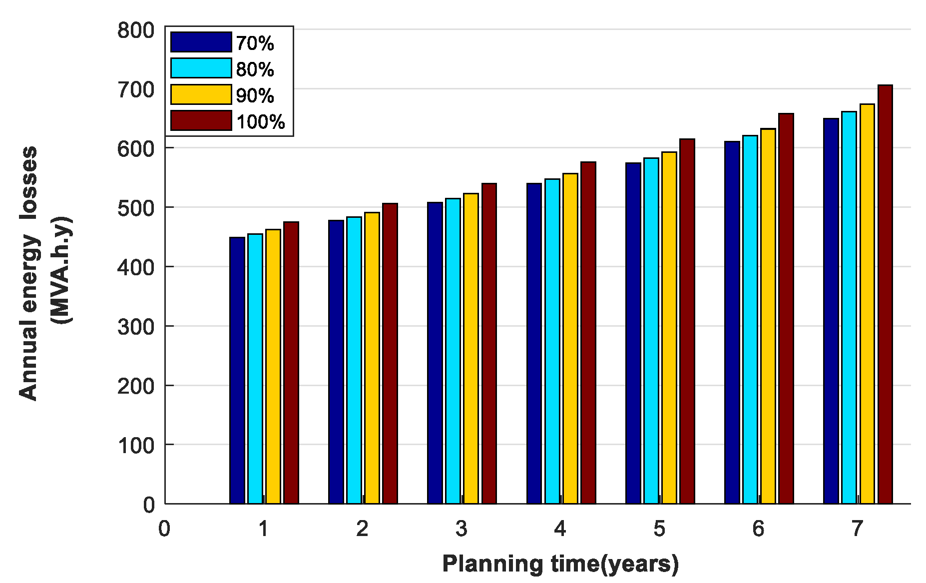
Figure 6 shows the differences between the total energy losses in the four scenarios. Losses increase yearly because of the rising peak demand. Figure 6 also shows the differences between the annual losses increases, which can be explained due to the differences in demand and the benefits obtained due to the upgrade of assets and the integration of new elements, such as reactive compensators. The behavior of losses coincides with the behavior expected because the largest losses appear when there are higher demands, whereas the lowest losses appear when there are lower demands. However, losses increase in scenarios PD70, PD80, and PD90 more slowly than in scenario PD100 because the investment in upgrades for these scenarios is more effective in reaching a reduction in energy losses.
Figure 7 shows the total energy losses during the whole planning period in the four scenarios. The total losses for scenario PD100 are 3.49% higher than scenario PD90, 5.15% higher than scenario PD80, and 6.48% higher than scenario PD70. In analyzing the results, it is clear that the first 10% reduction in the peak demand reduces losses by around 3.49%, the second 10% reduction (scenario PD80) decreases the losses an additional 1.72% with respect to the first case, and the third 10% reduction (scenario PD70) produces additional 1.4% losses reductions with respect to the second case.
6. Discussion: Efficiency of Feeders and Exploitation Capacity of the Network
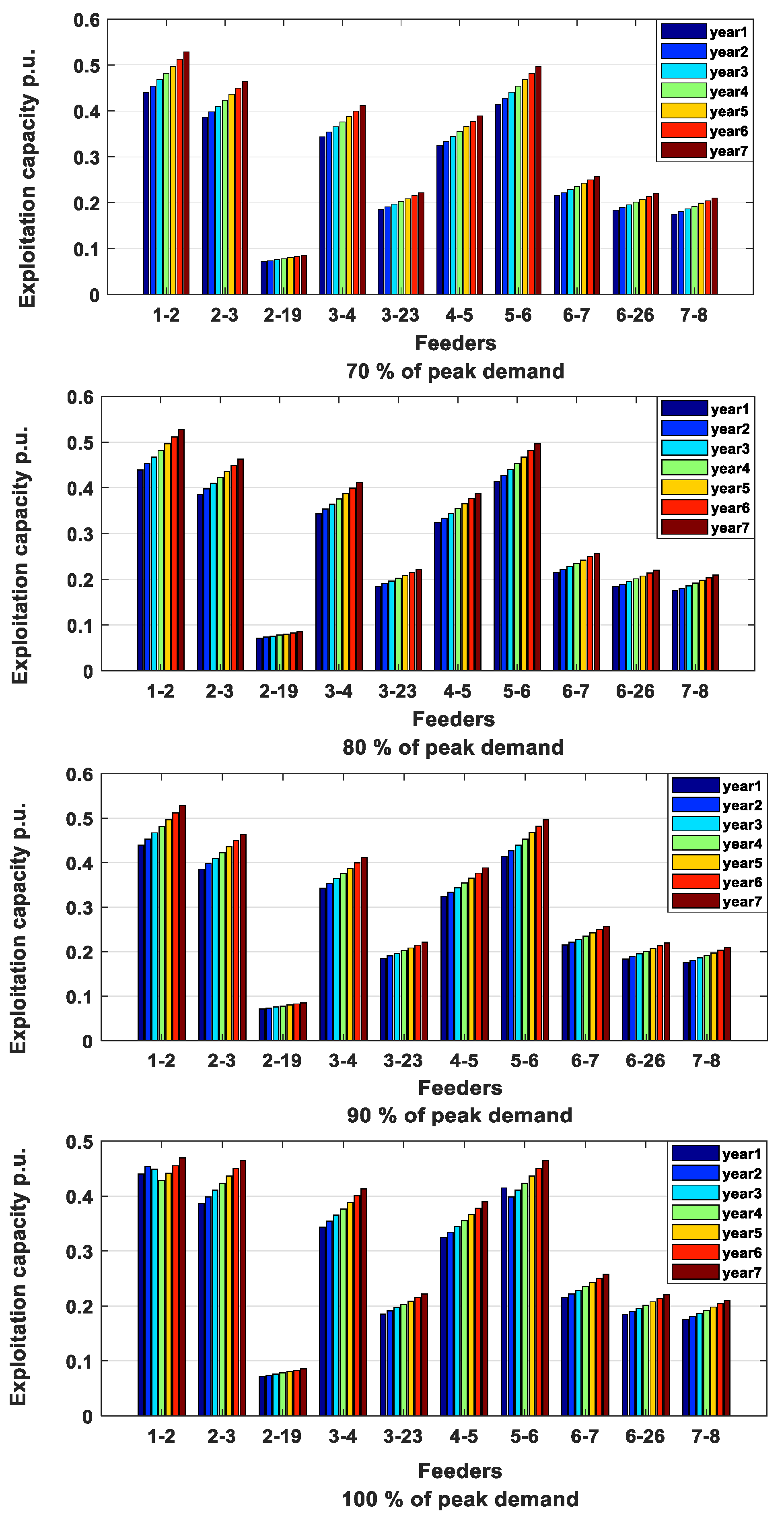
The efficiency of feeders is an important aspect that measures how the capacity of the branches is used for delivering power. As shown in Figure 8, most branches operate around or under 50% of their delivery capacity. The main reasons behind that are the difficulty of managing the demand and the remote location of some branches from the power substation, so these branches deliver very low power flows in their first operational years and consequently have low efficiency and low exploitation capacities.
This is a common case in distribution networks designed based on a classical concept of a centralized power substation and a radial distribution network that delivers power from the source to the customers.
Figure 8 shows 10 of the 32 feeders that compose the DN. According to this figure, some branches deliver low power, such as branch 2-19, but others deliver high power, such as branches 1-2 and 2-3. In this case, the highly loaded branches are the most important and expensive elements in the distribution network, in addition to the power source.
Figure 8 also shows how the efficiency in the use of branches increases along the planning horizon, with few differences in the four scenarios. This can be explained due to the growing demand, which is equal for every one of the buses, and therefore, there are no major differences when comparing the efficiency of the same bus in different years of the planning period.
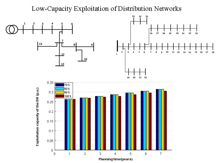
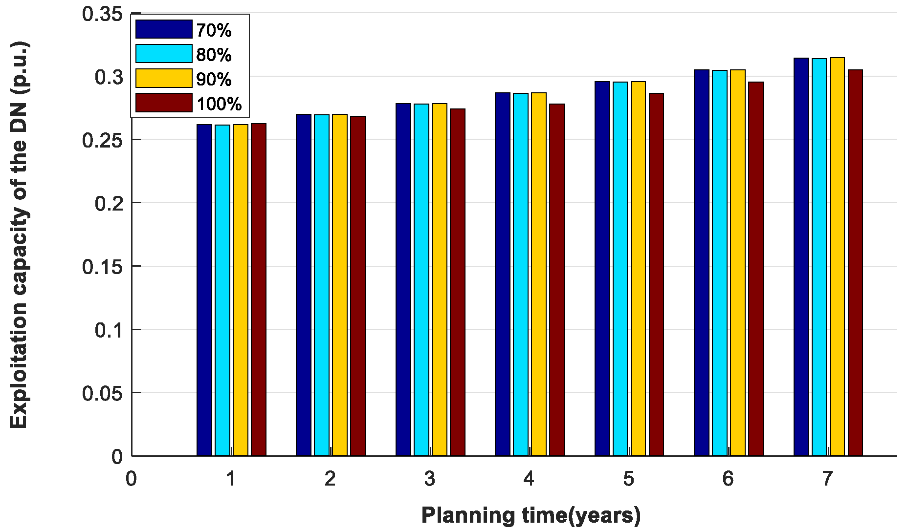
The analysis of the exploitation capacity of the network shows that all scenarios obtain similar values in year 1, but the exploitation capacity changes when years run one by one up until reaching year 7. Cases PD70, PD80, and PD90 show a similar exploitation capacity growing in the seven years of the planning period, but in case PD100, the exploitation capacity increases more slowly than in the other cases and become the lowest one in year 7.
This is resonated in scenario PD100, where the power flows rise faster than in the other scenarios and reach the maximum capacity of the branches in less time. Having met this condition, the branches must be upgraded, as shown in Table 10. In this specific case, the efficiency and the exploitation capacity of the branches improve before starting the upgrades, but after that, these indices decrease again because of the increase of the total available capacity of branches. Under this condition, the branches that are upgraded decrease their efficiency and this affects the exploitation capacity of the network.
In the other cases, there are no upgrades because the existing feeders have adequate available capacity, which can be exploited more efficiently compared with case PD100. In these scenarios, there are no extreme demand peaks as in scenario PD100, so the power demand is distributed more uniformly and efficiently over the 24 h of the day. This means that the available capacity of the feeders can be better exploited by increasing the use of the existing assets for a longer time while reducing the need for additional upgrades.
If the existing feeders are used more efficiently, major branch upgrades in the early years of the planning will not be necessary. As a consequence, the exploitation capacity of the DN of cases PD70, PD80, and PD90 increase in relation to the first years of the planning period but becomes higher than the exploitation capacity of DN in case PD100.
Additionally, the financial effects of the low efficiency in the use of the network can be explored. Once the scenarios about the efficiency and the exploitation capacity are analyzed, it is possible to correlate the requirement of capital investments, the efficiency of branches, and the exploitation capacity of the DN by analyzing the total cost of the solution for each scenario.
Table 12, Table 13, Table 14 and Table 15 summarize the planning cost for the scenarios proposed and include the fixed cost, the variable costs, and the cost of energy losses. Table 15 shows the total cost of the planning problem for the scenarios. According to the conducted comparison among various scenarios, scenario PD100 has higher energy losses and the most expensive solution. In addition, scenarios PD90, PD80, and PD70 produce savings of 35.86 million, 81.07 million, and 21.07 million dollars when compared to the planning cots for scenario PD100, respectively.
These results indicate that it is possible to improve the exploitation capacity of the network by using the branches more efficiently, in addition to reducing the requirements of the capital investments as well as the cost of energy losses.
Finally, it is possible to correlate a higher exploitation capacity index with a cheaper planning solution, because reducing the need for upgrades and the integration of new assets can be achieved by using the network more efficiently (Figure 9).
7. Conclusions: Effects of Low Exploitation Capacity during the Planning of Power Distribution Networks
Once the indices are validated, it is important to analyze the exploitation capacity of the DN and its relation to the planning of the DN. Then, it is necessary to find the relation between the planning solutions, the total cost of the planning, and the exploitation capacity of DN.
This evaluation is performed by running the planning on the IEEE 33-bus distribution network (see Figure 5 in Section 5), in which the assets composing the network in year 0 ensure their operational conditions when using a base-load demand named PD100. The maximum capacities of branches were previously defined based on the PD100 demand, represented by an LDC.
The valuation process runs and evaluates four different planning cases, each with different load demands. The load demands are represented by using different LDCs identified as PD100, PD90, PD80, and PD70 in which the peak demands are 100%, 90%, 80%, and 70%, respectively, of the base load. However, these LDCs supply the same amount of daily energy.
The LDCs named PD90, PD80, and PD70 reduce the peak demand to 90%, 80%, and 70%, respectively, in relation to the peak power demanded in the PD100 LDC. Despite the peak differences, the daily energy demanded by the LDCs is equal in the four cases and it is possible to compare the upgrade requirements for the different scenarios as well as the effects on the capital and the operational planning costs.
The exploitation capacity index proved to be a good tool to determine how efficiently the network is used in a whole typical day, based on the real used capacity and the maximum available capacity of the branches.
The mathematical formulation and the indices’ validation prove that the indices correctly interpret the different possible working states of the network, for example, the working condition based on a single load and a unique source.
The proposed pondering factor proves to be a well-defined tool to determine the importance of every branch in the operational condition of the network as well as in the overall valuation of the network efficiency.
It was demonstrated that the low exploitation capacity of the network is strongly related to a more expensive planning solution when planning starts working with a pre-existing distribution network with feeders and branches previously designed and specified for a high peak demand PD100.
Author Contributions
Conceptualization, J.A.A., S.R., F.S. and A.S.A.-S.; methodology, J.A.A., S.R. and F.S.; validation, J.A.A.; formal analysis, J.A.A., S.R., F.S. and A.S.A.-S.; investigation, J.A.A., S.R. and A.S.A.-S.; resources, J.A.A. and F.S.; data curation, F.S.; writing—original draft preparation, J.A.A., S.R. and F.S.; writing—review and editing, J.A.A., S.R. and A.S.A.-S.; visualization, F.S., J.A.A. and A.S.A.-S.; funding acquisition and supervision, F.S., S.R. and A.S.A.-S. All authors have read and agreed to the published version of the manuscript.
Funding
This research received no external funding.
Acknowledgments
The authors acknowledge to the Universidad Distrital Francisco Jose de Caldas, Colombia, for supporting this research through its PhD educational financial help and the Universidad Nacional de Colombia for its research support thought the advisor and help of the EMC-UN research group. Also, this research is supported by Khalifa University under Award FSU-2018-25.
Conflicts of Interest
The authors declare no conflict of interest.
Nomenclature
| i,j | Sets to identify the buses |
| b | Set for the number of blocks of the Load Duration Curve (LDC) |
| h | Set to identify the block of time in the LDC |
| y | Set for the year of the planning |
| Ssz | Set to identify the possible sizes of substation |
Variables
| Binary variable for choosing power substation (SS) upgrade | |
| Exploitation capacity of the network | |
| Exploitation capacity of feeders | |
| Maximum capacity of the feeder i,j | |
| Integer variable for choosing the reactive compensator (SC) to install in the bus i | |
| Integer variable for choosing the Fdr Upgrades | |
| Active power supplied by SS | |
| Peak power supplied by SS | |
| Active power demanded at bus i | |
| Reactive power supplied by SS | |
| Reactive power supplied by SCs | |
| Reactive power demanded at bus i | |
| Number of SS units to install in year y | |
| Power flow on feeder i,j in year y, and time h | |
| Peak power flow on feeder i,j, in year y | |
| Initial power capacity on feeder i,j | |
| Total feeder capacity on feeder i,j | |
| Total reactive power supplied for SC units | |
| Feeder upgrade capacity to install in year y | |
| Substation capacity upgrade to install in year y | |
| , | Voltage magnitude in buses i and j |
| Pondering factor of feeders | |
| Impedance angles for the i,j feeder | |
| Voltage angles on buses | |
| Feeders Efficiency |
Parameters
| Capacity of SS in the starting year | |
| Maximum number of SC units that can be installed during the planning. | |
| Power factor constraint for SS | |
| Power Factor constraint for feeders | |
| Reactive compensators installed before starting the planning | |
| Reserve capacity | |
| Predefined size for feeder upgrades KVA | |
| Predefined size for reactive compensators kVAR | |
| Admittance matrix | |
| Angle to restrict the power factor on the feeders | |
| Angle to define de power factor on the substation | |
| Time duration of LDC blocks |
References
- Wong, S.; Bhattacharya, K.; Fuller, J.D. Electric power distribution system design and planning in a deregulated environment. IET Gener. Transm. Distrib. 2009, 3, 1061–1078. [Google Scholar] [CrossRef]
- Al-Sumaiti, A.S.; Ahmed, M.H.; Salama, M. Residential load management under stochastic weather condition in developing countries. Electr. Power Compon. Syst. 2014, 42, 1452–1473. [Google Scholar] [CrossRef]
- El-Fouly, T.H.M.; Zeineldin, H.H.; El-Saadany, E.F.; Salama, M.M.A. A new optimization model for distribution substation siting, sizing, and timing. Int. J. Electr. Power Energy Syst. 2008, 30, 308–315. [Google Scholar] [CrossRef]
- Soroudi, A.; Ehsan, M. A distribution network expansion planning model considering distributed generation options and techo-economical issues. Energy 2010, 35, 3364–3374. [Google Scholar] [CrossRef] [Green Version]
- Riva Sanseverino, E.; Tran, Q.T.T.; Di Silvestre, M.L.; Doan, B.V.; Nguyen, N.Q. Voltage profile improvement for soc son’s low-voltage grid with high penetration of PV systems by optimizing the location of SVC devices. In Proceedings of the 2018 IEEE International Conference on Environment and Electrical Engineering and 2018 IEEE Industrial and Commercial Power Systems Europe (EEEIC/I&CPS Europe), Palermo, Italy, 12–15 June 2018; pp. 1–5. [Google Scholar]
- Ziari, I.; Ledwich, G.; Member, S.; Ghosh, A.; Platt, G. Integrated distribution systems planning to improve reliability under load growth. IEEE Trans. Power Deliv. 2012, 27, 757–765. [Google Scholar] [CrossRef]
- Borges, C.L.T.; Falcão, D.M. Optimal distributed generation allocation for reliability, losses, and voltage improvement. Int. J. Electr. Power Energy Syst. 2006, 28, 413–420. [Google Scholar] [CrossRef]
- Bucolo, M.; Buscarino, A.; Famoso, C.; Fortuna, L.; Frasca, M. Control of imperfect dynamical systems. Nonlinear Dyn. 2019, 98, 2989–2999. [Google Scholar] [CrossRef]
- Anastasiadis, A.G.; Kondylis, G.P.; Polyzakis, A.; Vokas, G. Effects of increased electric vehicles into a distribution network. Energy Proced. 2019, 157, 586–593. [Google Scholar] [CrossRef]
- Al Kaabi, S.S.; Zeineldin, H.H.; Khadkikar, V. Planning active distribution networks considering multi-DG configurations. IEEE Trans. Power Syst. 2014, 29, 785–793. [Google Scholar] [CrossRef]
- Johnson, B.J.; Starke, M.R.; Dimitrovski, A.D.; Ridge, O.; Ridge, O. Examining the potential impact of plug-in electric vehicles on residential sector power demand. In Proceedings of the 2015 IEEE Power & Energy Society General Meeting, Denver, Colorado, 26–30 July 2015; pp. 1–5. [Google Scholar]
- Soares, B.N.; Da Rosa Abaide, A.; Bernardon, D. Methodology for prioritizing investments in distribution networks electricity focusing on operational efficiency and regulatory aspects. In Proceedings of the 2014 49th International Universities Power Engineering Conference (UPEC), Cluj-Napoca, Romania, 2–5 September 2014; pp. 1–6. [Google Scholar]
- Baricevic, T.; Skok, M.; Zutobradic, S.; Wagmann, L. Identifying energy efficiency improvements and savings potential in Croatian energy networks. CIRED Open Access Proc. J. 2017, 2017, 2329–2333. [Google Scholar] [CrossRef]
- Ibrahim, S.H.; Baharun, A.; Chai, C.J. Efficient planning of electrical distribution system for consumers in Sarawak, Malaysia. J. Teknol. 2015, 1, 103–109. [Google Scholar]
- Morillo, J.L.; Perez, J.F.; Quijano, N.; Cadena, A. Planning open and closed-loop feeders with efficiency analysis. In Proceedings of the 2015 IEEE Eindhoven PowerTech, Eindhoven, The Netherlands, 29 June–2 July 2015. [Google Scholar]
- Zare, M.; Azizipanah-Abarghooee, R.; Hooshmand, R.A.; Malekpour, M. Optimal reconfigurattion of distribution systems by considering switch and wind turbine placements to enhance reliability and efficiency. IET Gener. Transm. Distrib. 2018, 12, 1271–1284. [Google Scholar] [CrossRef]
- Vitorino, R.M.; Neves, L.P.; Jorge, H.M. Network reconfiguration to improve reliability and efficiency in distribution systems. In Proceedings of the 2009 IEEE Bucharest PowerTech, Bucharest, Romania, 28 June–2 July 2009; pp. 1–7. [Google Scholar]
- Padilha-Feltrin, A.; Quijano Rodezno, D.A.; Mantovani, J.R.S. Volt-VAR multiobjective optimization to peak-load relief and energy efficiency in distribution networks. IEEE Trans. Power Deliv. 2015, 30, 618–626. [Google Scholar] [CrossRef]
- Sanseverino, E.R.; Tran, Q.T.T.; Roose, L.R.; Sadoyama, S.T.; Tran, T.; Doan, B.V.; Nguyen, N.H. Optimal placements of SVC devices in low voltage grids with high penetration of PV systems. In Proceedings of the 2018 9th IEEE International Symposium on Power Electronics for Distributed Generation Systems (PEDG), Charlotte, NC, USA, 25–28 June 2018; pp. 1–6. [Google Scholar]
- Syahputra, R.; Robandi, I.; Ashari, M. Distribution network efficiency improvement based on fuzzy multi-objective method. IPTEK J. Proc. Ser. 2014, 1, 224–229. [Google Scholar] [CrossRef]
- Koutsoukis, N.C.; Siagkas, D.O.; Georgilakis, P.S.; Hatziargyriou, N.D. Online reconfiguration of active distribution networks for maximum integration of distributed generation. IEEE Trans. Autom. Sci. Eng. 2017, 14, 437–448. [Google Scholar] [CrossRef]
- Lakshmi, S.; Ganguly, S. Modelling and allocation of open-UPQC-integrated PV generation system to improve the energy efficiency and power quality of radial distribution networks. IET Renew. Power Gener. 2018, 12, 605–613. [Google Scholar] [CrossRef]
- Quijano, D.A.; Wang, J.; Sarker, M.R.; Padilha-Feltrin, A. Stochastic assessment of distributed generation hosting capacity and energy efficiency in active distribution networks. IET Gener. Transm. Distrib. 2017, 11, 4617–4625. [Google Scholar] [CrossRef] [Green Version]
- Zhao, J.; Wang, Y.; Song, G.; Li, P.; Wang, C.; Wu, J. Congestion management method of low-voltage active distribution networks based on distribution locational marginal price. IEEE Access 2019, 7, 32240–32255. [Google Scholar] [CrossRef]
- Bach Andersen, P.; Hu, J.; Heussen, K. Coordination strategies for distribution grid congestion management in a multi-actor, multi-objective setting. In Proceedings of the 2012 3rd IEEE PES Innovative Smart Grid Technologies Europe (ISGT Europe), Berlin, Germany, 14–17 October 2012; pp. 1–8. [Google Scholar]
- Yan, X.; Li, R. Flexible coordination optimization scheduling of active distribution network with smart load. IEEE Access 2020, 8, 59145–59157. [Google Scholar] [CrossRef]
- Quadri, I.A.; Bhowmick, S.; Joshi, D. Multi-objective approach to maximise loadability of distribution networks by simultaneous reconfiguration and allocation of distributed energy resources. IET Gener. Transm. Distrib. 2018, 12, 5700–5712. [Google Scholar] [CrossRef]
- Kroposki, B.; Sen, P.K.; Malmedal, K. Selection of distribution feeders for implementing distributed generation and renewable energy applications. IEEE Trans. Ind. Appl. 2013, 49, 2825–2834. [Google Scholar] [CrossRef]
- Dashti, R.; Afsharnia, S. Demand response regulation modeling based on distribution system asset efficiency. Electr. Power Syst. Res. 2011, 81, 667–676. [Google Scholar] [CrossRef]
- Ye, L.; Hu, Z.; Li, C.; Zhang, Y.-J.; Zhang, S.; Yang, Z.; Zhang, D. The reasonable range of life cycle utilization rate of distribution network equipment. IEEE Access 2018, 6, 23948–23959. [Google Scholar] [CrossRef]
- Ma, L.; Liu, W.; Chen, H.; Cui, Y.; Wang, Y.; Yuan, S. Operation efficiency evaluation frame and its criteria for distribution network based on annual load duration curve. In Proceedings of the International Conference on Innovative Smart Grid Technologies (ISGT Asia 2018), Singapore, 22–25 May 2018; pp. 373–378. [Google Scholar]
- Zhang, W. Indices system and improvement measures of distribution network equipment utilization rate considering PV connection. In IOP Conference Series: Materials Science and Engineering; IOP Publishing: Bristol, UK, 2018; Volume 452. [Google Scholar]
- Luftig, J.T. Total Asset Utilization (TAU): An overview of a productivity metric for profitability enhancement and focused cost reduction. Meas. Bus. Excell 1997, 3, 20–25. [Google Scholar] [CrossRef]
- Aref, A.; Davoudi, M.; Razavi, F.; Davoodi, M. Optimal DG placement in distribution networks using intelligent systems. 2012, 2012, 92–98. Energy Power Eng. 2012, 2012, 92–98. [Google Scholar] [CrossRef] [Green Version]
- Wang, H.; Yan, Z.; Xu, X.; He, K. Evaluating influence of variable renewable energy generation on islanded microgrid power flow. IEEE Access 2018, 6, 71339–71349. [Google Scholar] [CrossRef]
- Alvarez, D.L.; Al-Sumaiti, A.S.; Rivera, S.R. Estimation of an optimal PV panel cleaning strategy based on both annual radiation profile and module degradation. IEEE Access 2020, 4, 1–8. [Google Scholar] [CrossRef]
Figure 1.
Residential (purple) and industrial (yellow) typical daily load profiles.

Figure 2.
Load duration curves for residential (purple) and industrial (yellow) sectors.

Figure 3.
(a) Graphical representation of the maximum power capacity of branches showing the power capacity in axis y and the hourly time in axis x. (b) Explanation of the daily exploitation capacity of DN (Distribution Network), based on the maximum power capacity of branches, and the hourly used capacity.

Figure 4.
Modified IEEE 13-bus test distribution system used to validate the indices [34].
Figure 4.
Modified IEEE 13-bus test distribution system used to validate the indices [34].

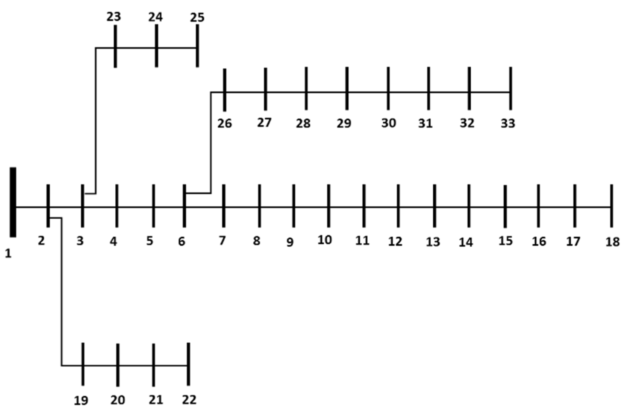
Figure 5.
IEEE 33 buses distribution test system, used to simulate and evaluate the effect of the feeder efficiency and the exploited capacity of the DN.
Figure 5.
IEEE 33 buses distribution test system, used to simulate and evaluate the effect of the feeder efficiency and the exploited capacity of the DN.

Figure 6.
Annual energy losses obtained in the four proposed scenarios.

Figure 7.
Total energy losses for the planning in each of the scenarios simulate.

Figure 8.
Annual variation of the exploitation capacity of the network in the four scenarios analyzed.
Figure 8.
Annual variation of the exploitation capacity of the network in the four scenarios analyzed.

Figure 9.
Annual variation of the exploitation capacity of the network in the four scenarios analyzed.
Figure 9.
Annual variation of the exploitation capacity of the network in the four scenarios analyzed.


Table 1.
Indices calculated for the validation test in the case 1.
| Feeder | Pondering Factor | Efficiency of Feeder | Exploitation Capacity of Feeder |
|---|---|---|---|
| “1-2” | 0.335 | 0.7414 | 0.7414 |
| “2-3” | 0.333 | 0.7359 | 0.7359 |
| “3-4” | 0.331 | 0.7304 | 0.7304 |
Table 2.
Load duration curve information used for the simulation.
| Levels | Demand (p.u.) | Demand (MVA) | Time (h) |
|---|---|---|---|
| Level 1 | 1.00 | 5000 | 2.5 |
| Level 2 | 0.62 | 3100 | 15.5 |
| Level 3 | 0.40 | 2000 | 6.0 |
Table 3.
Results of the validation process, case 2.
| Feeder | Load Level | Pondering Factor | Efficiency of Feeders | Exploitation Capacity of Feeders |
|---|---|---|---|---|
| “1-2” | Level 1 | 0.335 | 0.7414 | 0.4455 |
| Level 2 | 0.4567 | |||
| Level 3 | 0.2935 | |||
| “2-3” | Level 1 | 0.333 | 0.7359 | 0.4434 |
| Level 2 | 0.4546 | |||
| Level 3 | 0.2927 | |||
| “3-4” | Level 1 | 0.3308 | 0.7304 | 0.4413 |
| Level 2 | 0.4525 | |||
| Level 3 | 0.2918 |
Table 4.
Peak load demanded in the 13 buses of the DN.
| Bus Number | P (kVA) | Q (kVAR) | Bus Number | P (kVA) | Q (kVAR) |
|---|---|---|---|---|---|
| 1 | 0 | 0 | 8 | 460 | 145 |
| 2 | 445 | 234 | 9 | 383 | 249 |
| 3 | 314 | 235 | 10 | 331 | 240 |
| 4 | 556 | 382 | 11 | 345 | 93 |
| 5 | 318 | 189 | 12 | 646 | 277 |
| 6 | 237 | 172 | 13 | 562 | 240 |
| 7 | 671 | 539 |
Table 5.
Results of the validation process for case three.
| Feeder | Pondering Factor | Efficiency of Feeders | Exploitation Capacity of Feeders |
|---|---|---|---|
| “1-2” | 0.2035 | 0.7899 | 0.4728 |
| “2-3” | 0.1847 | 0.7167 | 0.4304 |
| “3-4” | 0.1711 | 0.6639 | 0.4000 |
| “4-5” | 0.1498 | 0.7611 | 0.4587 |
| “5-6” | 0.0089 | 0.0776 | 0.0469 |
| “5-7” | 0.1283 | 0.6521 | 0.3935 |
| “7-8” | 0.0442 | 0.3848 | 0.2325 |
| “7-11” | 0.0373 | 0.3247 | 0.1962 |
| “7-13” | 0.0211 | 0.1840 | 0.1112 |
| “8-9” | 0.0144 | 0.1254 | 0.0758 |
| “8-10” | 0.0124 | 0.1084 | 0.0655 |
| “11-12” | 0.0243 | 0.2116 | 0.1279 |
Table 6.
Power demand in the buses of the network when the simulated demand is PD100.
| Bus | P (kW) | Q (kVAR) | Bus | P (kW) | Q (kVAR) |
|---|---|---|---|---|---|
| 1 | 0 | 0 | 18 | 90 | 40 |
| 2 | 100 | 60 | 19 | 90 | 40 |
| 3 | 90 | 40 | 20 | 90 | 40 |
| 4 | 120 | 80 | 21 | 90 | 40 |
| 5 | 60 | 30 | 22 | 90 | 40 |
| 6 | 60 | 20 | 23 | 90 | 50 |
| 7 | 200 | 100 | 24 | 420 | 200 |
| 8 | 200 | 100 | 25 | 420 | 200 |
| 9 | 60 | 20 | 26 | 60 | 25 |
| 10 | 60 | 20 | 27 | 60 | 25 |
| 11 | 45 | 30 | 28 | 60 | 20 |
| 12 | 60 | 35 | 29 | 120 | 70 |
| 13 | 60 | 35 | 30 | 200 | 600 |
| 14 | 120 | 80 | 31 | 150 | 70 |
| 15 | 60 | 10 | 32 | 210 | 100 |
| 16 | 60 | 20 | 33 | 60 | 40 |
| 17 | 60 | 20 |
Table 7.
Maximum capacity of the feeders calculated based on the PD100 demand.
| Branch | Power Flow for PD100 (kVA) | Max Capacity of Branch (kVA) | Branch | Power Flow for PD100 (kVA) | Max Capacity of Branch (kVA) |
|---|---|---|---|---|---|
| 1-2 | 4613.0 | 5238.0 | 17-18 | 98.5 | 3055.0 |
| 2-3 | 4091.0 | 5238.0 | 2-19 | 395.3 | 3055.0 |
| 3-4 | 2901.7 | 4037.0 | 19-20 | 296.8 | 3055.0 |
| 4-5 | 2735.4 | 4037.0 | 20-21 | 197.0 | 3055.0 |
| 5-6 | 2648.5 | 3055.0 | 21-22 | 98.5 | 3055.0 |
| 6-7 | 1215.7 | 3055.0 | 3-23 | 1045.2 | 3055.0 |
| 7-8 | 987.7 | 3055.0 | 23-24 | 937.9 | 3055.0 |
| 8-9 | 759.7 | 3055.0 | 24-25 | 466.5 | 3055.0 |
| 9-10 | 691.1 | 3055.0 | 6-26 | 1361.3 | 3055.0 |
| 10-11 | 624.3 | 3055.0 | 26-27 | 1298.2 | 3055.0 |
| 11-12 | 569.9 | 3055.0 | 27-28 | 1236.5 | 3055.0 |
| 12-13 | 499.8 | 3055.0 | 28-29 | 1167.2 | 3055.0 |
| 13-14 | 428.1 | 3055.0 | 29-30 | 1026.9 | 3055.0 |
| 14-15 | 285.9 | 3055.0 | 30-31 | 472.3 | 3055.0 |
| 15-16 | 226.0 | 3055.0 | 31-32 | 304.1 | 3055.0 |
| 16-17 | 161.6 | 3055.0 | 32-33 | 72.1 | 3055.0 |
Table 8.
Information on load duration curves used for the load representation of demand in the different scenarios.
Table 8.
Information on load duration curves used for the load representation of demand in the different scenarios.
| LDC | Block of Load | Demand (p.u.) | Time (h) |
|---|---|---|---|
| 90PD | Level 1 | 0.900 | 2.6 |
| Level 2 | 0.635 | 15.0 | |
| Level 3 | 0.410 | 6.4 | |
| 80PD | Level 1 | 0.800 | 3.2 |
| Level 2 | 0.645 | 14.2 | |
| Level 3 | 0.420 | 6.6 | |
| 70PD | Level 1 | 0.700 | 4.5 |
| Level 2 | 0.655 | 13.0 | |
| Level 3 | 0.440 | 6.5 |
Table 9.
Substation upgrades required for each studied scenario.
| Year | Peak Level | |||
|---|---|---|---|---|
| 100% | 90% | 80% | 70% | |
| Y1 | 5 | 0 | 0 | 0 |
| Y2 | 0 | 0 | 0 | 0 |
| Y3 | 2 | 1 | 0 | 0 |
| Y4 | 2 | 2 | 0 | 0 |
| Y5 | 2 | 1 | 0 | 0 |
| Y6 | 2 | 2 | 0 | 0 |
| Y7 | 2 | 2 | 1 | 1 |
Table 10.
Feeder upgrades required to ensure the power supply in each scenario (70%, 80%, 90%, and the main case 100%).
Table 10.
Feeder upgrades required to ensure the power supply in each scenario (70%, 80%, 90%, and the main case 100%).
| Peak Level | Year | Branch | Capacity (p.u.) | Capacity (MVA) |
|---|---|---|---|---|
| 70% | NA | 0 | 0 | 0 |
| 80% | NA | 0 | 0 | 0 |
| 90% | NA | 0 | 0 | 0 |
| 100% | Y2 | 5-6 | 1 | 200 |
| Y3 | 1-2 | 2 | 400 | |
| Y4 | 1-2 | 1 | 200 |
Table 11.
Reactive compensation upgrades installed in each bus and the year when assets should be installed.
Table 11.
Reactive compensation upgrades installed in each bus and the year when assets should be installed.
| Peak Level | Year | Bus Installed Capacity (p.u.) | Total | ||
|---|---|---|---|---|---|
| B6 | B17 | B18 | |||
| 70% | Y1 | 5 | 0 | 2 | 7 |
| Y2 | 5 | 0 | 0 | 0 | |
| 80% | NA | NA | 1 | NA | NA |
| 90% | Y2 | 0 | 2 | 0 | 2 |
| 100% | Y1 | 0 | 1 | 1 | 1 |
| Y2 | 0 | 2 | 0 | 1 | |
Table 12.
Fixed cost of the planning solutions for each scenario proposed.
| Type of Upgrade | Fix Cost (USD) | Required Units for the Upgrading | |||
|---|---|---|---|---|---|
| 100% | 90% | 80% | 70% | ||
| Substation upgrades (units) | 200,000 | 2 | 1 | - | - |
| Feeder Upgrades (km feeders) | 150,000 | 0.40 | - | - | - |
| Reactive compensator (units) | 2 | 2 | - | 12 | |
| TOTAL CAPITAL COST (millions USD) | 0.460 | 0.200 | - | - | |
Table 13.
Variable cost of the planning solutions for each scenario proposed.
| Type of Upgrade | Var. Cost (USD) | Installed Capacity of Upgrades | |||
|---|---|---|---|---|---|
| 100% | 90% | 80% | 70% | ||
| Substation upgrades (MVA) | 50,000 | 1500 | 800 | 100 | 100 |
| Feeder Upgrades (MVA) | 1000 | 600 | - | - | - |
| Compensation upgrades (MVAR) | 50,000 | 200 | 200 | - | 1200 |
| TOTAL VARIABLE COST (millions USD) | 85.60 | 50.00 | 5.00 | 65.00 | |
Table 14.
Cost of the energy losses throughout the whole period of planning for the four scenarios proposed.
Table 14.
Cost of the energy losses throughout the whole period of planning for the four scenarios proposed.
| Total Losses During Planning | Energy Loss | Total Energy Losses during Planning (MVA) | |||
|---|---|---|---|---|---|
| 100% | 90% | 80% | 70% | ||
| Total energy losses US/MVA | 30 | 4073.17 | 3931.10 | 3863.49 | 3809.22 |
| COST OF LOSSES (millions USD) | 0.1222 | 0.1179 | 0.1159 | 0.1143 | |
Table 15.
Total costs of the planning in the four scenarios proposed.
| Total Cost of Planning | Cap Cost (USD) | Total Energy Losses during Planning (MVA) | |||
|---|---|---|---|---|---|
| 100% | 90% | 80% | 70% | ||
| Total planning cost | 86.18 | 50.32 | 5.12 | 65.11 | |
| Savings | - | 35.86 | 81.07 | 21.07 | |
© 2020 by the authors. Licensee MDPI, Basel, Switzerland. This article is an open access article distributed under the terms and conditions of the Creative Commons Attribution (CC BY) license (http://creativecommons.org/licenses/by/4.0/).
Share and Cite
MDPI and ACS Style
Alarcon, J.A.; Santamaria, F.; Al-Sumaiti, A.S.; Rivera, S. Low-Capacity Exploitation of Distribution Networks and Its Effect on the Planning of Distribution Networks. Energies 2020, 13, 1920. https://doi.org/10.3390/en13081920
AMA Style
Alarcon JA, Santamaria F, Al-Sumaiti AS, Rivera S. Low-Capacity Exploitation of Distribution Networks and Its Effect on the Planning of Distribution Networks. Energies. 2020; 13(8):1920. https://doi.org/10.3390/en13081920
Chicago/Turabian StyleAlarcon, Jorge A., Francisco Santamaria, Ameena S. Al-Sumaiti, and Sergio Rivera. 2020. "Low-Capacity Exploitation of Distribution Networks and Its Effect on the Planning of Distribution Networks" Energies 13, no. 8: 1920. https://doi.org/10.3390/en13081920
Note that from the first issue of 2016, this journal uses article numbers instead of page numbers. See further details here.