Wind Resource Assessment for Alaska’s Offshore Regions: Validation of a 14-Year High-Resolution WRF Data Set
by
 , ,
, ,
Jared A. Lee
1,* ,
,
Paula Doubrawa
2 ,
,
Lulin Xue
1,*,
Andrew J. Newman
1,
Caroline Draxl
2 and
George Scott
2 1
Research Applications Laboratory, National Center for Atmospheric Research, Boulder, CO 80307, USA
2
National Renewable Energy Laboratory, Golden, CO 80401, USA
*
Authors to whom correspondence should be addressed.
Energies 2019, 12(14), 2780; https://doi.org/10.3390/en12142780
Submission received: 30 May 2019
/
Revised: 11 July 2019
/
Accepted: 17 July 2019
/
Published: 19 July 2019
(This article belongs to the Section A3: Wind, Wave and Tidal Energy)
Abstract
:Offshore wind resource assessments for the conterminous U.S. and Hawai’i have been developed before, but Alaska’s offshore wind resource has never been rigorously assessed. Alaska, with its vast coastline, presents ample potential territory in which to build offshore wind farms, but significant challenges have thus far limited Alaska’s deployment of utility-scale wind energy capacity to a modest 62 MW (or approximately 2.7% of the state’s electric generation) as of this writing, all in land-based wind farms. This study provides an assessment of Alaska’s offshore wind resource, the first such assessment for Alaska, using a 14-year, high-resolution simulation from a numerical weather prediction and regional climate model. This is the longest-known high-resolution model data set to be used in a wind resource assessment. Widespread areas with relatively shallow ocean depth and high long-term average 100-m wind speeds and estimated net capacity factors over 50% were found, including a small area near Alaska’s population centers and the largest transmission grid that, if even partially developed, could provide the bulk of the state’s energy needs. The regional climate simulations were validated against available radiosonde and surface wind observations to provide the confidence of the model-based assessment. The model-simulated wind speed was found to be skillful and with near-zero average bias (−0.4–0.2 m s−1) when averaged over the domain. Small sample sizes made regional validation noisy, however.
1. Introduction
Wind power is a steadily growing source of energy generation in the United States and around the world. In 2017, wind turbines provided 515 GW, or about 4%, of generating capacity globally, with 18 GW of that being offshore wind [1]. By the end of 2016, wind turbines provided 82.1 GW of generating capacity in the United States, or 8% of the nationwide total, surpassing the generating capacity of hydroelectric power for the first time ever [2,3]. All but 30 MW of that capacity is from onshore wind farms, as the first (and as of this writing, still the only) operational offshore wind farm in the U.S. began production in December 2016 off the coast of Rhode Island [4]. A recent report by the National Renewable Energy Laboratory (NREL) estimated the nationwide total technical offshore wind energy potential capacity to be 2057 GW [5], revealing the tremendous and essentially untapped potential for new development to continue increasing wind power capacity in the U.S. That study and total estimate did not include Alaska, however, for technical reasons.
Alaska, despite its enormous geographical area, only has a modest 62 MW of installed wind capacity, all of it land-based, accounting for 2.7% of Alaska’s energy generation in 2016 [2]. By contrast, 48.0% of Alaska’s utility-scale net electric generation in 2016 was by natural gas, 26.2% by hydroelectric, 13.1% from petroleum liquids, 9.4% from coal, and 0.7% from biomass [6]. While only 29.5% of Alaska’s utility-scale net electric generation was from renewable energy sources in 2016, the Alaska State Legislature in 2010 adopted an uncodified (non-binding) goal of 50% renewable energy generation by 2025 [7]. To meet that ambitious goal, rapidly expanding wind power penetration will potentially play a prominent role.
There are several physical challenges to the expansion of wind power in Alaska, however. These challenges include rugged topography, sparse population, a harsh winter climate (including turbine icing), and an economy that continues to be heavily dependent on oil production. Another challenge is the fragmented and underdeveloped nature of Alaska’s power grid. The Alaska Grid (also known as the Railbelt Grid) serves Alaska’s main population centers of Anchorage, Fairbanks, and the Kenai Peninsula, but the remaining 86% of the state’s land area is serviced by small, independent, and often isolated transmission networks [8]. The isolated nature of these rural transmission networks, which are often powered by diesel generators served by intermittent, weather-dependent deliveries of diesel by road, barge, or small plane, leads to high electricity costs that are four to five times as expensive as that available in urban areas from the Alaska Grid, which are more competitive with prices in the conterminous United States (CONUS) [9]. These high electricity prices provide potential openings for new wind power development in Alaska in the future, including from offshore farms. The first step in determining potential feasibility of new offshore wind farms is to perform and validate a wind resource assessment. As Musial et al. [5] assessed the wind resource for the entire U.S. except Alaska, there is a need for an offshore wind resource assessment and validation for Alaska.
A wind resource assessment is merely the first step in a chain of events that must happen before a site suitable for a wind farm could be identified and developed. After a regional, model-based wind resource assessment is conducted from the hub-height wind speed, then candidate sites with suitably high average hub-height wind speed can be identified. The minimum average wind speed that is potentially economically viable will vary with the class of wind turbine and the current/predicted cost of electricity in the region, but is generally at least 5 m s−1, and often higher. Knowledge of the long-term average wind speed, coupled with considerations of favorable topography (or, for offshore sites, bathymetry), along with proximity to existing transmission infrastructure, will be the most important factors in identifying candidate sites.
Once candidate sites for wind farms are chosen, detailed measurement campaigns of at least one year in duration must be undertaken, usually from a met mast or LIDAR. This step is challenging offshore. The goal of the measurement campaign at specific sites is to obtain (near-) hub-height and rotor-layer wind speed information over each season, so that annual energy production at that site can be assessed. Met masts or LIDARs can also provide useful information not only about hub-height wind speed, but also about the profile of wind speed with height at that location, along with information about the turbulence. Accounting for the microscale turbulence characteristics, as well as wakes from other turbines upstream, is an important step to improve the accuracy and fidelity of a site-specific wind resource assessment (e.g., [10,11,12]). Additionally, studies of the adequacy of existing or new transmission lines to bring energy from the proposed wind farm to the rest of the grid must be conducted. In many cases, environmental impact studies must also be performed. Banks often require much of this information before extending financing for a proposed wind project. This study focuses on a regional wind resource assessment for the Alaska region, namely of the hub height wind speed, validated against available observations. The other steps in the process to obtain a bankable wind resource assessment for a specific site are outside the scope of this study and not discussed further.
In order to perform a wind resource assessment for a region as large as Alaska’s offshore zone, the primary options are either to use an atmospheric reanalysis product or to run a numerical weather prediction (NWP) model for a year or more at a higher spatial and temporal resolution than the reanalysis (e.g., [13,14]). Given the regional nature of wind resource assessments, limited-area NWP models like the Weather Research and Forecasting (WRF) model [15,16] are typically used to produce them.
It is essential that wind resource data sets also be validated to achieve maximum utility [14]. Validation provides an assessment of the accuracy of the model data set on which the wind resource assessment was based. In contrast to validation, verification is the process of determining that a code or algorithm performs as the author intended [17]. In the atmospheric science community, verification is often used as an umbrella term that encompasses both these concepts, so it is useful to clarify the distinction. Ideally, for wind power applications, this validation is done against observations at hub height. However, due to various constraints (e.g., in deploying instrumentation, in financing the cost, etc.) that is not always possible, especially in harsh or challenging environments like Alaska and its surrounding waters.
Offshore wind resource or wind climate assessments based on high-resolution NWP modeling that also include validation are somewhat scarce in the scientific literature. Hahmann et al. [18] used WRF to generate a 5-km, 6-year, hourly-output wind climate assessment and validation over the North and Baltic Seas, and found that the atmospheric boundary layer (ABL) parameterization has a greater impact on the simulated wind speed than other aspects of the model configuration. Mattar and Borvarán [19] produced a wind resource assessment for a small area of Chile’s central coast, using 1 year of 3-km WRF data at hourly output, though it was only validated against observations from a single meteorological tower. Chancham et al. [20] developed a 5-year WRF simulation at 9-km grid spacing to evaluate the offshore wind resource in the Gulf of Thailand, using 13 met masts (90–120 m) along the coast as validation. Salvação and Guedes Soares [21] generated a 9-km, 10-year WRF dataset for wind resource assessment offshore of Portugal and Spain’s Atlantic coast, validating it against a network of buoys, a radiosonde station at Lisbon, and satellite altimetry data. NREL’s Wind Integration National Dataset (WIND) Toolkit [22], which is arguably the gold standard for publicly available wind resource assessments to date, used WRF model data at 2-km horizontal grid spacing and 5-min output over a 7-year period, covering the CONUS and its offshore areas. This dataset was validated against six tall towers for wind speed, and dozens of additional sites for power produced. James et al. [23] produced another offshore wind resource assessment for CONUS, using 1-h forecasts from the National Oceanic and Atmospheric Administration’s (NOAA’s) operational High-Resolution Rapid Refresh (HRRR) model [24], which is a specific configuration of the WRF model. That offshore wind resource assessment spans 3 years at 3-km grid spacing, and is validated against wind speed observations from 14 buoys. Musial et al. [5] used the WIND Toolkit and other WRF model data to create an offshore wind resource assessment for CONUS plus Hawai’i, though no offshore validation was done in that study.
In this study a 14-year, 4-km, hourly-output WRF regional climate simulation was used as the basis of the wind resource assessment for Alaska’s offshore region out to 200 nautical miles from shore. A previous wind resource assessment for Alaska that was created by AWS Truepower and validated by NREL [25] only extended to 12 nautical miles from shore, but was also not intended to be used as a comprehensive offshore wind resource assessment [9]. By extending to 200 nautical miles from Alaska’s shores and explicitly assessing the offshore wind resource, this study fills an important gap and complements the existing recent assessments for CONUS. This is thought to be the longest high-resolution NWP/regional climate data set (14 years) to underpin an offshore wind resource assessment anywhere in the world. We performed a validation of the WRF simulation data set against available observations, calculating monthly and annual averages of several metrics. This validation was done using both land-based and ocean-based wind speed observations, to give a better sense of the overall accuracy of the WRF wind speed simulations—not only for the offshore regions. There are no tall-tower observations offshore of Alaska, however, so the offshore validation relied on reports from ships and buoys. Even though the validation performed here does not directly assess offshore turbine rotor layer wind speed, the validation that is done still gives a sense of the general suitability of this data set for the purpose of offshore wind resource assessment.
The paper is organized as follows. Section 2 describes the NWP model configuration, observation networks and validation metrics, and the division of Alaska and its offshore waters into energy regions. Section 3 summarizes the key points of the wind resource assessment for Alaska’s offshore region, which is presented in its entirety in [9]. Section 4 provides results of the validation of the NWP dataset, a discussion and summary are given in Section 5, and, finally, some concluding remarks in Section 6.
2. Methods and Data
2.1. WRF Model Configuration
The wind resource assessment for this study was based on a long-term simulation by WRF version 3.7.1. This 14-year WRF simulation, which was initially created for hydrometeorological regional climate applications over Alaska, is fully described by [26] and validated therein for hydrometeorological variables. However, some relevant details of the configuration are included here for convenience.
The WRF model solves the fully-compressible, non-hydrostatic Navier–Stokes equations on an Arakawa C-grid, with a hybrid pressure–sigma vertical coordinate. Time integration is done with a third-order Runge–Kutta scheme, with smaller time steps for acoustic modes and gravity waves. WRF also uses several classes of physics parameterization schemes, with a wealth of options for simulating shortwave and longwave radiation, cloud microphysics, convection (‘cumulus’), the land surface, surface layer, and ABL. WRF is a flexible model that can be run at horizontal grid spacings ranging from tens of meters up to hundreds of kilometers, though care needs to be taken for choosing appropriate physics and dynamics options for the desired grid spacing. More information about WRF, which is a community model primarily developed and supported by the U.S. National Center for Atmospheric Research (NCAR) with over 30,000 registered users worldwide, can be found in [15,16].
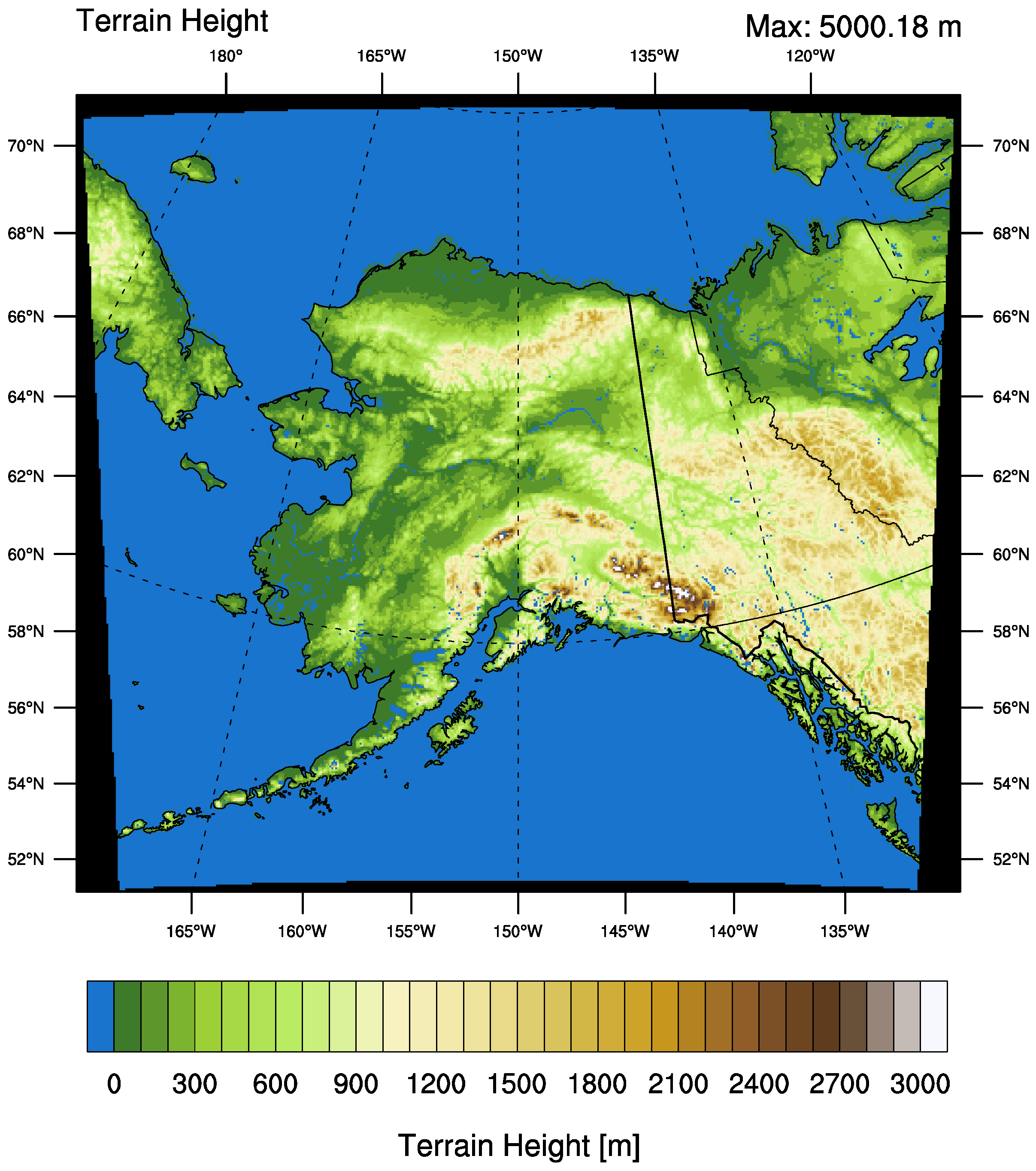
The WRF computational domain (Figure 1) covers all of Alaska and its territorial waters except for the western Aleutian Islands, due to computational cost and lack of population there. The horizontal grid spacing is 4 km. There are 49 vertical levels, seven of which are in the lowest kilometer, with a model top of 30 hPa. The European Centre for Medium-Range Weather Forecasting (ECMWF) Interim Reanalysis (ERA-Interim; [27]) was used to provide the initial and boundary conditions, as the ERA-Interim has been shown to perform well in Arctic regions [28]. Version 4.1 of the Multi-scale Ultra-high Resolution (MUR) sea surface temperature (SST) analysis [29] provided daily updates for SST and sea ice concentration at 0.01° grid spacing, which were resampled to 0.04° to approximately match the 4-km grid spacing of the WRF simulation. The lateral boundary conditions were updated every 6 h, and the lower boundary conditions were updated daily. The physics parameterizations are listed in Table 1.
The choice of ABL and surface layer parameterization scheme of course has an impact on near-surface and rotor-layer winds, as they each model atmospheric turbulence somewhat differently. This WRF simulation uses the Yonsei University (YSU) boundary layer scheme [32] and the MM5 similarity surface layer scheme [33,34], which follows Monin–Obukhov similarity theory [38,39]. The YSU ABL scheme is a non-local-K closure mixing scheme, and previous studies assessing several ABL schemes in WRF for wind speed and direction simulation have found that the YSU scheme performs best relative to other ABL schemes in unstable conditions, while YSU performs somewhat more poorly in stable conditions (e.g., [40,41]). The Draxl et al. [40] study compared seven ABL-surface layer schemes in WRF over a one-month period against observations up to 160 m AGL from a met mast and light tower in western Denmark. In contrast, Carvalho et al. [41] compared five ABL-surface layer schemes in WRF over a one-year period against surface observations: 13 onshore stations and five fixed offshore buoys in the Atlantic Ocean near Spain and Portugal. In both those studies, wind speed and direction from the YSU ABL scheme was generally middle-of-the-pack overall in terms of several standard error metrics, though it is recognized that the results may differ from region to region. It was beyond the scope of this study to perform a detailed comparison of several ABL schemes for the Alaska region, and we instead chose to leverage a 14-year high-resolution WRF simulation that had already been created for other applications. While it is possible that an ABL scheme other than YSU might have yielded reduced errors in the wind simulations in the Alaska region, the benefits gained from a 14-year numerical simulation are substantial. The primary purpose of this resource assessment study is to estimate the resource potential and indicate promising areas to target with in situ measurement campaigns and more detailed study for potential offshore wind farm development.
After spinning up the land surface state offline, the WRF simulation was initialized on 15 August 2002, and was run through 31 August 2016. After discarding the first two weeks of the simulation for hydrological system spin-up, the final WRF simulation dataset spans 1 September 2002–31 August 2016, a full 14-year period. Key variables, including 3-D temperature and wind fields, as well as 2-D near-surface fields and various hydrological and soil variables, were written out every hour and are publicly available for download and analysis [42].
2.2. Observations and Statistics for Validation
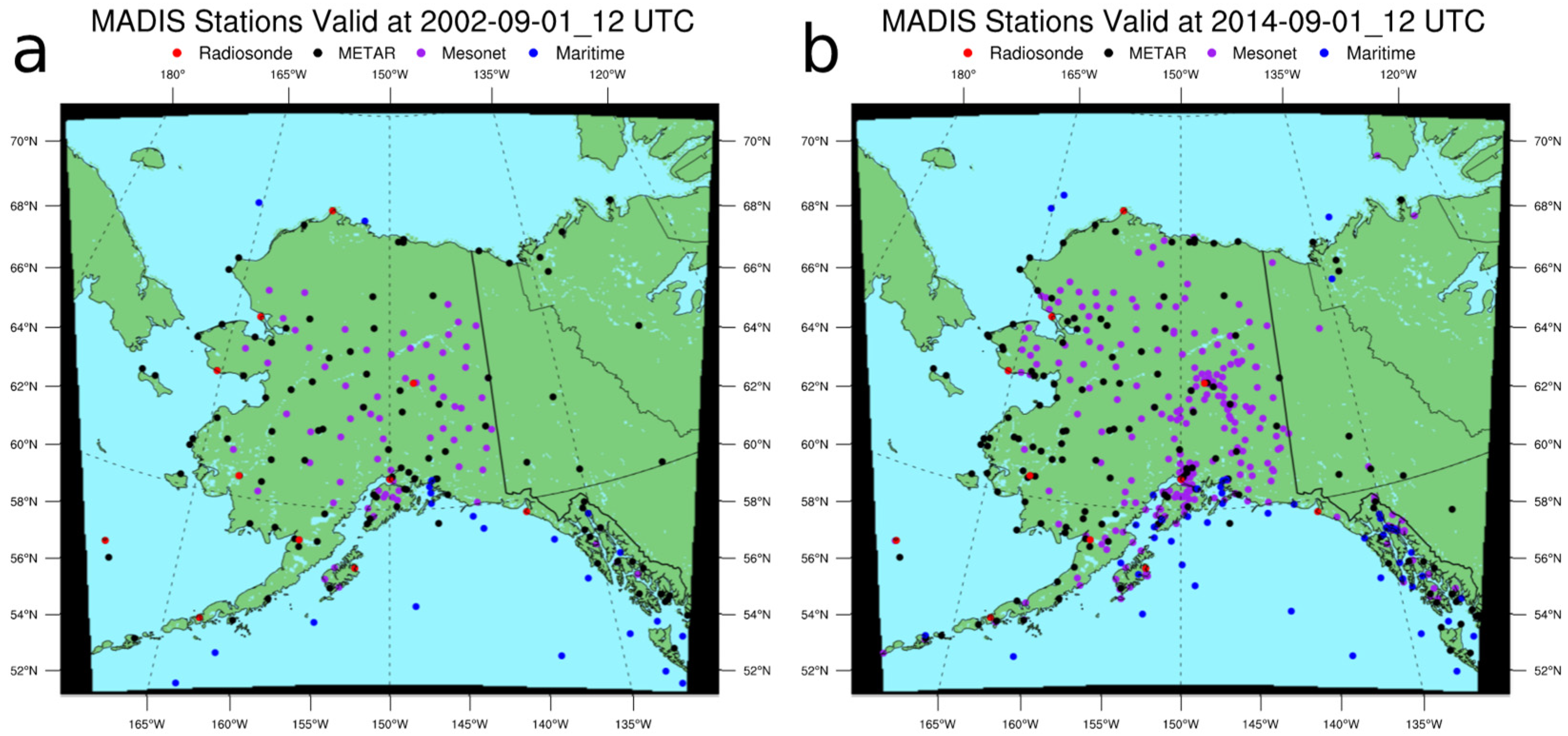
To validate the long-term WRF data set, we used wind speed observations from radiosondes from the lowest 500 m above ground level (AGL) within Alaska. As the primary focus of this work was to validate the model for areas offshore of Alaska, excluding radiosondes from outside Alaska has little impact on the final results. Including radiosonde observations up to 500 m AGL allows for a thorough validation of the WRF-simulated wind speed in the turbine rotor layer, though only onshore. Radiosondes were available twice daily, at 00 and 12 UTC. The locations of these radiosondes are indicated by red dots in Figure 2. While the number of radiosondes remained constant, the density of other observation types increased from 2002–2014, particularly for mesonets.
The metrics used to validate the WRF simulations are the standard metrics of root mean squared error (RMSE), mean absolute error (MAE), mean error (ME, or bias) that require no definition here, and also a skill score called the Nash–Sutcliffe efficiency (NSE). The NSE [43,44] is a normalized skill score to assess model performance. While the NSE has traditionally been used in hydrological applications, it can also be applied to any kind of model with paired observations of the same quantities. The NSE is defined as follows in Equation (1):
where is the total number of model/observation pairs being evaluated, is the th observed quantity, is the th modeled quantity, and is the mean of the observations. NSE is a positively oriented metric that ranges in value from to 1 (inclusive). A perfect score of indicates that the model perfectly matches the observations; indicates that the model is a better predictor of the quantity of interest (wind speed, in this study) than the mean of the observations; and indicates that the mean of the observations is a better predictor of the quantity of interest than the model.
All the metrics (RMSE, MAE, ME, and NSE) were calculated first on an hourly basis, then aggregated into daily average values, monthly average values, and annual average values. Observations from the various networks (radiosonde, METAR, mesonet, and maritime) were kept segregated to assess the relative quality of the networks themselves, especially in light of different observation heights (above-surface vs. surface-based) and other potentially systematic differences between networks (e.g., while the METAR wind speed observations can be safely assumed to be at 10 m AGL, the mesonet and maritime observations are likely less frequently at 10 m AGL). Furthermore, these statistics were calculated both domain-wide and for the specific energy regions individually, as defined in Section 2.3.
For the surface wind observations (METAR, mesonet, and maritime), WRF diagnostic 10-m wind speeds were interpolated horizontally from surrounding grid points using inverse distance weight interpolation. For radiosonde observations, WRF prognostic wind speeds were interpolated first horizontally to the radiosonde location using the same procedure, and then interpolated linearly in height to the observation heights. As we only included observations below 500 m AGL (i.e., mostly within the ABL) in our validation, this was deemed an acceptable approximation.
2.3. Defining Energy Regions
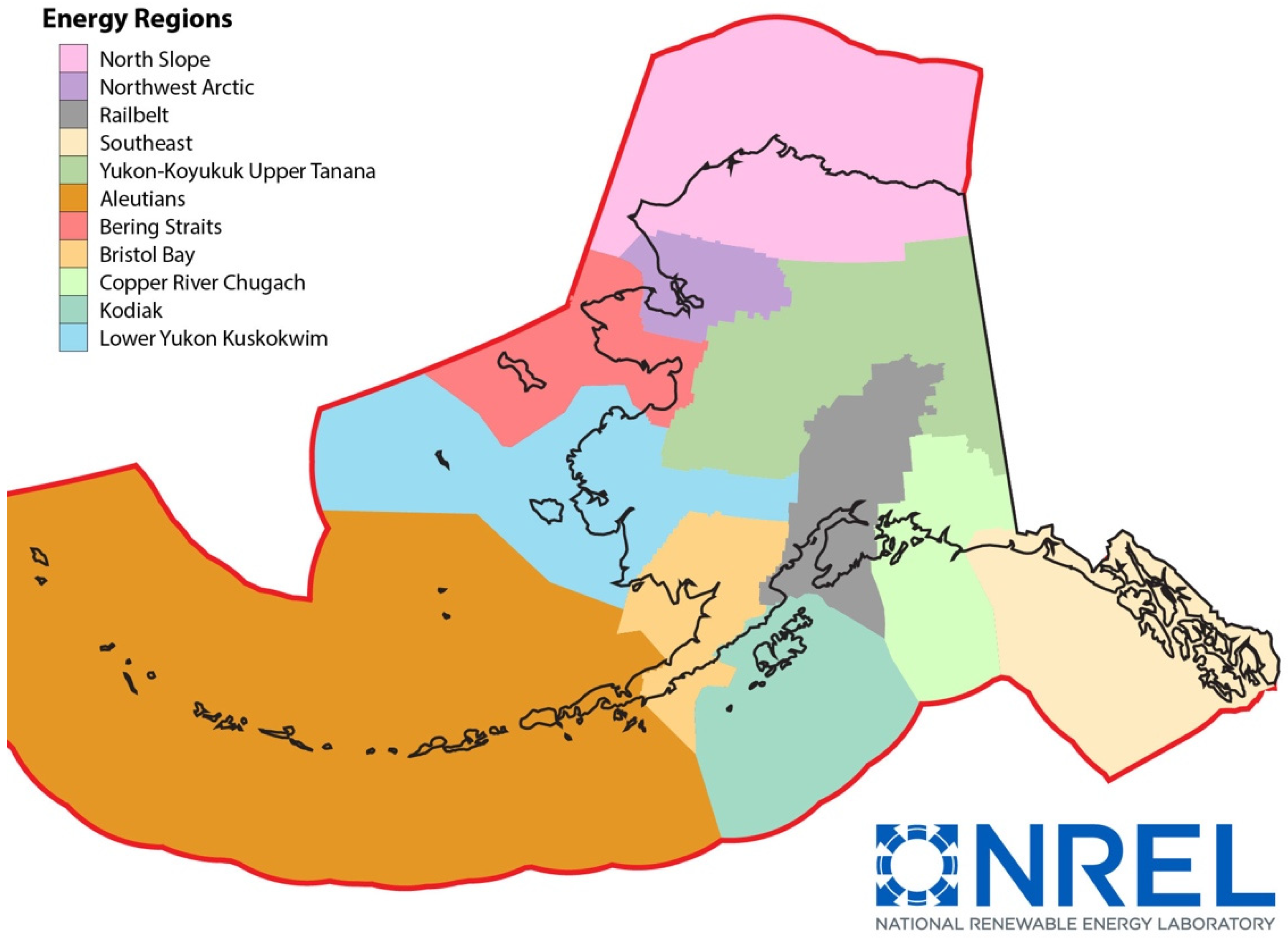
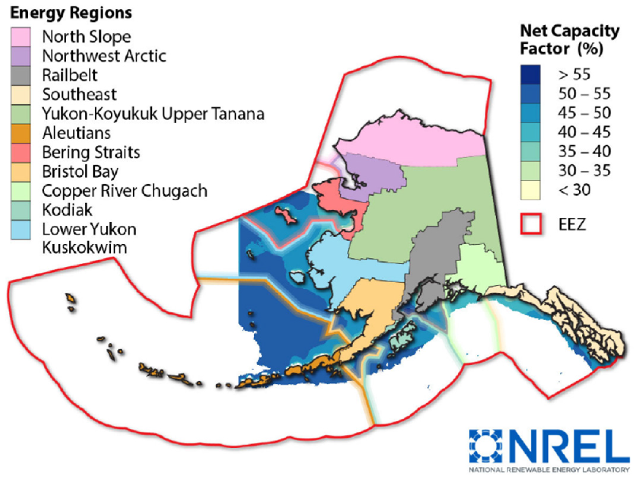
The Alaska Energy Authority (AEA) defined and parsed the state’s land area into 11 energy regions for the purpose of planning and energy diagnostics [45]. No such accepted definition existed for demarking offshore energy regions, however. Therefore, NREL, in [9], extended the AEA’s onshore energy regions out past the coastline to the exclusive economic zone (EEZ) limit by assigning each point to the closest onshore region, as shown in Figure 3. The EEZ is defined in the United Nations Convention on the Law of the Sea [46] as the sub-ocean area extending 200 nautical miles (370.4 km) outward from the coastline, except where limited by nearby states, provinces, or nations. If an area of water is within 200 nautical miles of two or more states/provinces/nations, then an agreement between those governments must be reached to establish the EEZ boundary.
3. Offshore Wind Resource Assessment
In this section, we present some of the key aspects of the wind resource assessment for Alaska’s offshore regions that are based on the aforementioned 14-year WRF dataset. The summary presented herein revisits the main results found in [9], an NREL Technical Report, to provide context for the wind data set validation that follows in Section 4. The information in this section has not previously been reported in the peer-reviewed journal literature, and is therefore novel.
The first step to a wind resource assessment is to define the area in which to conduct the assessment. Figure 3 illustrates the gross resource area under consideration, out to the EEZ limit. The technical resource area is a subset of the gross area, determined by various conditions in which offshore wind energy is expected to be technically feasible with current technology. Future innovation in the wind energy industry is expected to revise and expand the technical resource area. In addition to the western boundary of the WRF domain, the cutoffs to determine the technical resource area in this study were as follows:
- Bathymetry of 1000 m or less, as an approximate ocean depth limit provided by global developers of floating offshore wind technology.
- Latitude below 65.5° N, approximately the narrowest point of the Bering Strait, due to the prevalence of sea ice in climatological data [48].
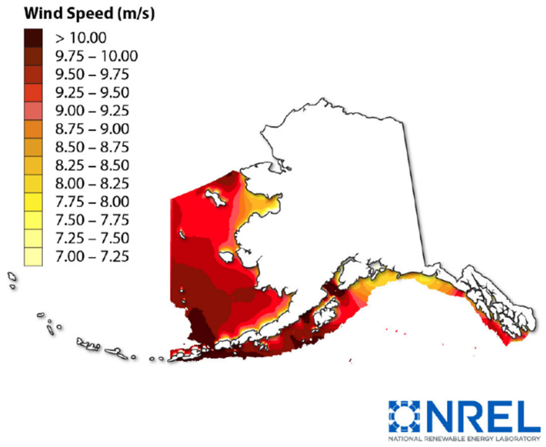
After applying these technical exclusions, the technical resource area within the WRF domain is 991,409 km2. It should be noted that this analysis did not account for environmental exclusions (e.g., marine sanctuaries) or other use exclusions (e.g., shipping lanes). A map of the technical resource area with the 14-year 100-m average wind speed from WRF is presented in Figure 4. The bulk of this technical resource area is in the Bering Sea, owing to its relatively shallow bathymetry. The Bering Sea also has some of the best wind resource, with widespread areas of average 100-m wind speeds in excess of 9 m s−1. Areas just south of the Aleutians also had high average wind speed. Perhaps the most prominent area with high wind speed in proximity to population centers and the Alaska Grid is an area of gap flow between Kodiak Island and the southeastern tip of the Kenai Peninsula, where average hub-height wind speeds exceed 10 m s−1. The slowest average hub-height wind speeds offshore were modeled in the Norton Sound south of Nome, along the northern edge of the Aleutians and Alaska Peninsula, and along the northern edge of the Gulf of Alaska. These regions of relatively weaker average wind speed are likely due to terrain shadowing.
By assuming a nominal wind power array density of 3 MW km−2, the technical offshore resource capacity in Alaskan waters is 2974 GW. By comparison, the technical offshore resource for CONUS and Hawai’i is 2658 GW [5]. After accounting for estimated potential wake, electrical, and other losses in developing an estimated net capacity factor (Figure 5; [9]), the technical resource net energy potential in Alaskan waters is 12,087 TWh y−1, which is a full 30% higher than the 9284 TWh y−1 of technical offshore resource energy potential from all other states combined [5], thus highlighting the tremendous potential for recoverable wind resource in Alaskan waters.
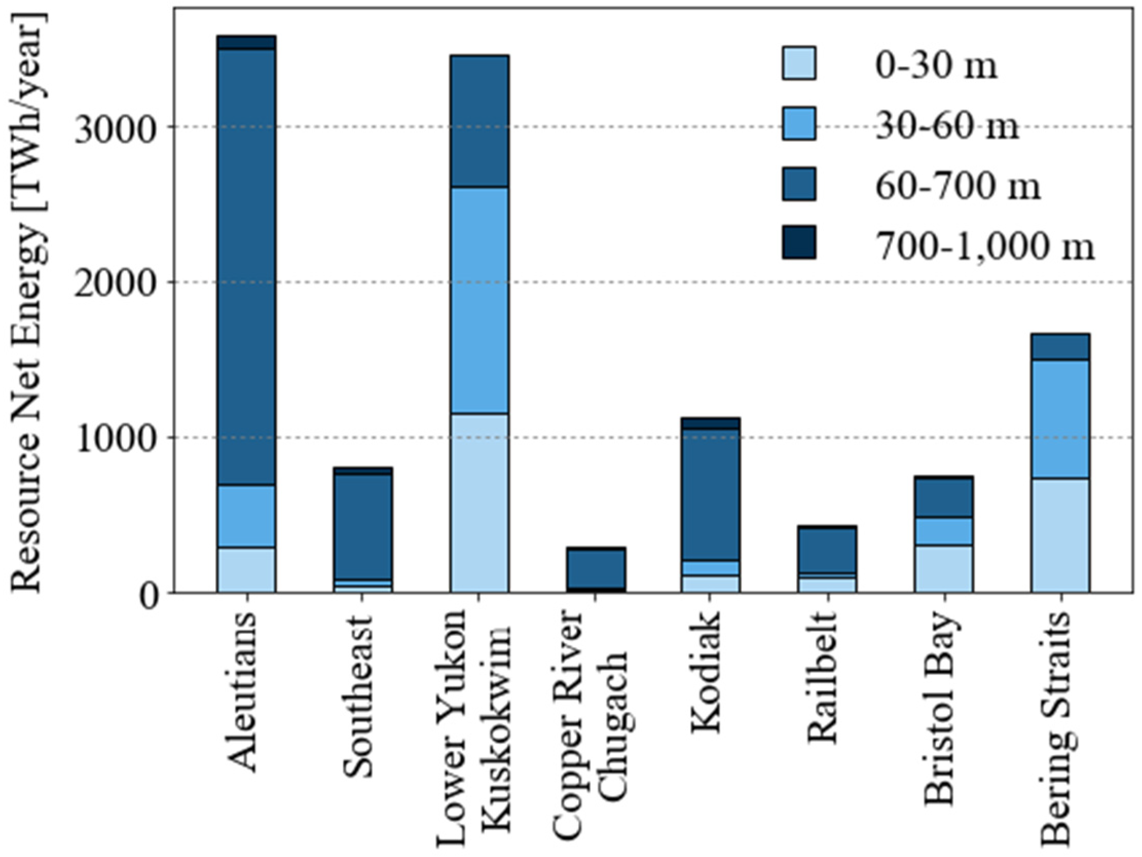
Breaking down the technical offshore net energy potential by region and by water depth, all regions except for Southeast and Copper River Chugach have at least 100 TWh y−1 in net energy potential in the shallowest waters, 0–30 m (Figure 6). Even these shallow-water energy potential figures dwarf the total electric generation in Alaska of 6.3 TWh in 2016 [49]. The bulk of the net energy potential in the Aleutians, Southeast, Copper River Chugach, Kodiak, and Railbelt regions is in the 60–700 m depth range, which exceeds the depth of current fixed-bottom turbine technological limits but which might potentially be recoverable with floating wind turbines.
4. Results
4.1. Domain-Wide Results
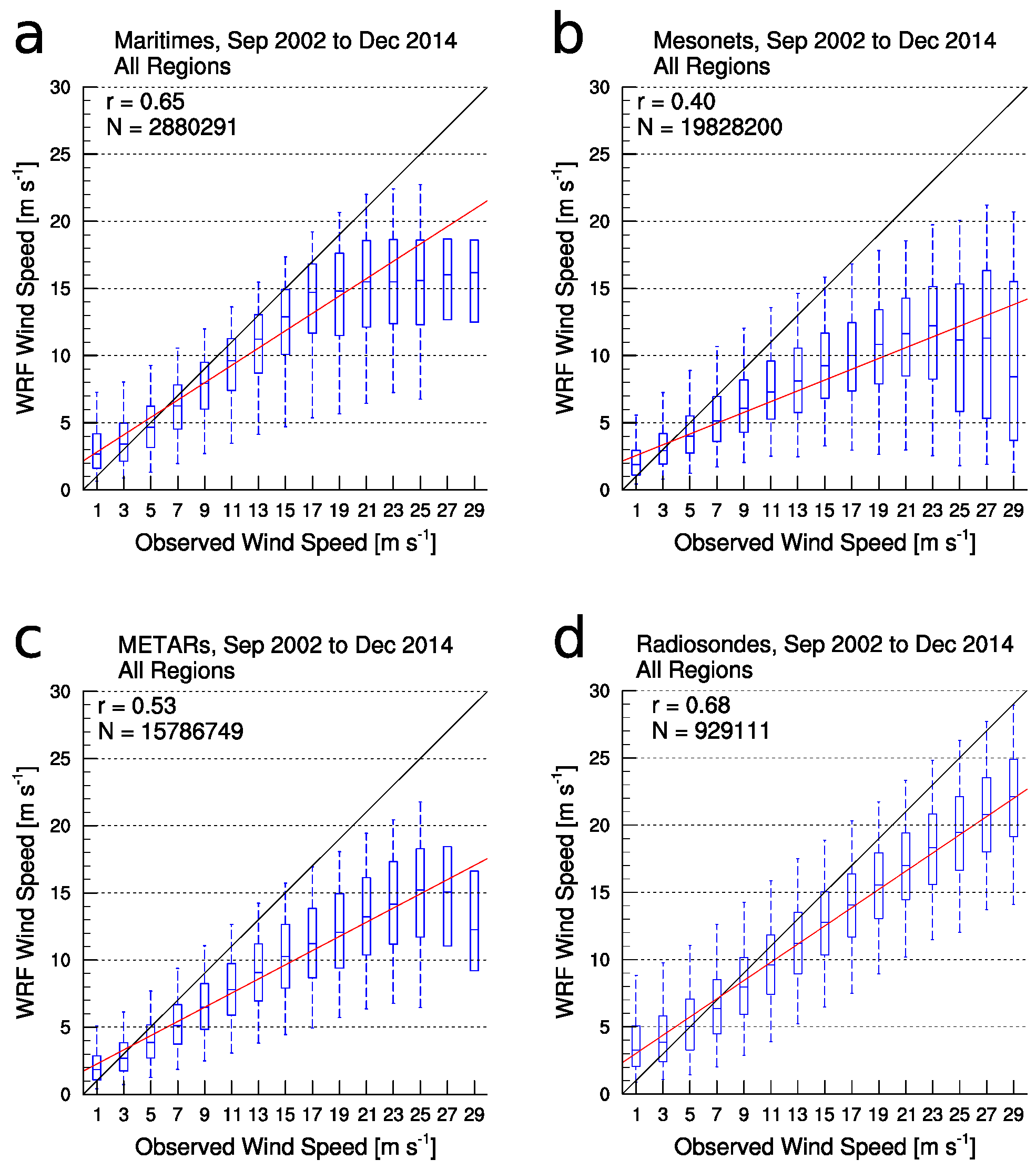
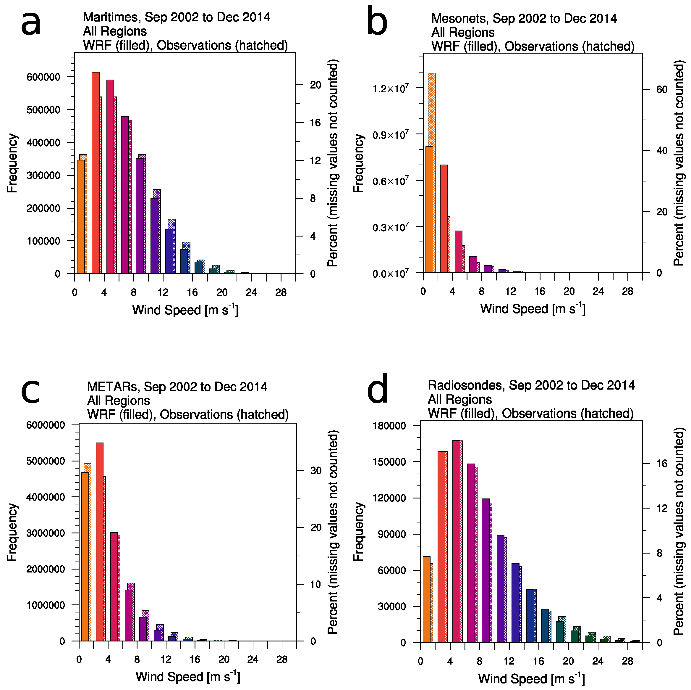
For validation of the WRF simulations, characteristics of the modeled and observed wind speed distributions across the entire domain are examined through box plots (Figure 7) and binned histograms (Figure 8). For both of these figures, the distributions are broken out by observation platform, with the maritime sites in panel (a), mesonets in panel (b), METARs in panel (c), and radiosondes in panel (d). Though our primary focus is on validating the WRF data set for offshore wind resource assessment, it is still valuable to include validation results for the WRF simulations over land, as an indication of the overall quality of the WRF simulations. For the box plots, the sample size N and regression coefficient r are also given; for example, there are 2.88 million model/observation pairs in the maritime network (Figure 7a), with a regression coefficient r = 0.65 and with a lot of scatter. For radiosondes (Figure 7d), the regression coefficient is similar (r = 0.68), also indicating moderate agreement between WRF and the observations for wind in the lowest 500 m AGL. Interestingly, from all four panels, it is apparent that this WRF regional climate dataset tends to overpredict low wind speeds and underpredict moderate and high wind speeds in an average sense over the entire domain. The level of agreement between the model and observations both over water (at the surface) and in the wind turbine rotor layer (over land) indicates that this WRF dataset is useful for offshore wind resource assessment, at least for providing a broad perspective for the general regions that could merit further investigation with more detailed assessment and targeted validation efforts. Conversely, the regression coefficient at mesonet sites (Figure 7b) is low (r = 0.40).
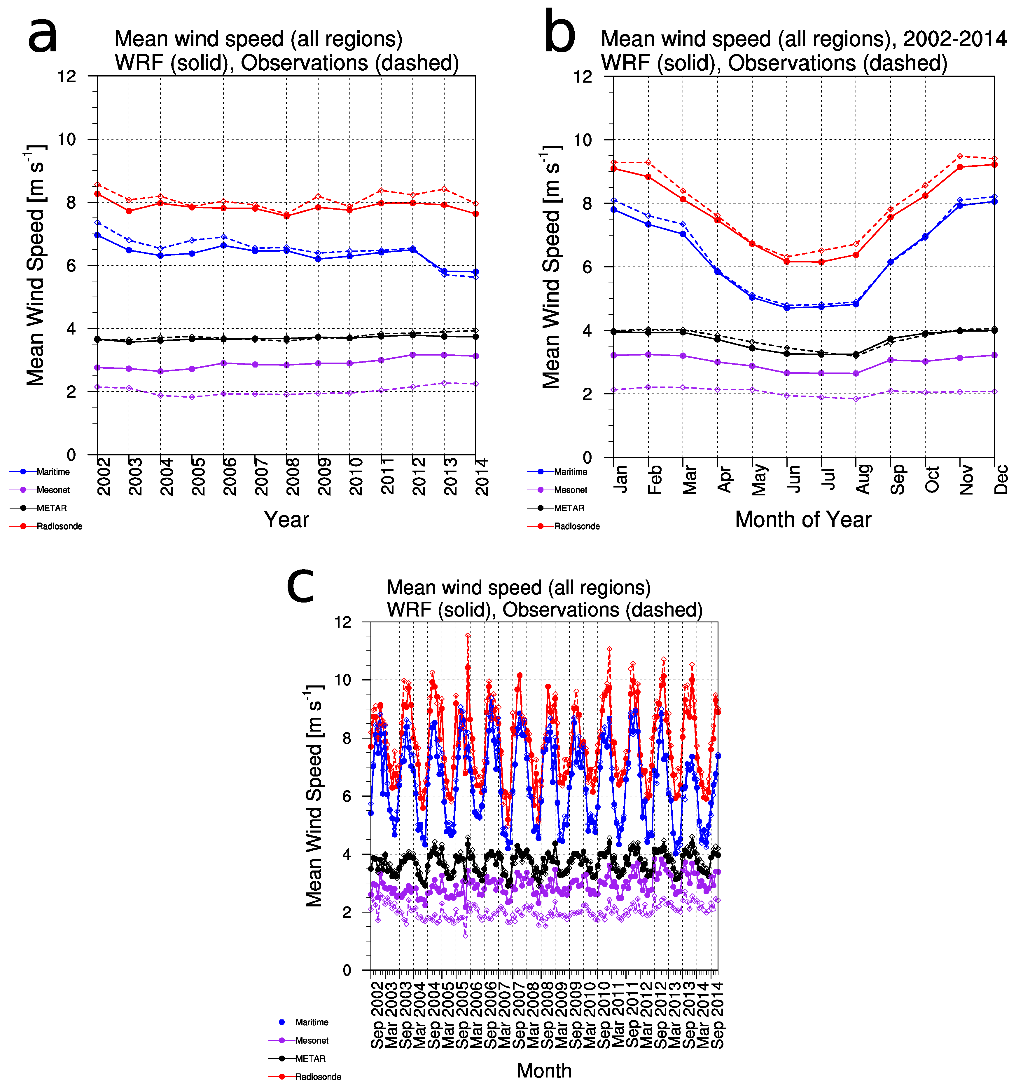
The information from the box plots and binned histograms are also consistent with plots of the domain-wide mean wind speed from WRF and the observations through time (Figure 9). The mean wind speed is averaged (a) on an annual basis, (b) on an annual cycle (month-of-year) basis, and (c) on a monthly basis. Averaging the data in these three ways yields complementary information.
First, from all three panels of Figure 9, we see that for maritime (blue), METAR (black), and radiosonde (red) stations, the WRF generally slightly underpredicts the observations in nearly every averaging interval. For mesonet (purple) stations, however, the WRF modeled wind speed is consistently higher than the observations by roughly 1 m s−1 in nearly every averaging interval. This overprediction of the wind speed by WRF is entirely consistent with the binned histograms in Figure 8b, where the WRF wind speed bins are higher than the observed wind speed bins for every wind speed above 2.0 m s−1.
Second, the wind speed across all networks is generally consistent from year to year (Figure 9a), both in the modeled and observed wind speed. Annual average observed wind speed for the radiosondes is about 8 m s−1, while for maritime stations it ranges generally from 6–7 m s−1. Observed wind speeds at the METAR stations are just below 4 m s−1, while for mesonet stations they are just 2 m s−1 on average. This plot shows that the inter-annual variability of both modeled and observed mean wind speed across this modeling domain is low throughout the period of 2002–2014, even when various large-scale climate signals like the Pacific Decadal Oscillation and El Niño–Southern Oscillation changed signs and amplitudes. Low inter-annual variability of wind speed inherently reduces uncertainty in estimates of wind power capacity factor and energy potential.
Third, there is a clear annual cycle in the radiosonde and maritime winds (Figure 9b), with average observed wind speeds typically about 3 m s−1 higher in winter months than in summer months. An annual cycle with stronger winds in winter than summer is expected from synoptic patterns, especially where surface friction has less impact (i.e., above the surface and over open water). For METAR stations the magnitude of the annual cycle is only about 1 m s−1, while for mesonet stations an annual cycle is barely discernible. This annual cycle is also borne out in the monthly average plot of mean wind speed (Figure 9c). For brevity, plots in the remainder of the paper only show annual average and annual cycle statistics, not monthly average.
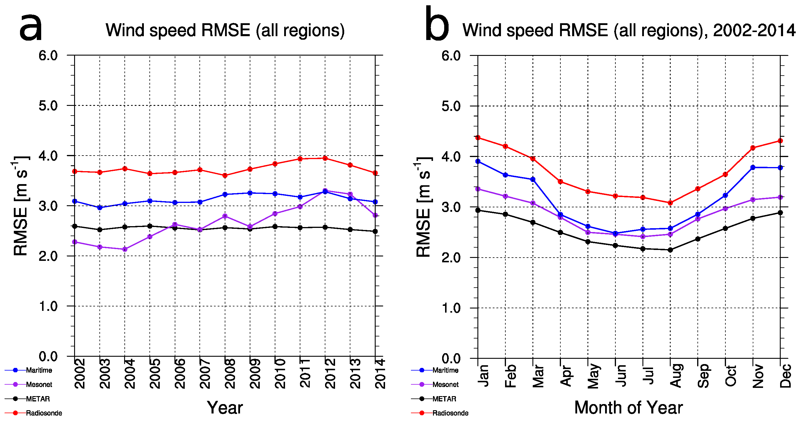
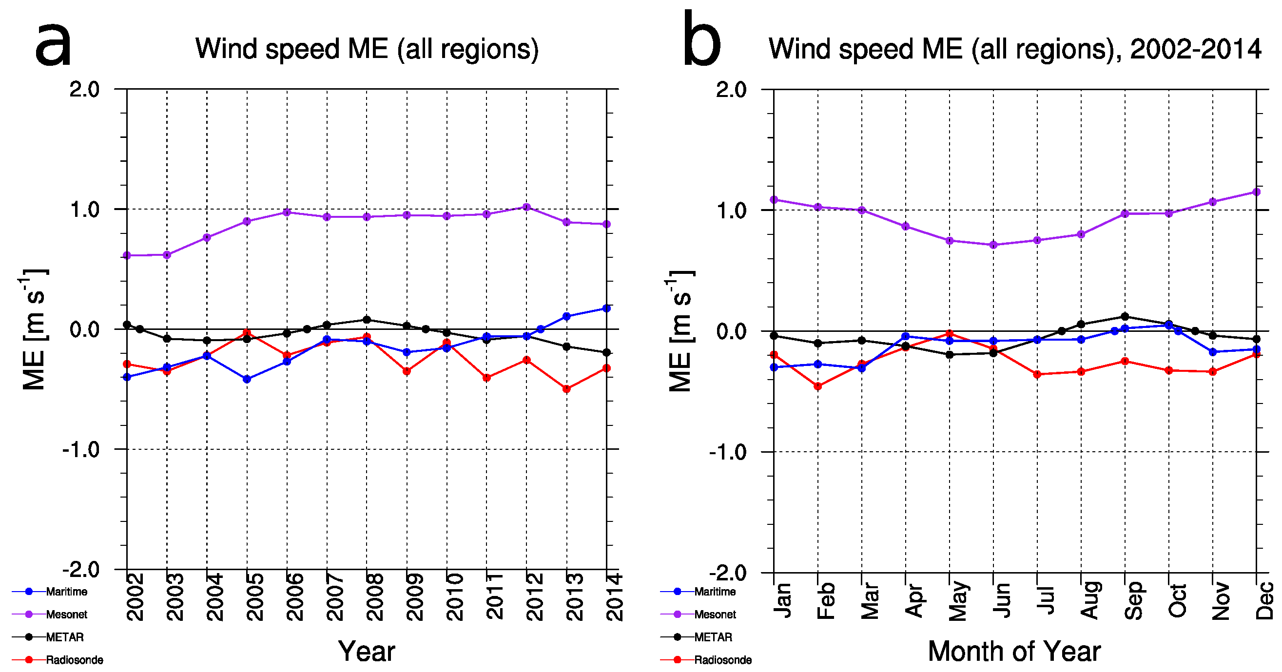
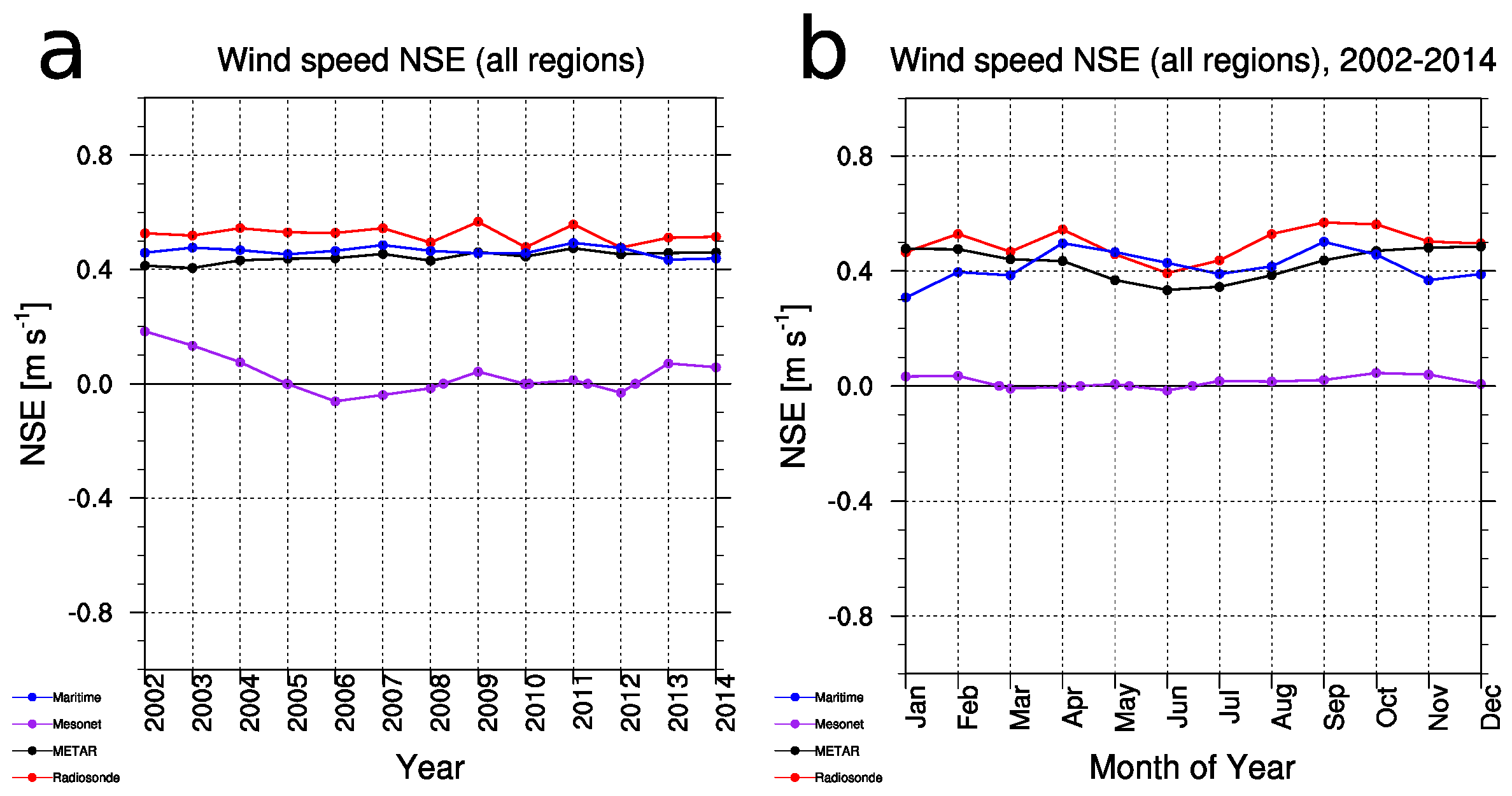
The domain-wide annual average and annual cycle values of error statistics are displayed in Figure 10 (RMSE), Figure 11 (ME), and Figure 12 (NSE). MAE figures are not shown for brevity.
The same annual cycle that was apparent in the mean wind speed (Figure 9b,c) is also apparent in the graphs of RMSE (Figure 10b), though an annual cycle is less apparent for either ME (Figure 11b) or NSE (Figure 12b). For the maritime observations, the RMSE ranges from about 2.5 m s−1 in summer to about 3.9 m s−1 in winter (compared to observations of about 4.9 m s−1 and 8.0 m s−1 in summer and winter, respectively), averaging from 3.0–3.3 m s−1 annually (Figure 10a). The MAE for maritime wind speed observations average from 2.2–2.5 m s−1 annually (not shown).
The ME plots make it even more apparent than the mean wind speed plots that the WRF simulations are nearly unbiased for the maritime, METAR, and radiosonde stations, both when looking at the annual average (Figure 11a) and the average annual cycle (Figure 11b). WRF has a small but consistent positive bias of about 0.6–1.2 m s−1 in every month for mesonet observations, however, which is consistent with previous results mentioned above. A likely explanation of this positive wind speed bias is that the mesonet wind speed observations are likely mostly taken at a lower height than 10 m AGL, unlike the METAR wind speed observations. (The MADIS data files do not contain metadata about reporting height, which is why mesonet observations in this study were assumed to be at 10 m AGL, like the METARs.) Because wind speeds generally decrease with decreasing height in the atmospheric boundary layer due to surface friction, wind speed observations from a lower reporting height (e.g., 3 m AGL) would be slower on average than a higher reporting height (10 m AGL). Thus, validating these observations against 10 m wind speeds from WRF would be expected to result in a positive bias for the model. This explanation is also consistent with the 2002–2014 observed average wind speed at mesonet stations being consistently about 2 m s−1 lower than at METAR stations (Figure 9).
The NSE (Figure 12) indicates positive scores, and therefore positive skill, domain-wide for the WRF simulations on an annual average basis and for the average annual cycle, when validated against radiosonde, METAR, and maritime observed wind speeds. These NSE values indicate that the WRF data set is a more skillful predictor than the mean of the observations for these observational networks. This is an important finding to highlight the utility and validity of this 14-year WRF dataset for wind resource assessment purposes, both onshore and offshore. For the mesonet observations, however, the NSE showed that WRF had little to no skill as a predictor compared to the mean of the observations. This finding is likely also explained by the uncertain reporting height of mesonet observations, as discussed in the preceding paragraph.
4.2. Regional Results
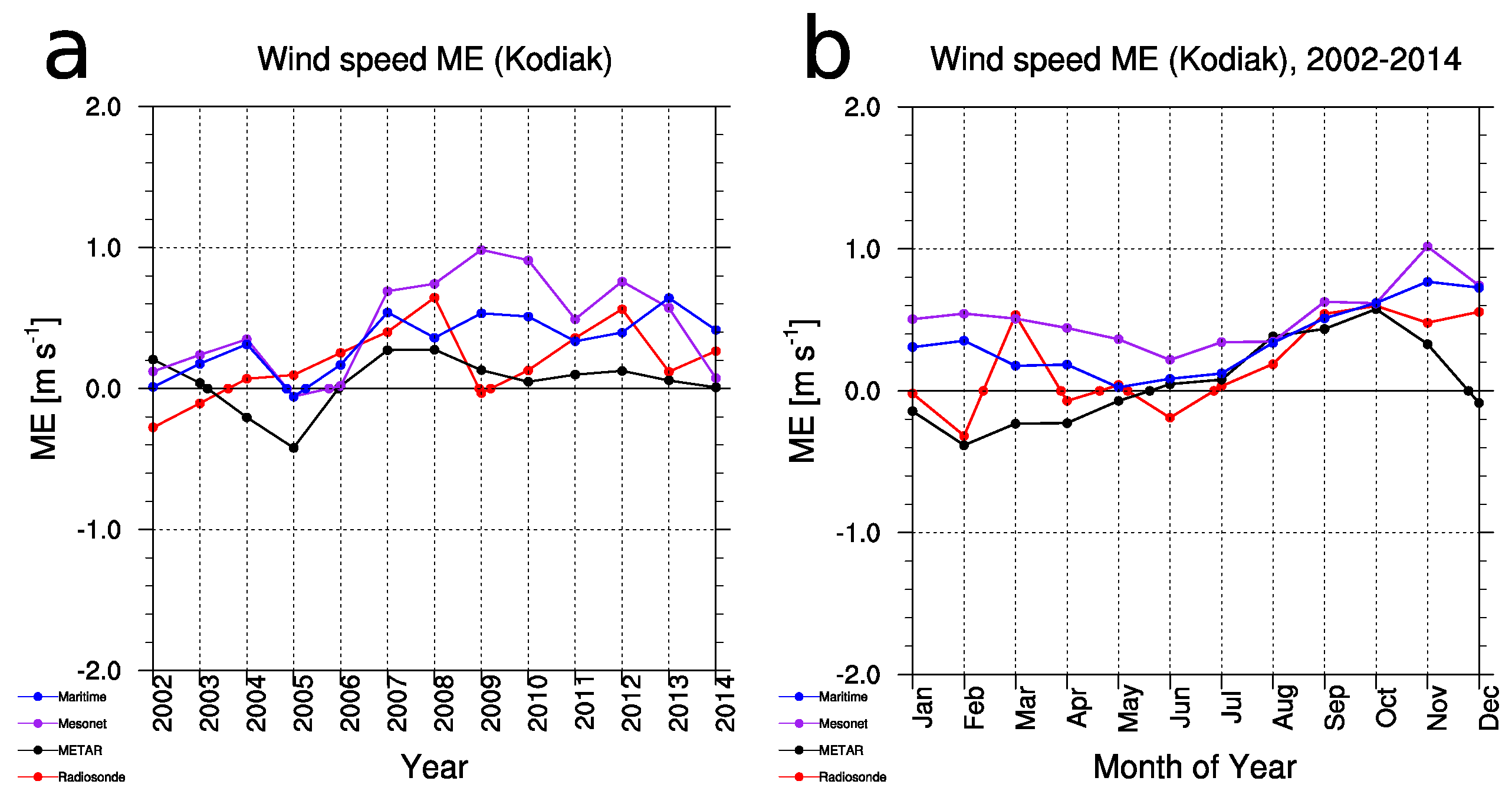
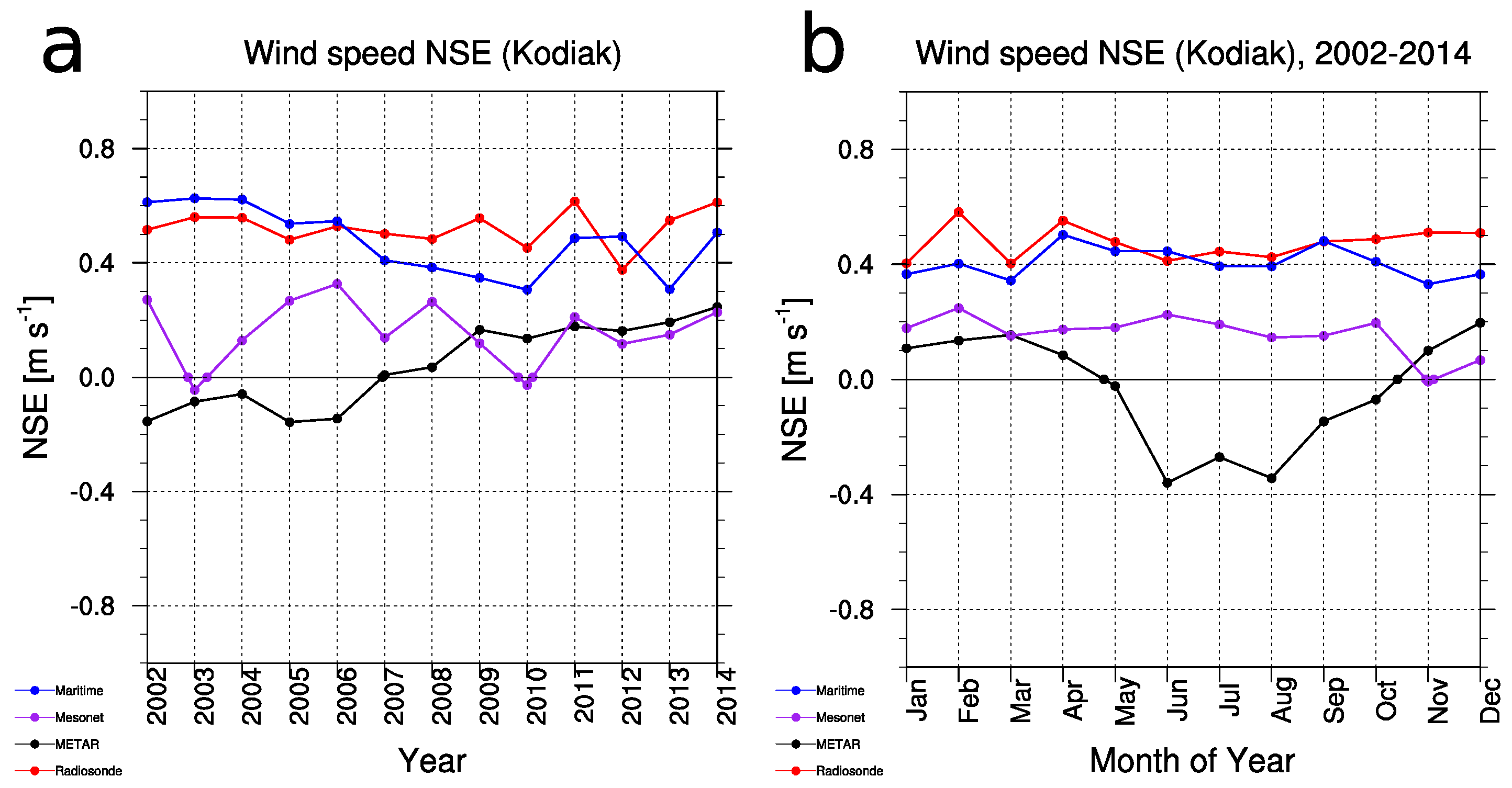
In addition to the domain-wide metrics and statistics presented in Section 4.1, it is useful to examine the same metrics within individual energy regions (Figure 3). Small sample sizes, due to few and/or infrequent observations being reported in a given region, complicate the analysis, however. Each of the statistics become noisier when validating a single region, and regional characteristics that differ from domain-wide average characteristics can also potentially emerge. As an example of the regional results, the Kodiak region is examined here. Box plots and binned histograms are displayed in Figure 13 and Figure 14. The mean wind speeds for the Kodiak region are shown in Figure 15. Figure 16 and Figure 17 show the RMSE and ME for the Kodiak region, as annual averages (panel a) and average annual cycles (panel b). The NSE for Kodiak is displayed in Figure 18. The same statistics for other regions are available in the Supplementary Materials to this article.
Perhaps the most obvious difference between the statistics for the Kodiak region and the statistics for the entire domain is that the regional statistics are substantially noisier due to a much smaller sample size (see Figure 2 for two snapshots of observation distributions, which changed over time). In fact, Kodiak is one of the most well-sampled regions by maritime network observations; all but two other regions have fewer and/or more infrequent maritime observations reported, and so the statistics for those regions are even noisier than for Kodiak (see Supplementary Materials).
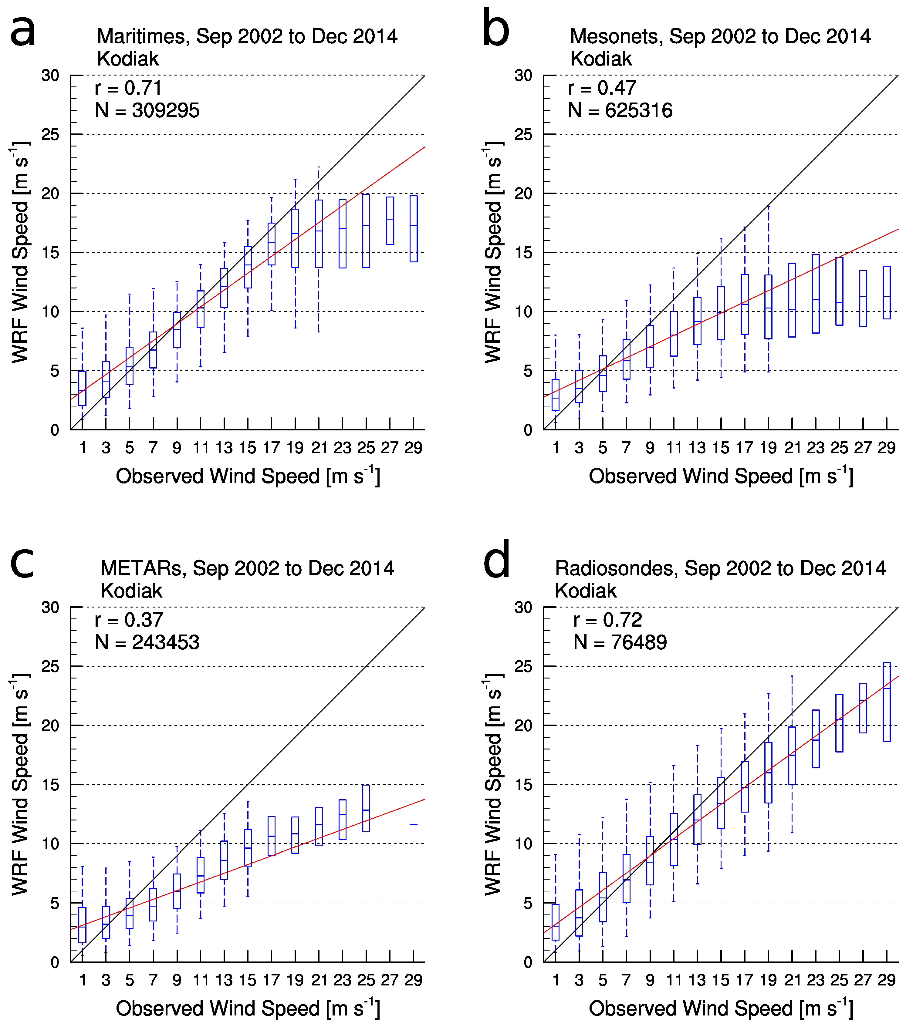
The box plots for the Kodiak region (Figure 13) are generally similar to the box plots for the whole domain (Figure 7), though the regression coefficient for the maritime, mesonet, and radiosonde networks is higher in Kodiak than in the domain as a whole, indicating better model agreement with observations in this particular region over the ocean near the surface and in the rotor layer over land.
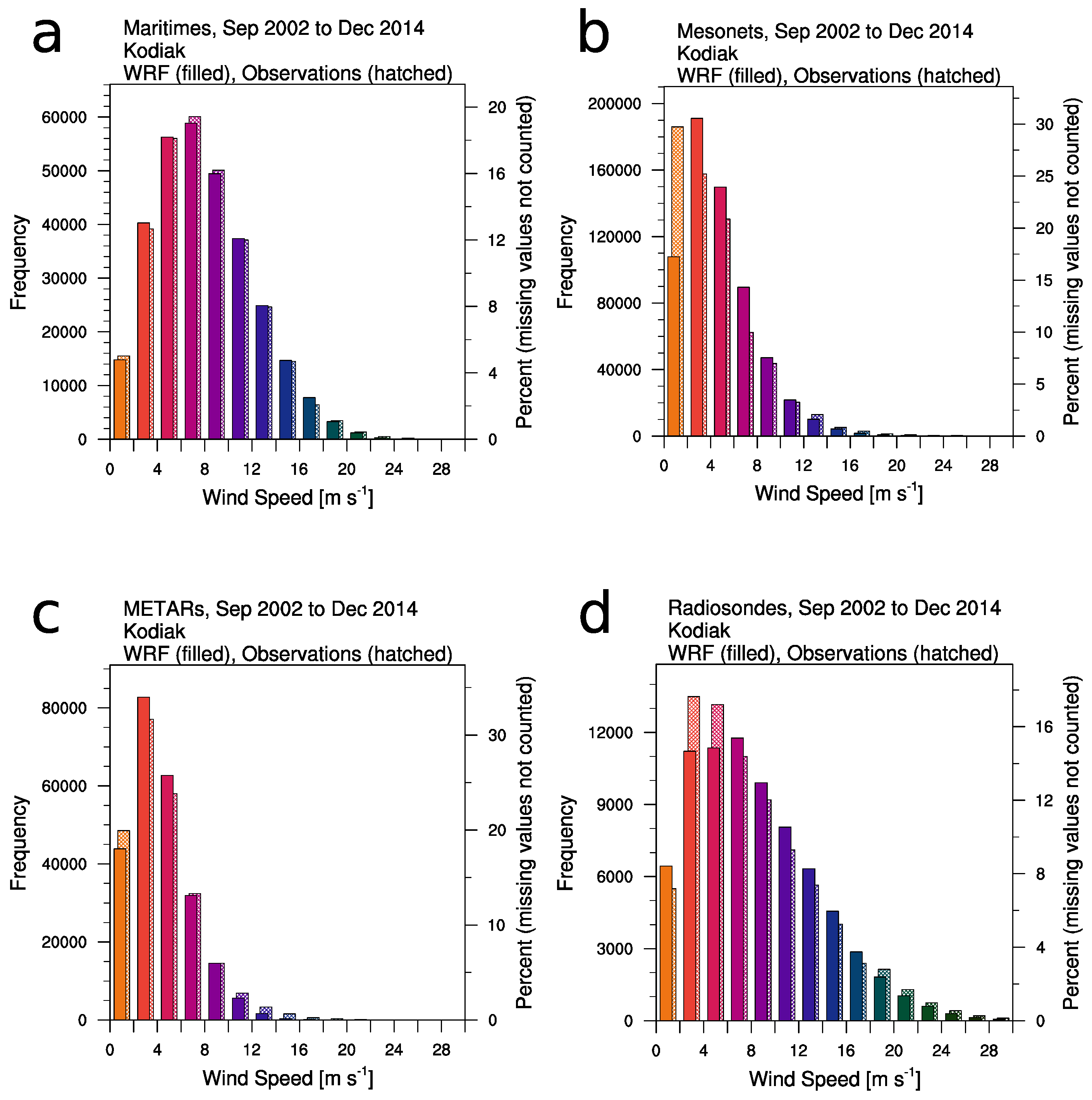
The binned histograms for the Kodiak region (Figure 14) are also somewhat similar to the histograms for the entire domain (Figure 8), though there are some small differences between them. The distributions of the modeled and observed wind speed for the maritime network in Kodiak (Figure 14a) are closely aligned, more so than in the domain as a whole. The distributions for the radiosonde network in Kodiak (Figure 14d) are less well aligned than in the domain as a whole, however, with the model clearly underpredicting the occurrence of wind speeds between 2–6 m s−1 and above 18 m s−1, while slightly overpredicting the occurrence of all other wind speeds.
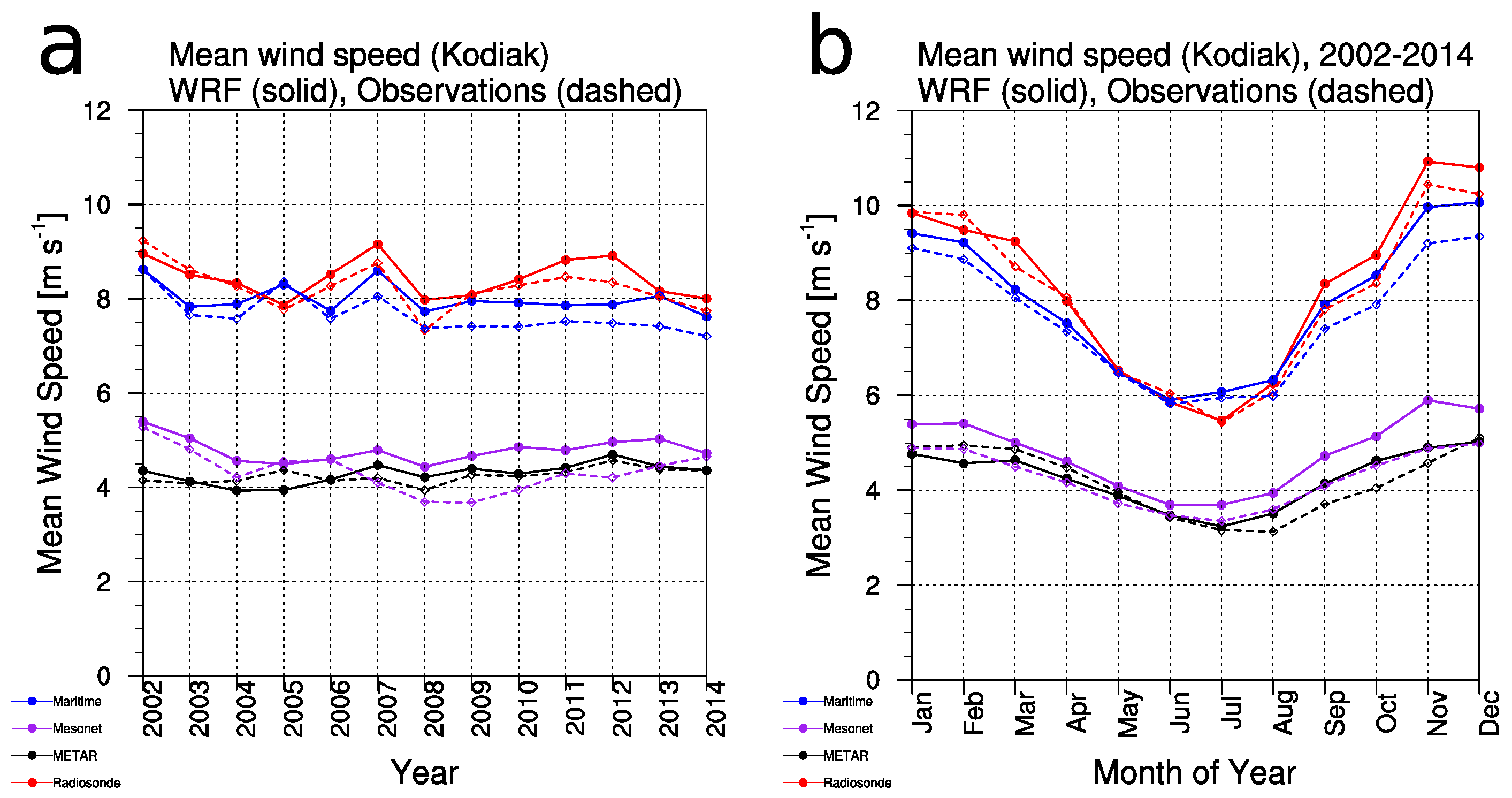
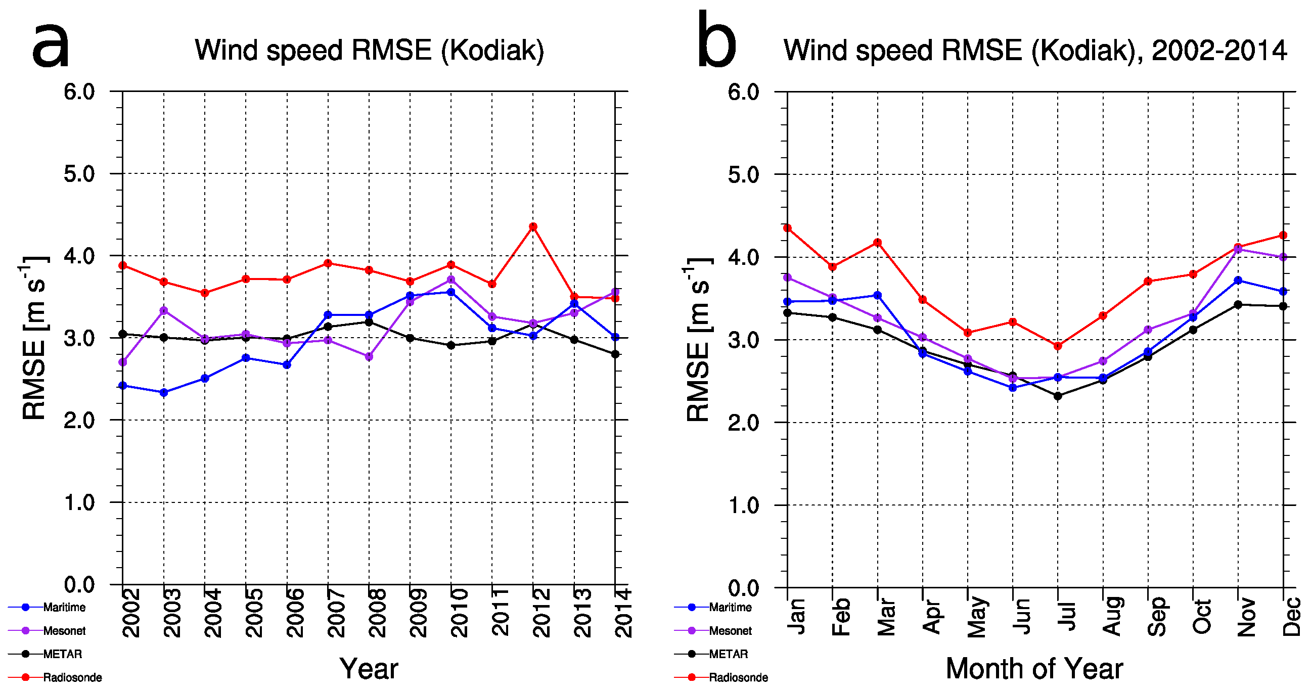
Noisier signals aside, the regional validation statistics tell similar stories to the domain-wide statistics. The annual cycle is still present, with maritime observed surface winds typically averaging 9–10 m s−1 during winter months and 6.0–6.5 m s−1 during summer months (Figure 15b). Monthly average RMSE for maritime wind speeds in Kodiak ranged from 2.5–3.5 m s−1 over the average annual cycle in the 2002–2014 record (Figure 16b). The WRF simulations also generally had a small (<1 m s−1) monthly average bias in most months, though that signal was somewhat noisy due to a relatively small sample size (Figure 17b). As in the domain-wide NSE, the regional NSE for Kodiak shows positive skill for WRF compared to the mean of the observations, both in an annual average sense and over an average annual cycle, for maritime and radiosonde observations (Figure 18). Interestingly, WRF displayed positive skill for the mesonet stations in this region, unlike for the domain as a whole, while skill for METAR stations was mixed, being negative early in the period and during summer and autumn months.
5. Discussion
Alaska, having only 2.7% (62 MW capacity) of its electricity generation coming from wind power, has a lot of room for growth in this sector, both onshore and offshore. Despite various challenges in the Alaskan environment, substantially increasing the penetration of wind power in Alaska will likely be necessary to increase total statewide generation from 29% renewables in 2016, both to meet aspirational statewide goals of 50% renewable generation by 2025 and more general goals of steadily decarbonizing the nation’s electric grid. The first step toward developing new wind farms is to assess the available wind resource. This study represents the first offshore wind resource assessment and validation for Alaska in the scientific literature and complements existing studies and data sets that assess the offshore wind energy resource for CONUS.
This offshore wind resource assessment was generated from a data set of publicly-available, 14-year, 4-km WRF regional climate simulations [26,42]. To our knowledge, no other published study for wind resource assessment uses such a long dataset of high-resolution NWP or regional climate simulations. Underpinning a wind resource assessment with such a lengthy dataset increases the robustness of the results and allows for better capturing of inter-annual variability.
From this 14-year WRF data set, the technical offshore wind energy resource capacity in Alaskan waters is 2974 GW with technical net energy potential of 12,087 TWh y−1. These numbers dwarf Alaska’s current annual electrical generation of 6.3 TWh and nearly quadruple current total U.S. annual electrical generation of 4077 TWh in 2016 [50]. This resource assessment identified broad areas of low bathymetry and high wind speed in the Bering Sea and south of the Aleutian Islands and Alaska Peninsula, but also small areas of the same in the Railbelt region between the Kenai Peninsula and Kodiak Island, with 14-year average modeled 100 m wind speeds in excess of 10 m s−1. Being close to population centers and the existing Alaska Grid transmission lines, this may be a natural first region to target with more high-resolution siting studies. In the shallowest waters (<60 m depth) in the Railbelt region alone, which could support bottom-anchored turbines, there is still over 100 TWh y−1 of net energy potential. The Southeast region is another area that could merit further studies, as it has a reasonably large energy potential while also being close to the BC Hydro grid that services British Columbia and southeast Alaska.
To determine the accuracy and skill of the 14-year WRF dataset, it was validated against radiosonde observations over Alaska (the lowest 500 m AGL) and against surface observations from MADIS (METAR, mesonet, and maritime networks). Despite the caveat of not having tall towers or offshore radiosondes against which to validate hub-height offshore winds, the surface wind and land-based radiosondes still allow a reasonable validation of the WRF model simulations of wind speed over a long period. We believe this study and high-resolution WRF regional climate dataset can serve as a general guide to indicate some potentially promising areas near Alaska for more detailed follow-up study and site assessment, including targeted observation and validation of wind speed offshore in the rotor layer.
Validating the simulations across the whole modeling domain against the radiosonde, METAR, and maritime observations resulted in near-zero average bias (−0.4–0.2 m s−1), both in a monthly average and annual average sense. These networks also generally had positive NSE scores, meaning that WRF was a better predictor than the observed mean, on average. The monthly averaged observations themselves, as well as the RMSE, all showed a distinct annual cycle with higher values in winter and lower values in summer. Validating against radiosondes showed an annual average RMSE of approximately 3.5 m s−1 over land in the lowest 500 m compared to an annual average RMSE of approximately 3.0 m s−1 when validating against maritime observations; the annual observed mean wind speed by radiosondes was approximately 7.5–8.0 m s−1, and the annual observed mean for 10-m maritime winds was approximately 6.0–7.0 m s−1 most years, domain-wide. The consistently positive ~+1.0 m s−1 bias and negative NSE of the modeled wind speed validated against mesonet observations serves as a likely indication that most of the mesonet observations were at a height below 10 m AGL, thus harming model skill.
Issues of small sample size dominated the regional validation and resulted in noisy statistics. This was particularly true for maritime observations in the smallest regions and in the regions further north in the Bering Sea, where fewer ships travel and report valid observations. For offshore wind validation, against observations from ships and buoys assumed to measure wind speed at 10 m AGL for this study in order to leverage model output (even though many buoy observations do have lower reporting heights), the lowest RMSE and near-zero bias was found in the Aleutians, Kodiak, and Southeast regions (Supplementary Materials). This was likely due to a combination of a greater number of observations in these regions than in others, and also fewer terrain impacts over the region as a whole.
6. Conclusions
In conclusion, this publicly available 14-year WRF regional climate simulation is skillful and suitable for use for both hydrometeorological and wind energy resource assessment applications. This validated data set has shown that Alaska has a tremendous offshore wind resource that is technically recoverable and can help inform decisions regarding potential development of offshore wind energy near Alaska’s vast coastline. Additional analysis is required, however, to further refine the technically recoverable wind resource, by accounting for environmental and other use exclusions, as well as accounting for specific technologies built to survive the cold, harsh climate. Assessment of the economic viability of specific sites for offshore wind development and build-out of transmission lines is beyond the scope of this work, however, but given the high electricity prices in much of rural Alaska, offshore wind power could prove to be an attractive option to meet a sizable portion of Alaska’s energy needs in future decades.
Supplementary Materials
Author Contributions
Conceptualization, L.X., P.D., and C.D.; Methodology, L.X., J.A.L., P.D., and A.J.N.; Software, J.A.L., P.D., A.J.N., and G.S.; Validation, J.A.L. and P.D.; Formal analysis, J.A.L.; Investigation, J.A.L.; Resources, L.X., P.D., and C.D.; Data curation, A.J.N., G.S., and P.D.; Writing—original draft preparation, J.A.L.; Writing—review and editing, J.A.L., P.D., L.X., A.J.N., C.D., and G.S.; Visualization, J.A.L., G.S., and P.D.; Supervision, L.X., P.D., and C.D.; Project administration, L.X. and C.D.; Funding acquisition, L.X. and C.D.
Funding
The Alliance for Sustainable Energy, LLC (Alliance) is the manager and operator of the National Renewable Energy Laboratory (NREL). NREL is a national laboratory of the U.S. Department of Energy (DOE), Office of Energy Efficiency and Renewable Energy. This work was authored by the Alliance and supported by the DOE under contract no. DE-AC36-08GO28308. Funding was provided by the DOE Office of Energy Efficiency and Renewable Energy and the DOE Renewable Energy, Wind and Water Power Technologies Office. The views expressed in this article do not necessarily represent the views of the U.S. Department of Energy or the U.S. government. The U.S. government retains, and the publisher, by accepting the article for publication, acknowledges that the U.S. government retains a nonexclusive, paid-up, irrevocable, worldwide license to publish or reproduce the published form of this work, or allow others to do so, for U.S. government purposes. Authors Lee, Xue, and Newman were supported by subcontract AHA-7-70142-01 from NREL to NCAR.
Acknowledgments
This material is based upon work supported by the National Center for Atmospheric Research, which is a major facility sponsored by the National Science Foundation under Cooperative Agreement No. 1852977. We would like to acknowledge high-performance computing support from Cheyenne [51] provided by NCAR’s Computational and Information Systems Laboratory (CISL). Several of the figures were created using the NCAR Command Language (NCL) [52]. We also thank Billy Roberts of NREL for designing some of the figures, as well as Mary Lukkonen and Sheri Anstedt of NREL for technical editing that improved the manuscript. Comments from two anonymous reviewers also improved the manuscript further.
Conflicts of Interest
The authors declare no conflict of interest. The funders had no role in the design of the study; in the collection, analyses, or interpretation of data; in the writing of the manuscript, or in the decision to publish the results.
References
- IEA. Wind Energy. International Energy Association, 2019. Available online: https://www.iea.org/topics/renewables/wind/ (accessed on 7 July 2019).
- AWEA. U.S. Wind Industry Annual Market Report, Year Ending 2016. American Wind Energy Association, 2017. Available online: https://www.awea.org/amr2016 (accessed on 2 March 2018).
- U.S. EIA. Wind Turbines Provide 8% of U.S. Generating Capacity, More than Any Other Renewable Source. Preliminary Monthly Electric Generator Inventory, U.S. Energy Information Administration. 2017. Available online: https://www.eia.gov/todayinenergy/detail.php?id=31032 (accessed on 2 March 2018).
- Deepwater Wind. America’s First Offshore Wind Farm Powers up. Press Release, Deepwater Wind. 2016. Available online: http://dwwind.com/press/americas-first-offshore-wind-farm-powers/ (accessed on 2 March 2018).
- Musial, W.; Heimiller, D.; Beiter, P.; Scott, G.; Draxl, C. 2016 Offshore Wind Energy Resource Assessment for the United States. National Renewable Energy Laboratory Tech. Report NREL/TP-5000-66599; p. 76. 2016. Available online: https://www.nrel.gov/docs/fy16osti/66599.pdf (accessed on 2 March 2018).
- U.S. EIA. Electric Power Monthly with Data for December 2017. U.S. Energy Information Administration, 2018. Available online: https://www.eia.gov/electricity/monthly/archive/february2018.pdf (accessed on 2 March 2018).
- Alaska State Legislature. Enrolled HB 306: Declaring a State Energy Policy. 2010. Available online: www.akleg.gov/basis/Bill/Text/26?Hsid=HB0306Z (accessed on 2 March 2018).
- Alaska Energy Authority. Alaska Energy Infrastructure: Pipelines and Electrical Lines. Dataset, Alaska Energy Data Inventory. 2010. Available online: https://en.openei.org/datasets/dataset/alaska-energy-infrastructure-pipelines-and-electrical-lines (accessed on 2 March 2018).
- Doubrawa, P.; Scott, G.; Musial, W.; Kilcher, L.; Draxl, C.; Lantz, E. Offshore Wind Energy Resource Assessment for Alaska. NREL Tech. Report NREL/TP-5000-70553; p. 29. 2017. Available online: https://www.nrel.gov/docs/fy18osti/70553.pdf (accessed on 2 March 2018).
- Lu, N.-Y.; Basu, S.; Manuel, L. On wind turbine loads during the evening transition period. Wind Energy 2019, in press. [Google Scholar] [CrossRef]
- Nandi, T.N.; Herrig, A.; Brasseur, J.G. Non-steady wind turbine response to daytime atmospheric turbulence. Philos. Trans. R. Soc. A 2017, 375, 20160103. [Google Scholar] [CrossRef] [PubMed]
- Churchfield, M.J.; Lee, S.; Michalakes, J.; Moriarty, P.J. A numerical study of the effects of atmospheric and wake turbulence on wind turbine dynamics. J. Turbul. 2012, 13, N14. [Google Scholar] [CrossRef]
- Salvação, N.; Guedes Soares, C. Resource assessment methods in the offshore wind energy sector. In Floating Offshore Wind Farms; Green Energy and Technology; Castro-Santos, L., Diaz-Casas, V., Eds.; Springer International Publishing: Cham, Switzerland, 2016. [Google Scholar] [CrossRef]
- Clifton, A.; Hodge, B.-M.; Draxl, C.; Badger, J.; Habte, A. Wind and solar resource data sets. WIREs Energy Environ. 2017, 7, e276. [Google Scholar] [CrossRef]
- Skamarock, W.C.; Klemp, J.B.; Dudhia, J.; Gill, D.O.; Barker, D.M.; Duda, M.G.; Huang, X.-Y.; Wang, W.; Powers, J.G. A Description of the Advanced Research WRF Version 3; NCAR Technical Note NCAR/TN-475+STR; National Center for Atmospheric Research: Boulder, CO, USA, 2008; p. 113. [Google Scholar] [CrossRef]
- Powers, J.G.; Klemp, J.B.; Skamarock, W.C.; Davis, C.A.; Dudhia, J.; Gill, D.O.; Coen, J.L.; Gochis, D.J.; Ahmadov, R.; Peckham, S.E.; et al. The weather research and forecasting model: Overview, system efforts, and future directions. Bull. Am. Meteorol. Soc. 2017, 98, 1717–1737. [Google Scholar] [CrossRef]
- AIAA. Guide for the Verification and Validation of Computational Fluid Dynamics Simulations [AIAA G-077-1998(2002)]; American Institute of Aeronautics and Astronautics: Reston, VA, USA, 1998. [Google Scholar] [CrossRef]
- Hahmann, A.N.; Vincent, C.L.; Peña, A.; Lange, J.; Hasager, C.B. Wind climate estimation using WRF model output: Method and model sensitivities over the sea. Int. J. Climatol. 2015, 35, 3422–3439. [Google Scholar] [CrossRef]
- Mattar, C.; Borvarán, D. Offshore wind power simulation by using WRF in the central coast of Chile. Renew. Energy 2016, 94, 22–31. [Google Scholar] [CrossRef]
- Chancham, C.; Waewsak, J.; Gagnon, Y. Offshore wind resource assessment and wind power plant optimization in the Gulf of Thailand. Energy 2017, 139, 706–731. [Google Scholar] [CrossRef]
- Salvação, N.; Guedes Soares, C. Wind resource assessment offshore the Atlantic Iberian coast with the WRF model. Energy 2018, 145, 276–287. [Google Scholar] [CrossRef]
- Draxl, C.; Clifton, A.; Hodge, B.-M.; McCaa, J. The Wind Integration National Dataset (WIND) Toolkit. Appl. Energy 2015, 151, 355–366. [Google Scholar] [CrossRef] [Green Version]
- James, E.P.; Benjamin, S.G.; Marquis, M. Offshore wind speed estimates from a high-resolution rapidly updating numerical weather prediction forecast dataset. Wind Energy 2018, 21, 264–284. [Google Scholar] [CrossRef]
- Benjamin, S.G.; Weygandt, S.S.; Brown, J.M.; Hu, M.; Alexander, C.R.; Smirnova, T.G.; Olson, J.B.; James, E.P.; Dowell, D.C.; Grell, G.A.; et al. A North American hourly assimilation and model forecast cycle: The rapid refresh. Mon. Weather Rev. 2016, 144, 1669–1694. [Google Scholar] [CrossRef]
- NREL, Alaska Wind 50-m Height. Dataset; 2009. Available online: www.nrel.gov/gis/data-wind.html (accessed on 2 March 2018).
- Monaghan, A.J.; Clark, M.P.; Barlage, M.P.; Newman, A.J.; Xue, L.; Arnold, J.R.; Rasmussen, R.M. High-resolution climate simulations over Alaska. J. Appl. Meteorol. Climatol. 2018, 57, 709–731. [Google Scholar] [CrossRef]
- Dee, D.P.; Uppala, S.M.; Simmons, A.J.; Berrisford, P.; Poli, P.; Kobayashi, S.; Andrae, U.; Balmaseda, M.A.; Balsamo, G.; Bauer, P.; et al. The ERA-Interim reanalysis: Configuration and performance of the data assimilation system. Q. J. R. Meteorol. Soc. 2011, 137, 553–597. [Google Scholar] [CrossRef]
- Lindsay, R.; Wensnahan, M.; Schweiger, A.; Zhang, J. Evaluation of seven different atmospheric reanalysis products in the Arctic. J. Clim. 2014, 27, 2588–2606. [Google Scholar] [CrossRef]
- NASA/JPL. GHRSST Level 4 MUR Global Foundation Sea Surface Temperature Analysis (v4.1); Physical Oceanography Distributed Active Archive Center: Pasadena, CA, USA, 2015. [Google Scholar] [CrossRef]
- Thompson, G.; Field, P.R.; Rasmussen, R.M.; Hall, W.D. Explicit forecasts of winter precipitation using an improved bulk microphysics scheme. Part II: Implementation of a new snow parameterization. Mon. Weather Rev. 2008, 136, 5095–5115. [Google Scholar] [CrossRef]
- Iacono, M.J.; Delamere, J.S.; Mlawer, E.J.; Shephard, M.W.; Clough, S.A.; Collins, W.D. Radiative forcing by long-lived greenhouse gases: Calculations with the AER radiative transder models. J. Geophys. Res. 2008, 113, D13103. [Google Scholar] [CrossRef]
- Hong, S.-Y.; Noh, Y.; Dudhia, J. A new vertical diffusion package with an explicit treatment of entrainment processes. Mon. Weather Rev. 2006, 134, 2318–2341. [Google Scholar] [CrossRef]
- Zhang, D.-L.; Anthes, R.A. A high-resolution model of the planetary boundary layer—Sensitivity tests and comparisons with SESAME-79 data. J. Appl. Meteorol. 1982, 21, 1594–1609. [Google Scholar] [CrossRef]
- Beljaars, A.C.M. The parameterization of surface fluxes in large-scale models under free convection. Q. J. R. Meteorol. Soc. 1995, 121, 255–270. [Google Scholar] [CrossRef]
- Niu, G.-Y.; Yang, L.Z.; Mitchell, K.E.; Chen, F.; Ek, M.B.; Barlage, M.; Kumar, A.; Manning, K.; Niyogi, D.; Rosero, E.; et al. The community Noah land surface model with multiparameterization options (Noah-MP): 1. Model description and evaluation with local-scale measurements. J. Geophys. Res. 2011, 116, D12109. [Google Scholar] [CrossRef]
- Yang, Z.-L.; Niu, G.-Y.; Mitchell, K.E.; Chen, F.; Ek, M.B.; Barlage, M.; Longuevergne, L.; Manning, K.; Niyogi, D.; Tewari, M.; et al. The community Noah land surface model with multiparameterization options (Noah-MP): 2. Evaluation over global river basins. J. Geophys. Res. 2011, 116, D12110. [Google Scholar] [CrossRef]
- Mallard, M.S.; Nolte, C.G.; Bullock, R.O.; Spero, T.L.; Gula, J. Using a coupled lake model with WRF for dynamical downscaling. J. Geophys. Res. Atmos. 2014, 119, 7193–7208. [Google Scholar] [CrossRef]
- Obukhov, A.M. Turbulence in an atmosphere with a non-uniform temperature. Bound. Layer Meteorol. 1946, 2, 7–29. [Google Scholar] [CrossRef]
- Monin, A.S.; Obukhov, A.M. Basic laws of turbulent mixing in the surface layer of the atmosphere (in Russian). Contrib. Geophys. Inst. Acad. Sci. USSR 1954, 151, 163–187. Available online: http://www.mcnaughty.com/keith/papers/Monin_and_Obukhov_1954.pdf (accessed on 2 March 2018).
- Draxl, C.; Hahmann, A.N.; Peña, A.; Giebel, G. Evaluating winds and vertical wind shear from Weather Research and Forecasting model forecasts using seven planetary boundary layer schemes. Wind Energy 2012, 17, 39–55. [Google Scholar] [CrossRef]
- Carvalho, D.; Rocha, A.; Gómez-Gesteira, M.; Santos, C.S. Sensitivity of the WRF model wind simulation and wind energy production estimates to planetary boundary layer parameterizations for onshore and offshore areas in the Iberian Peninsula. Appl. Energy 2014, 135, 234–246. [Google Scholar] [CrossRef]
- Monaghan, A.J.; Clark, M.P.; Barlage, M.P.; Newman, A.J.; Xue, L.; Arnold, J.R.; Rasmussen, R.M. High-Resolution Climate Simulations Over Alaska: A Community Dataset, Version 1; National Center for Atmospheric Research/Earth System Grid: Boulder, CO, USA, 2016. [Google Scholar]
- Nash, J.E.; Sutcliffe, J.V. River flow forecasting through conceptual models. Part I: A discussion of principles. J. Hydrol. 1970, 10, 282–290. [Google Scholar] [CrossRef]
- Moriasi, D.N.; Arnold, J.G.; van Liew, M.W.; Bingner, R.L.; Harmel, R.D.; Veith, T.L. Model evaluation guidelines for systematic quantification of accuracy in watershed simulations. Trans. Am. Soc. Agric. Biol. Eng. 2007, 50, 885–900. [Google Scholar] [CrossRef]
- Fay, G.; Meléndez, A.V.; Converse, A. Alaska Energy Statistics 1960–2010: Preliminary Data. Institute of Social and Economic Research at University of Alaska Anchorage Tech. Report prepared for Alaska Energy Authority, p. 31. 2011. Available online: http://www.iser.uaa.alaska.edu/Publications/AlaskaEnergyStatisticsCY2010Report.pdf (accessed on 2 March 2018).
- U.N. United Nations Convention on the Law of the Sea. Part V: Exclusive Economic Zone. United Nations, 1982. Available online: https://www.un.org/depts/los/convention_agreements/texts/unclos/part5.htm (accessed on 2 March 2018).
- Beiter, P.; Musial, W.; Smith, A.; Kilcher, L.; Damiani, R.; Maness, M.; Sirnivas, S.; Stehly, T.; Gevorgian, V.; Mooney, M.; et al. A Spatial-Economic-cost Reduction Pathway Analysis for U.S. Offshore Wind Energy Development from 2015–2030. NREL Tech. Report NREL/TP-6A20-66579; p. 188. 2016. Available online: https://www.nrel.gov/docs/fy16osti/66579.pdf (accessed on 2 March 2018).
- University of Alaska Fairbanks. Historical Sea Ice Atlas: Observed Estimates of Sea Ice Concentration in Alaska Waters. Dataset. 2017. Available online: http://ckan.snap.uaf.edu/dataset/historical-sea-ice-atlas-observed-estimates-of-sea-ice-concentration-in-alaska-waters (accessed on 2 March 2018).
- U.S. EIA. Alaska Electricity Profile 2016. U.S. Energy Information Administration, 2018. Available online: https://www.eia.gov/electricity/state/alaska/ (accessed on 6 March 2018).
- U.S. EIA. Electricity Data Browser. U.S. Energy Information Administration, 2018. Available online: https://www.eia.gov/electricity/data/browser/ (accessed on 8 March 2018).
- Computational and Information Systems Laboratory. Cheyenne: HPE/SGI ICE XA System; National Center for Atmospheric Research Community Computing: Boulder, CO, USA, 2017. [Google Scholar] [CrossRef]
- The NCAR Command Language, version 6.5.0. software for scientific data analysis and visualization. National Center for Atmospheric Research: Boulder, CO, USA, 2018. [CrossRef]
Figure 1.
Computational domain for the WRF simulation.

Figure 2.
Maps of the MADIS observation station locations by network (red = radiosonde, black = METAR, purple = mesonet, and blue = maritime) that were used for validating the WRF simulations, valid at (a) 1 September 2002/12 UTC, and (b) 1 September 2014/12 UTC.
Figure 2.
Maps of the MADIS observation station locations by network (red = radiosonde, black = METAR, purple = mesonet, and blue = maritime) that were used for validating the WRF simulations, valid at (a) 1 September 2002/12 UTC, and (b) 1 September 2014/12 UTC.

Figure 3.
Map of the AEA’s 11 onshore energy regions, extended outward by NREL to offshore regions to the EEZ limit.
Figure 3.
Map of the AEA’s 11 onshore energy regions, extended outward by NREL to offshore regions to the EEZ limit.

Figure 4.
100-m average wind speed from the 2002–2016 WRF simulation within the technical resource area. From Figure 14 in [9].
Figure 4.
100-m average wind speed from the 2002–2016 WRF simulation within the technical resource area. From Figure 14 in [9].

Figure 5.
Offshore net capacity factor (shaded) in the technical resource area, with energy region boundaries also drawn. From Figure 16 in [9].
Figure 5.
Offshore net capacity factor (shaded) in the technical resource area, with energy region boundaries also drawn. From Figure 16 in [9].

Figure 6.
Net energy potential (TWh y−1), broken out by region and water depth category (shading). From Figure 17 in [9].
Figure 6.
Net energy potential (TWh y−1), broken out by region and water depth category (shading). From Figure 17 in [9].

Figure 7.
Box plots of model/observation pairs of wind speed for the (a) maritime, (b) mesonet, (c) METAR, and (d) radiosonde networks, spanning September 2002–December 2014. The thin black line is the 1:1 line, and the thin red line is the regression line. The regression coefficient (r) and sample size (N) are given in the top-left corner of each panel. Each bin width is 2.0 m s−1. Each box depicts the median and middle 50% of the bin. Dashed lines extend to the 5th and 95th percentiles when the bin contains at least 1000 points.

Figure 8.
Binned histograms of wind speed from the WRF model (solid filled bars) and observations (hatched/stippled bars), for the (a) maritime, (b) mesonet, (c) METAR, and (d) radiosonde networks, spanning September 2002–December 2014. The bin width is 2 m s−1.
Figure 8.
Binned histograms of wind speed from the WRF model (solid filled bars) and observations (hatched/stippled bars), for the (a) maritime, (b) mesonet, (c) METAR, and (d) radiosonde networks, spanning September 2002–December 2014. The bin width is 2 m s−1.

Figure 9.
Mean wind speed across all regions for WRF (solid lines) and observations (dashed lines), for maritime (blue lines), mesonet (purple lines), METAR (black lines), and radiosonde (red lines) networks, averaged (a) by year, (b) by month of year, and (c) by month.
Figure 9.
Mean wind speed across all regions for WRF (solid lines) and observations (dashed lines), for maritime (blue lines), mesonet (purple lines), METAR (black lines), and radiosonde (red lines) networks, averaged (a) by year, (b) by month of year, and (c) by month.

Figure 10.
Root mean squared error over the entire domain, for maritime (blue), mesonet (purple), METAR (black), and radiosonde (red) wind speed, spanning September 2002–December 2014. RMSE is displayed as (a) an annual average, and (b) an average annual cycle.
Figure 10.
Root mean squared error over the entire domain, for maritime (blue), mesonet (purple), METAR (black), and radiosonde (red) wind speed, spanning September 2002–December 2014. RMSE is displayed as (a) an annual average, and (b) an average annual cycle.

Figure 11.
As in Figure 10, but for mean error.
Figure 11.
As in Figure 10, but for mean error.

Figure 12.
As in Figure 10, but for Nash–Sutcliffe efficiency.
Figure 12.
As in Figure 10, but for Nash–Sutcliffe efficiency.

Figure 13.
Box plots of model/observation pairs of wind speed in the Kodiak region for the (a) maritime, (b) mesonet, (c) METAR, and (d) radiosonde networks, spanning September 2002–December 2014. The thin black line is the 1:1 line, and the thin red line is the regression line. The regression coefficient (r) and sample size (N) are given in the top-left corner of each panel. Each bin width is 2.0 m s−1. Each box depicts the median and middle 50% of the bin. Dashed lines extend to the 5th and 95th percentiles when the bin contains at least 1000 points.

Figure 14.
Binned histograms of wind speed from the WRF model (solid filled bars) and observations (hatched/stippled bars) in the Kodiak region, for the (a) maritime, (b) mesonet, (c) METAR, and (d) radiosonde networks, spanning Sep September 2002–December 2014. The bin width is 2 m s−1.
Figure 14.
Binned histograms of wind speed from the WRF model (solid filled bars) and observations (hatched/stippled bars) in the Kodiak region, for the (a) maritime, (b) mesonet, (c) METAR, and (d) radiosonde networks, spanning Sep September 2002–December 2014. The bin width is 2 m s−1.

Figure 15.
Mean wind speed across the Kodiak region for WRF (solid lines) and observed (dashed lines) wind speed, for maritime (blue lines), mesonet (purple lines), METAR (black lines), and radiosonde (red lines) stations, averaged (a) by year, and (b) by annual cycle.
Figure 15.
Mean wind speed across the Kodiak region for WRF (solid lines) and observed (dashed lines) wind speed, for maritime (blue lines), mesonet (purple lines), METAR (black lines), and radiosonde (red lines) stations, averaged (a) by year, and (b) by annual cycle.

Figure 16.
As in Figure 10, but for root mean squared error over the Kodiak region only.
Figure 16.
As in Figure 10, but for root mean squared error over the Kodiak region only.

Figure 17.
As in Figure 10, but for the mean error (bias) over the Kodiak region only.
Figure 17.
As in Figure 10, but for the mean error (bias) over the Kodiak region only.

Figure 18.
As in Figure 10, but for the Nash-Sutcliffe efficiency over the Kodiak region only.
Figure 18.
As in Figure 10, but for the Nash-Sutcliffe efficiency over the Kodiak region only.


Table 1.
List of physics parameterizations for the WRF simulation. Additional settings used within the Noah-MP land surface model can be found in Table 1 of [26].
| Parameterization Type | Parameterization Name | Reference(s) |
|---|---|---|
| Cloud microphysics | Thompson | [30] |
| Longwave radiation | RRTMG | [31] |
| Shortwave radiation | RRTMG | [31] |
| Cumulus | Off (explicit) | - |
| Boundary layer | YSU | [32] |
| Surface layer | MM5 similarity | [33,34] |
| Land surface | Noah-MP | [35,36] |
| Lake temperature/ice | FLAKE | [37] |
Abbreviations: RRTMG = Rapid Radiative Transfer Model for Global circulation models; YSU = Yonsei University planetary boundary layer scheme; MM5 similarity = The Pennsylvania State University/National Center for Atmospheric Research Fifth-generation Mesoscale Model similarity surface layer scheme; Noah-MP = Noah-Multiparameterization land surface model; FLAKE = WRF Freshwater Lake model.
© 2019 by the authors. Licensee MDPI, Basel, Switzerland. This article is an open access article distributed under the terms and conditions of the Creative Commons Attribution (CC BY) license (http://creativecommons.org/licenses/by/4.0/).
Share and Cite
MDPI and ACS Style
Lee, J.A.; Doubrawa, P.; Xue, L.; Newman, A.J.; Draxl, C.; Scott, G. Wind Resource Assessment for Alaska’s Offshore Regions: Validation of a 14-Year High-Resolution WRF Data Set. Energies 2019, 12, 2780. https://doi.org/10.3390/en12142780
AMA Style
Lee JA, Doubrawa P, Xue L, Newman AJ, Draxl C, Scott G. Wind Resource Assessment for Alaska’s Offshore Regions: Validation of a 14-Year High-Resolution WRF Data Set. Energies. 2019; 12(14):2780. https://doi.org/10.3390/en12142780
Chicago/Turabian StyleLee, Jared A., Paula Doubrawa, Lulin Xue, Andrew J. Newman, Caroline Draxl, and George Scott. 2019. "Wind Resource Assessment for Alaska’s Offshore Regions: Validation of a 14-Year High-Resolution WRF Data Set" Energies 12, no. 14: 2780. https://doi.org/10.3390/en12142780
Note that from the first issue of 2016, this journal uses article numbers instead of page numbers. See further details here.