Image Recognition of Coal and Coal Gangue Using a Convolutional Neural Network and Transfer Learning

Abstract

Recognizing and distinguishing coal and gangue are essential in engineering, such as in coal-fired power plants. This paper employed a convolutional neural network (CNN) to recognize coal and gangue images and help segregate coal and gangue. A typical workflow for CNN image recognition is presented as well as a strategy for updating the model parameters. Based on a powerful trained image recognition model, VGG16, the idea of transfer learning was introduced to build a custom CNN model to solve the problems of massive trainable parameters and limited computing power linked to the building of a brand-new model from scratch. Two hundred and forty coal and gangue images were collected in a database, including 100 training images and 20 validation images for each material. A recognition accuracy of 82.5% was obtained for the validation images, which demonstrated a decent performance of our model. According to the analysis of parameter updating in the training process, a principal constraint for obtaining a higher recognition accuracy mainly resided in a shortage of training samples. This model was also used to identify photos from a washing plant stockpiles, which verified its capability of dealing with field pictures. CNN combined with the transfer learning method we used can provide fast and robust coal/gangue distinction that does not require harsh data support and equipment support. This method will exhibit brighter prospects in engineering if the target image database (as with the coal and gangue images in this study) can be further enlarged.

1. Introduction

In many countries, coal-fired power plants provide most of the electrical energy used because of their simple construction, ease of control, and abundant source of feed [1]. The main concern for a coal-fired power plant is how to increase thermal release while lowering pollutant discharge [2]. This concerns is raised by the fact that the feed coals are not as pure as desirable. This requirement can be met by coal separation, i.e., by referring extracting a clean, graded, and consistent product by eliminating sulfur, ash, and other mineral contaminants for industrial application [3,4]. Generally, an entire coal separation process comprises screening, crushing, and solid/liquid separation. Therefore, the recognition of coal and coal gangue is a key part of the screening step, which can also be regarded as the most crucial segment of automatic coal separation technology.

Traditional coal/gangue separation technologies include manual separation, machine sorting, and impact crushing and hydraulic break methods. However, traditional coal/gangue separation technologies have exhibited significant drawbacks and limitations. Manual separation is highly inefficient and usually unreliable [5]. Machine sorting technologies employing Y-rays, such as double-photon absorptiometry, are harmful to workers’ health. The crushing and hydraulic method results in the crushing of lump coal, which causes contamination and loss of coal.

To address the aforementioned concerns, some researchers have tried to import image processing and pattern recognition in coal/gangue differentiation. Yu [6] extracted grey information from coal and gangue images using partial grayscale compression with extended coexistence. Coal and gangue images were classified on the basis of four kinds of image characteristics which were computed by grey information extraction. Li [7] designed a four-layer Levenberg–Marquart backpropagation neural network to classify coal and gangue images. This neural network received training samples with three input features, i.e., grayscale histogram, fractal dimension, and energy value. A similar strategy was implemented by Gao [5]. He also obtained the greyscale distributions of coal and gangue by analyzing a large number of images and he employed the Bayesian Discriminant algorithm to differentiate coal and gangue images on the basis of existing greyscale distributions. Hobson [2] developed an image processing algorithm to investigate the surface texture properties of coal and gangue and, further, distinguished coal and gangue on the basis of the differences in texture properties between the two materials. There are other reports in the literature referring to coal/gangue image recognition technologies, but these are not listed here because of their similarity and of the limited length of this paper. In fact, most current papers devoted to coal/gangue image recognition share the common idea that certain features extracted from coal/gangue images manually or by algorithms feed into a pre-set mathematic or statistical model to determine image category.

Although some research has already reported decent recognition accuracies for coal/gangue, the existing approaches still need to be improved because of the following three apparent drawbacks: (1) The extracted features cannot completely reflect the image characteristics because of the mass of information included in an image (a (512 × 512)-pixel image with RGB color channels has 786,432 dimensions). Current studies have typically chosen several image features that can be easily extracted from their target images, while a large amount of features that are not obvious might be disregarded. (2) Image source is usually heterogeneous, which means there is a considerable difference among images even if they show the same object. Some features may be distinct in some images but not in other images. (3) Some existing studies employed machine learning models, such as neural network and support vector machine models, to recognize coal/gangue images. However, the training data in these studies were only several hundred, thus not sufficient for an image recognition task. Traditional feature-based images hardly overcome the above drawbacks; therefore, new approaches in coal/gangue recognition are necessary.

In recent years, the rise of deep learning that is based on a convolutional neural network (CNN) provides an alternative solution for image recognition [8,9]. In contrast to traditional hand-engineered image recognition approaches, CNN does not require image pre-processing, which avoids prior knowledge of an image and human efforts in image feature design [10]. Nevertheless, even though some strategies, such as pooling and parameters sharing, have been adopted in CNN to reduce the number of trainable parameters, a typical CNN still owns millions of parameters which need a mass supportive training dataset. Furthermore, the large calculation needs of CNN requires a harsh computer configuration, such as expensive high-end graphics cards and a significant length of time for model training, which, to some extent, limits the use of CNN.

In this study, a trained CNN was employed to recognize coal/gangue images collected from project fields and online. This CNN was combined with a transfer learning strategy to solve the shortage of training data. Moreover, the employment of transfer learning was able to make the huge CNN model run on an ordinary PC, which boosted the practicability of CNN. The remainder of this study is organized as follows: Section 2 elaborates on the operating principal for CNN image recognition. Section 3 refers to building a transfer learning model for coal/gangue image recognition. Results and discussion are presented in Section 4, as well as the application prospect of this proposed approach.

2. Operating Principle of CNN for Image Recognition

A CNN has its unique advantages in image recognition compared with an ordinary fully connected neural network. A typical CNN architecture comprises four different types of neural layers, i.e., a convolutional layer, a pooling layer, a flattening layer, and a fully connected layer [11]. A typical CNN used for image classification is shown in Figure 1.

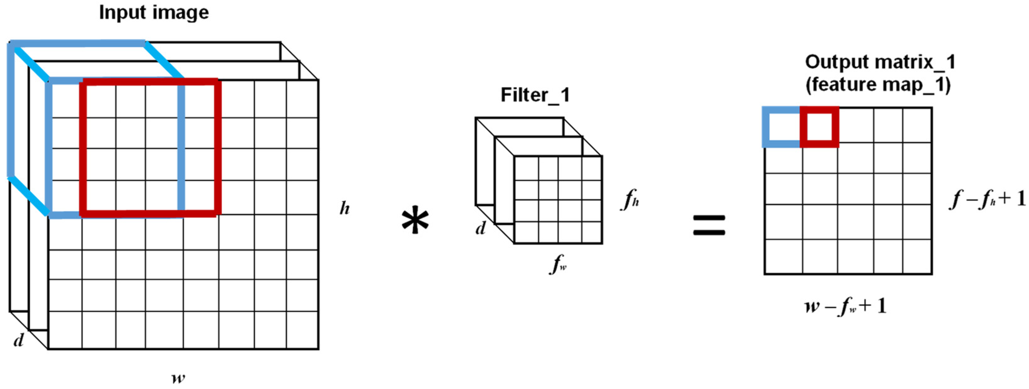
Technically, an image comes into the computer in the form of an array of pixel values with the dimension h × w × d, where h and w refer to the pixel numbers along the height direction and the width direction, and d refers to the number of color channels, which is equal to three for a common RGB color image. The convolutional layer extracts features from the raw image by reducing the input image’s size. There are many identical filters in a convolutional layer, and each filter is a relatively small matrix with the dimensions f_h × f_w × d. Generally, f_h and f_w are much smaller than h and w, while the depth of input image matrix and filter matrix should be the same. When an input image passes through a convolutional layer, it is convolved by each filter in this convolutional layer to yield a relatively small size output matrix called “feature map.” After all filters have finished the convolutions, the input image is converted into a relatively small matrix with a larger depth. The depth is equal to the number of filters in the convolutional layer, which should be determined by the user before image feeding. Figure 2 is a sketch map of the convolution operation of the image matrix with a single filter, wherein the stride (the number of pixel shifts operated by the filter over the image matrix) is equal to one. After convolution, the obtained feature map undergoes a non-linear operation by a non-linear function. Generally, the rectified linear unit (ReLU) is adopted in CNN for non-linear mapping [12] because of its faster computation and no requirement for unsupervised pre-training [13]. The ReLU function is expressed by Equation (1):

$$f(x)=\max (0,x)$$

(1)

The function of the pooling layer is to reduce the dimensions of the feature maps obtained from the convolutional layer while retaining important information. In practice, three types of pooling methods are adopted in CNN: max pooling, average pooling, and sum pooling [14]. Figure 3 illustrates the max pooling process (the stride is equal to two) that selects the maximum number from the rectified feature map. The pooling layer can further reduce image dimensions while retaining key information. Depending on the size of the input image, the combination of convolutional layer and pooling layer may be repeated several times in a CNN.

After the input image has passed though all convolutional layers and pooling layers, a flattening layer flattens the matrix generated from the last pooling layer producing a long vector. Then, this vector is fed into a regular fully connected neural network to obtain the final recognition result.

The fully connected neural network helps to translate image recognition tasks into a probability classification task, usually employing the SoftMax regression model [15] to accomplish this classification. Assuming that we prepared m images for CNN training, after passing through all convolutional layers and pooling layers, the training dataset can be denoted as $\{({\mathit{X}}^{(1)},y^{(1)}),({\mathit{X}}^{(2)},y^{(2)}),\dots ,({\mathit{X}}^{(m)},y^{(m)})\}$, wherein X⁽ⁱ⁾ represents the input features of an image, which is a vector resulting from processing by the flattening layer, and $y^{(i)}\in \{1,2,3,\dots ,k\}$ reflects the class label. In coal/gangue recognition, k = 2. The fundamental concept of a SoftMax regression is to estimate the probability of each class label for k categories, which means we have to compute the conditional probability $p(y=j|\mathit{X})$ for each $j\in (1,2,3,\dots ,k)$, given an input X. Hence, the SoftMax model is expected to output a k dimensional vector whose entries are k estimated probabilities. Generally, these k probabilities sum to one after normalization. The concrete form of this vector is as follows (denoted by h_θ(X)), wherein $1/{\displaystyle \sum _{j=1}^k{e}^{{\theta }_j^T{\mathit{X}}^{(i)}}}$ is the normalization term, and $({\theta }_1,{\theta }_2,\dots ,{\theta }_k)$ are model parameters which need to be optimized in the training process. For convenience, we stacked up $({\theta }_1,{\theta }_2,\dots ,{\theta }_k)$ as θ:

$$h_{\theta }({\mathit{X}}^{(i)})=\left[\begin{array}{l}p(y)=1|{\mathit{X}}^{(i)};\theta \\ p(y)=2|{\mathit{X}}^{(i)};\theta \\ \dots \\ p(y)=k|{\mathit{X}}^{(i)};\theta \end{array}\right]=\frac{1}{{\displaystyle \sum _{j=1}^k{e}^{{\theta }_j^T{\mathit{X}}^{(i)}}}}\left[\begin{array}{l}{e}^{{\theta }_1^T{\mathit{X}}^{(i)}}\\ e^{{\theta }_2^T{\mathit{X}}^{(i)}}\\ \dots \\ e^{{\theta }_k^T{\mathit{X}}^{(i)}}\end{array}\right]$$

(2)

Parameter optimization is the process whereby the value of the model cost function is reduced. For a SoftMax model, the cost function can be written as Equation (3), wherein m is the number of input data, which is the length of the flattened vector. In fact, this shows the “pure” cost function in this study without adding any regular term inside. For convenience, we defined an indicator function as 1{.}, so that 1{a true statement} = 1, while 1{a false statement} = 0.

$$J(\mathit{\theta })=-\frac{1}{m}[{\displaystyle \sum _{i=1}^m{\displaystyle \sum _{j=1}^{k}1\{y^{(i)}=j\}}}\log \frac{e^{{\mathit{\theta }}_j^T{\mathit{X}}^{(i)}}}{{\displaystyle \sum _{q=1}^k{e}^{{\mathit{\theta }}_q^T{\mathit{X}}^{(i)}}}}]$$

(3)

By now, there is no closed-form way to obtain the minimum value for the cost function $J(\mathit{\theta })$. Thus, the gradient descent is a common method to seek the minimum value for $J(\mathit{\theta })$. The gradient of $J(\mathit{\theta })$ is expressed by Equation (4):

$${\nabla }_{{\mathit{\theta }}_j}J(\mathit{\theta })=-\frac{1}{m}{\displaystyle \sum _{i=1}^m[{\mathit{X}}^{(i)}(1\{y^{(i)}=j\}-p(y^{(i)}=j|{\mathit{X}}^{(i)};\mathit{\theta }))]}$$

(4)

At the beginning of training, we initialized the parameter $\mathit{\theta }$. Then, for each iteration, we updated the parameter in Equation (5) until the $J(\mathit{\theta })$ converged to the minimum value; in Equation (5), $\alpha$ is the learning rate and is usually a number between 0 and 1. In practice, we were likely to obtain a local minimum rather than a global minimum for $J(\mathit{\theta })$. Hence, we had to employ some special strategies, for example, adding a regular term to the cost function. However, the strategies for avoiding local minima as well as alleviating overfitting were out of the scope of this paper.

$${\mathit{\theta }}_j:={\mathit{\theta }}_j-\alpha ·{\nabla }_{{\mathit{\theta }}_j}J(\mathit{\theta })$$

(5)

3. Model Construction for Coal/Gangue Recognition

Although we elaborated on the architecture of CNN and its training process in Section 2, it is actually impractical to construct a CNN from scratch because of the following reasons. First, it is necessary to have mass input data to ensure a valid updating of the parameters of CNN in the training process. In a CNN architecture, trainable parameters are entries in filters for each convolutional layer and weights and biases for fully connected layers. To demonstrate the massive scale of embedded parameters, we considered a toy CNN with only five convolutional layers inside. In this case, if the input image is the RGB image, the filter size in each convolutional layer is 3 × 3, and the filter number in each convolutional layer is 32. The trainable parameters in each convolutional layer are 32 × (3² × 3 + 1), 32 × (3² × 32 + 1), 32 × (3² × 32 + 1), 32 × (3² × 32 + 1), and 32 × (3² × 32 + 1), which is 37,888 in total. In practice, an industrial-strength CNN has much more parameters than this toy CNN. For example, the ImageNet [11] developed for image classification has 60 million parameters and employs 1.2 million images as input data to guarantee a valid learning of the parameters. Moreover, an industrial-strength CNN requires a super-strong computer to conduct training, which could never be accomplished by a PC. The ImageNet was trained on a strong GPU-based computer for eight weeks.

Transfer learning [16] provides an alternative strategy to address the concern of building a fresh CNN under the condition of shortage of qualified image resource and computing power. Using transfer learning, it is possible to reuse a CNN model pre-trained in a related source task as a starting point for another task, instead of building a brand-new CNN from scratch. Transfer learning is always applicable when enough training data and a strong computer are not available.

As shown in Section 2, the combination of convolutional layers and pooling layers in a CNN is used to convert a raw image to a flattened vector, which virtually plays the role of image feature extractor. The fully connected layer at the tail of CNN is a general multi-layer perceptron classifier. On the basis of this intuition, we imported a pre-trained CNN from a related task domain and removed the fully connected layers while retaining the convolutional layers and pooling layers. Then, we constructed the new fully connected layers for our own task. The new training process actually updated the parameters in this newly built fully connected layer, taking advantage of our relatively small database. Millions of weights and biases in convolutional layers and pooling layers were kept fixed in the new training process. Figure 4 is the flowchart of transfer learning in this study.

The source model we employed in this study was VGG16 [17], developed at Oxford University. This huge CNN model comprises 16 convolutional layers (weight layers) and several pooling layers, as well as three fully connected layers connecting a SoftMax classifier at the tail. The data source of VGG16 includes more than 1.3 M images which belong to 1000 categories. The model training was conducted on a powerful GPU-based computer, taking about eight weeks to update more than 160 M parameters. After training, this model achieved classification accuracy of 70.1% (top 1) and 90% (top 5) on a test dataset which included 100 K images.

The Keras [18], a deep learning library based on Python, was employed to recode the VGG16 original model (saved on a local PC in the form of Python code). All fully connected layers were replaced by our custom structure which comprised two fully connected layers with 256 neuros each and a SoftMax classifier at the tail. For each fully connected layer, we also used the ReLU function as the activation function.

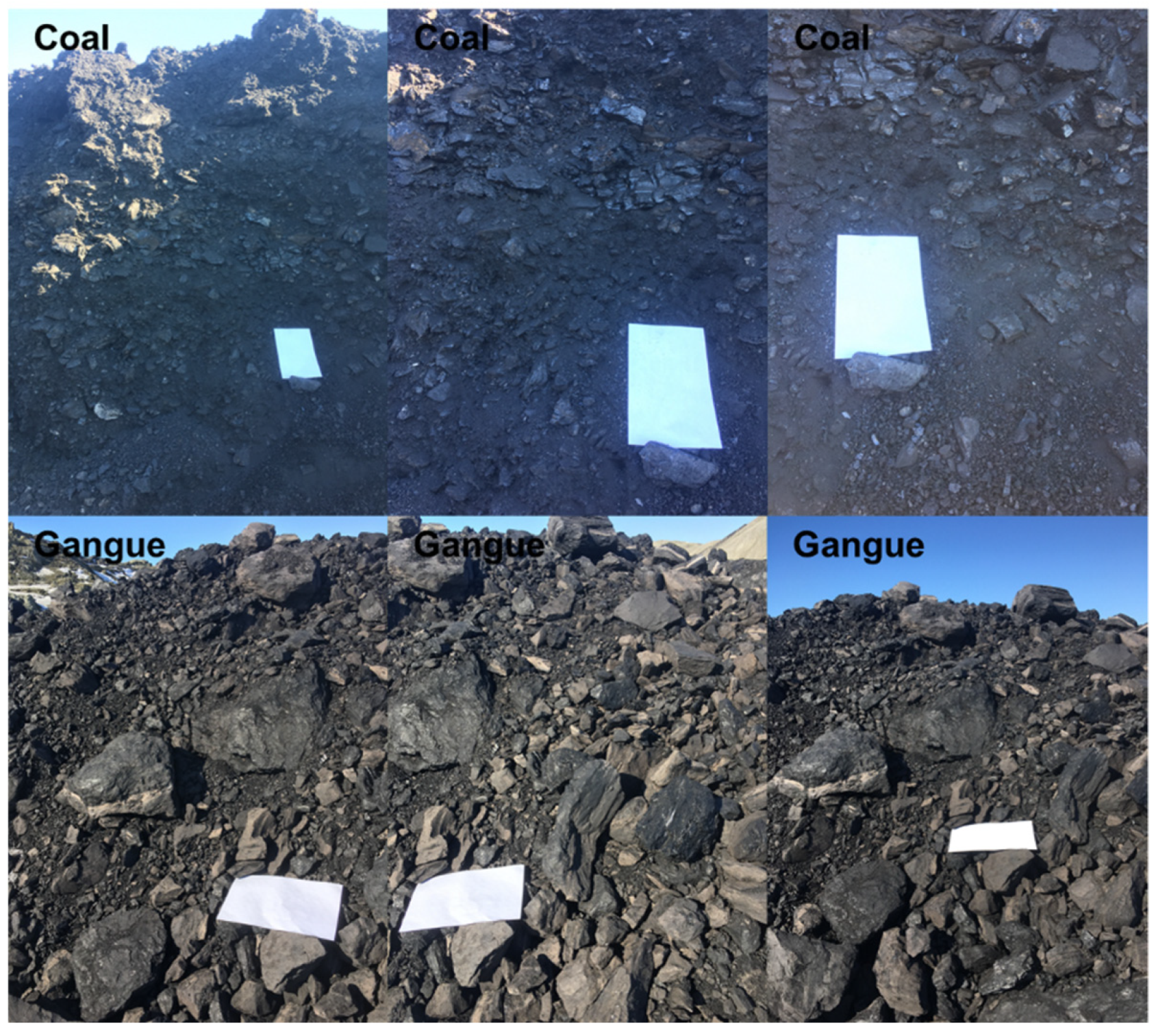
The training dataset of coal and gangue images were from several resources, mainly internet and publications. Both coal and gangue had 120 images, and each category includesd100 images for model training and 20 images for model validation. Figure 5 shows image samples for coal and gangue. Validation images were not involved in the training process and were used for measuring model performance.

Following the architecture of VGG16, all collected coal and gangue images needed to be restructured to the size of 224 × 224 × 3 (width × height × channels) to meet the VGG16 input. After the image passed through the feature extractor, the image size was 7 × 7 × 512; the image was then flattened to 1 × 25,088 before it entered into the fully connected layers. For the new CNN model, consisting of the combination of the VGG16 feature extractor and our custom fully connected layers, only the parameters in fully connected layers were updated in the training process, while the parameters in the VGG feature extractor were kept fixed. The trainable parameters included 6,488,576 weights and 514 biases.

The strategy of gradient descent was used to update the training parameters in the training process. To tradeoff the computational efficiency and image classification accuracy, mini-batch gradient descent served to implement parameter optimization. The training dataset was split into small batches, which were used to calculate training error and model parameters. In this study, the batch size was set to five, considering the scale of the training dataset. The entire training process continued for 50 epochs.

4. Model Performance and Results Discussion

In this study, it took 460 s to train our CNN on a regular PC (an Internation Core i7 processor and no discrete graphics processing units). Figure 6 illustrates the change of distributions, both weights and biases, for each fully connected layer as well as for the SoftMax layer in the training process. Before training, the weights in each layer were randomly initialized according to a normal distribution (mean = 0, std = 0.5), while biases in each layer were initialized as zero. For each subfigure, the bottom axis represented the values of weights/biases, and the left axis reflected the number of epochs. For example, in Figure 6a, when the training process had proceeded 25 epochs, there were approximately 5 × 10⁵ weights around the value of −0.01. In layer 1, the weights followed a plateaued normal distribution, where most weights were concentrated in the range [−0.02–0.02]. Layer 1 biases exhibited an obvious bimodal distribution, with the lower peak located near 0.0001, and the higher peak located near −0.0007. In layer 2, we still observed a normal distribution for weights, but with a wider plateau. The bias distribution changed from the bimodal distribution in layer 1 to the unimodal distribution, with a spike around 0.0001. For the SoftMax layer, the weights did not follow the normal distribution, but a distribution more analogous to a multimodal one. Biases in this layer exhibited two isolated mountain-like shapes in each epoch, since there were only two weights in the SoftMax layer. We can directly observe the values of two biases in Figure 6f.

For all six subfigures, after nearly 30 epochs, the weights and biases were marginally changed, which indicated that our CNN converged from the 30th epoch. On the other hand, the weights and biases did not show tremendous changes even before the 30th epoch, which implies that our CNN did not release its full potential. An obvious reason which could explain these two observed phenomena could be that our training samples were limited. Only 100 images for each category were collected for model training. The shortage of training samples resulted in a premature convergence in this study and also in a less effective parameter optimization for the CNN.

After 50 epochs of training, we plotted the model accuracy and model loss for both training samples and validation samples, as shown in Figure 7. It is worth noting that 40 validation samples were not involved in training, which meant they were never seen by our model. Not surprisingly, the training accuracy and training loss reached one and zero, respectively, as the training was completed. Validation accuracy experienced fluctuations in the first 30 epochs and stabilized after 30 epochs when, finally, the accuracy of 0.825 was achieved. Analogously, validation loss stabilized after fluctuation in the early training process. This figure also shows that the CNN converged after the 30th epoch, which confirmed the conclusion we obtained from Figure 6. Considering the size of the training dataset, 0.825 was an acceptable validation accuracy for our CNN. As indicated in the aforementioned analysis, if with more training images, the accuracy would be improved. Also, we tried tuning hyperparameters such as batch size, learning rate, and activation function to improve the model’s performance but achieved limited benefit. Therefore, in this study, increasing the training samples was the most effective and straightforward strategy to enhance our model’s performance.

We picked several misclassified images from the validation samples, as shown in Figure 8. We failed to identify by naked eye any feature that could be responsible for misclassification of these images. Humans may be able to distinguish differences between two images depending on memory and experience. By contrast, computers can quantize differences by complex computing, which is impossible for humans. This property guarantees the robustness of computers in different image recognition tasks. Nevertheless, even though we achieved satisfying outcomes from the CNN model, we could not figure out where the correct and the wrong outcomes came from. This so-called “black-box” property [19] has become a must-solve problem for deep learning.

Since only a small portion of our validation pictures were from the field, which is a limit for demonstrating the model applicability in engineering practice, we took photos (Figure 9) from a washing plant stockpile at a coal mine to test the model performance. These photos included three coal photos and three gangue photos which were shot after coal separation. Our model accurately recognized these six photos without any misclassification. Although there was a relatively small number of test samples, this demonstrated that the model can be used in engineering practice.

We addressed the problem of distinguishing coal and gangue using transfer learning and a CNN model in this study. However, it seemed that we only fulfilled a “hindsight” task, meaning that we could correctly distinguish coal and gangue only after they were separated. Another issue is how to use this model in the coal/gangue washing process to realize a real automatic classification. This may require the development of both hardware and software, which is out of this paper’s scope. Regardless, the correct recognition of coal and gangue by our model lays a solid foundation for follow-up studies on this topic.

5. Conclusions

This study built a deep learning model using a convolutional neural network and transfer learning to distinguish coal and gangue images. A recognition accuracy of 82.5% was realized for validation pictures after the model was trained on a relatively small database (each category included 100 training images and 20 validation images). This study also delivered satisfactory recognition results using this model for engineering field pictures.

Different from current mainstream coal/gangue image reorganization technologies, CNN can extract image features by analyzing every image pixel, which avoids subjective and incomplete feature extraction. In this study, each input image was denoted by a 1 × 25,088 vector through a series of convolution and pooling implementations which, to a large extent, retained the image’s characteristics. Image reorganization using a CNN has no special requirement for image features such as the size of the object in the image, photography location, and light intensity. As shown in this paper, our training data were from many sources, including internet and published papers. This property of the CNN can guarantee the easy collection of training images, which virtually enhances the generalization of the CNN. No explicit discriminate standard for image recognition exists in the CNN model, which could improve the model’s flexibility in dealing with some ambiguous materials like the materials of this study.

This paper also identified the mass trainable parameters in the CNN and, further, imported a transfer learning strategy for a valid CNN model training under the condition of a small training database. A strong image identification model, VGG16, was used as a source model for transfer learning in this study. All fully connected layers in VGG16 were replaced by our custom layers, while convolutional layers and pooling layers were retained as the feature extractor. Since we fixed all parameters of retained convolutional layers and pooling layers, all trainable parameters in our restructured model decreased to 6,488,576 weights and 514 biases, which made it possible to train our model possible using a small database.

The model training continued for about 460 s with 50 epochs. From the observation of some figures reflecting the training process, we found that after about 30 epochs, the model virtually converged and, thus, did not release its full potential. Although this model achieved a recognition accuracy of 82.5% for validation pictures, we can assert that the accuracy should boost if a larger database is employed.

References

- Bugge, J.; Kjær, S.; Blum, R. High-efficiency coal-fired power plants development and perspectives. Energy 2006, 31, 1437–1445. [Google Scholar] [CrossRef]
- Hobson, D.M.; Carter, R.M.; Yan, Y.; Lv, Z. Differentiation between coal and stone through image analysis of texture features. In Proceedings of the 2007 IEEE International Workshop on Imaging Systems and Techniques, Krakow, Poland, 5 May 2007. [Google Scholar]
- Luo, Z.; Fan, M.; Zhao, Y.; Tao, X.; Chen, Q.; Chen, Z. Density-dependent separation of dry fine coal in a vibrated fluidized bed. Powder Technol. 2008, 187, 119–123. [Google Scholar] [CrossRef]
- Woodburn, E.T. (Ed.) Frothing in Flotation II: Recent Advances in Coal Processing (Vol. 2); CRC Press: Routledge, UK, 2018. [Google Scholar]
- Gao, K.; Du, C.; Wang, H.; Zhang, S. An efficient of coal and gangue recognition algorithm. Int. J. Signal Process. Image Process. Pattern Recognit. 2013, 6, 345–354. [Google Scholar]
- Yu, L.; Zheng, L.; Du, Y.; Huang, X. Image Recognition Method of Coal and Coal Gangue Based on Partial Grayscale Compression Extended Coexistence Matrix. J. Huaqiao Univ. 2018, 39, 906–912. (In Chinese) [Google Scholar] [CrossRef]
- Li, W.; Wang, Y.; Fu, B.; Lin, Y. Coal and coal gangue separation based on computer vision. In Proceedings of the 2010 Fifth International Conference on Frontier of Computer Science and Technology (FCST), Changchun, China, 18–22 August 2010; pp. 467–472. [Google Scholar]
- Bianco, S.; Buzzelli, M.; Mazzini, D.; Schettini, R. Deep learning for logo recognition. Neurocomputing 2017, 245, 23–30. [Google Scholar] [CrossRef] [Green Version]
- Schmidhuber, J. Deep learning in neural networks: An overview. Neural Netw. 2015, 61, 85–117. [Google Scholar] [CrossRef] [PubMed] [Green Version]
- Cireşan, D.; Meier, U.; Schmidhuber, J. Multi-column deep neural networks for image classification. arXiv 2012, arXiv:1202.2745. [Google Scholar]
- Krizhevsky, A.; Sutskever, I.; Hinton, G.E. Imagenet classification with deep convolutional neural networks. In Proceedings of the 25th International Conference on Neural Information Processing Systems, Lake Tahoe, NV, USA, 3–6 December 2012; pp. 1097–1105. [Google Scholar]
- Bradski, G.; Kaehler, A. Learning OpenCV: Computer Vision with the OpenCV Library; O’Reilly Media, Inc.: Champaign, IL, USA, 2008. [Google Scholar]
- Glorot, X.; Bordes, A.; Bengio, Y. Deep sparse rectifier neural networks. In Proceedings of the Fourteenth International Conference on Artificial Intelligence and Statistics, Ft. Lauderdale, FL, USA, 11–13 April 2011; pp. 315–323. [Google Scholar]
- Szeliski, R. Computer Vision: Algorithms and Applications; Springer Science & Business Media: Berlin, Germany, 2010. [Google Scholar]
- Witten, I.H.; Frank, E.; Hall, M.A.; Pal, C.J. Data Mining: Practical Machine Learning Tools and Techniques; Morgan Kaufmann: Burlington, MA, USA, 2016. [Google Scholar]
- Thrun, S.; Pratt, L. Learning to Learn; Springer Science & Business Media: Berlin, Germany, 2012. [Google Scholar]
- Simonyan, K.; Zisserman, A. Very deep convolutional networks for large-scale image recognition. arXiv 2014, arXiv:1409.1556. [Google Scholar]
- van Merriënboer, B.; Bahdanau, D.; Dumoulin, V.; Serdyuk, D.; Warde-Farley, D.; Chorowski, J.; Bengio, Y. Blocks and fuel: Frameworks for deep learning. arXiv 2015, arXiv:1506.00619. [Google Scholar]
- LeCun, Y.; Bengio, Y.; Hinton, G. Deep learning. Nature 2015, 521, 436–444. [Google Scholar] [CrossRef] [PubMed]
Figure 1.
The flowchart of a convolutional neural network (CNN) for image recognition.
Figure 2.
Convolution operation by a single filter.
Figure 3.
A pooling operation with the stride equaling two.
Figure 4.
Flowchart of transfer learning.
Figure 5.
Coal and gangue images from the database.
Figure 6.
Updating process of trainable parameters in CNN training.
Figure 7.
Model accuracy and loss for both training and validation.
Figure 8.
A portion of misclassified images from the validation database.
Figure 9.
Photos of coal and gangue from a washing plant stockpile.
© 2019 by the authors. Licensee MDPI, Basel, Switzerland. This article is an open access article distributed under the terms and conditions of the Creative Commons Attribution (CC BY) license (http://creativecommons.org/licenses/by/4.0/).
Share and Cite
MDPI and ACS Style
Pu, Y.; Apel, D.B.; Szmigiel, A.; Chen, J. Image Recognition of Coal and Coal Gangue Using a Convolutional Neural Network and Transfer Learning. Energies 2019, 12, 1735. https://doi.org/10.3390/en12091735
AMA Style
Pu Y, Apel DB, Szmigiel A, Chen J. Image Recognition of Coal and Coal Gangue Using a Convolutional Neural Network and Transfer Learning. Energies. 2019; 12(9):1735. https://doi.org/10.3390/en12091735
Chicago/Turabian StylePu, Yuanyuan, Derek B. Apel, Alicja Szmigiel, and Jie Chen. 2019. "Image Recognition of Coal and Coal Gangue Using a Convolutional Neural Network and Transfer Learning" Energies 12, no. 9: 1735. https://doi.org/10.3390/en12091735
Note that from the first issue of 2016, this journal uses article numbers instead of page numbers. See further details here.