Short-Term Electricity Load Forecasting Model Based on EMD-GRU with Feature Selection

Abstract

Many factors affect short-term electric load, and the superposition of these factors leads to it being non-linear and non-stationary. Separating different load components from the original load series can help to improve the accuracy of prediction, but the direct modeling and predicting of the decomposed time series components will give rise to multiple random errors and increase the workload of prediction. This paper proposes a short-term electricity load forecasting model based on an empirical mode decomposition-gated recurrent unit (EMD-GRU) with feature selection (FS-EMD-GRU). First, the original load series is decomposed into several sub-series by EMD. Then, we analyze the correlation between the sub-series and the original load series through the Pearson correlation coefficient method. Some sub-series with high correlation with the original load series are selected as features and input into the GRU network together with the original load series to establish the prediction model. Three public data sets provided by the U.S. public utility and the load data from a region in northwestern China were used to evaluate the effectiveness of the proposed method. The experiment results showed that the average prediction accuracy of the proposed method on four data sets was 96.9%, 95.31%, 95.72%, and 97.17% respectively. Compared to a single GRU, support vector regression (SVR), random forest (RF) models and EMD-GRU, EMD-SVR, EMD-RF models, the prediction accuracy of the proposed method in this paper was higher.

1. Introduction

The electric-power industry, a basic industry supporting state construction, plays an increasingly important role in our daily life. Stable and uninterrupted high-quality electric energy provides a guarantee for the stable operation of industry and society [1]. Therefore, in order to ensure the stable operation of the power system and provide economic and reliable power for the market, it is necessary to accurately predict the change of load when planning the power system. Furthermore, the prediction also guides a reasonable production schedule.

Electricity load forecasting is a process of predicting future load changes by analyzing historical load data. It explores the dynamic changes of load data by qualitative and quantitative methods, such as statistics, computer science, and empirical analysis [2]. Based on the time horizon of prediction, the load forecasting can be classified into four categories: long-term forecasting, medium-term forecasting, short-term forecasting, and ultra-short-term forecasting [3]. Short-term electricity load forecasting is one of the main tasks for the grid dispatching operation department, and its accuracy is closely related to the formulation of dispatching plans and the proposal of transmission schemes. However, many factors affect the change of short-term load, which causes the load series to be highly non-linear and non-stationary, thus high-precision prediction of short-term load is a challenging task [4].

Since the middle of the 20th century, many researchers have devoted work to the research of short-term load forecasting, and they have proposed many effective models and solutions [5]. In previous studies, short-term load forecasting methods mainly have included traditional statistical methods, artificial intelligence methods based on machine learning, and combination forecasting methods [6]. Traditional methods include multivariate linear regression, time series, exponential smoothing, etc. Machine learning methods include artificial neural networks (ANN), support vector machines (SVM), random forest (RF), etc. [3]. Combination forecasting methods include model combination based on prediction mechanism and weighted combination based on forecasting results [7].On account of the high non-linear and the non-stationary features, many models and methods have certain limitations for short-term load forecasting. For example, traditional methods have a weak ability to process non-linear data, while machine learning methods need to filtrate timing features manually. Combination forecasting methods can form more adaptable methods by combining the advantages of various methods. Among them, the signal decomposition methods that decompose the original load series into different load components can effectively improve the prediction accuracy. However, directly modeling and forecasting the decomposed time series components separately will give rise to multiple random errors and generate a large amount of forecasting workload.

In this paper, an empirical mode decomposition-gated recurrent unit (EMD-GRU) forecasting model with feature selection is proposed to improve the prediction accuracy of short-term electricity load. Its main contributions are as follows:

• Correlation analysis was performed on the sub-series obtained by EMD using the Pearson correlation coefficient method. Since the decomposed sub-series contained different features of the original load series, they had different effects on the fluctuation of the original load series. The components with high correlation with the original load series were selected by Pearson correlation coefficient method as the input features of the prediction model.
• An EMD-GRU load forecasting model with feature selection was proposed. The selected sub-series were input into the GRU network together with the original load series to establish the final prediction model, which avoided the multiple random errors introduced by modeling the multiple sub-series separately, and reduced the overall model complexity. At the same time, the GRU network with unique network structure in the recurrent neural network (RNN) was used as the prediction model, which solved the problem of gradient disappearance of the RNN in dealing with long-span time series, had better processing effect on time series, and achieved higher prediction accuracy.
• Compared with the three single models, including GRU, SVR and RF, and the three hybrid models including EMD-GRU, EMD-SVR, and EMD-RF, the proposed method had the best prediction performance.

The remaining of this paper is organized as follows: Section 2 describes some relevant works in the field of short-term load forecasting. Section 3 introduces the theoretical background on forecasting methods and presents the EMD-GRU method with feature selection proposed in this paper. Section 4 introduces the experimental results and analysis of four data sets from different regions. Finally, in Section 5, the conclusion is stated.

2. Related Work

As the electric load series is non-linear, unstable and relatively random, many models and methods have certain limitations in short-term load forecasting [8].

Since the mid-20th century, various statistical-based linear time series prediction methods have been proposed, and these methods generally need a precise mathematical model to present the relationship between load and input factors. Haida [9] proposed a regression-based daily peak load forecasting method and conversion technique. Khashei [10] predicted the hourly load changes by establishing an autoregressive integrated moving average model (ARIMA). Holt [11] used an exponentially weighted moving average prediction model to predict non-seasonal and seasonal series with additive or multiplicative error structures. However, the forecasting model based on statistical method is relatively simple and requires high stability of load series, which cannot accurately reflect the non-linear characteristics of load data.

With the development of artificial intelligence technology, machine learning methods, such as ANN, SVM, and RF, have been widely used in the field of short-term load forecasting [3]. Reference [12] proposed a short-term load forecasting method based on improved variable learning rate back propagation (BP) neural network, and the experiment results show the method has high accuracy and real-time performance. Fu Y [13] used the SVM to predict the hourly electricity load of a building and achieved good results. In Reference [14], RF was used to predict the load for the next 24 h, and the predicted performance of the model was analyzed in detail. Although the machine learning method performs better in nonlinear relationship of the load series and has achieved good results in the field of load forecasting, there are still some defects. Load series is a complex time series, and the machine learning method has poor processing ability for timing features and requires manual filtrating the timing features [15].

The flourishing development of deep learning provides researchers with new ways to solve this problem. Deep learning method mainly refers to the deep neural network which contains multiple hidden layers and has specific structure and training method. It has been widely used in many fields, such as speech recognition [16] and image processing [17]. At present, it has also been discussed in the field of electricity load forecasting. Mocanu [18] used the deep belief network composed of conditional restriction Boltzmann machine (CRBM) to predict the load of a single residential building. Compared with the shallow artificial neural network and support vector machine, the results improved a lot. Reference [19] established a predictive model based on long short-term memory neural network (LSTM) to predict the short-term electricity consumption of individual residential users. Aowabin Rahman [20] used RNN to predict hourly consumption of a safety building in Utah and residential buildings in Texas, and the results have lower relative errors compared to multilayer perceptron networks. Due to the limited learning ability of deep belief network for time series features, Recurrent Neural Network has been heated discussed in short-term load forecasting for its unique structure. However, RNN has been proven to have the problems of gradient explosion and disappearance. Based on the RNN, the GRU network solves the problem of gradient explosion and disappearance of RNN by adding the gate structure to control the influence of the previous time [21], so that it can better process the time series.

In recent years, various combination models have been introduced to improve the accuracy of short-term electricity load forecasting. Among them, the combination of signal decomposition method and machine learning method has been widely studied [22]. Rana [23] used wavelet neural network to decompose the load series into sub-series with different frequencies, and then established a prediction model for each sub-series, and obtained more accurate prediction results. However, it is necessary to choose the wavelet basis function manually for the wavelet transform. EMD is another method of signal decomposition. Instead of setting basis function in advance, it can decompose the signal according to the characteristics of the data itself, and the basis function is directly generated from the signal itself in the process of decomposition [24]. Each sub-series contains only part characteristic of the original load series, which makes it much simpler than the original load series, so that more accurate prediction results can be obtained, and the EMD method has been widely used in the field of load forecasting. Guo [25] used the SVR and auto regression (AR) models to predict the high frequency and residual components decomposed by EMD, respectively. Jatin [26] combined the EMD method with LSTM model to forecast the load demand for a given season and date, and obtained better results than the single prediction model. The hybrid models mentioned above are mainly different in the decomposition algorithm or the prediction model, but the establish process is almost the same. Unlike most previous studies that built prediction models for each component, in this paper, the feature selection method was used to select components that were highly correlated with the original series from the decomposed sub-series as features to input the GRU prediction model.

3. Theoretical Background on Forecasting Models

3.1. Empirical Mode Decomposition

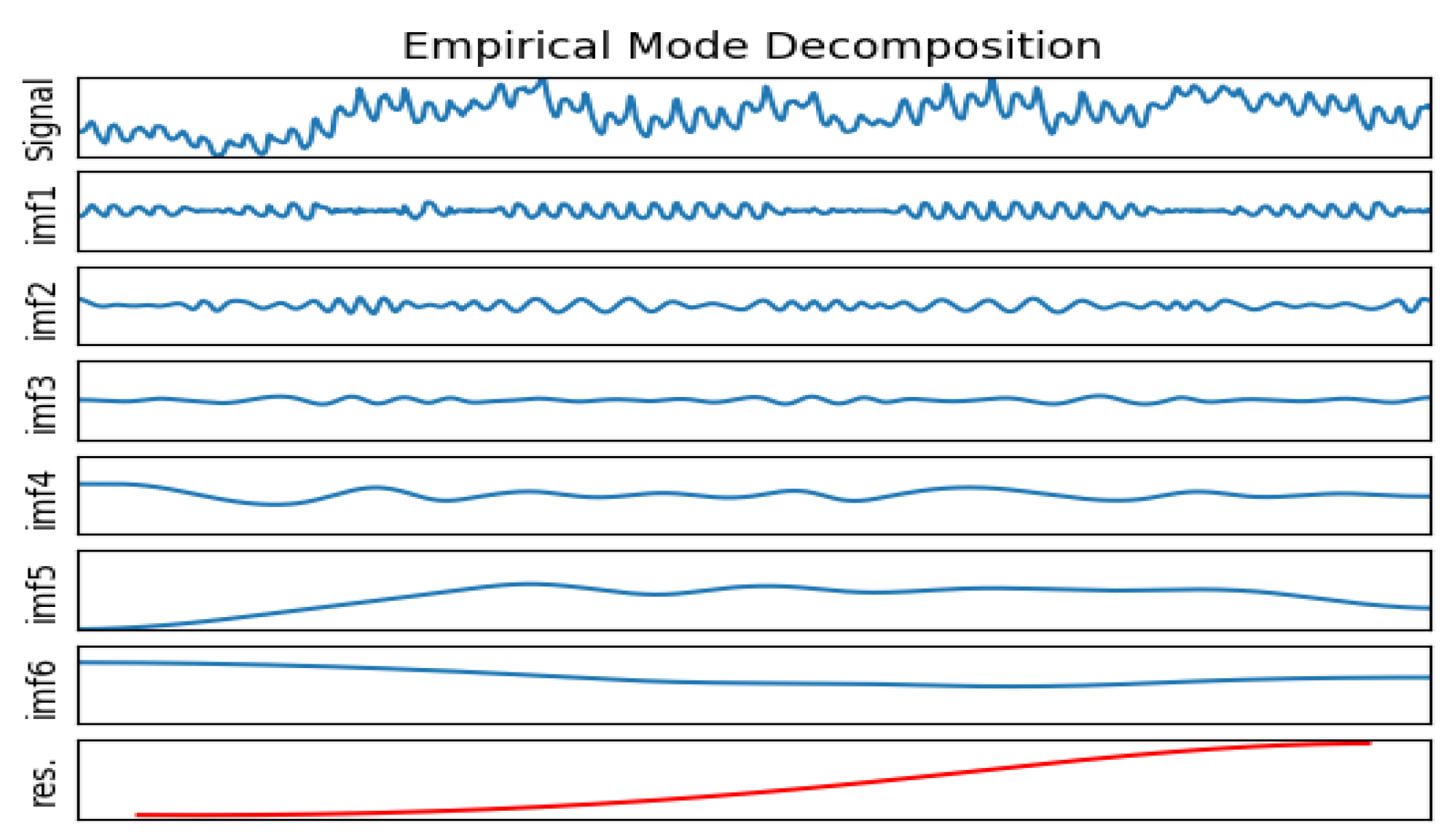
EMD is a signal processing method inventively proposed by Huang et al. [24]. This method decomposes signals according to the time scale characteristics of the data itself without presetting any basis function, which is quite different from Fourier decomposition and wavelet decomposition based on prior harmonic basis function and wavelet basis function. Thus, EMD can be applied to decomposition of any kind of signal in theory, and it has great advantages in dealing with non-stationary and non-linear data [27].

The decomposed sub-series contain a set of intrinsic mode functions (IMF) along with a residue which stands for the trend. The IMF satisfies two basic conditions: (a) The function must have the same number of local extremum points and zero-crossing points, or the maximum difference must be one; (b) at any time, the mean of the envelope of the local maximum (upper envelope) and the envelope of the local minimum (lower envelope) must be zero [28]. The procedures of EMD algorithm are shown as follows:

Step 1: Find all the maximum and minimum points of signal $X(t)$. Cubic spline interpolation is used to obtain the upper and lower envelope curves $e_{max}(t)$ and $e_{min}(t)$, and then calculate the mean of the upper and lower envelope $m(t)$, i.e., $m(t)=(e_{max}(t)+e_{min}(t))/2$;

Step 2: Calculate the difference $h(t)$ between $X(t)$ and $m(t)$, i.e., $h(t)=X(t)-m(t)$;

Step 3: Determine whether $h(t)$ satisfies the two conditions of the IMF. If it is satisfied, $h(t)$ is the first IMF, which is recorded as $im{f}_1(t)$; if not, $h(t)$ is taken as the original signal and returns to Step 1;

Step 4: Separate $im{f}_1(t)$ from the original signal: $r(t)=X(t)-im{f}_1(t)$, and if $r(t)$ is a monotone function, then $r(t)$ is regarded as residual and the iteration is stopped. Instead, $r(t)$ is returned to Step 1 as the original signal.

Finally, the original signal $X(t)$ can be expressed as the sum of several IMFs and a residual:

$$X(t)={\displaystyle \sum _{i=1}^n}im{f}_i(t)+r(t)$$

(1)

where n is the number of IMFs.

Each of the components decomposed by EMD contains only a portion of the features of the original series, which makes it much simpler than the original series. Figure 1 shows an example of a one-month load decomposition of a utility in a U.S. region. It can be seen that each component has different features.

3.2. Recurrent Neural Network and Gated Recurrent Unit Network

The Gated Recurrent Unit network is a kind of the Recurrent Neural Network [29]. Compared with the traditional neural networks, RNN has better performance for time series as it can retain the influence of previous inputs to the model and allow it participate in the calculation of the next output. However, the range of context information that can be memorized in the RNN model is actually limited. The parameter information stored in the hidden layer grows geometrically as the number of connections in the network increases, which will cause the gradient disappearance [30]. The gradient disappearance makes it difficult to train data for long spans, thus losing the ability to learn longer information in the past.

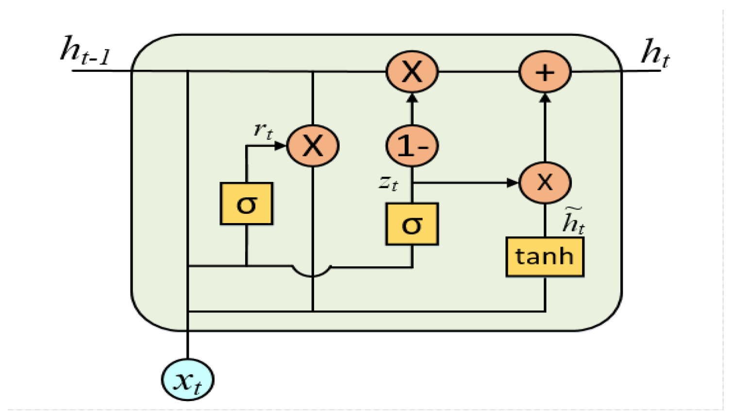
In recent years, with the deepening of the research on RNN, a variety of RNN variant structures have been proposed, where the LSTM model based on the gate structure has a great improvement on traditional RNN [31]. It solves the problem of gradient disappearance of RNN and has been widely used in the field of forecasting time series. Later, many well-known variant structures were derived on the basis of LSTM with gate structure. The GRU is one of the most popular variants of LSTM, with fewer training parameters than LSTM, while maintaining the predictive effect of LSTM. The GRU is similar in structure to the LSTM, and the difference is that the GRU reduces the internal hidden state and the associated gate structure compared to the LSTM [21]. The former has three gates, while there are only two gate structures in the GRU, that is, the update gate and the reset gate. The update gate controls the extent to which the state information of the previous moment is retained in the current state, while the reset gate determines whether the current state is to be combined with the previous information [32]. Figure 2 shows the basic structure of a GRU [33].

The formulas of GRU are represented in Equations (2)–(5):

$$z_t=\sigma ({\mathbf{W}}^{(z)}{x}_t+{\mathbf{U}}^{(z)}{h}_{t-1}),$$

(2)

$$r_t=\sigma ({\mathbf{W}}^{(r)}{x}_t+{\mathbf{U}}^{(r)}{h}_{t-1}),$$

(3)

$${\tilde{h}}_t=tanh(r_t\ast \mathbf{U}{h}_{t-1}+\mathbf{W}{x}_t),$$

(4)

$$h_t=(1-z_t)\ast {\tilde{h}}_t+z_t\ast h_{t-1},$$

(5)

where $x_t$ is the input of the hidden layer at time t , $h_t$ is the output of the current layer at time t and $h_{t-1}$ is the output at time $t-1$, $z_t$ and $r_t$ are update gate and reset gate, ${\tilde{h}}_t$ represents the set of input $x_t$ and the output $h_{t-1}$ at the previous moment. $\sigma$ and $tanh$ represent activation functions, which are Sigmoid function and hyperbolic tangent function, respectively. ${\mathbf{U}}^{(z)}$ and ${\mathbf{W}}^{(z)}$ are training parameter matrices in the update gate, ${\mathbf{U}}^{(r)}$ and ${\mathbf{W}}^{(r)}$ are training parameter matrices in the reset gate, and $\mathbf{U}$ and $\mathbf{W}$ are training parameter matrices in the process of obtaining ${\tilde{h}}_t$. “∗” represents matrix multiplication.

3.3. Proposed EMD-GRU Model with Feature Selection

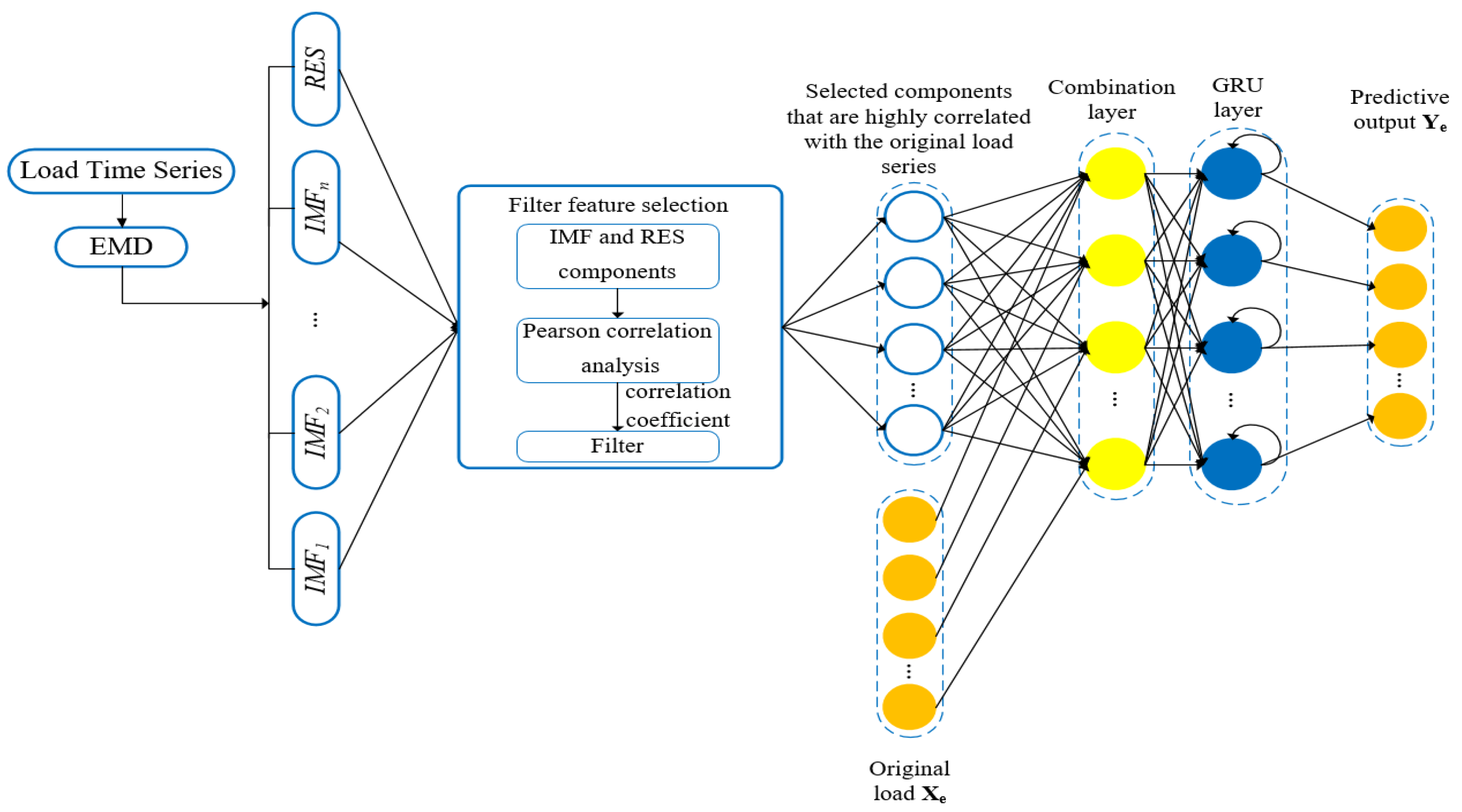
The EMD algorithm can decompose signal of different frequencies step-by-step according to the characteristics of the data itself and several orthogonal signals with periodicity and trend will be obtained. The general used prediction method based on EMD is to respectively establish prediction models for the decomposed sub-series, and then superimpose the output of each prediction model to get the final prediction result [22,25,26]. Although the prediction accuracy is improved, multiple random errors will be introduced to build prediction models for each sub-series separately, and some high frequency noise components exist in the decomposed sub-series, which will give rise to a large prediction error when modeling these sub-series, and affect the overall prediction accuracy. At the same time, the overall complexity of the model will be increased due to the establishment of multiple prediction models. In this paper, an EMD-GRU model with feature selection was proposed for short-term load forecasting. Correlation analysis was performed on the decomposed sub-series and the components with large correlation with the original series are selected as the input features of the model. On the one hand, the proposed method can avoid the occurrence of multiple random errors and improve the prediction accuracy; on the other hand, since there is only one prediction model, the number of prediction models is greatly reduced compared with the prediction models established for each sub-series, which reduces the overall complexity of the model. The procedure of the proposed method is shown as follows:

Step 1: The original load series was decomposed into several IMFs and one residual RES by EMD;

Step 2: All the IMFs and residual were used as initial feature sets, which constitute potential input variables for the predictive model;

Step 3: The Pearson correlation coefficient method was used to analyze the correlation of the initial features, and the time series components with large correlation with the original load series were selected as the input features of the prediction model;

Step 4: The features selected in the previous step were combined with the original load series to form a combined dataset. Then, the combined dataset is divided into the training set and testing set, and the specific division is given in Section 4.5. The training set is input into GRU model to train the prediction model, and then the testing set is input into the prediction model to evaluate the prediction results.

Figure 3 shows the overall structure of the model.

The time series components obtained by EMD constitute the initial feature set, and then the initial feature set is filtered by the feature selection method. As a filter feature selection method, Pearson correlation coefficient has strong generality and low complexity, and it has strong advantages in dealing with large-scale data sets and can eliminate a large number of irrelevant features in a short time. Therefore, it is often used for feature selection of the whole data set [34]. The formulation of Pearson correlation coefficient is represented in Equation (6):

$$\gamma =\frac{{\displaystyle \sum _{i=1}^n}(x_i-\stackrel{-}{x})(y_i-\stackrel{-}{y})}{\sqrt{{\displaystyle \sum _{i=1}^n}{(x_i-\stackrel{-}{x})}^2{\displaystyle \sum _{i=1}^n}{(y_i-\stackrel{-}{y})}^2}},$$

(6)

where $\gamma$ is the correlation coefficient and represents the correlation between data. $x_i$ and $y_i$ represent the sample points, $\overline{x}$ and $\overline{y}$ represent the sample mean, and n is the number of samples. The Pearson correlation coefficient method uses correlation indicators to score individual features and filtrates the features with scores greater than the threshold. Specifically, the correlation between each component then the original load series is calculated, and the component with correlation less than the threshold is removed, and the component with correlation larger than the threshold is selected as the input feature of the prediction model. The input of the model is as follows:

$$\mathbf{X}=\{im{f}_1,im{f}_2,\dots ,im{f}_{n-1},res\},$$

(7)

$$\mathbf{Data}\_\mathbf{input}=\{{\mathbf{X}}_{\mathbf{e}},{\mathbf{X}}_{\mathbf{f}}\},$$

(8)

where $\mathbf{X}$ represents the initial feature set, $im{f}_i$ and $res$ represent the decomposed IMF components and residual, respectively, n represents the total number of decomposed time series components, ${\mathbf{X}}_{\mathbf{e}}$ represents the historical load data, and ${\mathbf{X}}_{\mathbf{f}}$ represents the feature set composed of the components selected through feature selection. $\mathbf{Data}\_\mathbf{input}$ represents the combined dataset that combines the historical load and feature set and is fed into the GRU network for training and prediction. The detailed process of proposed method is briefly explained in Algorithm 1.

Algorithm 1 FS-EMD-GRU Algorithm

1: Definitions: M: is the predicted output data length; ${\gamma }_i$: is the correlation coefficient between the ith component and the original series; $\rho$: is the threshold of correlation coefficient; 2: ${\mathbf{X}}_{\mathbf{e}}$ is decomposed by EMD algorithm and the initial feature set is obtained;            $\mathbf{X}=\{im{f}_1,im{f}_2,\dots ,im{f}_{n-1},res\}$ 3: Calculating the correlation coefficient $\gamma$ of each component and the original load series by using the Pearson correlation coefficient method; 4: Feature selection for the initial feature set: 5: if${\gamma }_i>\rho$then 6:            Put $im{f}_i$ as a feature subset in ${\mathbf{X}}_{\mathbf{f}}$; 7: else 8:            Remove the $im{f}_i$; 9: end if 10: Get the input feature set ${\mathbf{X}}_{\mathbf{f}}$; 11: Combine the original series and the feature subset as the input set of the prediction model:                 $\mathbf{Data}\_\mathbf{input}=\{{\mathbf{X}}_{\mathbf{e}},{\mathbf{X}}_{\mathbf{f}}\}$ 12: Divide $\mathbf{Data}\_\mathbf{input}$ into training set and testing set, and send it into GRU model training and testing in batches; 13: Get the final predicted output ${\mathbf{Y}}_{\mathbf{e}}$:                 ${\mathbf{Y}}_{\mathbf{e}}={[e_1,e_2,\dots ,e_M]}^T$ 14: END

4. Result and Discussion

In this paper, the effectiveness of the proposed method is compared with the other six methods: GRU, SVR, RF, EMD-GRU, EMD-SVR, and EMD-RF.

4.1. Load Datasets

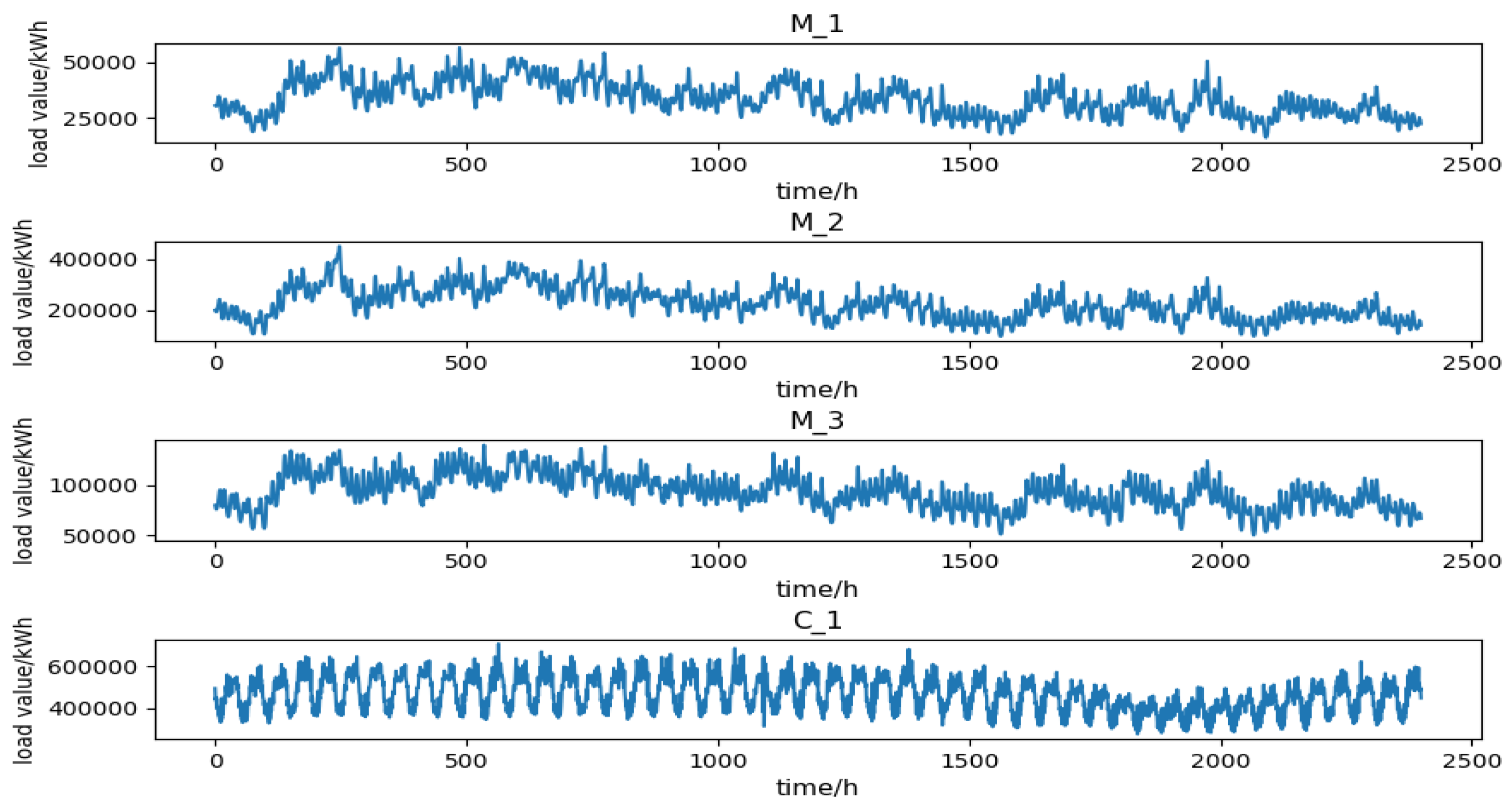
The proposed model was evaluated using daily load data from U.S. Public Utilities [35] and a region in northwestern China. The U.S. Public Utilities Data Set uses three-year daily load data from three different regions and is recorded every hour. Our model used data recorded from January 2004 to December 2006. And the data set of a region in Northwest China is based on 19-month daily load data, which is recorded every half hour, from January 2016 to July 2017. Figure 4 shows the partial load time series corresponding to four regions, and it can be seen that the load series presents obvious non-stationary and certain periodicity. The descriptive statistics of the four datasets are shown in

Table 1. Descriptive statistics of four electricity load datasets.

	M_1	M_2	M_3	C_1
Data Set Name	U.S. Public Utilities Sector 1	U.S. Public Utilities Sector 2	U.S. Public Utilities Sector 3	Region in Northwest China
Total sample size	26,304	26,304	26,304	27,744
Mean (kWh)	32,175.36	208,383.49	86,607.58	506,546.19
Maximum (kWh)	62,178	451,096	156,366	761,989.67
Minimum (kWh)	16,177	90,621	46,291	207,713.70
Standard deviation (kWh)	7634.97	61,826.11	17,730.05	92,289.41

, including total sample size, mean, maximum and minimum, and standard deviation.

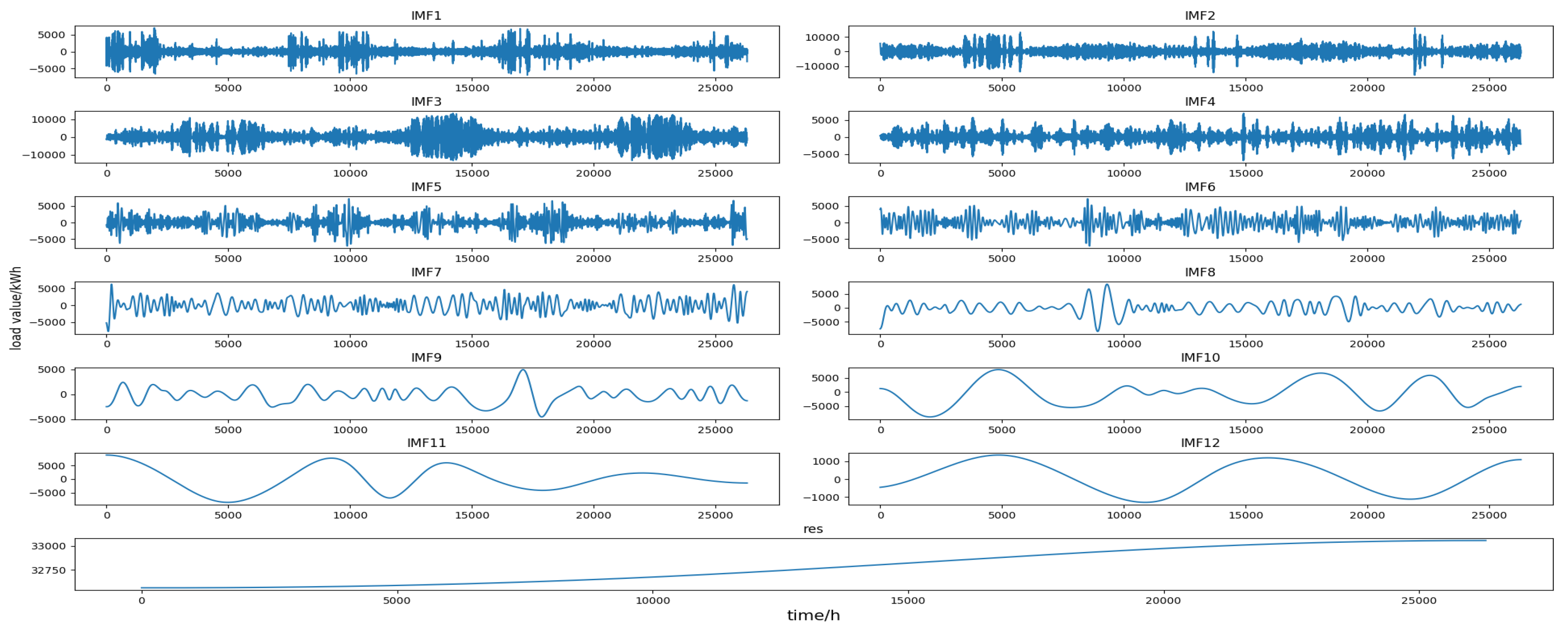
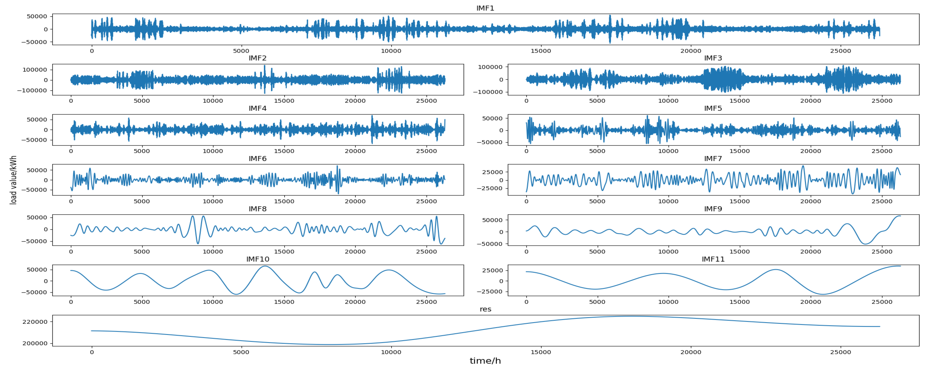
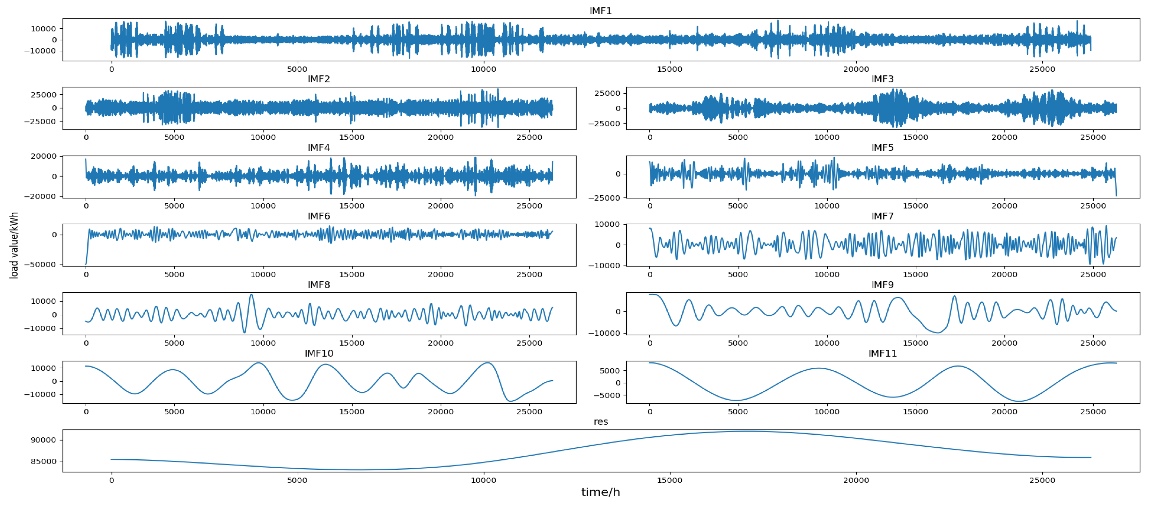
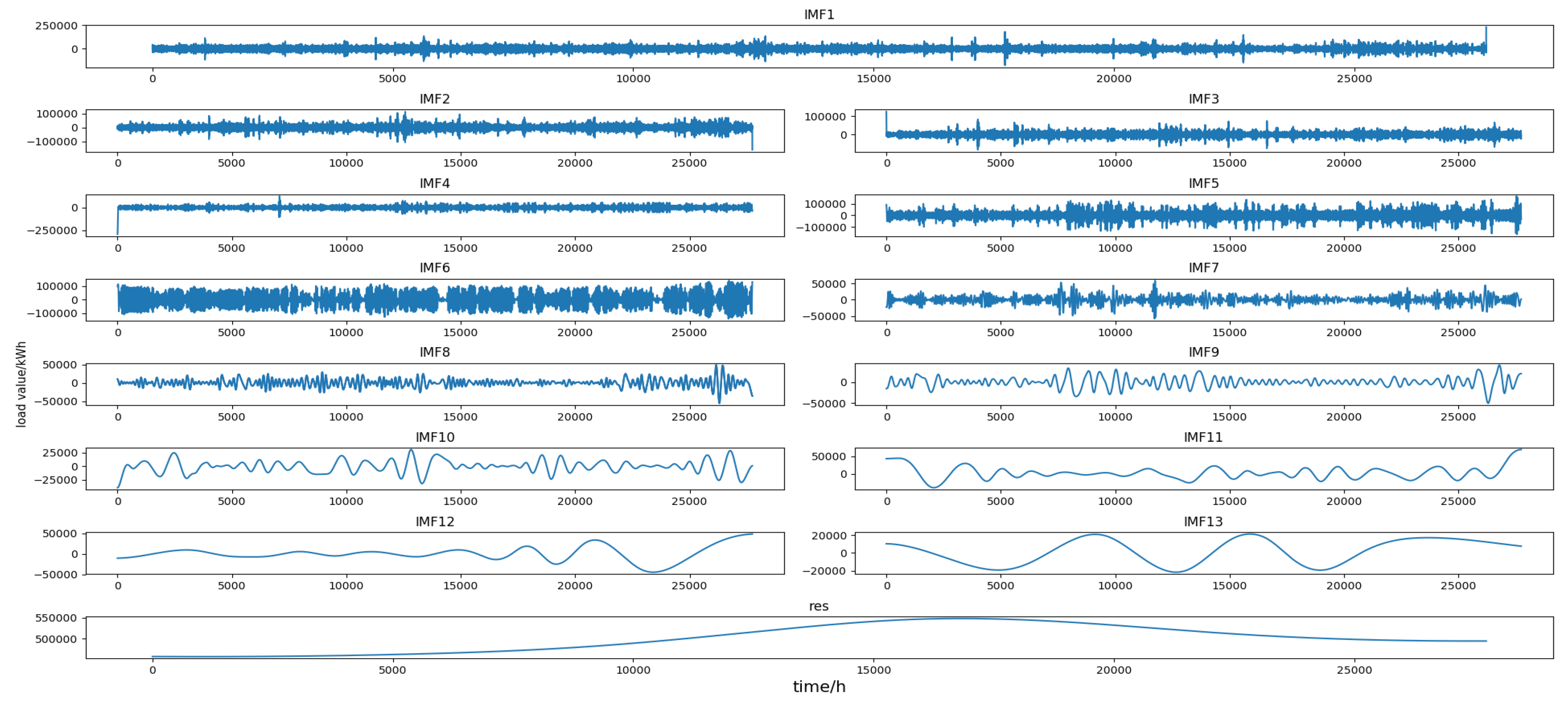
4.2. EMD Decomposition Results of Load Series

The original load series was decomposed into multiple IMF components and a residual by EMD. Each component had different trends and features that represent different features of the fluctuation of the original load series. The decomposition results of the four data sets are shown in Figure 5, Figure 6, Figure 7 and Figure 8 (the horizontal axis represents the time point and the vertical axis represents the decomposition value), and all components are shown in the graph in the order in which they are extracted, from high to low frequencies. It can be seen from these figures that the first few IMF components were random components with no obvious change rule, indicating that some sudden events and changes in meteorological factors had a greater impact on them. The middle IMF components fluctuated regularly which were similar to the original load series. They changed smoothly in a day-to-day cycle and were not significantly affected by meteorological factors, etc., indicating that these components were mainly determined by the daily fixed electricity consumption habits and carried out a typical fluctuation of the day-based cycle. The last few IMF components were low-frequency periodic components which had large period spans and smooth fluctuations, reflecting the slow-changing process of the influence of meteorological and other factors on load changes. The last component is the residual, reflecting the overall trend of the load.

4.3. Results of Feature Selection

The time series components obtained by the decomposition of the original load series constituted the initial feature set, and then the input features of the model were selected from the initial feature set by the Pearson correlation coefficient method. The range of correlation coefficient values was between [−1, +1], and variables close to 0 were considered to be unrelated, and those close to 1 or −1 were called strong correlation. The Pearson correlation coefficient method was used to calculate the correlation coefficients of the time series components and the original load series. The correlation coefficient tables of the load components and the original load series are shown in

Table A1. M_1 load component correlation coefficient table.

	M_1	imf1	imf2	imf3	imf4	imf5	imf6	imf7	imf8	imf9	imf10	imf11	imf12	res
M_1	1.00	0.12	0.36	0.48	0.18	0.21	0.25	0.24	0.28	0.20	0.30	0.24	−0.04	0.08
imf1	0.12	1.00	−0.04	−0.03	−0.01	−0.01	−0.01	0.00	0.01	−0.02	0.02	−0.03	0.01	0.02
imf2	0.36	−0.04	1.00	0.02	−0.02	0.00	0.00	0.00	0.00	0.00	0.02	−0.01	0.01	−0.01
imf3	0.48	−0.03	0.02	1.00	−0.02	−0.01	0.00	0.00	0.01	0.00	0.01	0.00	0.00	0.01
imf4	0.18	−0.01	−0.02	−0.02	1.00	−0.02	0.00	0.00	0.00	0.00	0.00	0.00	0.00	0.00
imf5	0.21	−0.01	0.00	−0.01	−0.02	1.00	0.04	−0.03	−0.02	0.00	0.00	−0.03	0.03	0.00
imf6	0.25	−0.01	0.00	0.00	0.00	0.04	1.00	0.03	0.00	−0.03	−0.02	0.01	0.01	−0.01
imf7	0.24	0.00	0.00	0.00	0.00	−0.03	0.03	1.00	0.05	−0.01	−0.02	−0.02	0.02	0.00
imf8	0.28	0.01	0.00	0.01	0.00	−0.02	0.00	0.05	1.00	0.06	0.02	−0.06	0.05	0.06
imf9	0.20	−0.02	0.00	0.00	0.00	0.00	−0.03	−0.01	0.06	1.00	0.02	0.00	−0.09	−0.02
imf10	0.30	0.02	0.02	0.01	0.00	0.00	−0.02	−0.02	0.02	0.02	1.00	−0.48	0.13	0.13
imf11	0.24	−0.03	−0.01	0.00	0.00	−0.03	0.01	−0.02	−0.06	0.00	−0.48	1.00	−0.40	−0.01
imf12	−0.04	0.01	0.01	0.00	0.00	0.03	0.01	0.02	0.05	−0.09	0.13	−0.40	1.00	−0.17
res	0.08	0.02	−0.01	0.01	0.00	0.00	−0.01	0.00	0.06	−0.02	0.13	−0.01	−0.17	1.00

,

Table A2. M_2 load component correlation coefficient table.

	M_2	imf1	imf2	imf3	imf4	imf5	imf6	imf7	imf8	imf9	imf10	imf11	res
M_2	1.00	0.14	0.40	0.44	0.16	0.21	0.22	0.25	0.18	0.24	0.46	0.17	0.09
imf1	0.14	1.00	−0.03	−0.02	−0.01	0.00	0.01	0.00	0.01	0.00	0.01	−0.03	−0.01
imf2	0.40	−0.03	1.00	0.03	−0.03	−0.02	−0.01	0.00	0.00	0.00	0.02	−0.03	0.00
imf3	0.44	−0.02	0.03	1.00	−0.04	−0.01	0.00	0.00	0.00	0.00	0.00	−0.01	0.00
imf4	0.16	−0.01	−0.03	−0.04	1.00	0.00	−0.02	0.00	0.00	0.02	−0.01	0.01	0.01
imf5	0.21	0.00	−0.02	−0.01	0.00	1.00	0.01	−0.01	0.03	−0.03	0.00	0.00	0.00
imf6	0.22	0.01	−0.01	0.00	−0.02	0.01	1.00	0.02	0.01	−0.01	−0.04	0.00	−0.02
imf7	0.25	0.00	0.00	0.00	0.00	−0.01	0.02	1.00	−0.07	0.10	−0.05	0.06	0.04
imf8	0.18	0.01	0.00	0.00	0.00	0.03	0.01	−0.07	1.00	−0.23	0.01	−0.07	−0.02
imf9	0.24	0.00	0.00	0.00	0.02	−0.03	−0.01	0.10	−0.23	1.00	−0.03	0.12	0.02
imf10	0.46	0.01	0.02	0.00	−0.01	0.00	−0.04	−0.05	0.01	−0.03	1.00	−0.21	−0.07
imf11	0.17	−0.03	−0.03	−0.01	0.01	0.00	0.00	0.06	−0.07	0.12	−0.21	1.00	−0.05
res	0.09	−0.01	0.00	0.00	0.01	0.00	−0.02	0.04	−0.02	0.02	−0.07	−0.05	1.00

,

Table A3. M_3 load component correlation coefficient table.

	M_3	imf1	imf2	imf3	imf4	imf5	imf6	imf7	imf8	imf9	imf10	imf11	res
M_3	1.00	0.16	0.44	0.44	0.18	0.21	0.22	0.18	0.22	0.25	0.46	0.22	0.11
imf1	0.16	1.00	−0.05	−0.02	−0.01	−0.01	0.00	0.00	0.02	−0.02	−0.01	−0.04	0.02
imf2	0.44	−0.05	1.00	0.03	−0.05	−0.01	0.01	0.00	0.00	0.01	0.03	−0.06	−0.02
imf3	0.44	−0.02	0.03	1.00	−0.03	−0.02	0.00	0.00	0.00	0.00	0.00	−0.01	0.00
imf4	0.18	−0.01	−0.05	−0.03	1.00	0.00	−0.03	0.00	0.00	0.01	0.01	0.02	0.00
imf5	0.21	−0.01	−0.01	−0.02	0.00	1.00	0.02	−0.02	−0.02	−0.02	0.00	0.01	0.00
imf6	0.22	0.00	0.01	0.00	−0.03	0.02	1.00	−0.12	0.00	−0.07	−0.06	−0.06	0.00
imf7	0.18	0.00	0.00	0.00	0.00	−0.02	−0.12	1.00	0.13	−0.03	0.00	0.03	−0.01
imf8	0.22	0.02	0.00	0.00	0.00	−0.02	0.00	0.13	1.00	0.04	−0.04	−0.02	0.00
imf9	0.25	−0.02	0.01	0.00	0.01	−0.02	−0.07	−0.03	0.04	1.00	0.22	0.01	−0.20
imf10	0.46	−0.01	0.03	0.00	0.01	0.00	−0.06	0.00	−0.04	0.22	1.00	−0.01	−0.02
imf11	0.22	−0.04	−0.06	−0.01	0.02	0.01	−0.06	0.03	−0.02	0.01	−0.01	1.00	−0.05
res	0.11	0.02	−0.02	0.00	0.00	0.00	0.00	−0.01	0.00	−0.20	−0.02	−0.05	1.00

and

Table A4. C_1 load component correlation coefficient table.

	C_1	imf1	imf2	imf3	imf4	imf5	imf6	imf7	imf8	imf9	imf10	imf11	imf12	imf13	res
C_1	1.00	0.28	0.16	0.13	0.23	0.49	0.56	0.07	0.09	0.16	0.16	0.21	0.22	0.19	0.33
imf1	0.28	1.00	−0.05	−0.04	−0.02	−0.01	0.00	0.00	0.00	0.00	0.00	0.00	0.00	0.00	0.00
imf2	0.16	−0.05	1.00	0.03	−0.02	0.00	0.00	0.00	0.00	0.00	0.00	0.00	0.00	0.00	0.01
imf3	0.13	−0.04	0.03	1.00	0.02	0.00	0.00	0.00	0.00	0.00	0.00	0.00	0.00	0.00	0.00
imf4	0.23	−0.02	−0.02	0.02	1.00	0.09	−0.03	0.01	0.00	0.01	0.03	−0.03	0.01	−0.01	0.00
imf5	0.49	−0.01	0.00	0.00	0.09	1.00	0.02	−0.03	−0.03	0.00	0.00	0.00	0.00	0.03	0.00
imf6	0.56	0.00	0.00	0.00	−0.03	0.02	1.00	−0.09	−0.02	−0.01	−0.01	0.01	−0.01	0.00	0.00
imf7	0.07	0.00	0.00	0.00	0.01	−0.03	−0.09	1.00	0.09	−0.03	−0.01	−0.01	0.00	−0.01	−0.01
imf8	0.09	0.00	0.00	0.00	0.00	−0.03	−0.02	0.09	1.00	0.01	0.00	−0.02	−0.02	0.00	−0.01
imf9	0.16	0.00	0.00	0.00	0.01	0.00	−0.01	−0.03	0.01	1.00	0.23	0.05	0.01	−0.02	0.01
imf10	0.16	0.00	0.00	0.00	0.03	0.00	−0.01	−0.01	0.00	0.23	1.00	−0.07	−0.04	−0.05	0.11
imf11	0.21	0.00	0.00	0.00	−0.03	0.00	0.01	−0.01	−0.02	0.05	−0.07	1.00	0.23	0.13	−0.12
imf12	0.22	0.00	0.00	0.00	0.01	0.00	−0.01	0.00	−0.02	0.01	−0.04	0.23	1.00	−0.05	0.00
imf13	0.19	0.00	0.00	0.00	−0.01	0.03	0.00	−0.01	0.00	−0.02	−0.05	0.13	−0.05	1.00	0.07
res	0.33	0.00	0.01	0.00	0.00	0.00	0.00	−0.01	−0.01	0.01	0.11	−0.12	0.00	0.07	1.00

(Appendix A). The numbers in bold mean that the corresponding component has the high correlation with the original load series. From these tables, we can clearly see the correlation between each component and the original load series. Generally, the correlation coefficient less than 0.3 is considered to be weak correlation [36]. In this study, time series components with correlation greater than 0.3 with the original load series were selected as input features of the prediction model, and the results of feature selection are shown in

Table 2. Feature selection result.

Dataset	Feature
M_1	imf2, imf3, imf10
M_2	imf2, imf3, imf10
M_3	imf2, imf3, imf10
C_1	imf5, imf6, res

.

4.4. Forecasting Performance Evaluation

In this paper, the mean absolute percentage error (MAPE) and root mean square error (RMSE) were selected as the evaluation criteria to evaluate the prediction accuracy of each model. The aforementioned two indexes are commonly used to evaluate forecast accuracy in the field of load forecasting [37]. MAPE represents the average value of the relative error between the predicted value and the actual value. It can avoid the problem that of errors being offset by each other [38]. Therefore, MAPE can accurately reflect the magnitude of the prediction error. RMSE is the square root of the ratio of the square of the deviation between the predicted value and the actual value to the number of observations. It is very sensitive to the large or small errors in a set of measurements and, therefore, can reflect the accuracy of the prediction well [8]. Generally, the smaller these indicators are, the better the prediction performance is. They are defined as follows:

$$\mathrm{MAPE}=\frac{1}{n}{\displaystyle \sum _{i=1}^n}\frac{|y_i-\widehat{y_i}|}{y_i}\times 100\%$$

(9)

$$\mathrm{RMSE}=\sqrt{\frac{1}{n}{\displaystyle \sum _{i=1}^n}{(y_i-\widehat{y_i})}^2},$$

(10)

where n is the number of predicted time points, $y_i$ and $\widehat{y_i}$ are the actual load value and the predicted load value at the i-th time point of the forecast day, respectively.

4.5. Forecast Results and Comparative Analysis

For each load data set, seven forecasting models were established: GRU, SVR, RF, EMD-GRU, EMD-SVR, EMD-RF, and FS-EMD-GRU. The first three models are single forecasting models, which are built using the original load series. The second three are hybrid models based on EMD, which build forecasting models for each decomposed sub-series. The last one is the EMD-GRU model with feature selection proposed in this paper. To evaluate the validity of the forecasting models, each data set was divided into two parts: training set and testing set. The three data sets of the U.S. Public Utilities used the data from the previous two years as training sets and choose data of January, April, July, and October as testing sets representing different seasons from the third year. The data set of Northwest China used the first 18 months as the training set and the last month as the testing set. After that, all the training and testing data were scaled to [0, 1] for standardization.

For the SVR and EMD-SVR models, the kernel function and free parameters needed to be selected when establishing the SVR model. In this paper, the Gauss Radial Basis Function was selected as the kernel function of SVR, and the penalty parameter c and the kernel parameter g were selected by the grid search method, where the range of c is $[{10}^{-4},{10}^4]$, and the range of g is $[2^{-4},2^4]$. For RF and EMD-RF models, the maximum number of decision trees n_estimators was optimized by grid search when establishing the RF model, and its range is set to $[10,100]$. For GRU, EMD-GRU, and FS-EMD-GRU models, the following parameters needed to be considered when establishing GRU models: batch_size, input_dim, time_step, n_hidden, output_dim, learning_rate, etc. The size of input_dim and output_dim depends on the dimension of input and output data, and the size of time_step and batch_size depends on the time range of prediction, while other parameters, such as the number of hidden layer nodes n_hidden and the learning rate learning_rate, were determined by the grid search method, and the ranges were $[40,100]$, $[{10}^{-3},{10}^{-1}]$, respectively.

Table 3. Comparisons of predicted results for U.S. datasets.

Dataset	Month	Metrics	GRU	SVR	RF	EMD-GRU	EMD-SVR	EMD-RF	FS-EMD-GRU
M_1	January	RMSE	2011.01	2762.89	4847.45	4408.36	1852.40	4231.99	1930.37
		MAPE	4.47%	6.62%	9.53%	10.29%	4.26%	7.46%	4.21%
	April	RMSE	2706.57	2886.07	4069.60	2275.77	1467.60	2585.81	838.08
		MAPE	8.77%	9.56%	11.88%	8.02%	5.15%	7.18%	2.54%
	July	RMSE	1649.83	1852.40	4593.17	3258.41	1907.89	3535.34	1484.17
		MAPE	3.78%	4.25%	9.97%	6.88%	4.33%	7.50%	3.08%
	October	RMSE	3788.41	1011.08	4243.00	3710.67	2351.30	2161.59	985.69
		MAPE	10.69%	2.81%	13.06%	10.07%	7.71%	6.41%	2.55%
	Average	RMSE	2538.95	2128.11	4438.31	3413.30	1894.79	3128.68	1309.58
		MAPE	6.93%	5.81%	11.11%	8.82%	5.36%	7.14%	3.10%
M_2	January	RMSE	19,842.80	19,524.85	20,627.67	14,795.87	14,354.85	26,259.43	14,236.77
		MAPE	7.35%	7.40%	6.84%	5.72%	4.63%	7.88%	3.98%
	April	RMSE	27,556.30	15,398.46	23,303.91	25,182.22	9013.31	17,642.97	12,309.17
		MAPE	12.66%	8.15%	12.24%	12.48%	3.95%	8.96%	5.89%
	July	RMSE	16,635.43	16,701.64	27,650.25	11,952.33	25,465.83	38,786.52	11,323.20
		MAPE	6.44%	6.57%	10.30%	4.31%	6.03%	11.15%	3.46%
	October	RMSE	21,994.92	22,175.38	23,600.31	17,741.42	22,103.26	38,521.87	15,420.74
		MAPE	7.27%	8.87%	8.99%	5.80%	7.33%	14.59%	5.41%
	Average	RMSE	21,507.36	18,450.08	23,795.54	17,417.96	17,734.31	30,302.7	13,322.47
		MAPE	8.43%	7.75%	9.59%	7.08%	5.49%	10.65%	4.69%
M_3	January	RMSE	8842.90	9247.91	11,226.97	7602.53	7248.80	12,893.55	4412.70
		MAPE	8.39%	8.96%	10.85%	6.41%	6.49%	10.62%	3.38%
	April	RMSE	9025.01	4065.37	8922.41	6323.51	6272.06	7509.41	3369.48
		MAPE	10.70%	5.06%	10.68%	7.93%	7.52%	8.65%	3.11%
	July	RMSE	6041.92	6387.16	9482.09	6284.45	6153.58	11711.59	5854.18
		MAPE	5.33%	6.11%	8.60%	5.31%	6.05%	9.31%	4.84%
	October	RMSE	11,742.86	5687.02	10,058.80	6177.57	10,115.42	7461.41	5671.70
		MAPE	11.92%	7.17%	10.19%	6.44%	10.65%	8.21%	5.79%
	Average	RMSE	8913.17	6346.87	9922.57	6597.02	7447.47	9893.99	4827.02
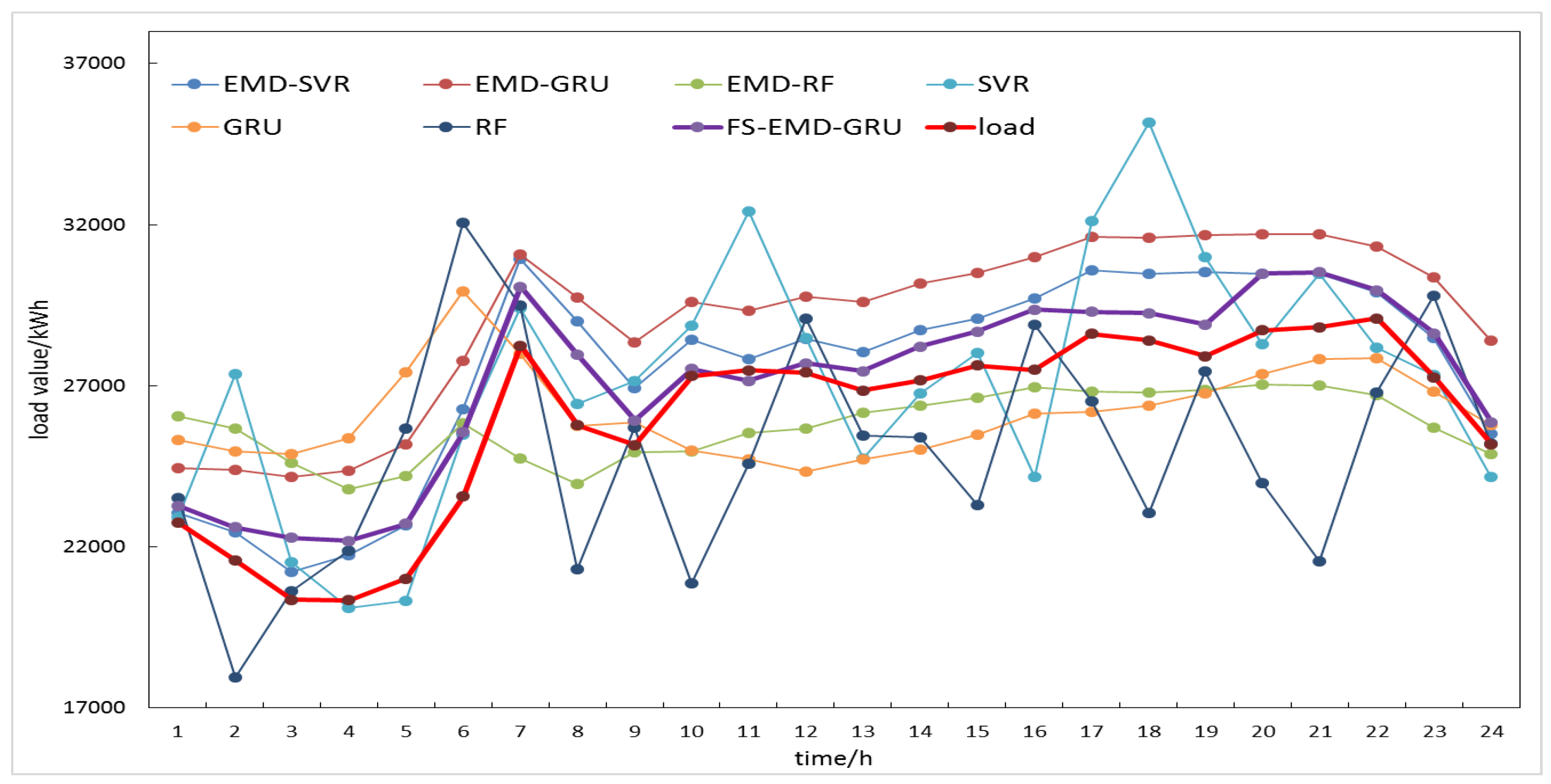
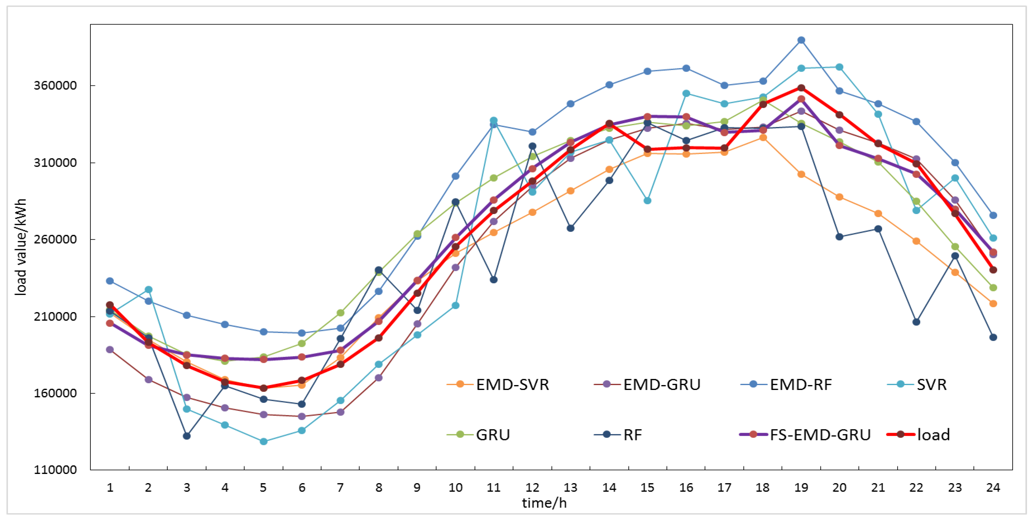
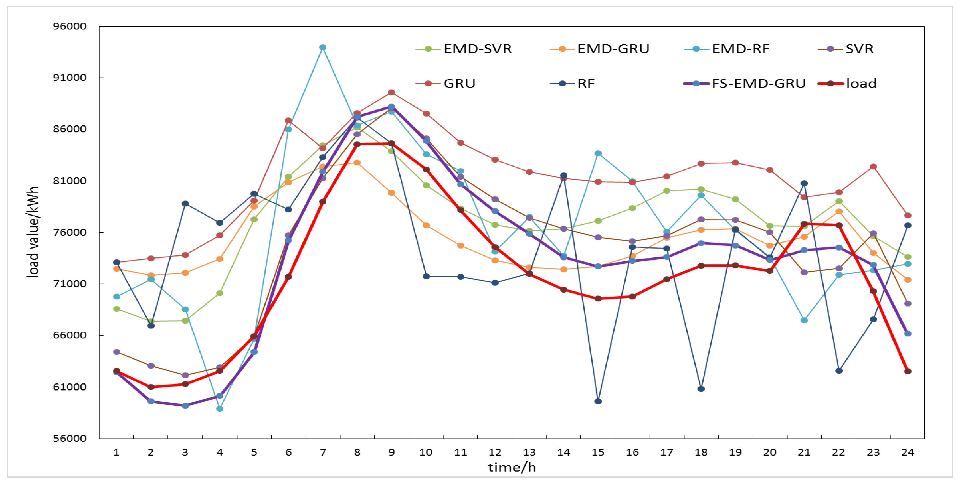
		MAPE	9.09%	6.83%	10.08%	6.52%	7.68%	9.20%	4.28%

shows the results of the prediction of 24 time points for one day in January, April, July, and October for three datasets in the U.S. The numbers in bold mean that the corresponding method has the best performance for this dataset under this performance evaluation index. It can be seen that the proposed method had the smallest average MAPE and RMSE compared to the other six methods. For example, in experiments on M_1 data set, compared to the GRU model, the MAPE of the FS-EMD-GRU model were reduced by 0.26%, 9.23%, 0.70%, and 8.14%, respectively; the RMSE of the FS-EMD-GRU model were reduced by 80.64, 3068.49, 165.65, and 2802.72, respectively; compared to the EMD-GRU model, the MAPE of the FS-EMD-GRU model were reduced by 6.08%, 5.48%, 3.80%, and 7.52%, respectively; the RMSE of the FS-EMD-GRU model were reduced by 2477.99, 1437.69, 1774.23, and 2724.98, respectively. The average MAPE of the proposed method in the M_1, M_2, and M_3 data sets were 3.10%, 4.69%, and 4.28%, respectively. Compared with the minimum average MAPE obtained by other six methods in each data set, the proposed method reduced by 2.2%, 0.8%, and 2.24%, respectively. In addition, the average RMSE of the proposed method in the M_1, M_2, and M_3 data sets were 1309.58, 13,322.47, and 4827.02, respectively. Compared with the minimum average RMSE obtained by other six methods in each data set, the proposed method reduced by 585.21, 4095.49, and 1519.85, respectively. At the same time, it could be learned that for a single prediction model, the GRU model was superior to SVR and RF in most cases, which shows that the GRU network had better performance in processing time series; the performance of the EMD-based hybrid prediction models in MAPE and RMSE were better than the single models in most cases, which showed the effectiveness of the EMD method. Figure 9, Figure 10 and Figure 11 show the comparison curves of predicted and actual values obtained by each model on the three datasets M_1, M_2 and M_3, respectively. These figures demonstrate the proposed method could better capture the trend of load change, whether in daily peak or valley.

Table 4. Comparison of the running time and memory space requirements of the EMD-GRU model and the FS-EMD-GRU model.

Dataset	Model	Running Time (s)	Memory Requirement (MB)
M_1	EMD-GRU	836.7	496.5
	FS-EMD-GRU	195.1	168.3
M_2	EMD-GRU	766.4	498.3
	FS-EMD-GRU	194.8	168.1
M_3	EMD-GRU	770.2	497.1
	FS-EMD-GRU	198.2	167.7

shows the comparison of the running time and memory space requirements of the EMD-GRU model and the FS-EMD-GRU model on the M_1, M_2 and M_3 dataset, respectively. All the models were built on a desktop PC with a 3.6 GHz Intel i7 processor and 8 GB of memory using the tensorflow frame. It was obvious that the running time and memory space of EMD-GRU model were much greater than that of FS-EMD-GRU model. Compared with the methods of establishing a prediction model for each sub-series separately, the proposed method could effectively reduce the overall complexity of the model.

Table 5. Comparison of dataset prediction results in Northwest China.

Model	MAPE	RMSE
GRU	3.16%	26,490.43
SVR	6.04%	45,568.98
RF	8.69%	68,920.11
EMD-GRU	4.87%	34,359.27
EMD-SVR	3.83%	29,982.13
EMD-RF	5.65%	43,535.79
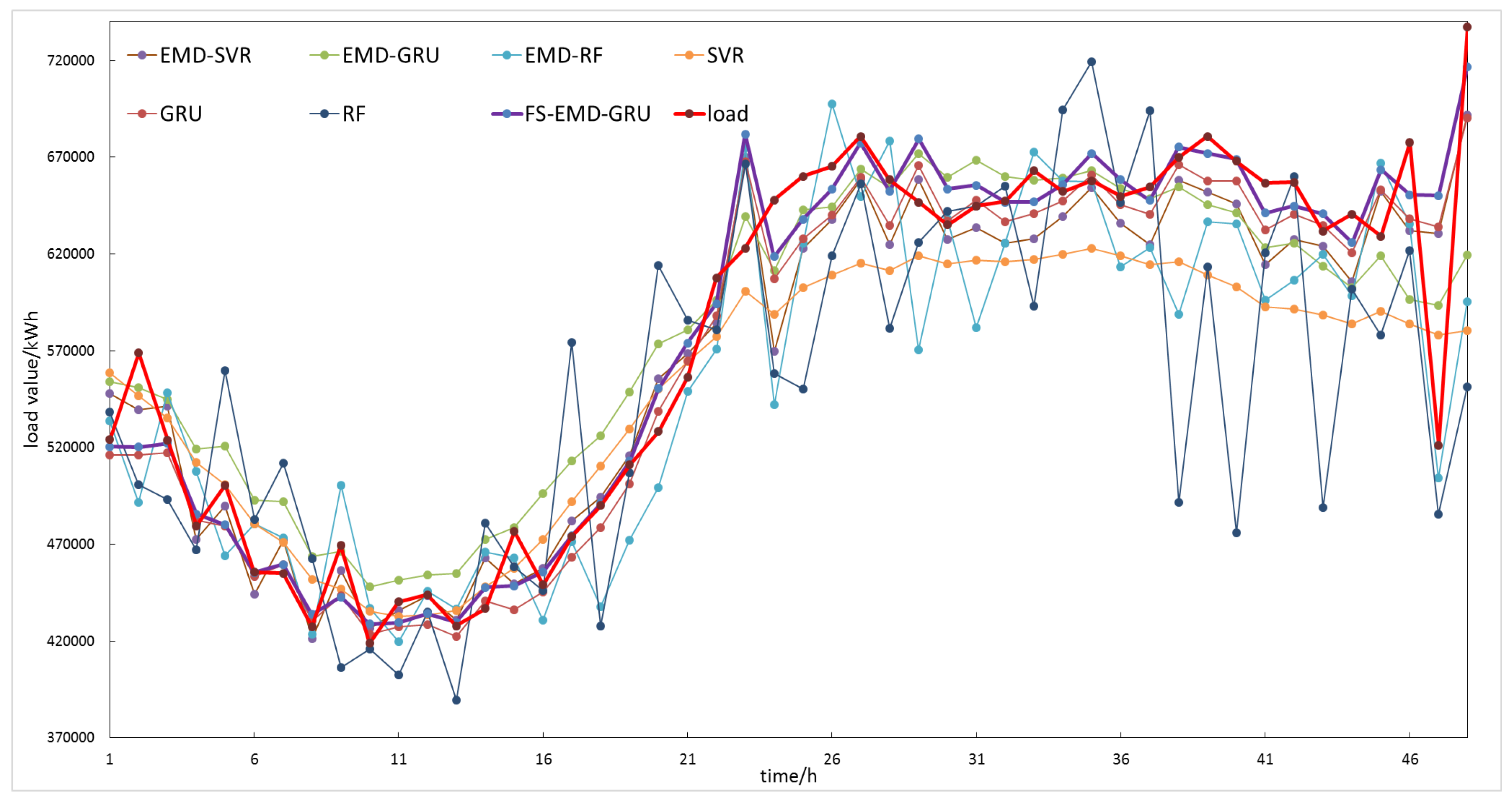
FS-EMD-GRU	2.83%	26,143.36

shows the prediction results of each model for 48 time points on a certain day in July 2017 in a region of Northwest China. It can be seen from the table that compared with the other six methods, the proposed method had the smallest MAPE and RMSE, which were 2.83% and 26,143.36, respectively. Compared with the other six methods, the minimum MAPE and RMSE decreased by 0.33% and 347.07, respectively. Figure 12 shows the comparison curves of load forecasting values and actual values of each model. It could be seen that the proposed method can better capture the trend of load change and had a better fitting effect for the load series.

5. Conclusions

This paper proposes an EMD-GRU short-term electricity load forecasting method with feature selection. Instead of establishing a forecasting model for each component decomposed by EMD, the decomposed time series components were selected by correlation analysis method. The components that were highly correlated with the original load series were selected as features and input into the GRU forecasting model together with the original load series to establish the final prediction model. Four load data sets from the U.S. Public Utilities and a region in Northwest China were used to evaluate the proposed method, and six comparison methods were used to verify the effectiveness of the proposed method. The experiment results showed that the GRU network in the deep learning method had the advantage in processing the load time series; the EMD-based hybrid prediction method was usually better than the corresponding single structure model; and the EMD-GRU prediction method with feature selection proposed in this paper had the best performance in all comparison methods.

References

- Carvallo, J.P.; Larsen, P.H.; Sanstad, A.H. Long term load forecasting accuracy in electric utility integrated resource planning. Energy Policy 2018, 119, 410–422. [Google Scholar] [CrossRef]
- Nagaraja, Y.; Devaraju, T.; Kumar, M.V. A survey on wind energy, load and price forecasting: (Forecasting methods). In Proceedings of the International Conference on Electrical, Electronics, and Optimization Techniques (ICEEOT), Chennai, India, 3–5 March 2016; pp. 783–788. [Google Scholar]
- Srivastava, A.K.; Pandey, A.S.; Singh, D. Short-term load forecasting methods: A review. In Proceedings of the International Conference on Emerging Trends in Electrical Electronics & Sustainable Energy Systems (ICETEESES), Sultanpur, India, 11–12 March 2016; pp. 130–138. [Google Scholar]
- Li, L.; Ota, K.; Dong, M. When Weather Matters: IoT-Based Electrical Load Forecasting for Smart Grid. IEEE Commun. Mag. 2017, 55, 46–51. [Google Scholar] [CrossRef]
- Ailing, Y.; Weide, L.; Xuan, Y. Short-term electricity load forecasting based on feature selection and Least Squares Support Vector Machines. Knowl. Based Syst. 2019, 163, 159–173. [Google Scholar]
- Ma, J.; Ma, X. State-of-the-art forecasting algorithms for microgrids. In Proceedings of the International Conference on Automation & Computing(ICAC), Huddersfield, UK, 7–8 September 2017; pp. 1–6. [Google Scholar]
- Chan, F.; Pauwels, L.L. Some theoretical results on forecast combinations. Int. J. Forecast. 2018, 34, 64–74. [Google Scholar] [CrossRef]
- Singh, P.; Dwivedi, P. Integration of new evolutionary approach with artificial neural network for solving short term load forecast problem. Appl. Energy 2018, 217, 537–549. [Google Scholar] [CrossRef]
- Haida, T. Regression based peak load forecasting using a transformation technique. IEEE Trans. Power Syst. 1994, 9, 1788–1794. [Google Scholar] [CrossRef]
- Khashei, M.; Bijari, M. A novel hybridization of artificial neural networks and ARIMA models for time series forecasting. Appl. Soft Comput. J. 2011, 11, 2664–2675. [Google Scholar] [CrossRef]
- Holt, C. Forecasting seasonals and trends by exponentially weighted moving averages. Int. J. Forecast. 2004, 20, 5–10. [Google Scholar] [CrossRef]
- Wang, Y.; Niu, D.; Ji, L. Short-term power load forecasting based on IVL-BP neural network technology. Syst. Eng. Procedia 2012, 4, 168–174. [Google Scholar] [CrossRef]
- Fu, Y.; Li, Z.; Zhang, H.; Xu, P. Using Support Vector Machine to Predict Next Day Electricity Load of Public Buildings with Sub-metering Devices. Procedia Eng. 2015, 121, 1016–1022. [Google Scholar] [CrossRef]
- Lahouar, A.; Ben, H.S.J. Day-ahead load forecast using random forest and expert input selection. Energy Convers. Manag. 2015, 103, 1040–1051. [Google Scholar] [CrossRef]
- Tong, C.; Li, J.; Lang, C. An efficient deep model for day-ahead electricity load forecasting with stacked denoising auto-encoders. J. Parallel Distrib. Comput. 2018, 117, 267–273. [Google Scholar] [CrossRef]
- Heigold, G.; Vanhoucke, V. Multilingual acoustic models using distributed deep neural networks. In Proceedings of the IEEE International Conference on Acoustics, Speech and Signal Processing, Vancouver, BC, Canada, 26–31 May 2013; pp. 8619–8623. [Google Scholar]
- He, K.; Zhang, X.; Ren, S. Deep Residual Learning for Image Recognition. In Proceedings of the IEEE Conference on Computer Vision and Pattern Recognition(CVPR), Las Vegas, NV, USA, 26 June–1 July 2016; pp. 770–778. [Google Scholar]
- Mocanu, E.; Nguyen, P.H.; Gibescu, M.; Kling, W.L. Deep learning for estimating building energy consumption. Sustain. Energy Grids Netw. 2016, 6, 91–99. [Google Scholar] [CrossRef]
- Kong, W.; Dong, Z.Y.; Jia, Y. Short-Term Residential Load Forecasting based on LSTM Recurrent Neural Network. IEEE Trans. Smart Grid 2017, 10, 49–53. [Google Scholar] [CrossRef]
- Rahman, A.; Srikumar, V.; Smith, A.D. Predicting electricity consumption for commercial and residential buildings using deep recurrent neural networks. Appl. Energy 2018, 201, 372–385. [Google Scholar] [CrossRef]
- Mohamed, M. Parsimonious Memory Unit for Recurrent Neural Networks with Application to Natural Language Processing. Neurocomputing 2018, 314, 48–64. [Google Scholar]
- Qiu, X.; Ren, Y.; Suganthan, P.N. Empirical Mode Decomposition based ensemble deep learning for load demand time series forecasting. Appl. Soft Comput. 2017, 54, 246–255. [Google Scholar] [CrossRef]
- Rana, M.; Koprinska, I. Forecasting electricity load with advanced wavelet neural networks. Neurocomputing 2016, 182, 118–132. [Google Scholar] [CrossRef]
- Huang, N.E.; Shen, Z.; Long, S.R. The Empirical Mode Decomposition and the Hilbert Spectrum for Nonlinear and Non-Stationary Time Series Analysis. Proc. R. Soc. Lond. A Math. Phys. Eng. Sci. 1998, 454, 903–995. [Google Scholar] [CrossRef]
- Fan, G.F.; Peng, L.; Hong, W.C. Electric load forecasting by the SVR model with differential empirical mode decomposition and auto regression. Neurocomputing 2016, 173, 958–970. [Google Scholar] [CrossRef]
- Bedi, J.; Toshniwal, D. Empirical Mode Decomposition Based Deep Learning for Electricity Demand Forecasting. IEEE Access 2018, 6, 49144–49156. [Google Scholar] [CrossRef]
- Lahmiri, S. Comparing Variational and Empirical Mode Decomposition in Forecasting Day-Ahead Energy Prices. IEEE Syst. J. 2017, 11, 1907–1910. [Google Scholar] [CrossRef]
- Da Silva, I.D.; das Chagas Moura, M.; Lins, I.D.; Droguett, E.L.; Braga, E. Non-Stationary Demand Forecasting Based on Empirical Mode Decomposition and Support Vector Machines. IEEE Latin Am. Trans. 2017, 15, 1785–1792. [Google Scholar] [CrossRef]
- Cho, K.; Van Merrienboer, B.; Gulcehre, C. Learning phrase representations using RNN encoder-decoder for statistical machine translation. In Proceedings of the 2014 Conference on Empirical Methods in Natural Language Processing (EMNLP), Doha, Qatar, 25–29 October 2014. [Google Scholar]
- Jiao, R.; Zhang, T.; Jiang, Y. Short-Term Non-residential Load Forecasting based on Multiple Sequences LSTM Recurrent Neural Network. IEEE Access 2018, 6, 59438–59448. [Google Scholar] [CrossRef]
- Zheng, J.; Xu, C.; Zhang, Z. Electric load forecasting in smart grids using Long-Short-Term-Memory based Recurrent Neural Network. In Proceedings of the 2017 51st Annual Conference on Information Sciences and Systems (CISS), Baltimore, MD, USA, 22–24 March 2017; pp. 1–6. [Google Scholar]
- Cho, K.; Van Merrienboer, B.; Bahdanau, D. On the Properties of Neural Machine Translation: Encoder-Decoder Ap-proaches. In Proceedings of the of SSST-8, Eighth Workshop on Syntax, Semantics and Structure in Statistical Translation, Doha, Qatar, 25 October 2014. [Google Scholar]
- Yuan, Y.; Tian, C.; Lu, X. Auxiliary Loss Multimodal GRU Model in Audio-visual Speech Recognition. IEEE Access 2018, 6, 5573–5583. [Google Scholar] [CrossRef]
- Xu, J.; Tang, B.; He, H. Semisupervised Feature Selection Based on Relevance and Redundancy Criteria. IEEE Trans. Neural Netw. Learn. Syst. 2017, 28, 1974–1984. [Google Scholar] [CrossRef] [PubMed]
- Hong, T.; Pinson, P.; Fan, S. Global Energy Forecasting Competition 2012. Int. J. Forecast. 2014, 30, 357–363. [Google Scholar] [CrossRef]
- Mu, Y.; Liu, X.; Wang, L. A Pearson’s correlation coefficient based decision tree and its parallel implementation. Inf. Sci. 2018, 435, 40–58. [Google Scholar] [CrossRef]
- Salah, B.; Ali, F.; Ali, O. Optimal Deep Learning LSTM Model for Electric Load Forecasting using Feature Selection and Genetic Algorithm: Comparison with Machine Learning Approaches? Energies 2018, 11, 1636. [Google Scholar]
- Kim, S.H.; Lee, G.; Kwon, G.Y. Deep Learning Based on Multi-Decomposition for Short-Term Load Forecasting. Energies 2018, 11, 3433. [Google Scholar] [CrossRef]
Figure 1.
Example of one month load decomposition in a public utility sector in the U.S.
Figure 2.
The basic structure of GRU.
Figure 3.
Structure of the proposed empirical mode decomposition-gated recurrent unit (EMD-GRU) model with feature selection.
Figure 4.
Partial load time series corresponding to four datasets.
Figure 5.
M_1 load series decomposition results.
Figure 6.
M_2 load series decomposition results.
Figure 7.
M_3 load series decomposition results.
Figure 8.
C_1 load series decomposition results.
Figure 9.
Comparisons of load forecasting results for a certain day in April 2006 of M_1 dataset.
Figure 10.
Comparisons of load forecasting results for a certain day in July 2006 of M_2 dataset.
Figure 11.
Comparisons of load forecasting results for a certain day in April 2006 of M_3 dataset.
Figure 12.
Comparisons of load forecasting results for a certain day in July 2017 in a region of Northwest China.