Single and Multi-Sequence Deep Learning Models for Short and Medium Term Electric Load Forecasting


1
Department of Computer Science and Software Engineering, UAE University, 15551 Al Ain, UAE
2
Department of Software Engineering and IT, Ecole de Technologie Superieure, Montréal, QC H3C 1K3, Canada
*
Author to whom correspondence should be addressed.
Energies 2019, 12(1), 149; https://doi.org/10.3390/en12010149
Submission received: 28 October 2018
/
Revised: 23 November 2018
/
Accepted: 26 November 2018
/
Published: 2 January 2019
Abstract
:Time series analysis using long short term memory (LSTM) deep learning is a very attractive strategy to achieve accurate electric load forecasting. Although it outperforms most machine learning approaches, the LSTM forecasting model still reveals a lack of validity because it neglects several characteristics of the electric load exhibited by time series. In this work, we propose a load-forecasting model based on enhanced-LSTM that explicitly considers the periodicity characteristic of the electric load by using multiple sequences of inputs time lags. An autoregressive model is developed together with an autocorrelation function (ACF) to regress consumption and identify the most relevant time lags to feed the multi-sequence LSTM. Two variations of deep neural networks, LSTM and gated recurrent unit (GRU) are developed for both single and multi-sequence time-lagged features. These models are compared to each other and to a spectrum of data mining benchmark techniques including artificial neural networks (ANN), boosting, and bagging ensemble trees. France Metropolitan’s electricity consumption data is used to train and validate our models. The obtained results show that GRU- and LSTM-based deep learning model with multi-sequence time lags achieve higher performance than other alternatives including the single-sequence LSTM. It is demonstrated that the new models can capture critical characteristics of complex time series (i.e., periodicity) by encompassing past information from multiple timescale sequences. These models subsequently achieve predictions that are more accurate.
1. Introduction
Electrical energy must be consumed as soon as it is produced since it cannot be stored. Thus, its demand and supply must be carefully balanced through accurate load forecasting [1]. Moreover, the success of energy domain activities like load scheduling, power system planning and economical operation of power plants is crucially depending on the accuracy of load forecasting for the short and medium term horizons. One way of achieving accurate load forecasting is time series analysis. The purpose of such a technique is to carefully consider the past observations in order to identify data patterns that best describe the inherent structure buried in the series and capture the underlying data generation process [2]. The autoregressive integrated moving average algorithm (ARIMA) is a well-known statistical approach commonly used for time series modeling to accurately predict short-term temporal structures. Similarly, the autoregressive (AR) model provides adequate representation of the data generation mechanism based on time series. These techniques use the assumption that time series data (readings) are only linearly dependent on some past readings of the same time series. However, for long and complex time series, the forecasting performance of these techniques drops since their derived models assume linear relationships and stationary properties of the time series.
Electric load profile for a large metropolitan follows complex cyclic and seasonal patterns which are related to industrial production calendar, weather impacts and human activities. Non-linear models using the past history usually perform better than simple linear models like moving average (MA) and autoregressive integrated moving average (ARIMA) [3]. In general, several approaches of electric load forecasting using traditional statistical and machine learning techniques have been proposed to improve the accuracy forecasting, however the need of more robust load forecasting models is still a high priority [4].
In this direction, deep learning approaches have recently gain significant attention of many researchers and have showed tremendous progresses in many domains like acoustic modeling, natural language processing, and image recognition [5,6,7]. These deep layered structures increase feature abstraction capability and allow complex non-linear patterns modeling. In particular, recurrent neural network (RNN), which is a deep learning architecture designed specifically to operate over sequential time series data and LSTM is a variation RNN originally developed by Hochreiter et al. [8]. It allows preservation of the weights that are propagated forward and backward through layers. Similarly gated recurrent networks (GRU) is another variation of standard RNN introduced by Cho, et al. in [9] which like LSTMs overcome the problem of vanishing gradient to model long term sequences. LSTM and GRUs are attractive schemes for modeling sequential data as they encode contextual information from past inputs thanks to their ability to learn complex non-linear patterns and automatically extracting relevant features. Despite their attractiveness, the applications of these deep learning models are relatively rare and mostly concern computer-related domains. To the best of our knowledge, we were among the first who have proposed a time series analysis based on LSTM deep learning model to predict short and medium electric loads [10]. Although, it performed better than alternative machine learning approaches, the proposed LSTM forecasting model revealed a lack of validity and therefore was unable to sustain high out-of-sample performance. This is because it neglects the complex electric load characteristics exhibited by time series, like periodicity, data frequency, trends, levels, structural breaks and calendar effects. In particular, the complex daily, weekly, monthly and yearly patterns of electric load are not included as input to the previous LSTM based forecasting model. It rather considers only one single sequence of past loads as input to predict the short and medium term electrical loads. Accordingly, the previously proposed model ignores important domain knowledge that might have an impact on the forecasting validity and robustness.
In this work, we propose a load-forecasting model based on enhanced-LSTM that explicitly considers the periodicity characteristics of the electric load while using multiple sequences of relevant inputs time lags. In order to incorporate the past electric load readings that will be used by multi-sequence LSTM, an autoregressive model is developed together with an autocorrelation function (ACF) to regress consumption and identify the time lags that are most relevant to the multi-sequence LSTM. For the sake of comparison and validation, two variations of deep neural networks, LSTM and GRU are developed for both single and multi-sequence time-lagged features. Machine learning like multi-layer perceptron, boosting and bagging ensemble trees techniques are implemented in order to be compared to our proposed approach. France Metropolitan’s electricity energy consumption data is used as test bed. Experimental results show that multi sequence LSTM and GRU forecasting models significantly outperform the other alternative machine learning techniques.
The rest of the paper is organized as follows: Section 2 summarizes the literature on the evolution of electrical load forecasting and underlines the differences between our current and previous proposals. While Section 3 provides a brief description of LSTM, GRU and the state-of-the-art machine learning benchmarks, Section 4 introduces the methodology of the proposed approach along with an exploratory data analysis. Section 5 describes the experimental results and the performance evaluation. Section 6 is dedicated to our models’ validation over the short and medium horizons, and provides a discussion on threat to validity. Finally, Section 7 draws the conclusions and presents suggestions for future work.
2. Literature Review
Load forecasting has been widely studied for different horizons over the last decades. Especially, the short-term horizon has attracted considerable research effort [11,12,13,14], where the aim was always to improve the performance of forecasting though efficient use of modeling techniques. Simultaneously, several works on forecasting classification have identified two main categories of forecasting methods, namely, engineering methods and data driven methods. In the past energy modeling was mostly based on engineering approaches using dedicated building energy simulation tools. These approaches were time consuming and required detailed domain expertise as well as significant amount of information regarding the structural, metallurgical and geometric properties of the building [4]. Nowadays, proliferation of smart meters, various low cost sensors and BAS has enabled availability of large amount of electricity consumption data that has supported more and more researchers to use data driven approaches for modeling and analysis. Data driven methods, rely on historical data collected from tracking the energy consumption of previous episodes. They are very attractive Artificial Intelligence (AI) methods, however little is known about their forecasting ability out of sample. Indeed, their accuracy decrease when applied in new circumstances. Unfortunately, the ability of generalization of AI forecasting models remains problematic [11].
Electricity demand forecasting plays a key role for power companies as they need to develop long and short term strategies, in particular short-term load forecasting (STLF) has attracted considerable attention in smart grids and buildings. In fact, several works ranging from classical time series analysis to recent machine learning approaches have been carried out on STLF [14,15,16,17,18,19]. Yukseltan, et al. used sinusoidal variations as input features to a linear regression model to predict electricity demand over daily and weekly horizons reporting a 3% MAPE for Turkish power market [20]. Zhang et al. developed a SVR model to predict daily and half hourly energy consumption. The proposed models exhibit a lower MAPE for both the daily dataset and half-hourly dataset using only the time variable and its lagged values as their input [21].
Ensemble models have been successfully used for load forecasting as it performs better than single estimators. They decrease variance of a single estimate as they combine several estimates from different models resulting in higher prediction stability. Well-known approaches for homogeneous ensemble learning like boosting and bagging were used in many works. For example, Papadopoulos and Karakatsanis developed four estimation models; two of which are statistical time series and the other two are ensemble models namely random forest and gradient boosting regression trees for 24-h ahead load forecast [22]. Dudek proposed a random forest model for short term load forecast using time series data with multiple seasonal variations [23]. The random forest performed better than ARIMA, exponential smoothing and ANN. Similarly, Wang et al. proposed a hybrid model integrating discrete wavelet transform and XGBoost for electricity consumption forecast [24]. The derived model outperforms the other hybrid models that integrated discrete wavelet transform with support vector regression, ANN and unitary XGBoost.
Due to the elastic configurations of ANN structures with more than one hidden layer, deep neural networks (DNN) are attracting many researchers. Hossen et al. used a multi-layered deep neural network for the Iberian electric market data for day ahead load forecast [25]. For weekend and weekday forecast, various activation functions were tested to achieve a lower MAPE. He used a combination of convolutional neural network for feature extraction from historical load data and recurrent neural network to learn patterns for day ahead hourly load consumption [26]. Several strong baselines models including linear regression, Support Vector Regression (SVR), a DNN with three hidden layers were also used. A parallel configuration of ANN and RNN reported the lowest MAPE.
Zheng et al. [27] used LSTM neural network along with similar days selection and empirical mode decomposition to forecast short-term electric loads. This is the closest work to our previously proposed approach [10], but it reveals many technical differences. Feature importance was determined using XGBoost and k-means was employed for similar days clustering. The approach improved LSTM predictive accuracy. Machine-learning models, in particular the late deep learning, have the potential of performing better than traditional time series analysis and regression approaches [10]. However, there is still a crucial need for improvement to better model non-linear energy consumption patterns. The improvement is associated with high accuracy and stability of prediction especially for the medium term forecasting. Henceforth, in our recent work, we have demonstrated that trained deep learning model on time series data derives more accurate forecasting outputs than those obtained with a shallow structure [10]. We proved that optimal LSTM-RNN behaves similarly in the context of electric load forecasting for both the short-and-medium horizon with high accuracy achievement. In particular, our approach was compared with the machine learning benchmarks including ensemble models and several linear and non-linear models optimized with hyperparameter tuning. However, the complex daily, weekly, monthly and yearly patterns of electric load are not fully encompassed in the input of our previous LSTM based forecasting model. It rather considers one single sequence of past loads as inputs to predict the short and medium term electrical loads. Accordingly, the previous proposed model is omitting an important domain knowledge that would be critical for the forecasting validity and robustness.
In this work, we propose a load-forecasting model based on enhanced-LSTM that explicitly encompasses the periodicity characteristic of electric load while using multiple sequences of relevant inputs time lags. In order to select the past-load records that will be used by multi-sequence LSTM, an autoregressive model is developed together with an autocorrelation function to regress consumption and identify the time lags that are most relevant to the multi-sequence LSTM. Our new approach differs from other deep learning models including our previous LSTM [10] is the following aspects:
- (i)
- We train LSTM and GRU deep learning models with single and multiple time scale sequences. This will allow capturing the dynamic features in longer sequences to accurately forecast aggregate electric load while targeting predictions that are robust against time variations.
- (ii)
- We compare the LSTM and GRU models with ANN, boosting and bagging decision trees ensemble models in both single and multiple time scale sequences. The best performing model is selected for our benchmark.
3. Background
This section provides a background on LSTM and GRU RNNS and briefly describes the benchmark ensemble trees models as well as the used performance metrics of evaluation.
3.1. From RNN to LSTMs and GRUs
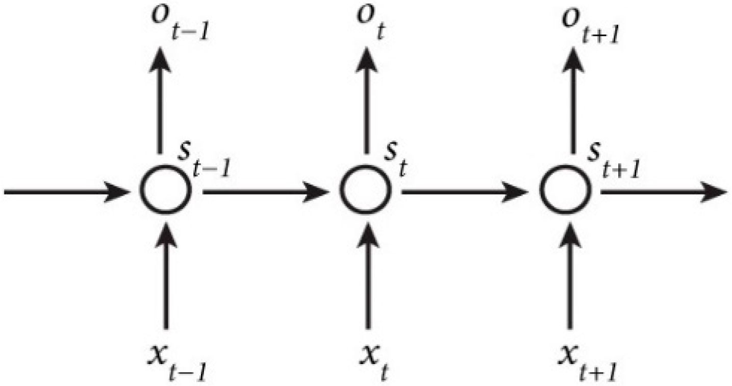
A Recurrent Neural Network utilizes sequential information in which the output depends not only on the current inputs but also on the previous inputs. They are called recurrent because the data is similarly processed for every element in the data sequence. Because of their internal memory, RNN’s can remember important information about their inputs and thus preferred for time series data. However due to vanishing gradient problem, RNNs model stops the learning process as the values of gradient become too small.
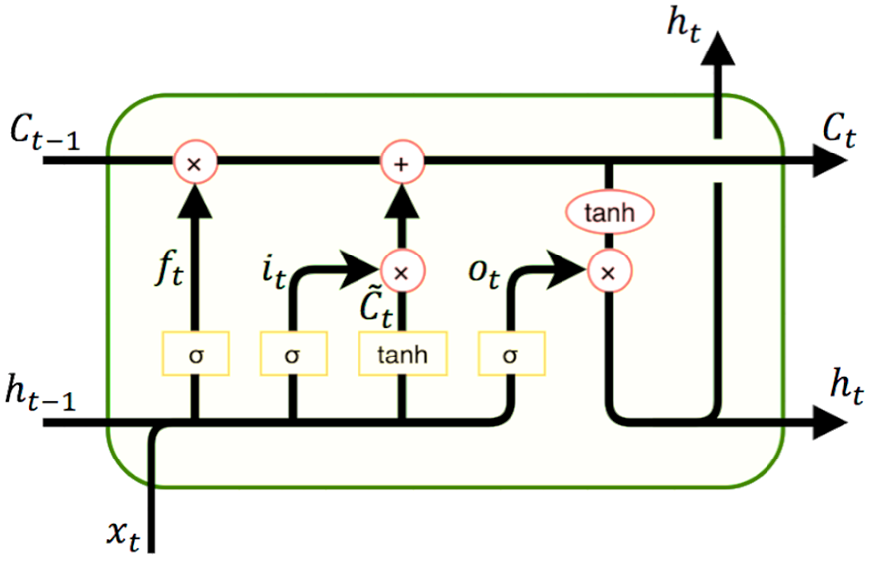
Figure 1 depicts an unrolled RNN configuration on the input sequence, where xt is the input and st is the hidden state at time step t, which is the memory of the network. Standard RNNs are affected by vanishing gradient problem, as the gradients tends to get smaller and smaller as we move backward in the network. As a result, neurons in the earlier layers learn very slowly as compared to the neurons in the later layers in the hierarchy. LSTMs and GRUs were designed to overcome this difficulty of gradient propagation. They introduce input, forget and output gates which determine addition of new information to cell state, deletion of less important information from memory and output gate that decides what to output from memory. Figure 2 (reported in ([28]) shows the information flow and the set of gates within the LSTM cells.
Gates in LSTM cell reduce the risk of vanishing gradients problem supporting learning of long-term dependencies [29]. This gating mechanism enables the LSTM cell a lot of control over what it remembers and forgets over time, allowing efficient management of its internal cell memory. LSTM models its input sequence {x1, x2, ..., xn} using recurrence function as depicted hereafter:
where xt is the input at time t, and ht is the hidden state. Gates are introduced into the recurrence function f in order to solve the gradient vanishing or explosion problem. States of LSTM cell are computed as follows:
where it, ft and ot are, respectively, the input, the forget and the output gates, the W’s and the b’s are the parameters (weights and biases) of the LSTM unit, and the current and the new candidate cell state are respectively noted as Ct and . Equations (2)–(4) are expressing three sigmoid functions for it, ft and ot gates. Given the input xt and the previous output ht−1, the three gates will block or pass the signal. In particular, if the gate is 0, then the signal is blocked. The forget gate ft determines the previous output ht−1 that are allowed to pass the gate. The input gate it decides on the input to update the cell state. The output gate ot decides what will be the output based on the cell state. The transfer function in Equation (6) calculates the new cell state Ct using the old cell state Ct−1. The new candidate values of memory cell and the output of current LSTM block ht are computed using hyperbolic tangent function defined respectively by the Equations (5) and (7). At every time step, the two states and ht are automatically transferred to the next cell. The weights W’s and biases b’s are learnt while minimizing the differences between the LSTM outputs and the actual training samples.
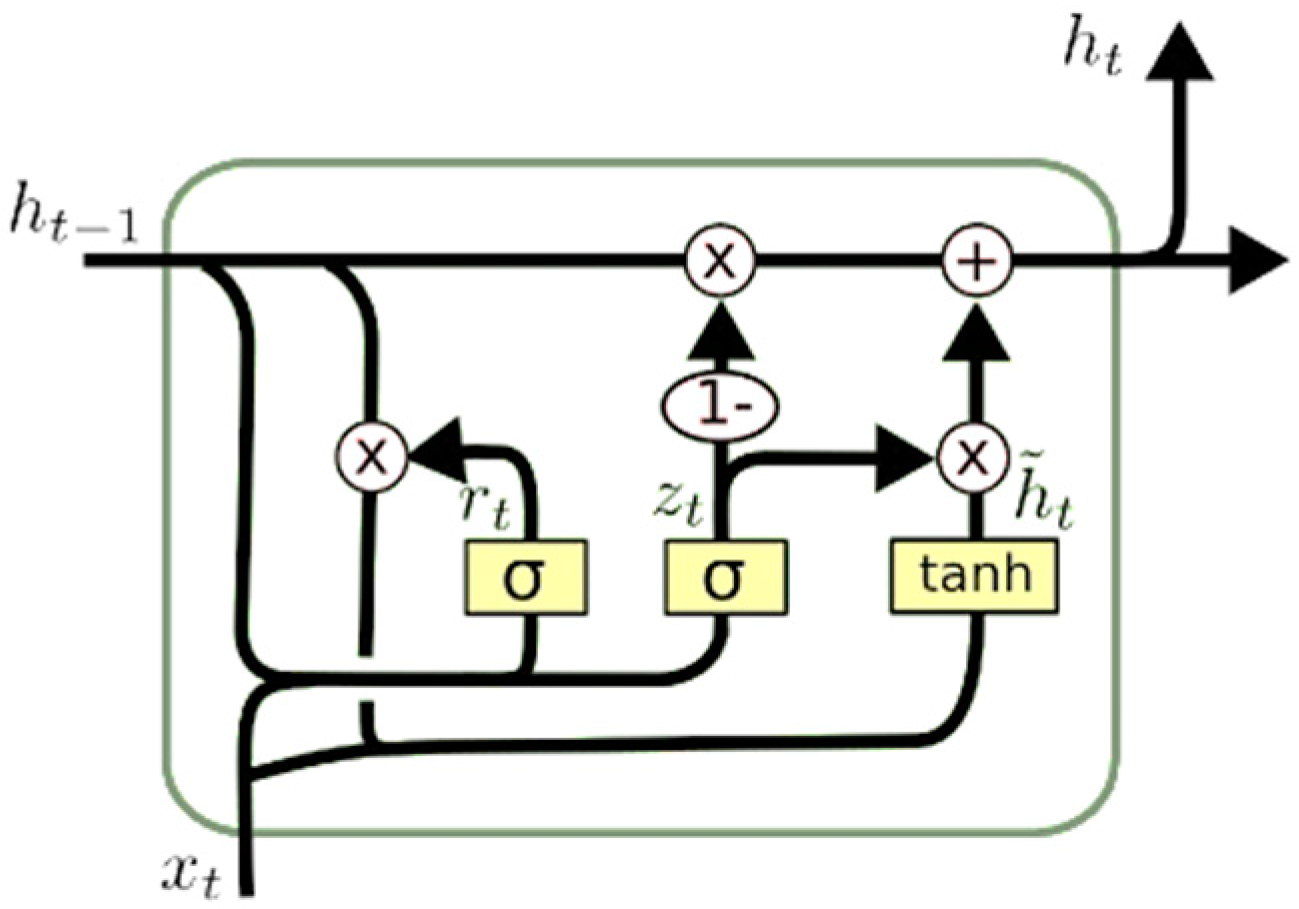
GRU is a famous variant of the LSTM; its structure is similar to a LSTM cell but with only two gates; update (combination of forget and input gates) and reset gates. The model is simpler and often computationally faster than standard LSTM models [30] as shown in Figure 3 (adopted from [28]). Like LSTM, it overcomes vanishing gradient problem and due to simpler internal structure, it is faster to train as fewer computations are required for updating hidden state. Carefully trained GRU can perform extremely well in complex modeling situations.
Update gate, reset gate and cell states for GRU are computed using the following equations:
3.2. Ensemble Approaches
Tree-based ensemble approaches, namely bagging and boosting, are used in various load-forecasting tasks and proved to be highly effective in modeling complex electricity consumption patterns [31]. Ensemble trees are effectively used for prediction tasks as they combine multiple predictions from several trees to overcome accuracy of simple prediction and avoid possible overfit. The main idea behind ensembles is that a group of weak learners come together to form a strong learner. Boosting is an ensemble technique where new models are added sequentially to correct errors made by previous models until no further improvements can be made. XGBoost, an improved version of the gradient boosted machine algorithm, provides fast computational speed and improved model performance. It allows building more stable base models with low chances of overfitting. Likewise, gradient boosting and extreme gradient boosting belong to boosting category. Commonly used bagging ensemble models are random forest and extremely randomized trees. Random forest uses a random subset of data as well as random selection of features for growing trees. Extra trees model work by random selection of both the features and cut-point choice while splitting a tree node.
3.3. Performance Metrics for Evaluation
Root mean squared error (RMSE), mean absolute error (MAE) and coefficient of variation RMSE (CVRMSE) would be used to evaluate forecast accuracy of the time series models [32]. Coefficient of variation RMSE is the root mean square error normalized to the mean of measured values. It is a dimensionless measure that quantifies the expected normalized prediction error and is a good measure of accuracy. A high CV score indicates that a model has a high error range. MAE measures the average magnitude of the forecasting errors, without considering their direction. RMSE which penalizes larger error terms, is the square root of the mean squared difference between the statistical estimate of the parameter and actual observed value. MAPE will be used to assess the performance of the forecasting models with other references. The error measures are defined using the following equations:
where is the predicted, yi is the actual, ȳ is the average energy consumption and N is the number of data points.
4. Forecasting Methodology
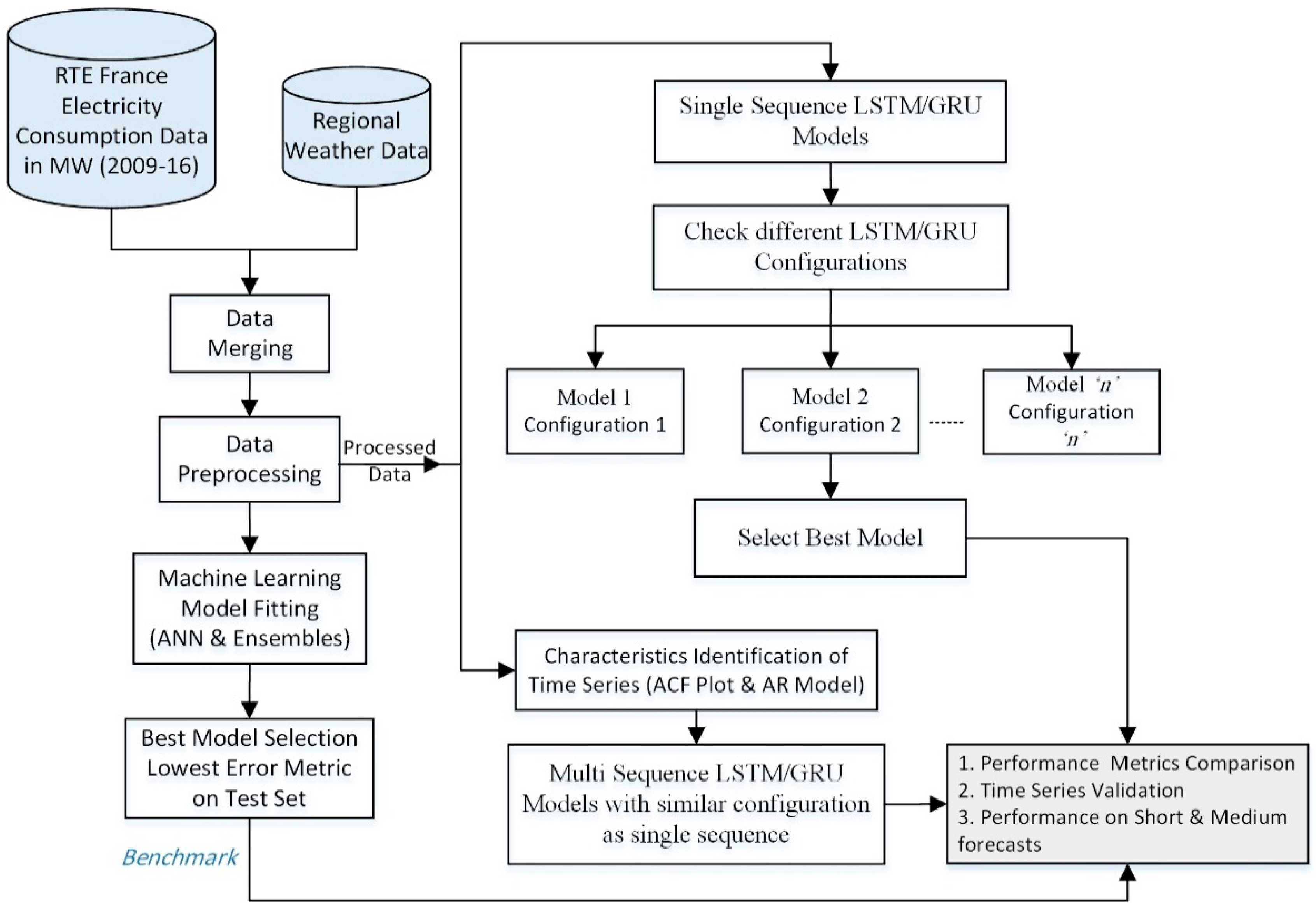
The proposed methodology for short and medium-term load forecasting using machine learning and deep learning models is depicted in Figure 4. Our model focuses on building accurate and robust predictions using multi-sequence timescale features. Half-hourly electricity consumption data spanning a period of nine years is merged with meteorological variables such as temperature, humidity and wind speed. After merging, data preprocessing is performed to check null and missing values in addition to outlier identification. Data scaling standardizes the range of variables. A training/test split is performed to split the data for model training and testing while maintaining the temporal order. The prepared data can then be used for machine leaning, single and multi-sequence LSTM and GRU deep models. The machine learning models that would be used for comparison with our approach comprise ensemble and ANN models as depicted in Figure 4. Best performing model among these machine-learning models giving the lowest forecasting error would be selected as the benchmark for comparison with single and multi-sequence models. We use an ACF plot and autoregressive model to identify the characteristics of time series like the most significant lags. Several configurations of the LSTM and GRU models are then trained. These configurations include single and multiple lags as inputs with different lengths, neural network architecture, training epochs, batch size and type of optimizer etc. The best performing configurations of LSTM and GRU are determined empirically after training several single and multi-sequence models. Finally, the LSTM and GRU model performances are compared to the machine learning benchmark. The model validation using time series split, sliding window approach and on different short and medium term horizons of the proposed model is carried out.
4.1. Exploratory Data Analysis
We have used RTE power consumption data set [33], which comprises half-hourly electrical consumption in megawatts for a period of 09 years for a metropolitan power system in France. The power consumption dataset ranges from January 2008 until December 2016.
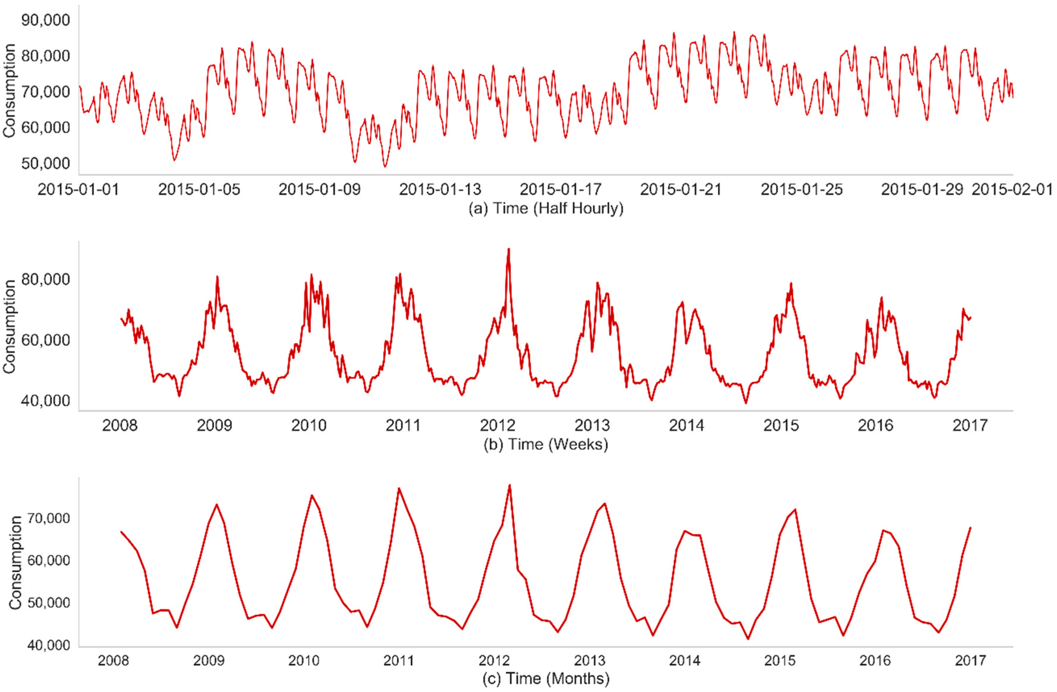
As depicted in the Figure 5, the daily, the weekly and the monthly load profiles exhibit characteristics like cyclicity and seasonality of the aggregated electricity consumption. Such characteristics are obviously compatible with the electricity domain knowledge that reflects the cyclic and seasonal behaviors of electricity consumers.
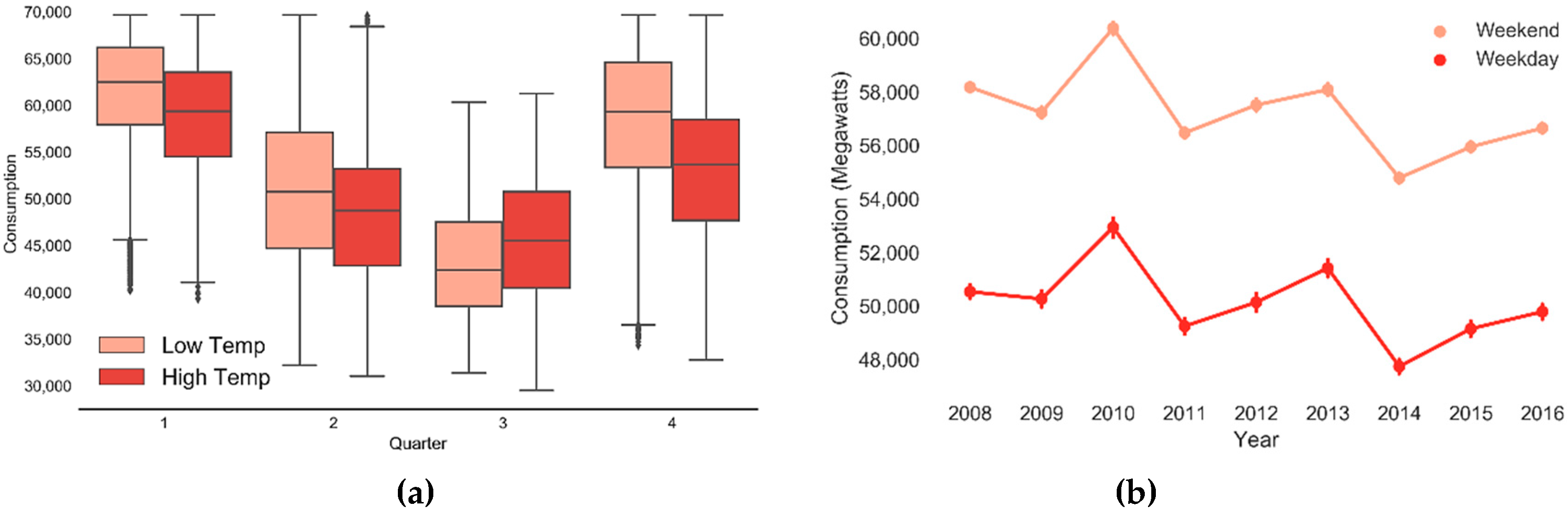
In Figure 6, the box plot of quarterly load across all years with respect to high and low temperatures shows a decline in the consumption during the second and the third quarters, and an increase during the first and the fourth quarters. In addition, the holidays and weekends can affect the electricity usage; thus weekend-weekday indicator can be used as a potential feature in forecasting models as it allows differentiating different consumption magnitudes. The consumption magnitude is quite different for weekend and weekdays across all years since user appliances usage behaviors can differ during weekends as shown in the factor plot in Figure 6b.
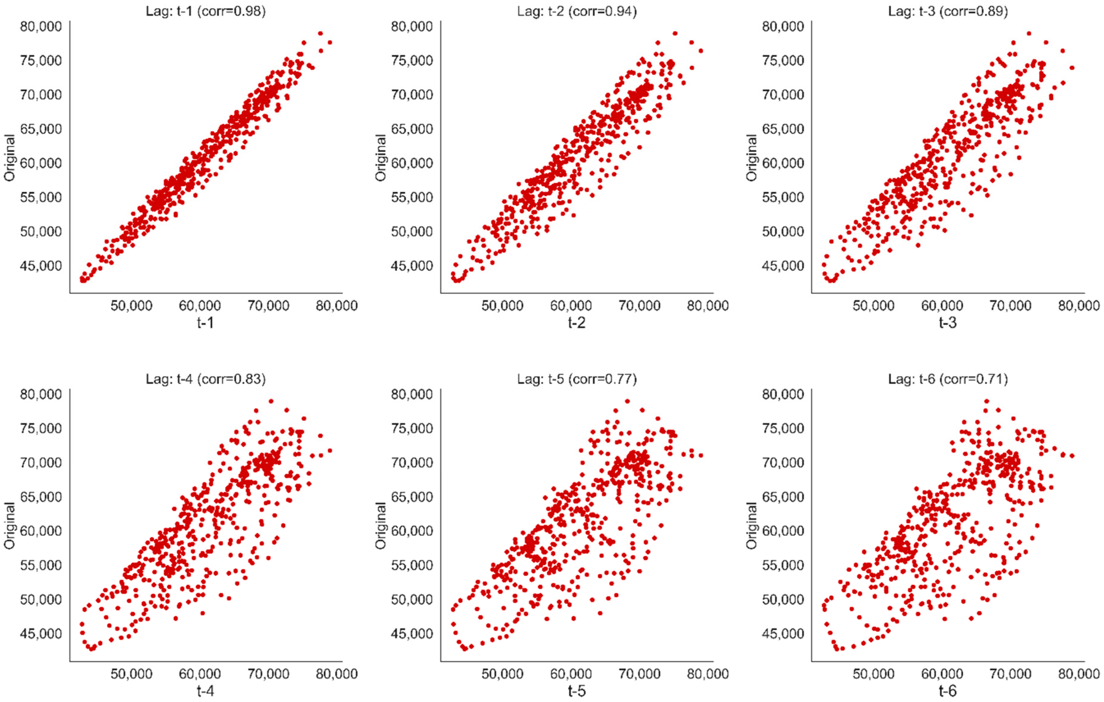
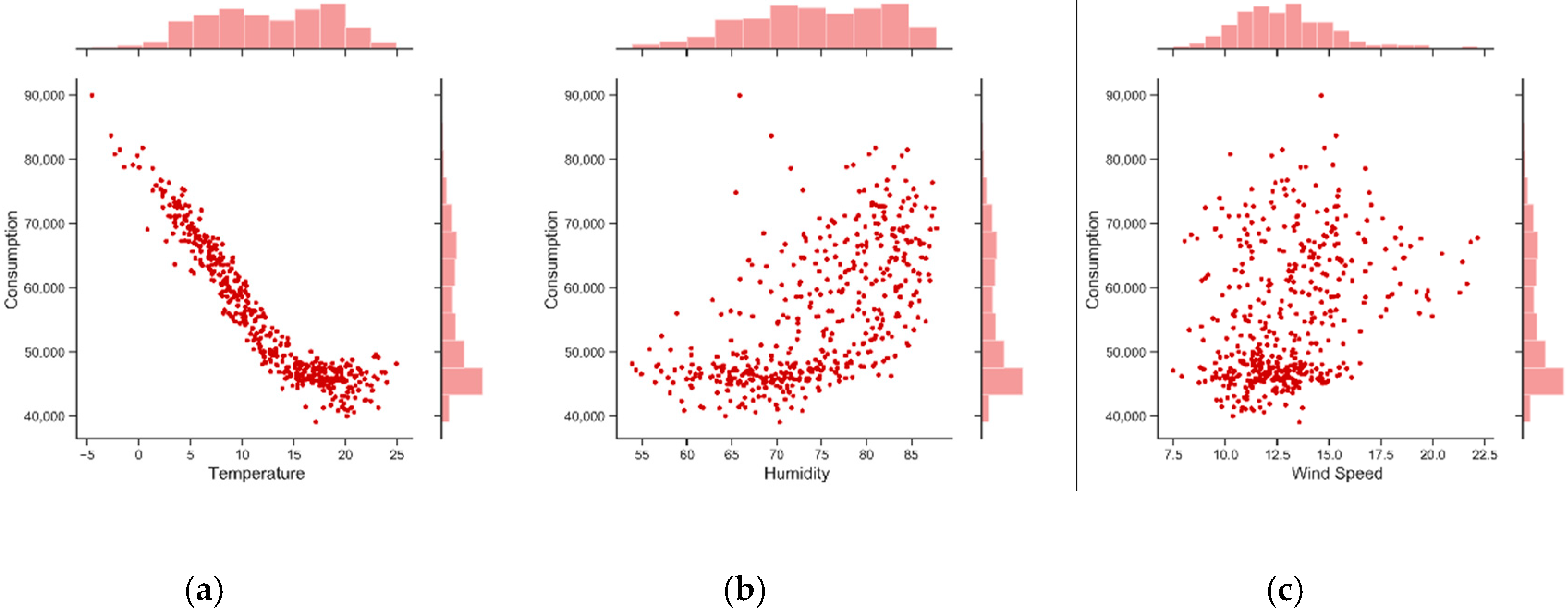
The correlation plot in Figure 7 indicates a high correlation of electricity consumption with its previous time lags suggesting that lags might be useful predictors of the dependent variable, i.e., electricity consumption. The joint plot of weather variables depicted in Figure 8, shows that temperature has a high negative correlation of 0.94 with consumption while humidity and wind speed have, respectively, low correlations of 0.61 and 0.32. The correlation between the consumption and the temperature is explained by the cooling nature of the load being analyzed.
4.2. Selecting Machine Learning Benchmark Model
As explained in the methodology, after data preprocessing we need to benchmark models. The benchmarking allows comparing our models with the existing ones and empirically rank different algorithms according to certain performance criteria. Hence, we start modeling by fitting a multi-layer perceptron (MLP) model representing the most basic form of neural networks for multivariate statistical analysis. Afterwards, we will build four ensemble models—two bagging and two boosting models—as shown in Figure 9. The best performing model will be selected as benchmark. The data is split into training and test set data while maintaining the temporal order of observations. Since our dataset is fairly large comprising more than 150 thousand records, training and tests partitions would therefore adequately represent the original load forecasting problem.
The input of these models are time lags, weather variables such as temperature, humidity, and wind speed, in addition to weekend-weekday indicator, month number and quarter. By using lags of variables, regression model allows learning from various time moments in the recent history. All the models use mean squared error as the loss function for optimization purpose. Three performance metrics are used to evaluate all the trained models’ achievements on the same testing dataset. The results are shown in Table 1.
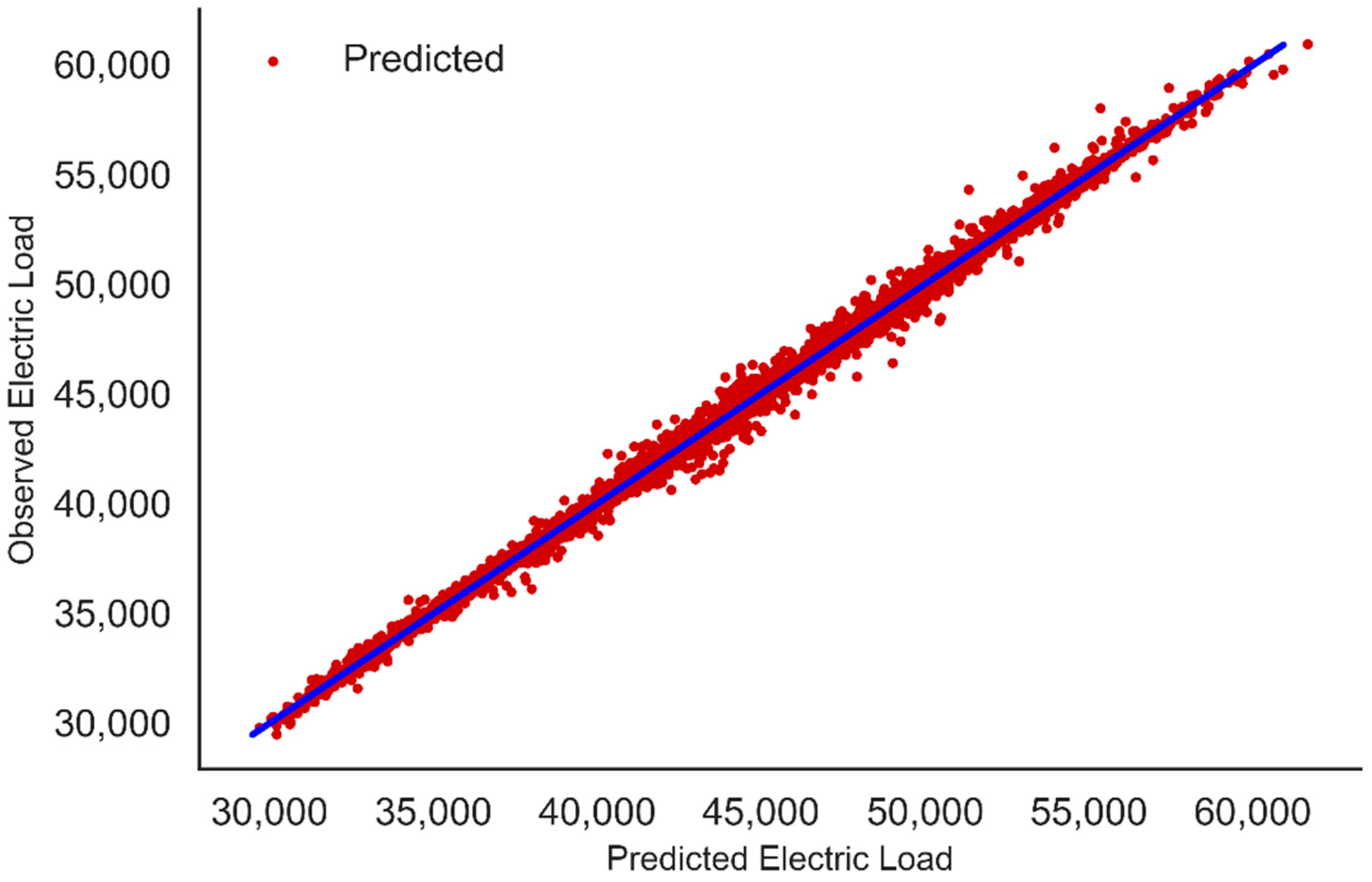
Given its highest performance, the boosting model XGBoost is used as a benchmark model. Figure 10 shows a high agreement, at different load scales, between the observed load and the load predicted by the XGBoost model. For a perfect model all the points will lie on the diagonal blue line.
Checking Overfitting for XGBoost Model
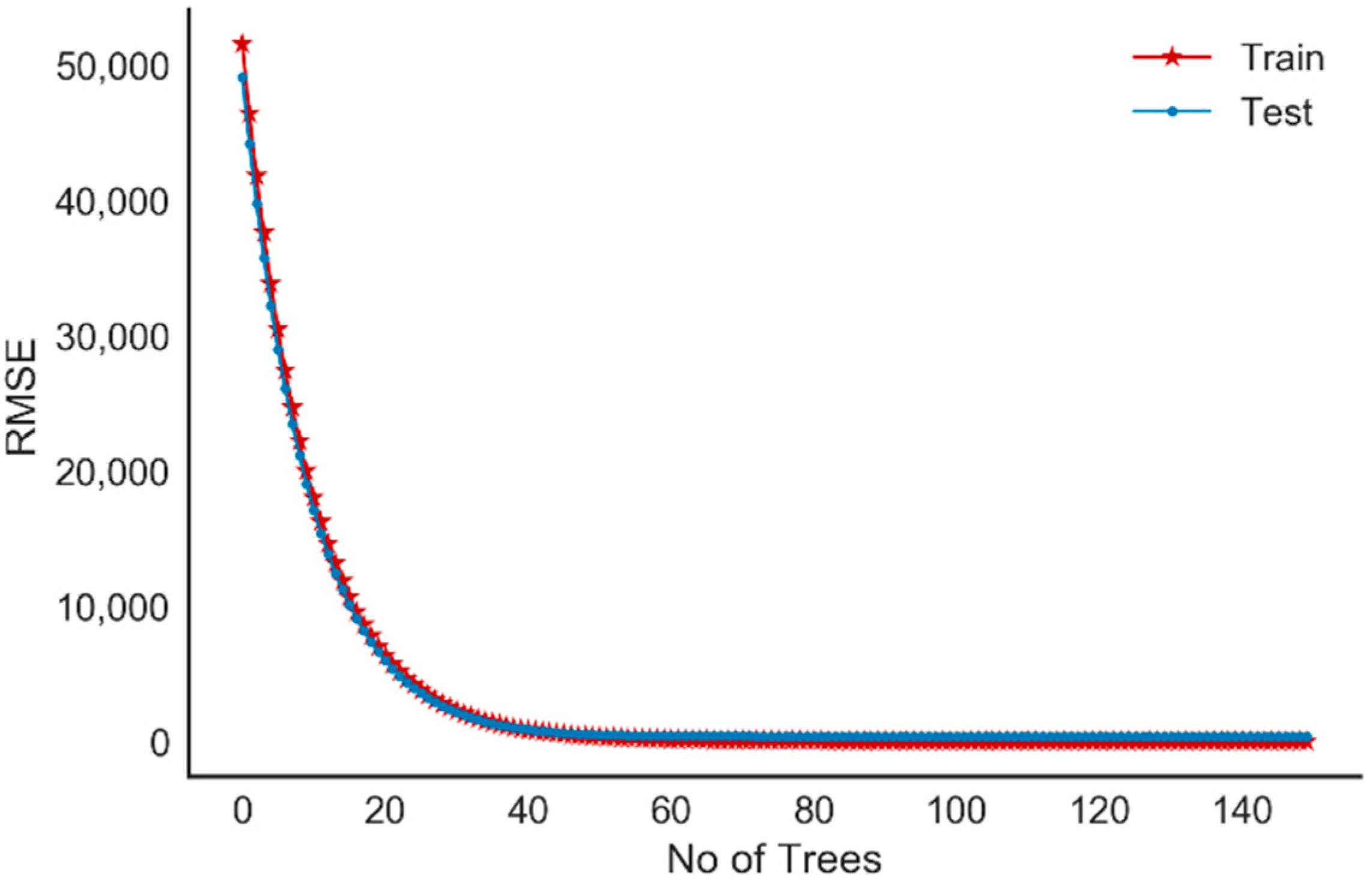
In order to prevent overfitting, we have implemented early stopping for the XGBoost model. The model is tested after every boosting round against test data. The training of the model finishes earlier if the evaluation metric does not improve for a given number of rounds. The learning curve illustrated in Figure 11 shows the validation and the training score of the fitted XGBoost model for varying numbers of trees. The mean squared errors for both the training and testing sets of XGBoost model decreases while adding sequential decision trees and converge at similar values, which indicates that the model does not suffer from either variance or bias error.
4.3. LSTM-RNN Model Training
After the machine learning benchmark selection, we build deep learning LSTM and GRU models as explained in our methodology. To model our current forecasting problem as a regression model, we state that the consumption at timestamp t + 1 (dependent variable) is a function of previous consumption at timestamps t, t − 1, t − 2, …, t − n. These time lags exhibit the conditional dependencies that will be useful for forecasting future values. Consequently, we construct many-to-one structure LSTMs and GRUs models as they are suitable deep learning models for sequential and temporal data.
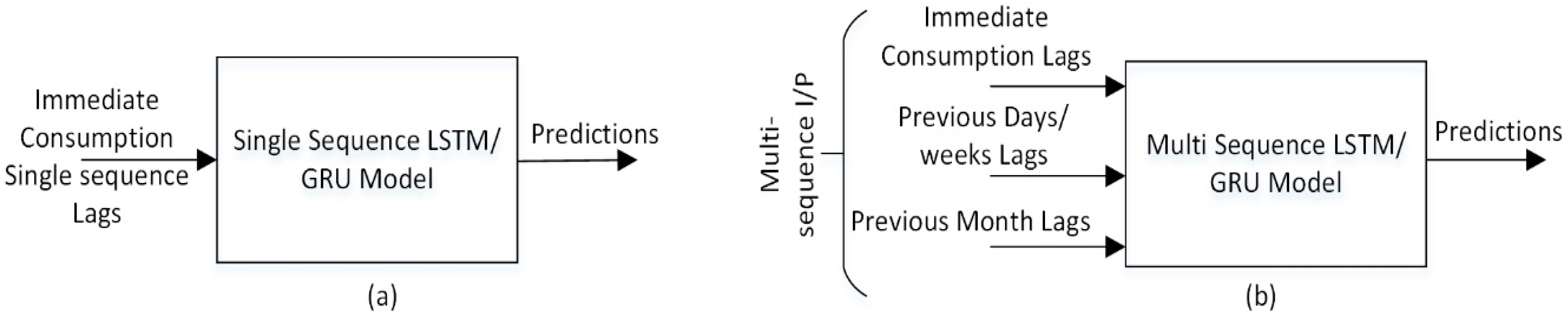
The larger the data, the greater is the scale of the LSTM network. In other terms, more hidden layers and neurons are used to model the future consumption while avoiding the overfitting problem. Otherwise, with less large neuron layers the model tends to underfit during the training. Actually, many parameters need to be carefully set to achieve high performance. They include the number of hidden layers, the number of neurons per layer, the number of epochs, the batch sizes, and the activation and optimization functions. The number of time lags that are used as inputs matches the size of the input layer of LSTM or GRU model, the neurons of the hidden layers are fully connected to other layers and the output layer has a single neuron. The mean squared error is used as loss function between the input and the corresponding neurons in the output layer. We use two different inputs configuration for LSTM and GRU models as shown in Figure 12a single sequence of immediate time lags and Figure 12b separated multi-sequence time lags other than immediate.
5. Experimental Results
In this section, we empirically determine deep learning model hyperparameters, examine both the ACF plot and autoregressive model, and then we derive several single and multi-sequence LSTM and GRU models using the electricity consumption dataset. When working with deep learning recurrent models, it is worth to use both the LSTM and GRU cells to recognize which one provides more accurate results for a particular network configuration and dataset. Obtaining good results using LSTM or GRU networks is not straightforward, as it requires consideration of the tuning of many hyperparameters. Table 2 lists the hyperparameters value sets to be tested for both LSTM and GRU models in our experimentation.
The network’s performance is highly dependent on the numbers of hidden layers and neurons per layer. For both the LSTM and GRU models, we obtained significantly better results when using three hidden layers with 100, 60 and 50 neurons, respectively. Increasing the number of layers beyond three did not, further reduced the loss. The number of epochs used were 150 neurons with batch size of 125 training examples. The LSTM and GRU models poorly perform on smaller window sizes of 5 and 10. The most effective length found was 30 time lags for the single sequence model. Empirical evaluations show that nonlinear activation function ReLU is found to be the best choice of the activation function for the hidden layers since is allows the best network performance. Unlike tanh and sigmoid activations, ReLU avoids vanishing gradient problem. Among the optimizers, ADAM, the adaptive moment estimation, performs faster convergence than SGD, the conventional stochastic gradient descent. With such an optimizer, there is no a need to specify and tune a learning rate as in the case of the stochastic gradient descent.
5.1. Models with Single-Sequence Input
After selecting the best network configuration and hyperparameters as explained previously, we train LSTM and GRU models using single input sequence of previous 30 lags. Table 3 shows the summary results, where both LSTM and GRU models achieve very close results and perform better than the benchmark.
5.2. Models with Multi-Sequence Input
After fitting LSTM model with a single input sequence of immediate 30 time lags, our second approach is to introduce separate past time sequences other than immediate. These time sequences are defined as days, weeks or months before. Therefore, we can consider the correlations between separated time sequences in order to further improve the model accuracy. In fact, exploring the relations between series of time lags sequences can provide the model with additional information that might be significant for accuracy improvement.
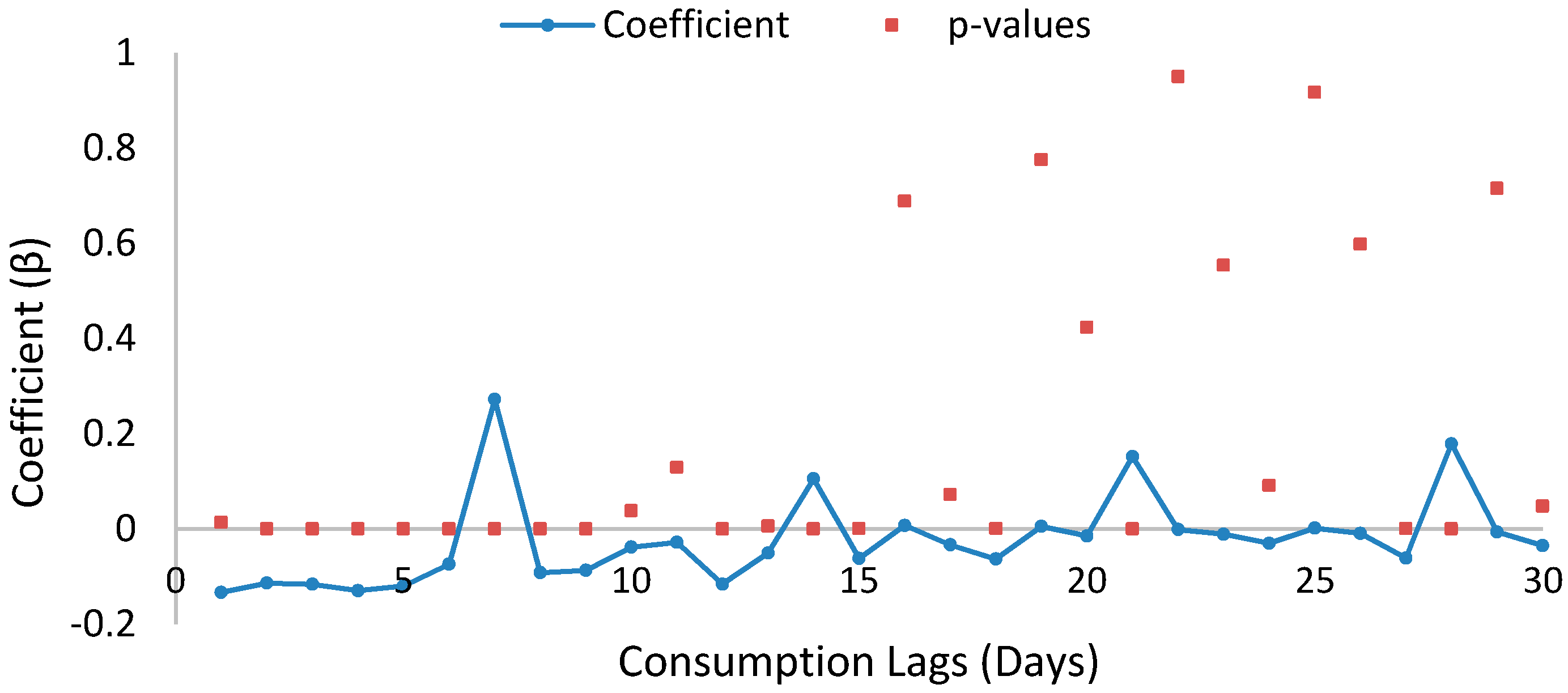
In order to have a broader understanding of which time lags are significant to be used for LSTM and GRU models, we developed an autoregressive model and autocorrelation function (ACF) plot. In autoregressive model, we assume that a variable depend on its previous values. An autoregressive model is developed to regress consumption using past lags up to 60 days, lag(x,1), lag(x,2) ……, lag(x,59), lag(x,60). The series is differential log to remove trends and stationarity. The plot of the lags coefficient for previous 60 days is shown in Figure 13 from which it is seen that lag coefficients 1, 2, 7, and 14 are important with small p-values; hence, the parameters are significant. The model has adjusted R-squared value of 0.775 and high F-statistic value of 375, suggesting that the parameter estimates for this model were all significant and non-zero.
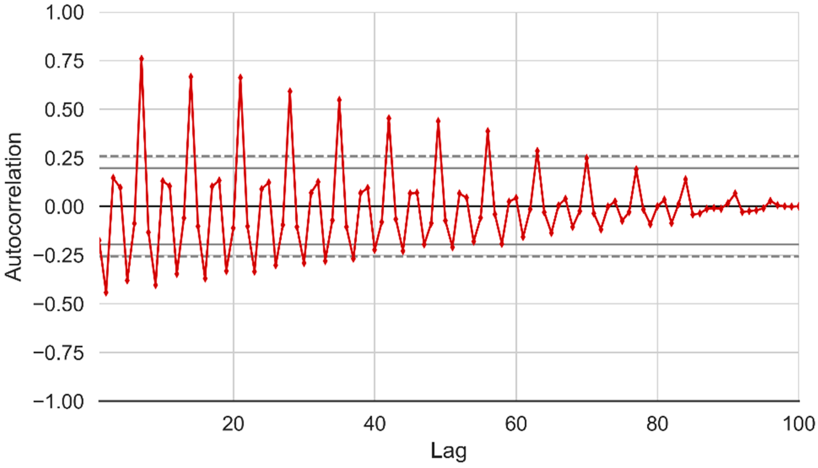
Furthermore, we analyze the ACF plot for the past 100 days’ time lags with 95% and 99% confidence intervals as indicated by the dotted lines in Figure 14. The values above the lines are statistically significant which reveals that lags up to past 60 days are significant
Based on the importance of lags, a series of experiments were performed using lag sequences of previous day, weeks and months as input to LSTM and GRU model. Obtained results are shown in Table 4.
By bringing additional past information using multiple timescale sequences, we further reduced forecasting errors compared to the single sequence LSTM and GRU models using only immediate lags. LSTM and GRU models at number ‘2’ and ‘6’ in the Table 4 with immediate, past day and past week lags have the lowest errors. Furthermore, these models allowed automatic identification of temporal relations using only time lag sequences as inputs without creating manual features, as made for machine learning models.
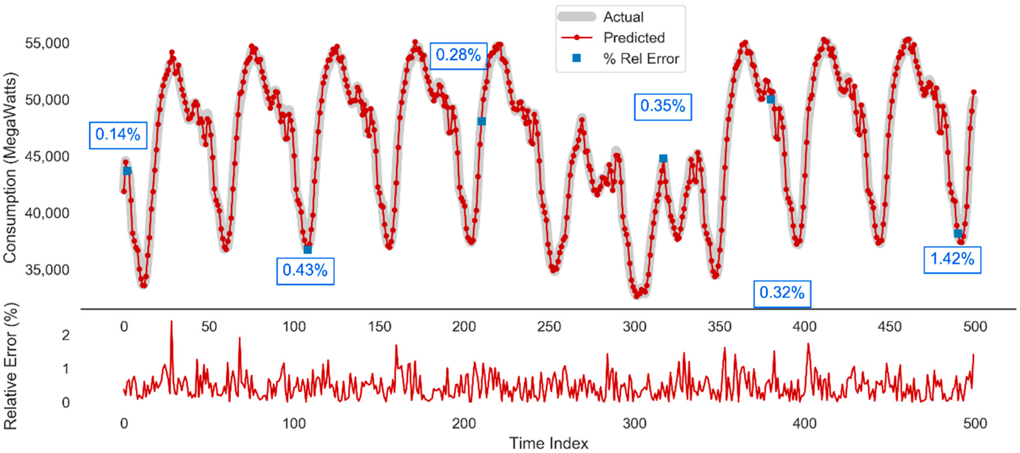
The plot of actual versus predicted forecast depicted in Figure 15 is capturing the achievement of the best performing multi-sequence LSTM model on two weeks of testing data. A good fit and stable prediction for the medium term horizon is obviously observed. Samples of relative errors values are captured and shown in different areas of the plot. Because of its small amplitude, we also track the variation of the relative error depicted down in Figure 15.
6. Models Validation
This section describes validation of single and multi-sequence deep learning LSTM and GRU models and discusses the threat of validity. The following three approaches are used for validation (a) time series split, (b) validation on short and medium term forecasting horizons and (c) walk forward sliding window approach.
6.1. Models Validation Using Time Series Split
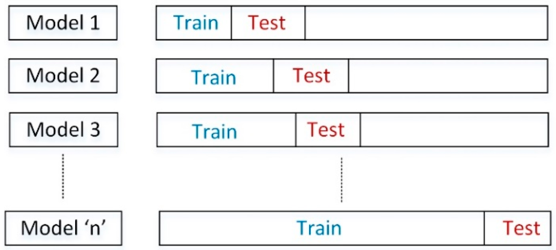
The chosen time series split is a variation of k-fold cross validation in which training sets are supersets of the training sets that come before them and the testing sets are chunks of data with higher indices than training set [34] as illustrated by Figure 16. Note that the test set size remains fixed while training set size will increase for every fold while retaining sequential order of data.
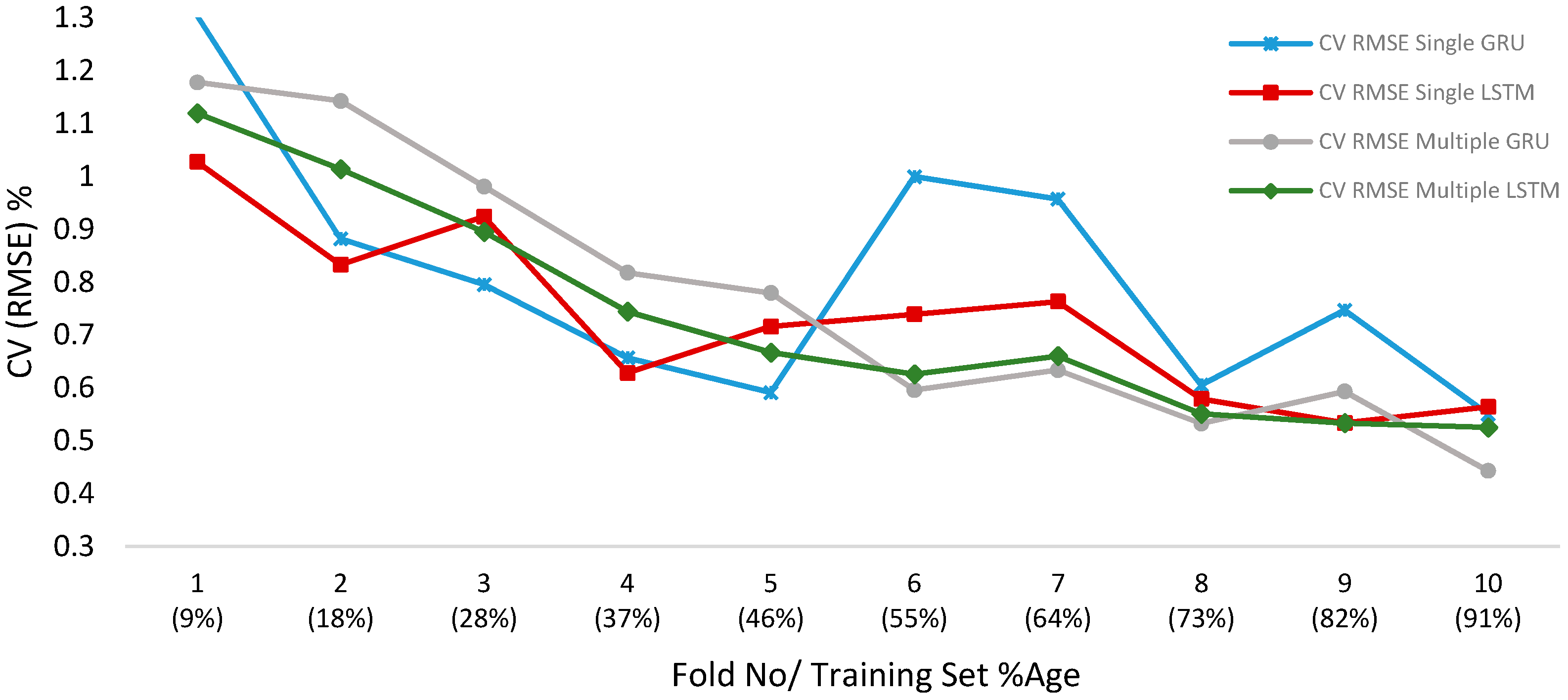
We use 10-fold time series validation to check performance of single and multi-sequence GRU and LSTM models. CV(RMSE) metrics for different models is plotted in Figure 17. The test set error is initially large on first few folds as we are using smaller training set size. The error decreases on the following folds. Furthermore, multiple sequence LSTM and GRU models errors are lower and relatively more stable than single sequence models as illustrated in Figure 17.
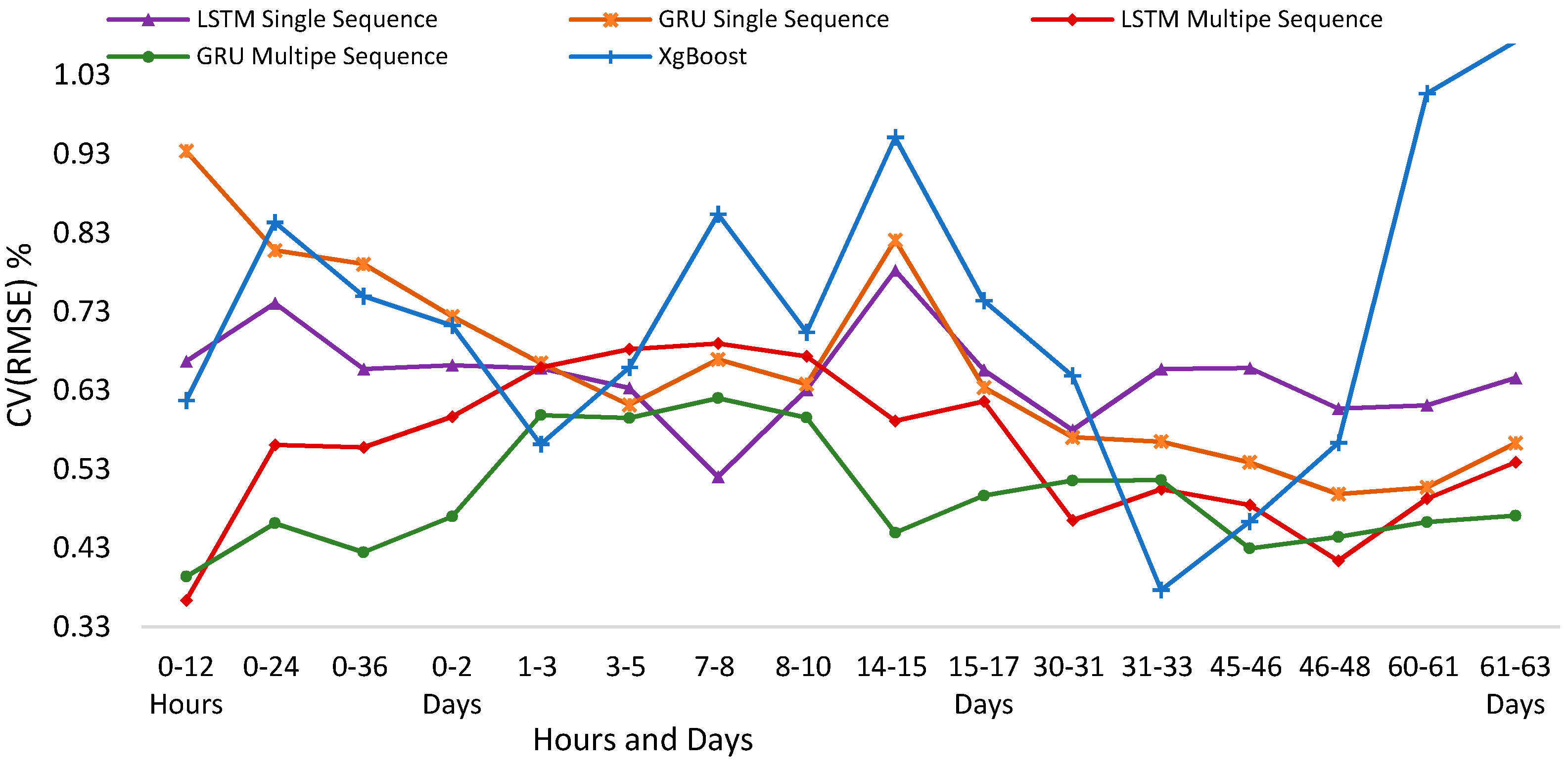
6.2. Validation on Short and Medium Term Forecasting Horizons
The aim of this section is to illustrate the time-variation in forecast accuracy of machine learning and deep learning models over short and medium term horizons. We plot the prediction performance of these models starting from the next few hours, days and up to two months into the future as shown in Figure 18. Looking at the results, we observe that the ensemble model has high variation in forecast errors on different forecasting horizons. Single sequence LSTM and GRU models also suffered from significant time variation in their performance compared to multi-sequence models. XGBoost model shows highest variation in CV(RMSE). With very comparable performances for both the short term and the medium term horizons, it is evident that multi-sequences models are more accurate and stable.
In order to establish that the variances of single and multi-sequence models, for different forecasting horizons, varies significantly, we perform two variances Levene’s and Bonett’s tests. These tests are inferential statistic tests used to assess the equality of variances and are valid for any continuous distribution. The statistical test will display the results for both methods. Null and alternate hypothesis are stated as follows:
Hypothesis 1 (H1).
Null Hypothesis, σ1/σ2 = K, i.e., The ratio between multi sequence GRU standard deviation (σ1) and single sequence GRU standard deviation (σ2) is equal to the hypothesized ratio K = 1.
Hypothesis 2 (H2).
Alternate Hypothesis, σ1/σ2 < K, i.e., The ratio between multi sequence GRU standard deviation (σ1) and single sequence GRU standard deviation (σ2) is less than the ratio K = 1.
From the test results, it is found that p-value for Bonetts test is 0.027, while for Levene test is 0.038. Thus, we conclude that the standard deviation of LSTM multiple sequence is significantly less than LSTM single sequence at 0.05 level of significance with a sample size of 16 as shown in Table 6.
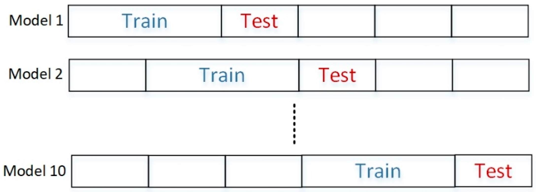
6.3. Validation Using Sliding Window Approach: t-Test for the Difference in Means
To validate the robustness of the multi-sequence LSTM model, we compare it to the single sequence model using a sliding window train test split as shown in Figure 19. Two sample t-test compares the means to determine whether single and multi-sequence models means are significantly different. The testing and training data sets sizes remains fixed for each window, while traversing the complete dataset.
The performance metrics are calculated for the ten models and the mean’s differences are compared using one tailed t-test assuming equal variances. The following hypothesis are tested:
Null Hypothesis, H1: μ1 − µ2 = 0,
Alternate Hypothesis, H2: μ1 < µ2.
Results obtained are shown in Table 7.
The p-value is 0.01569. Thus, we can conclude that that the mean of multi sequence LSTM is less than a single sequence at the 0.05 level of significance, with a sample size of ten.
6.4. Comparison with other Studies
Mean absolute percentage error is adopted here to assess the performance of our proposed forecasting model with existing short and medium term forecasting models as shown in Table 8. The half-hourly electricity consumption is predicted by the multi-sequence LSTM model for day, week, month and year horizons. The records of MAPE range between 0.48 and 0.55%. Comparing the MAPE of our model with the benchmarks in Table 8, shows that the proposed model has a good prediction accuracy.
Based on electrical forecasting studies [11,12,13,14,18,19,20,21,22,23,24,25,26,35,36], researchers have used three broad categories of input features for load forecasting namely; historical lags, meteorological and calendar related features. The type of features used by various researchers depends on the forecasting horizon (short or medium term), temporal resolution, spatial characteristics and underlying data characteristics in addition of the data availability and the ways of its collection.
Compared to other models the multi-sequence LSTM using only past load lags as input features exhibits superior capability as it is able to learn complex time series patterns with long temporal dependency characteristics. Furthermore, the proposed model uses only the past load lags as inputs. It in fact exploits implicit information contained in these lags, which reduces the burden of collecting meteorological or other categories of data for modeling purposes. However, LSTM based modeling necessitates careful hyperparameter tuning to avoid overfitting and requires longer training times than machine learning models.
6.5. Threat to Validity
The threats to construct validity of our study are related to two issues. The first one is the adequacy of data features used as predictors of energy consumption. This issue has been considered early in our project, where various features like weather information has been added as input, and then unselected by several techniques of features selection. The second threat concerns the algorithms used in our data-mining framework that could be on-the-shelf using assumptions that are incompatible with energy forecasting context. To alleviate this threat, we developed, tested and tuned all the algorithms in-house.
The internal validity of our results concerns three threats. The first is the extent to which the size of training data is suitable to the multi-sequence LSTM model training that requires a long history of data recording. It should reflect the complex electric load characteristics exhibited by time series, like periodicity, data frequency, trends, levels, structural breaks and calendar effects. In particular, the complex daily, weekly, monthly and yearly patterns of electric load. To alleviate such a threat, we used the power consumption data RTE covering a consumption period of 9 years (i.e., from January 2008 to December 2017). The second threat is the overfitting of the derive forecasting. In general, an excessive training in the case of complex prediction models leads to a bad generalization. To prevent our LSTM overfitting, we have proceeded to randomly modify the training examples for each epoch. Such a training strategy helps to improve the ability of the model to consider various circumstances and thus enhance its generalization. In addition, intelligent stopping criteria of the training process are used to reduce overfitting such as early stopping when the minimum error is achieved on the test set. The third threat is associated with the selection of machine-learning benchmarks. They may miss-represent the state of the art of the techniques used in the energy prediction. Accordingly, we have compared our approach to the most successful machine learning as reported in the recent literature and including our latest proposed single sequence LSTM forecasting model.
The threat to the external validity is related to the performance of our multi-sequence LSTM when it is used in new circumstances of energy consumption. This is alleviated by carefully considering the electric load domain characteristics. Indeed, the rationale behind using multiple sequence of inputs is to introduce generic domain knowledge such as periodicity, data frequency, trends, levels, structural breaks and calendar effects. In addition, this threat is initially alleviated by deep learning approach capability to capture generalizable patterns. Furthermore, three different validation approaches are used to evaluate the performance of the proposed multi-sequence LSTM on unseen data, namely, time series split, validation on short and medium term forecasting horizons and walk forward sliding window. Details on the application of these approaches can be seen in Section 6.3.
7. Conclusions
The rigorous management of sustainable energy systems is very dependent on the accuracy of forecasting models. Electricity consumption behavior is inherently transient in nature, shaped by medium and long term dependencies. In this research work, we have used single and multi-sequence LSTM and GRU models to model these data dependencies in time series. The multi-sequence model enabled capturing the information in electric consumption time series and exploiting the information contained in different timescales. For comparison purposes, we implemented ANN and ensemble based approaches, and the best performing amongst them was used as our benchmark model.
We demonstrated that by using multiple timescale sequences as inputs for both LSTM and GRU models, we were able to learn accurately crucial information over longer history timeframes. GRU and LSTM models using immediate, one day and one week before lag inputs gave the most accurate and stable results. They allow the automation of temporal relations identification using only time lags features data at the cost of larger sets of parameters to be tuned. In addition, output from multi-sequence models were found to be more robust against time variations then machine leaning and single-sequence models. Precisely, with multi-sequence LSTM and GRU, we have reduced the prediction error by more than 15% and 21%, respectively (i.e., RMSE drops from 346.34 to 293.74 MW with LSTM and from 339.22 to 266.57 MW with GRU). Thus, we conclude that exploring the relations between multi-sequence time scales can provided the model with additional information which has significantly improved the model training and accuracy while providing predictions that were robust against time variations.
As future works, we will explore various met-heuristics approaches to find the appropriate settings of the above-proposed multi-sequence LSTM and GRU models. Such approach will avoid try-and-see based configurations that are not optimal and time consuming especially in the case of deep learning.
Author Contributions
This paper the fruit of all authors’ collaboration. Problem formulation and Conceptualization S.B. and A.F.; Methodology, S.B., A.F. and A.O.; Software, A.F. and S.B.; Validation, S.B., A.F. and A.O.; Writing-Original Draft Preparation, S.B., A.F., M.A.S. and A.O.; Writing-Review & Editing, S.B., A.F., A.O. and M.A.S.; Supervision and Project Administration, S.B.; Funding Acquisition, S.B. and M.A.S.
Funding
This work was supported by a UPAR grant from the United Arab Emirates University, under grant G00001930.
Conflicts of Interest
The authors declare no conflict of interest.
Nomenclature
| ACF | autocorrelation function |
| ANN | artificial neural network |
| AR | Autoregressive |
| ARIMA | autoregressive integrated moving average |
| CV | coefficient of variation |
| DNN | deep neural networks |
| GRU | gated recurrent unit |
| LSTM | Long short term memory |
| MAE | mean absolute error |
| MAPE | Mean absolute percentage error |
| MLP | multi-layer perceptron |
| RNN | Recurrent neural networks |
| RMSE | root mean squared error |
| STLF | short-term load forecasting |
| SVM | support vector machines |
References
- Stoft, S. Power system economics. J. Energy Lit. 2002, 8, 94–99. [Google Scholar]
- Zhang, G.P. Time series forecasting using a hybrid ARIMA and neural network model. Neurocomputing 2003, 50, 159–175. [Google Scholar] [CrossRef]
- Box, G.E.; Jenkins, G.M.; Reinsel, G.C. Time Series Analysis: Forecasting and Control; John Wiley & Sons: Hoboken, NJ, USA, 2011; Volume 734. [Google Scholar]
- Hernandez, L.; Baladron, C.; Aguiar, J.M.; Carro, B.; Sanchez-Esguevillas, A.J.; Lloret, J.; Massana, J. A survey on electric power demand forecasting: Future trends in smart grids, microgrids and smart buildings. IEEE Commun. Surv. Tutor. 2014, 16, 1460–1495. [Google Scholar] [CrossRef]
- Graves, A.; Jaitly, N. Towards end-to-end speech recognition with recurrent neural networks. In Proceedings of the International Conference on Machine Learning, Beijing, China, 21–26 June 2014; pp. 1764–1772. [Google Scholar]
- Mao, J.; Xu, W.; Yang, Y.; Wang, J.; Huang, Z.; Yuille, A. Deep captioning with multimodal recurrent neural networks (m-rnn). arXiv, 2014; arXiv:1412.6632. [Google Scholar]
- Sutskever, I.; Vinyals, O.; Le, Q.V. Sequence to sequence learning with neural networks. In Proceedings of the Neural Information Processing Systems 2014, Montréal, QC, Canada, 8–13 December 2014; pp. 3104–3112. [Google Scholar]
- Hochreiter, S.; Schmidhuber, J. LSTM can solve hard long time lag problems. In Proceedings of the Neural Information Processing Systems 1997, Denver, CO, USA, 5 May 1997; pp. 473–479. [Google Scholar]
- Cho, K.; Van Merriënboer, B.; Gulcehre, C.; Bahdanau, D.; Bougares, F.; Schwenk, H.; Bengio, Y. Learning phrase representations using RNN encoder-decoder for statistical machine translation. arXiv, 2014; arXiv:1406.1078. [Google Scholar]
- Bouktif, S.; Fiaz, A.; Ouni, A.; Serhani, M. Optimal deep learning LSTM model for electric load forecasting using feature selection and genetic algorithm: Comparison with machine learning approaches. Energies 2018, 11, 1636. [Google Scholar] [CrossRef]
- Wang, Z.; Srinivasan, R.S. A review of artificial intelligence based building energy use prediction: Contrasting the capabilities of single and ensemble prediction models. Renew. Sustain. Energy Rev. 2017, 75, 796–808. [Google Scholar] [CrossRef]
- Liu, N.; Tang, Q.; Zhang, J.; Fan, W.; Liu, J. A hybrid forecasting model with parameter optimization for short-term load forecasting of micro-grids. Appl. Energy 2014, 129, 336–345. [Google Scholar] [CrossRef]
- Ryu, S.; Noh, J.; Kim, H. Deep neural network based demand side short term load forecasting. Energies 2016, 10, 3. [Google Scholar] [CrossRef]
- Hagan, M.T.; Behr, S.M. The time series approach to short term load forecasting. IEEE Trans. Power Syst. 1987, 2, 785–791. [Google Scholar] [CrossRef]
- Taylor, J.W. Short-term electricity demand forecasting using double seasonal exponential smoothing. J. Oper. Res. Soc. 2003, 54, 799–805. [Google Scholar] [CrossRef] [Green Version]
- Taylor, J.W.; De Menezes, L.M.; McSharry, P.E. A comparison of univariate methods for forecasting electricity demand up to a day ahead. Int. J. Forecast. 2006, 22, 1–16. [Google Scholar] [CrossRef] [Green Version]
- Park, D.C.; El-Sharkawi, M.A.; Marks, R.J.; Atlas, L.E.; Damborg, M.J. Electric load forecasting using an artificial neural network. IEEE Trans. Power Syst. 1991, 6, 442–449. [Google Scholar] [CrossRef] [Green Version]
- Hernandez, L.; Baladrón, C.; Aguiar, J.M.; Carro, B.; Sanchez-Esguevillas, A.J.; Lloret, J. Short-term load forecasting for microgrids based on artificial neural networks. Energies 2013, 6, 1385–1408. [Google Scholar] [CrossRef]
- Hippert, H.S.; Pedreira, C.E.; Souza, R.C. Neural networks for short-term load forecasting: A review and evaluation. IEEE Trans. Power Syst. 2001, 16, 44–55. [Google Scholar] [CrossRef]
- Yukseltan, E.; Yucekaya, A.; Bilge, A.H. Forecasting electricity demand for Turkey: Modeling periodic variations and demand segregation. Appl. Energy 2017, 193, 287–296. [Google Scholar] [CrossRef]
- Zhang, F.; Deb, C.; Lee, S.E.; Yang, J.; Shah, K.W. Time series forecasting for building energy consumption using weighted Support Vector Regression with differential evolution optimization technique. Energy Build. 2016, 126, 94–103. [Google Scholar] [CrossRef]
- Papadopoulos, S.; Karakatsanis, I. Short-term electricity load forecasting using time series and ensemble learning methods. In Proceedings of the IEEE Power and Energy Conference at Illinois (PECI), Champaign, IL, USA, 20–21 February 2015; pp. 1–6. [Google Scholar]
- Dudek, G. Short-term load forecasting using random forests. In Intelligent Systems’ 2014; Springer: Cham, Switzerland, 2015; pp. 821–828. [Google Scholar]
- Wang, W.; Shi, Y.; Lyu, G.; Deng, W. Electricity Consumption Prediction Using XGBoost Based on Discrete Wavelet Transform. DEStech Trans. Comput. Sci. Eng. 2017. [Google Scholar] [CrossRef] [Green Version]
- Hossen, T.; Plathottam, S.J.; Angamuthu, R.K.; Ranganathan, P.; Salehfar, H. Short-term load forecasting using deep neural networks (DNN). In Proceedings of the 2017 North American IEEE Power Symposium (NAPS), Morgantown, WV, USA, 17–19 September 2017; pp. 1–6. [Google Scholar]
- He, W. Load forecasting via deep neural networks. Procedia Comput. Sci. 2017, 122, 308–314. [Google Scholar] [CrossRef]
- Zheng, H.; Yuan, J.; Chen, L. Short-Term Load Forecasting Using EMD-LSTM Neural Networks with a Xgboost Algorithm for Feature Importance Evaluation. Energies 2017, 10, 1168. [Google Scholar] [CrossRef]
- Colah.github.io. Understanding LSTM Networks—Colah’s Blog. Available online: http://colah.github.io/posts/2015-08-Understanding-LSTMs (accessed on 24 August 2018).
- Patterson, J.; Gibson, A. Deep Learning: A Practitioner’s Approach; O’Reilly Media, Inc.: Sevvan, CA, USA, 2017. [Google Scholar]
- Chung, J.; Gulcehre, C.; Cho, K.; Bengio, Y. Empirical evaluation of gated recurrent neural networks on sequence modeling. arXiv, 2014; arXiv:1412.3555. [Google Scholar]
- Wei, Y.; Zhang, X.; Shi, Y.; Xia, L.; Pan, S.; Wu, J.; Zhao, X. A review of data-driven approaches for prediction and classification of building energy consumption. Renew. Sustain. Energy Rev. 2018, 82, 1027–1047. [Google Scholar] [CrossRef]
- Yildiz, B.; Bilbao, J.I.; Sproul, A.B. A review and analysis of regression and machine learning models on commercial building electricity load forecasting. Renew. Sustain. Energy Rev. 2017, 73, 1104–1122. [Google Scholar] [CrossRef]
- RTE France. Bilans Électriques Nationaux. Available online: http://www.rte-france.com/fr/article/bilans-electriques-nationaux (accessed on 7 February 2018).
- sklearn.model_selection.TimeSeriesSplit—scikit-learn 0.20.1 Documentation. 2018. Available online: https://scikit-learn.org/stable/modules/generated/sklearn.model_selection.TimeSeriesSplit.html (accessed on 20 March 2018).
- Massana, J.; Pous, C.; Burgas, L.; Melendez, J.; Colomer, J. Short-term load forecasting in a non-residential building contrasting models and attributes. Energy Build. 2015, 92, 322–330. [Google Scholar] [CrossRef] [Green Version]
- Wang, Z.; Wang, Y.; Srinivasan, R.S. A novel ensemble learning approach to support building energy use prediction. Energy Build. 2018, 159, 109–122. [Google Scholar] [CrossRef]
Figure 1.
Unfolding in time of the computation of RNN network.

Figure 2.
Information flow in an LSTM block of the RNN.

Figure 3.
Information flow in GRU block of the RNN.

Figure 4.
Proposed forecasting methodology.

Figure 5.
Electricity load versus time: daily, weekly and monthly patterns. (a) Half hourly consumption; (b) Weekly Consumption; (c) Monthly Consumption.
Figure 5.
Electricity load versus time: daily, weekly and monthly patterns. (a) Half hourly consumption; (b) Weekly Consumption; (c) Monthly Consumption.

Figure 6.
(a) Box plot of load consumption for high and low temperatures; (b) Factor plot of electric load consumption weekend vs. weekday.
Figure 6.
(a) Box plot of load consumption for high and low temperatures; (b) Factor plot of electric load consumption weekend vs. weekday.

Figure 7.
Correlation with previous 6 load lags.

Figure 8.
Joint plot of electric load vs. (a) temperature (b) humidity (c) wind speed.

Figure 9.
Benchmark selection using ANN and Ensemble models.

Figure 10.
Predicted versus actual load by XGBoost model.

Figure 11.
Learning curve for the XGBoost regressor.

Figure 12.
Inputs to LSTM and GRU models (a) Single Input sequence (b) Multiple Input sequence.

Figure 13.
Coefficients of the autoregressive model.

Figure 14.
Autocorrelation function (ACF) plot.

Figure 15.
Actual vs. predicted forecast achieved by the multi-sequence LSTM model and relative error variation.
Figure 15.
Actual vs. predicted forecast achieved by the multi-sequence LSTM model and relative error variation.

Figure 16.
Time Series Split for Model Validation.

Figure 17.
Time series cross validation with multiple Train-Test Splits.

Figure 18.
Forecasting Horizon for Machine Learning and Deep Learning Models.

Figure 19.
Sliding window train-test split for comparison of means.


Table 1.
Performance Metrics of ANN and Ensemble Models.
| Model | RMSE | CV (RMSE) | MAE |
|---|---|---|---|
| ANN | 725.89 | 1.311 | 559.63 |
| Random Forest | 527.25 | 0.952 | 368.91 |
| Extra Trees Regressor | 492.13 | 0.889 | 346.44 |
| Gradient Boosting | 455.84 | 0.823 | 320.72 |
| Extreme Gradient Boosting | 440.16 | 0.795 | 311.43 |
Table 2.
Hyperparameters testing for experiment.
| No | Hyperparameter | Option |
|---|---|---|
| 1 | Time Lags | 10, 20, 30, 40 |
| 2 | No of Hidden Layers | 1, 2, 3, 4 |
| 3 | No of Neurons in Hidden layer | 30, 40, 50, 60 |
| 4 | Batch Size | 50 to 200 |
| 5 | Epochs | 50 to 150 |
| 6 | Activation Function | Sigmoid, hyperbolic tangent (tanh) and rectified linear unit (ReLU) |
| 7 | Optimizers. | ADAM (adaptive moment estimation), SGD (Stochastic gradient descent), RMSProp (Root Mean Square Propagation) |
Table 3.
Performance Metrics Comparison of single sequence models.
| Metrics | LSTM Model 30 Lags | GRU Model 30 Lags | XGBoost Model Metrics |
|---|---|---|---|
| RMSE | 346.34 | 339.22 | 440.16 |
| CV(RMSE) | 0.622 | 0.611 | 0.795 |
| MAE | 257.05 | 251.66 | 311.43 |
Table 4.
Impact of the Different timescales on LSTM and GRU models performance.
| No | Model Inputs | Errors LSTM | Errors GRU | ||||
|---|---|---|---|---|---|---|---|
| Input 1 | Input 2 | Input 3 | MAE | RMSE | MAE | RMSE | |
| 1 | Immediate 10 | 2 days, 10 lags | 3 days, 10 lags | 315.41 | 394.70 | 352.34 | 270.56 |
| 2 | Immediate 10 | 1 day, 10 lags | 1 week, 10 lags | 220.79 | 293.74 | 233.18 | 312.64 |
| 3 | Immediate 10 | 1 week, 10 lags | 2 week 10 lags | 293.02 | 388.35 | 234.62 | 326.48 |
| 4 | Immediate 10 | 1 week, 10 lags | 1 Month, 10 lags | 252.05 | 351.15 | 324.67 | 434.19 |
| 5 | Immediate 10 | 1 month,10 lags | 2 Month, 10 lags | 389.45 | 512.40 | 380.26 | 490.10 |
| 6 | Immediate 20 | 1 day, 20 lags | 1 week, 20 Lags | 251.16 | 327.48 | 202.15 | 266.57 |
| 7 | Immediate 20 | 1 day, 20 lags | 2 week, 20 Lags | 239.58 | 314.53 | 242.14 | 317.08 |
| 8 | Immediate 20 | 1 week, 20 lags | 2 week, 20 Lags | 291.51 | 386.30 | 251.84 | 353.36 |
| 9 | Immediate 20 | 1 week, 20 lags | 1 month,20 Lags | 332.86 | 417.32 | 234.87 | 334.80 |
| 10 | Immediate 20 | 1 month 20 lags | 2 Month, 20 lags | 323.88 | 428.79 | 473.01 | 585.77 |
Table 5.
Performance Metrics for single and multiple-sequence models using time series split.
| Metric/Model | Single Sequence | Multiple Sequence | |||
|---|---|---|---|---|---|
| LSTM | GRU | LSTM | GRU | ||
| MAE | Mean | 294.81 | 342.28 | 307.12 | 329.27 |
| Std. Deviation | 66.84 | 103.96 | 87.61 | 110.61 | |
| RMSE | Mean | 403.47 | 446.62 | 404.94 | 425 |
| Std. Deviation | 89.65 | 129.03 | 115.18 | 142.02 | |
Table 6.
Statistics for single and multiple-sequence models on various forecasting horizons.
| Model | Standard Deviation CV(RMSE) % | Variance | 95% Upper Bound for σ |
|---|---|---|---|
| Single-sequence LSTM | 0.126 | 0.016 | 0.186 |
| Multiple-sequence LSTM | 0.071 | 0.005 | 0.099 |
Table 7.
t-Test for the difference in means: Sliding window approach.
| Model | Mean CV (RMSE) (%) | Variance |
|---|---|---|
| Single Sequence LSTM | 0.64231 | 0.004023 |
| Multiple Sequence LSTM | 0.58994 | 0.001603 |
Table 8.
Reviewed Papers for features and MAPE.
| Ref. | MAPE (%) | Horizon | Features | Approach |
|---|---|---|---|---|
| [20] | 1.34–3.59 | Annual Predictions | Harmonics of sinusoidal variations | Linear regression |
| [22] | 1.32–2.62 | Day ahead | Past loads, Std dev, calendar features (month, day, hour) | SARIMA, SARIMAX, random forests gradient boosting regression trees |
| [23] | 0.92–2.64 | Day ahead | Past loads | Random forest |
| [25] | 1.19–3.29 | 90 days | Weather and load data | Deep neural network |
| [35] | 0.06–4.68 | 90 days | Electrical load, weather, indoor and calendar data. | MLR, MLP, SVR |
| [36] | 2.97–4.62 | 2 weeks ahead | Meteorological, occupancy, calendar | Ensemble bagging trees |
| [Present work] | 0.48–0.55 | Day, weak, month, year | Multi-sequence past loads | LSTM |
© 2019 by the authors. Licensee MDPI, Basel, Switzerland. This article is an open access article distributed under the terms and conditions of the Creative Commons Attribution (CC BY) license (http://creativecommons.org/licenses/by/4.0/).
Share and Cite
MDPI and ACS Style
Bouktif, S.; Fiaz, A.; Ouni, A.; Serhani, M.A. Single and Multi-Sequence Deep Learning Models for Short and Medium Term Electric Load Forecasting. Energies 2019, 12, 149. https://doi.org/10.3390/en12010149
AMA Style
Bouktif S, Fiaz A, Ouni A, Serhani MA. Single and Multi-Sequence Deep Learning Models for Short and Medium Term Electric Load Forecasting. Energies. 2019; 12(1):149. https://doi.org/10.3390/en12010149
Chicago/Turabian StyleBouktif, Salah, Ali Fiaz, Ali Ouni, and Mohamed Adel Serhani. 2019. "Single and Multi-Sequence Deep Learning Models for Short and Medium Term Electric Load Forecasting" Energies 12, no. 1: 149. https://doi.org/10.3390/en12010149
Note that from the first issue of 2016, this journal uses article numbers instead of page numbers. See further details here.