Realistic Wind Farm Layout Optimization through Genetic Algorithms Using a Gaussian Wake Model


Wind Engineering and Renewable Energy Laboratory (WiRE), École Polytechnique Fédérale de Lausanne (EPFL), CH-1015 Lausanne, Switzerland
*
Author to whom correspondence should be addressed.
Energies 2018, 11(12), 3268; https://doi.org/10.3390/en11123268
Submission received: 2 October 2018
/
Revised: 29 October 2018
/
Accepted: 14 November 2018
/
Published: 23 November 2018
Abstract
:Wind Farm Layout Optimization (WFLO) can be useful to minimize power losses associated with turbine wakes in wind farms. This work presents a new evolutionary WFLO methodology integrated with a recently developed and successfully validated Gaussian wake model (Bastankhah and Porté-Agel model). Two different parametrizations of the evolutionary methodology are implemented, depending on if a baseline layout is considered or not. The proposed scheme is applied to two real wind farms, Horns Rev I (Denmark) and Princess Amalia (the Netherlands), and two different turbine models, V80-2MW and NREL-5MW. For comparison purposes, these four study cases are also optimized under the traditionally used top-hat wake model (Jensen model). A systematic overestimation of the wake losses by the Jensen model is confirmed herein. This allows it to attain bigger power output increases with respect to the baseline layouts (between 0.72% and 1.91%) compared to the solutions attained through the more realistic Gaussian model (0.24–0.95%). The proposed methodology is shown to outperform other recently developed layout optimization methods. Moreover, the electricity cable length needed to interconnect the turbines decreases up to 28.6% compared to the baseline layouts.
1. Introduction
Different economic reasons, mainly related to the need to best harness areas with a high wind resource while restraining the cost of electricity cable, make wind turbines be installed in clusters, widely known as wind farms. However, at the same time, this necessity to restrain the area where the devices are settled gives rise to unwanted flow disruptions, mainly produced by turbine wakes affecting downstream turbines. This issue can result in a remarkable reduction of the overall wind power output in the wind farm for some wind directions (e.g., [1,2,3]). In the last decade, it has been shown that the optimization of the turbine layout in a wind farm can be used to minimize the wake effects and, therefore, maximize the overall wind power production of the facility (e.g., [4,5,6]).
The high variability of the boundary layer flow climatology in a wind farm requires that each possible layout solution is assessed under multiple wind conditions (direction, magnitude) in order to obtain a realistic approach of its wind power capability [3,7,8]. Considering this framework for wind farm layout optimization is far from being computationally feasible through the numerical models capable of representing the wake interactions (e.g., Large Eddy Simulation, LES). This is usually overcome through the implementation of simple and computationally inexpensive analytical wake models, where the flow conditions are solved through simple analytic expressions and only over specific points of interest inside a wind farm. Different analytical turbine wake modelling approaches have been developed during the last few decades. Jensen [9] (further developed in Katic et al. [10]) designed a mass-conservation model with a top-hat velocity deficit profile for the wake flow behind a wind turbine. Due to its simplicity and easy applicability, it became the reference model used in the last few decades. Further improvements have been attained in recent years. Always under a top-hat scheme, Frandsen and Thøgersen [11] introduced momentum conservation in the parametrization of the wake. Jiménez et al. [12] developed a model for the deflection of a wake, when the turbine is controlled with yaw. This was used later on by Gebraad et al. [5] in combination with the Jensen [9] model. Finally, Bastankhah and Porté-Agel [13] derived an analytical model based on mass and momentum conservation, together with the assumption of a more realistic, self-similar Gaussian shape of the velocity deficit. The authors provided validations of the model against high resolution wind-tunnel measurements and LES data, showing a clear improvement of the representation of the wake compared to previous approaches [9,14], thus making it especially suitable for wind farm layout optimization problems.
Wind Farm Layout Optimization (WFLO) has been addressed by numerous works, which implemented different optimization methods (see the review by Herbert-Acero et al. [15] and references therein). Several of them have used gradient-based WFLO solvers, such as Combinatorial optimization [16], Sequential Linear (SLP) or Quadratic (SQP) Programming [6,17,18,19] or RANS-based gradients [20]. Most contributions, however, have used gradient-free methods, most of them in the field of Soft Computing [21] (SC). SC entails a subset of Artificial Intelligence [22] consisting of different non-deterministic, heuristic and metaheuristic techniques which are characterized by exploiting the tolerance for uncertainty to yield efficient optimization solutions at the same time with a very low computational cost compared to numerical simulations, without dismissing beforehand any possible solution to the problem. To date, most contributions on WFLO have implemented different sub-categories of SC, including Greedy [23,24] Monte Carlo [25], Pattern Search [26], or Local Search [27] heuristics, or Simulated Annealing [28,29] or Evolutionary Computation (EC) metaheuristics such as Particle Swarm Optimization [4,30,31], Ant Colony [32] or Genetic Algorithms (e.g., Bilbao and Alba [29], Salcedo-Sanz et al. [33,34], Huang [35], Liu and Wang [36], Gao et al. [37], Réthoré et al. [38]). In an EC optimization tool, different principles based on biological evolution are used, while keeping diversity by considering a big enough set of potential solutions (population). EC has proven to be highly effective in many diverse optimization problems [39], including studies on wind, as wind shear control within the aero-space industry [40] or wind variability estimation [41,42,43].
EC has been proven an efficient resource in WFLO. A simple Genetic Algorithm (GA) proposed by Mosetti et al. [44] was the first to show the advantages of EC tools in the field, and became a benchmark for multiple subsequent works. Since then, other contributions have used more complex EC versions while addressing multiple WFLO aspects. Grady et al. [45] considered different wind speeds and angles, and Emami and Noghreh [46] provided additional economic constraints to the cost function. In turn, Elkinton et al. [47] implemented a genetic algorithm where several variables as sea floor properties or distance to the coast were also considered. González et al. [48] introduced an algorithm that included some restricted turbine locations, while Ituarte-Villarreal and Espiritu [49] proposed Viral System Algorithms [50] to address WFLO. More recently Parada et al. [51] applied an up-to-date GA [52] to the Mosetti et al. [44] problem. However, all WFLO contributions mentioned consider at least either a gridded, limited matrix of coordinates for the turbine positions (usually squared grids [16,17,23,24,25,29,30,31,35,36,44,45,46,48,49,51], or either a highly idealized wind climatology [4,6,18,19,20,26,27,28,32,33,34,37,38,47]. Regarding this last point, it has been shown that the estimate of the overall wind power output in a wind farm does not become reliable until the used wind rose attains resolutions of approximately 3° and 1 m/s [53], and “using few sectors (12 as in the common practice) will lead to impressively high but unreal improvement on power” [54].
In latest years, some WFLO works have started considering more realistic conditions, as a continuous space for the turbine positioning and higher resolutions in the wind variability. Regarding this, Feng and Shen [53,55] implemented a Random Search (RS) routine in a real wind farm (Horns Rev I [56]) using a high resolution, Weibull-fitted wind climatology. Then, Feng et al. [54] further developed the RS-based procedure to address multi-objective WFLO experiments in the same farm. More recently, Gebraad et al. [57] implemented SQP in Princess Amalia Wind Farm [58] by considering a high resolution wind rose. A common feature of these WFLO contributions is that they all use the analytical wake model proposed by Jensen [9], which has been recently shown to considerably overestimate the wake effects in a wind farm [8] compared to the Gaussian model from Bastankhah and Porté-Agel [13] (hereafter, BPA14). This, added to the fact that resources as genetic algorithms have only been implemented on WFLO under simplified assumptions through rather standard versions, provides an excellent opportunity to investigate WFLO through further innovative and WFLO-specific EC solutions in a more realistic and efficient framework. This work develops this idea by designing, implementing and validating different novel EC-based WFLO strategies upon the Gaussian wake model from BPA14 and, for comparison, over a traditionally used wake model as the Jensen [9] model. In addition, herein we aim at assessing the sensitivity of the developed tools to different variables, such as the local climatology, the wind farm geometry or the turbine size. In the next sections, specific details are provided on the used wake models (Section 2), the developed EC tools (Section 3), the framework and data considered (Section 4) and the obtained results (Section 5). To wrap up, the most relevant conclusions of this research are pointed out (Section 6).
2. Wake Models and Power Output
The main wake model upon which the power output was computed in the optimization algorithms developed in this work is the Gaussian model introduced by Bastankhah and Porté-Agel [13] (hereafter ). Although there exist other models with a Gaussian velocity deficit similarity profile (e.g., [14,59]), from BPA14 was chosen as it is the only one with this feature which considers both mass and momentum conservation, and, as specified above, provides a proven higher skill compared to other schemes. In addition to the Gaussian model, the optimization algorithms were also used with the Jensen model (Jensen [9], hereafter ) as the wake model engine, for comparison with and in order to have a reference on the performance of the WFLO methodology with respect to the results provided by most of the previous works in layout optimization. In addition, the fact of accounting for two wake models allowed the assessment of the sensitivity of the optimization to the type of wake model used.
2.1. Jensen Wake Model
Jensen [9] developed one of the first analytical models of wind turbine wakes, and even provided a first approach about the turbine wake interaction in a wind farm. It considers a top-hat profile for the velocity deficit, and by following the balance of momentum inside an actuator disk, it can be written as follows:
where a is the induction factor of the actuator disk, the wake expansion rate, is the diameter of the rotating area of the turbine and x the downstream distance. / is the normalized velocity deficit , defined as the normalized difference between the velocity of the undisturbed flow and the flow velocity inside the wake . The induction factor of the actuator disk can be related to the thrust coefficient of a wind turbine as follows:
If a in Equation (2) is inserted in Equation (1), the expression for the velocity deficit can be written as:
which entails the Jensen model for a wind turbine wake. Despite being derived through the momentum balance of the actuator disk, Bastankhah and Porté-Agel [13] showed that the Jensen model can be fulfilled also by considering only mass conservation alone. Regarding the wake expansion rate, although Katic et al. [10] considered values for above 0.1, other derived works established values around 0.075 for onshore wind farms [60] and around 0.04 for offshore ones [60,61]. This is the value chosen in this work, coinciding with the criteria of previous offshore WFLO studies [53,55].
2.2. BPA14 Gaussian Wake Model
The Gaussian wake model assumes a Gaussian-profiled velocity deficit, and applies mass and momentum conservation to the flow through the turbine. These conservations can be represented following Tennekes et al. [62]:
where is the density of air, and A the area through which the air flows. T is the thrust force over the turbine and can be defined as (see Burton et al. [63]):
where is the rotor area of the turbine. On the other side, the self-similarity in the wake and the possibility to assume a Gaussian shape of the velocity deficit in the wake allows for describing the normalized velocity deficit as:
where is a function of the downstream distance from the turbine for the velocity deficit in the center of the wake (i.e., max. deficit), σ is the standard deviation of the Gaussian-profiled velocity deficit and r is the radial distance from the center of the wake. Inserting the values of from Equation (6) and T from Equation (5) in Equation (4) and integrating from 0 to ∞, an equation is obtained for that, when solved, provides two values, only the smaller one being physically acceptable:
If a linear expansion of the wake region is assumed (as with the Jensen model), can be defined as
where is the growth rate of the wake (different from in the Jensen model) and . By inserting Equations (7) and (8) into Equation (6), the expression is obtained for the Gaussian-shaped velocity deficit in the wake:
where y and z are the spanwise and vertical coordinates, respectively, is the hub height and, following the reasoning in BPA14, can be defined as:
LES results [64] used by Bastankhah and Porté-Agel [13] and recent field lidar measurements [65] have shown that the wake growth rate k* of a turbine can be directly associated to the turbulence intensity level I immediately upwind the turbine rotor. Following this idea, in this work, we consider the linear empirical relationship between k* and I derived by Niayifar and Porté-Agel [8] form LES data [64]:
which was validated for the range (0.06 < I < 0.14).
In a wind farm, the turbulence intensity in the wake of a turbine is the result of the aggregation of two different turbulence contributions, the ambient turbulent intensity and the added turbulence intensity due to the turbines located upstream from turbine , and can be defined as follows:
Several empirical approaches have been carried out on the added turbulence produced by a turbine [66,67]. Due to the consistent representation of the turbine wake interaction under the Gaussian model shown in Niayifar and Porté-Agel [8], here we considered the relationship from Crespo et al. [68],
Following Frandsen and Thøgersen [11], only the strongest of the added turbulence intensities of turbines affecting is considered:
where is the added streamwise turbulence intensity of turbine on turbine .
2.3. Superposition of Velocity Deficits and Wind Power Output
The resulting wind speed at turbine in the wind farm is computed by progressively aggregating the values of from all the turbines located upstream the turbine , and thus affecting it as it spans in the direction of the flow. Hence, the flow speed in turbine affected by wakes from turbines is defined as
where is the wake velocity of turbine in the position of turbine .
Finally, to each obtained velocity , a value of output power is assigned to each turbine , according to the power curve corresponding to the considered turbine model (see Section 4.2 for details on the used turbines).
3. WFLO Evolutionary Methodology
Two different Evolutionary Algorithms (EA) for wind farm layout optimization have been designed and implemented in this work. One of these tools has been conceived to attain an optimum layout without the need to consider any specific layout information beforehand. On the other side, the second tool has been designed to be able to start the evolution with some specific layout provided by the user (e.g., the existing layout in operation in the wind farm). The two algorithms can be defined through a common General Evolutionary Structure (GES) or family of algorithms, and are the result of adopting different specifications of the GES parameters. Firstly, the main features of the GES (thus common for the two tools) are described. Then, some particular aspects corresponding to the two resulting tools obtained from the specific GES parametrizations are detailed (Section 3.2).
3.1. General Evolutionary Structure
The design of the General Evolutionary Structure developed in this work (and thus the two derived tools) works by making a set of initial layout configurations evolve to an optimum. As in any Evolutionary Computation tool, to do this, a specific problem encoding that relates the biological evolution terms with the WFLO problem must be defined. The problem encoding starts by considering a set of a individuals (possible layout solutions) with a fixed number of N chromosomes (turbines) each (according to the number of turbines assigned to the wind farm), each one consisting of two genes (x and y coordinates). These two genes from the N chromosomes are the elements to be evolved throughout a number of generations (iterations) until some termination condition is attained. Within each generation, EAs typically follow a series of steps. The scheme for the GES is summarized in Algorithm 1, and its steps within each generation are described as follows.
3.1.1. Cost Function and Fitness
The implemented evolutionary algorithms are designed to optimize a cost function throughout a series of iterations [69]. Here, such optimization consists of maximizing the overall power output in the wind farm. is measured for each individual in each generation by means of the wake model being applied. For each of the wind speeds in the wind rose, the wake model is implemented, and then the overall power output is aggregated by weighting each power value with the corresponding frequency of each wind speed.
The cost function can be thus defined as the overall output power in all turbines and sectors, as follows:
where is the output power of turbine n in an N-turbine wind farm, according to the wind speed b and angular sector s of an S-sector by B-speed bin wind rose.
Two constraints are included in the Fitness: the limitation of the wind farm extension to a given area , and a 2 rotor diameter distance () as the minimum possible distance between turbines. The latter was implemented because the analytical models are not applicable in the near wake. A similar distance has also been applied in recent WFLO works (e.g., [6,57]).
3.1.2. Selection
Once the cost functions has been computed for each individual of the generation, those individuals showing high performance are selected as the parents for the next generation. This selection is attained by applying a certain selection pressure to the system [70]. To be efficient, this pressure must be not too high (only very few or the best individuals are retained), in order to prevent falling into a local sub-optimum, and not too low (too many, or too low performing individuals are retained), in order for the routine to be competitive. Although the roulette wheel [71] has been traditionally implemented as a selection method, it has also shown different drawbacks related to the excessive overrating of the best solutions [72]. A rank-based roulette wheel (e.g., [73]) has shown favourable results when addressing this problem. Inspired by this strategy, we designed a selection pressure routine that relaxes the probability to be selected of the fittest solutions, by introducing some noise to the score of each individual, and associating it with the median of the scores of all individuals in the population. Thus, the final selection score is related to the performance of the rest of the population during generation G as follows:
where represents all the individuals in the population, and are two random numbers extracted from the uniform distribution . is an abbreviation for median, which establishes the reference measure to overcome by individual a, whereas and are two tunable parameters according to the characteristics of each problem and are used to introduce the randomness needed to ensure diversity and prevent stagnation.
The individuals with highest values become the selected population. The size of the selected population is kept constant for the whole evolution, and is defined prior to the evolution by the parameter called generation gap [74] and the size of the whole population, :
so that the minimum possible value for is 1.
3.1.3. Crossover
Those individuals which are not in are dismissed. As the population size is kept constant, the dismissed individuals need to be replaced by new ones. Each one of the new individuals is an offspring created from two individuals (, ) randomly chosen from . This means that all the information from the new turbine positions can be found in and chromosomes. The usually performed crossover in the context of WFLO is based on a simple one-point [46,47] or two-point [33,44] crossover routine. However, in this work, crossover has been subject to an elitist sub-condition. The idea is inspired by the elitist genetic strategy from the NSGA-II algorithm [75], after different contributions made it evident that “elitism can speed up the performance of the GA significantly, whereas it can help with preventing the loss of good solutions once they are found” [76,77]. Specifically, in this work, we propose an elitist mechanism adapted to the particularities of WFLO, as done in González et al. [48]. There, some operators are applied to single turbines according to their fulfillment of certain requirements, rather than to the whole individual. Here, the elitist mechanism also operates on the turbines themselves, in this case according to their relative overall power output. This has been designed to avoid an excessive displacement of the turbines near the wind farm perimeter, since the overall power output has been associated to a high density of peripheral turbines [28,45].
This crossover-elitist procedure works as follows: considering parents (, ) belonging to , say shows a higher overall power than , and is the turbine in with the maximum power output. Under this scheme, the turbines in showing a power output higher than is retained, . The rest of the turbines () are dismissed, and substituted by the corresponding turbines in that are closest to the dismissed ones. If two or more dismissed positions share a similar closest turbine position in , one will remain and the other will be resampled due to the minimum distance general constraint among turbines. As it can be observed, crossover can be exclusively controlled by .
3.1.4. Mutation
Finally, in order to guarantee the diversity of the population (and thus prevent the system from falling into a sub-optimal), some mutation (e.g., [33,41]) must be introduced to the individuals’ positions at each generation. In this way, at each generation, each offspring individual has a certain probability of experiencing some kind of mutation. Within a mutating individual, each turbine has an additional probability of varying its position. Finally, the distance a mutating turbine will move is controlled according to a third mutation parameter , so mutation can be encoded by , and the new position of a turbine j after mutation can be defined as follows:
where is the original position of the turbine j, and (q = 1,2,3,4) are random numbers extracted from the uniform distribution .
After mutation, a new generation is fully set, and the population is again ready to be submitted to fitness.
3.1.5. Termination and Parametrization
Some termination condition or conditions must be imposed to an Evolutionary Algorithm according to the performance expected or the allowed computational time. In this work, a performance condition based in the relative improvement during the last 1000 generations has been imposed. The individual which provides the highest power output at the last generation becomes the solution considered.
Considering all the operators above, the described scheme can be fully represented by just eight control parameters, which form the following tuple:
| Algorithm 1 Pseudo-code for the designed General Evolutionary Structure. |
|
3.2. Derived Algorithms
Depending on the values adopted in (Equation (20)), a specific algorithm will be generated. As aforementioned, in this work, two different algorithms were derived from the GES. They are described below.
3.2.1. Crossover-Elitist Genetic Algorithm (CEGA)
The Crossover-Elitist Genetic Algorithm (CEGA) has been conceived to attain a competitive solution without considering any a priori prevailing solution. For this reason, a relatively big amount of diversity needs to be kept along a widespread amount of generations. A successful way for EAs to be computationally effective while keeping a high level of diversity is to maintain a balanced trade-off between exploration (), and exploitation () modes (e.g., [78,79,80]). Whereas in the exploration mode the main target is to leave as few as possible areas of the search space left to examine, the exploitation mode is meant to converge into an optimum solution within a more or less constrained, previously explored domain, which is usually characterized by being a much faster-evolving process. Despite some general agreement existing in the need for a balance between and , the specific form that this relationship will adopt is highly problem-dependent [79]. Although many EAs keep and modes implicit, there are others that have set them explicitly (e.g., [81,82]). Inspired by them, in this work, we explicitly divided the and modes, so that, in the first phase of the algorithm, a specification for the mode () is enabled, and, after a certain transition point Pt, the mode is dynamically switched to an configuration (). This means that, in fact, CEGA is defined by two specifications ( and ).
Because exploration is related with the need for a big enough amount of diversity in the system, the transition from to has been explicitly subject to the amount of diversity in the population, following the idea of Oppacher and Wineberg [83]. Diversity can be measured in different ways (i.e., Hamming distance, k-means, etc.), depending on the problem. In this work, we have implemented a metric related to the Euclidean distance from the chromosomes j of the individual i to the average chromosomes of the population in the search space for a given generation G, inspired by the expression proposed by Ursem [82]:
where is the length of the diagonal in the search space S, is the chromosome position of the ith individual, and is the nth value of the representative points. In Ursem [82], is represented by the average position at each problem dimension j. However, in the current problem, dimensions (turbines) interchange with each other indistinctly from one individual to another, so it is not possible to straightforwardly define the average of each dimension, and some kind of centralization procedure is required in order to define the N central chromosomes considered as reference. Although k-means could have been a consistent option, here chromosomes are represented by the positions in the best performing individual in the generation, so is defined with respect to the state of the performance of the evolution. In order to keep related to a high diversity level, if Ud falls below a certain threshold, the evolution is interrupted, the last generation with a Ud maximum is considered, and the mode is switched into .
Although increasing the generation gap increases the computational cost and renders the system susceptible to a potentially delaying convergence, following previous works (e.g., [74]), a rather high value was assigned herein (0.9), so that a more thorough search can be attained. Aside from that, a value of = 0.99 was defined, so that each individual has a probability of 0.01 of not mutating at all. From these features, a preliminary parametrization of (for either or modes) can be expressed as follows:
The parameters remaining to be defined were fixed according to sensitivity against performance, and are described in the next section (Section 4.3).
3.2.2. Baseline Layout Evolutionary Algorithm (BLEA)
The Baseline Evolutionary Algorithm (BLEA) was conceived to tackle two main targets. In the first place, it was designed to harness the potential performance of the baseline layout (BL) and, secondly, to act as a measure of the margin of optimization left by BL. To attain this, BLEA was programmed to thoroughly evaluate the search space surrounding BL. Specifically, BL was included in the starting population amongst a set of random initial individuals, whereas a rather small level of breeding and mutation needed to be implemented. Thus, the high probability that a certain individual has a great performance compared to the rest, added to the fact that we are interested in the surroundings of the BL solution space, led to considering small diversity (i.e., crossover and mutation) operators. Because breeding has a limited effect when individuals are very similar, the attainment of diversity was kept through the mutation operators. Because the genetic evolution was concentrated in mutation, the selection of a certain parent for the next generation was enough to ensure the evolution, so a value of = 1 was considered. This entailed a strong exploitation behaviour within BLEA, so presumably a big population was appropriate in order to partly compensate this and enrich the system diversity, along with selection operators and . Again, these selection pressure operators could make the selected individual not necessarily be the best performing one. This configuration has some similarities with Simulated Annealing (SA). However, in this case, there is no need to define a function for the temperature decrease (the main SA feature), thus allowing for reducing the probability to fall into a suboptimal estate in complex optimization problems such as this, granting a wide search range any time. According to these features, BLEA can be defined by the following preliminary form:
Again, the parameters remaining to be defined were fixed according to different sensitivity tests (Section 4.3).
4. Study Cases and Data
In this work, we aimed at assessing the sensitivity of the developed algorithms to different variables, as the local wind climatology, the wind farm geometry, the wind turbine size or the wake model used. To attain this, we considered two different wind farms (WF) and two different turbine models. As a result, an overall amount of four different cases was finally considered.
4.1. Wind Farms Considered
On the one side, the Horns Rev I (HR) wind farm was selected for the study due to the wide existing bibliography associated with it, especially regarding the analysis of wakes (e.g., [8,84]) and layout optimization (e.g., [28,53,55]). HR is located 12–17 km off the western coast of Denmark, and it consists of 80 Vestas V80-2.0 MW (hereafter V80) turbines, with a rotor diameter of 80 m and a hub height of 70 m, conforming a regular grid layout (Figure 1a).
Complementarily, Princess Amalia (PA) wind farm, located off the coast of the Netherlands (Figure 1b), was also considered to investigate the dependency of the WF performance to the local wind climatology and the particularities of its geometry, especially regarding its baseline turbine layout. This wind farm uses 60 V80 turbines (rotor diameter of 80 m and hub height of 59 m), and it has been considered by other realistic WFLO studies [5,6,57].
Wind climatologies for HR and PA were retrieved from wind speed data registered in nearby meteorological masts at heights of 62 and 70 m, respectively, during the periods June 1999–May 2002 [56] and July 2005–June 2006 [58], respectively. In the HR case, wind data was obtained in terms of the parameters (scale and shape) corresponding to 12 Weibull distributions, each one representing a sector in a 12-sector wind rose (as in Feng and Shen [53]). For PA, data was retrieved from direct 10-min wind speed.
As shown in Feng and Shen [53], obtaining a reliable power performance in a given layout requires the usage of a rather high resolution wind rose, with at least 3° and 1 m/s resolutions. According to this, in this work, we designed wind roses with this resolution for both HR and PA locations. For the HR case, the Weibull parameters were interpolated by means of a spline interpolation (similarly as in [53]), providing the 120 angular sectors required. The obtained wind roses are shown in Figure 2. Their different appearance is consistent with the different type of data processing, with 3-yr Weibull parameter interpolation in HR against a 1-yr direct velocity for PA.
The defined high resolution wind roses (hereafter evalWR) provided more than 1500 wind regimes to be assessed on each individual through each generation. As for most gradient-free WFLO techniques, this amount of wind power evaluations was not computationally feasible for the considered EC techniques. For this reason, within each generation, the wind power corresponding to each individual needed to be computed throughout a more simplified wind rose, whereas the best performing individual could then be assessed with evalWR as the outcome for that generation. An evolution set up consisting of less than 80 power measures per individual and generation was assumed as computationally plausible. The performance of different simplified wind roses against evalWR was assessed through some CEGA simple tests. In this way, different 72-regime wind roses were designed under different combinations of angular and speed resolutions, e.g., 18 angles by four-speed bins, 36 by 2 or 72 by 1. These roses were designed so that each sector provided the same wind power and frequency as the equivalent sector(s) in the complete rose. The most competitive wind power results were obtained for a configuration with 72 sectors and a single wind speed bin. Note that, as the results of the evolution at each generation are computed through evalWR, the validation of the obtained results remains unaffected by this simplification. The obtained wind roses used for evolution (hereafter evolWR) are shown in Figure 3.
Turbulence intensity data was extracted for each wind speed velocity and four different angular sectors following results from Hansen et al. [85], which provides average values for the HR mast data. Due to a similar offshore condition and relative proximity to HR (<400 km), we assumed similar values for PA. Finally, for both HR and PA, the power law was applied to infer the wind speed at hub height from the meteorological mast measurements. The surface roughness length was set to 0.0002 m, which results in a good approximation for open sea conditions (e.g., [8,86]).
4.2. Turbine Models
In order to assess the sensitivity of the optimization to the size of the turbine model and consequently the relative power density in the wind farm, in addition to the 2-MW V80 wind turbines currently in operation at the wind farms, a 5-MW turbine, the NREL 5MW (hereafter NREL5, Jonkman et al. [87]), was also considered. The thrust coefficient () and power curves were needed as inputs in the wake models. curves of the V80 and NREL5 turbines were respectively extracted from Jensen et al. [88] and van der Laan et al. [89]. In turn, power curves were obtained from Carrillo et al. [90] and Jonkman et al. [87], respectively.
The features of the four resulting cases, obtained from combining the two considered locations (HR and PA) and turbine models (V80 and NREL5), are summarized in Table 1.
4.3. Parametrizations for the Derived Algorithms CEGA and BLEA
Finally, different sensitivity tests were performed on the parameters remaining to be fixed on CEGA and BLEA algorithms through each of the given problem conditions, in order to set up a final configuration. Their definitive set up was fixed according to the parameter values providing the highest performances in each of the considered cases.
4.3.1. CEGA Parametrization
Within CEGA, the remaining parameters to be fixed, i.e., the population size (), selection pressure operators (, ), crossover parameter () and mutation parameters and were submitted to multiple sensitivity tests against performance. The highest CEGA performances were obtained for the following and configurations:
where and were found to be case dependent. The rest of the parameters did not show a clear sensitivity to the particular conditions of each case. Note the marked small value of (ratio of mutating turbines) characterizing the exploitation mode (0.1), in comparison to the exploration mode (0.8). The obtained values for and are shown in Table 2.
The transition condition between and modes was fixed to a threshold of 0.2 in the relative Ud (with respect to the Ud in the first generation), after it showed a balanced trade-off throughout the course of the current optimization problem. In addition to this, in order to prevent stagnation, Pt was also subject to the improvement rate of the evolution, so transition takes place also if the improvement is ≤0.02% during the last 1000 generations. This last condition was fixed for as the termination condition of the whole procedure.
4.3.2. BLEA Parametrization
Sensitivity tests of the mutation ( and ) and selection (, ) operators subject to the attained performance were carried out also for the BLEA algorithm. The system population was defined as the biggest that made the procedure computationally feasible, and a value of = 500 was fixed, so that the specification attained for BLEA is defined as follows:
and being again problem-dependent (see summarized values in Table 3). Because BLEA is exposed to some occasional decreases in the power performance through the evolution, its termination condition was set to the run of 1000 generations without improving the best obtained result.
5. Results
The proposed schemes CEGA and BLEA were applied to Horns Rev and Princess Amalia wind farms, by considering the cases with V80 and NREL5 turbine models. As mentioned, although the Gaussian wake model was assumed as the reference in this work, the algorithms were also applied with the Jensen wake model for comparison, due to its extended usage in the literature. Results showed that the current methodology (through either CEGA or BLEA algorithms) outperformed the corresponding baseline layout output power () for all cases. However, the performance showed a high variability depending on the wake model used, as well as the turbine model and wind farm considered. All obtained layouts were evaluated with the × 1 m/s resolution wind roses (evalWR, see Figure 2).
5.1. Results for the Crossover-Elitist Genetic Algorithm (CEGA)
CEGA results revealed a systematic higher performance through , showing power output increases against the baseline more than two times those obtained through . The fact that these differences are wake model-dependent was clear by crossing the wake model of the evolved layouts: the Jensen-evolved solutions abruptly decreased their performance when evaluated with (J-G cases), whereas Gaussian-evolved solutions sharply increased their performance when evaluated with the Jensen model (G-J cases). This can be explained due to a general underestimation of the output power under the Jensen model, shown in Niayifar and Porté-Agel [8] for the baseline layout of the HR-V80 case with respect to the Gaussian model and LES results. There, bigger wake effects are observed under the model for almost all wind directions and multiple and diverse levels of wake interaction. Naturally, if the baseline layout is being underestimated under , and a hypothetical perfect optimization (with no wake interaction) would provide the same performance under both schemes, any midway reduction of wake interactions will yield a bigger relative performance under compared to .
Figure 4 summarizes the power performances obtained with respect to the baseline layouts. Results for both wake models show bigger improvements for the PA wind farm and the NREL5 turbine, with Po increases of 0.89% and 1.84% by respectively using and . On the other side, V80 turbines in the HR wind farm show the smallest rate of improvement, with power increases of 0.24% () and 0.72% (). The other two cases provide midway results, with quite similar improvements (centred around 0.5% with , and ∼1.15% with ). The fact that a bigger improvement is obtained through a bigger wind turbine as NREL5 (126 m-5 MW for NREL5 vs. 80 m-2 MW for V80) can be explained since bigger turbines imply higher power densities, which produce in turn stronger wake effects, as a consequence establishing favourable conditions for a bigger margin of improvement in an optimized layout.
The obtained results also highlight the high sensitivity of the obtained Po improvement to the resolution of the wind rose used for evaluation, as shown in Feng and Shen [53]. For instance, for the PA-NREL5 case (Jensen), the improvement rises to +2.03% and +3.54% when respectively using a 1 m/s evaluation wind rose or the evolWR ( resolution and constant speed bins). These values are comparable with results provided in recent works by other methods such as Sequential Quadratic Programming, which yielded more modest power improvements (+1.5% [6] and +2.3% [57] respectively). In a further comparison with the existing literature, the obtained improvements against the baseline layout for HR-V80 (again within for a proper comparison) are shown to be nearly double (+0.72%) improvements provided using Random Search (+0.37% [55] or ∼0.38% [53]).
For each case study, the best performing individual at each generation was evaluated with evalWR to obtain an impression of the real performance during the whole process. Results on this evaluated evolution for both and models are shown in Figure 5 in terms of their relative performance against a population of random layouts (1st generation). This relative representation of the improvement is useful to provide evidence of the real optimization capacity of the evolved layouts, independently of the baseline layouts. In addition, it also works as a metric for the optimization level that the baseline layouts per se have within their corresponding wind farms. Results show a higher level of optimization for the baseline layout in HR compared to PA (represented by blue lines in Figure 5), for each turbine and wake model, this explaining why a bigger margin of optimization can be systematically attained in PA compared to that in HR.
The better optimized baseline in HR can be explained partly due to the outline of the wind farm area, which was defined according to the minimum-sized convex polygon containing the turbines. For instance, in the case of PA, this criterion produces the result that some regions of the wind farm perimeter, especially over the northeast (see Figure 1b), remain with a relatively low density of turbines, thus generating favourable conditions for a power output improvement in a WFLO experiment. This contrasts with the baseline layout in HR, where the whole perimeter is shown equally filled up with turbines, so that the whole wind farm area is better harnessed. Moreover, the higher margin of improvement in PA compared to that in HR could also be related to the wind rose morphology (see Figure 2). In this way, higher efficiencies are observed when optimizing with a unidirectional wind rose compared to a multiple-direction wind rose (e.g., [45,46,55]). In this work, this idea can be promoting that a wind rose with some clear prevailing wind directions as PA allows a further power optimization compared to a site with a more homogeneous wind rose (as HR), with turbines tending to align spanwise from the prevailing wind direction.
Within the eight optimizations carried out through CEGA, different evolutionary behaviours were observed depending on the type of condition met to generate the transition point Pt between exploration and exploitation. The two HR-V80 cases ( and ) and PA-NREL5 () met the Ud diversity metric to switch mode, while the rest of cases did so due to improvement stagnation (improvement <0.02% in 1000 generations). Because evolWR and evalWR produce slightly different results, the evaluated evolution can show small decreases, and the highest attained performances (represented by green dots in Figure 5) might not be placed in the last generation. Table 4 summarizes the type of and other technical data about the evolution, such as the number of generations evolved or the processed computational time. The algorithms were written on (Mathworks, Natick, Massachusetts, USA) and run under the ’parpool’ mode on a 12-core computer cluster, each core running with 64 GB DDR3 RAM and 2.6 GHz.
The obtained layouts for the best performing solutions through CEGA are shown in Figure 6, Figure 7, Figure 8 and Figure 9. The figures show the power output at each of the turbines, for both the obtained optimizations as well as for the baseline layouts. In addition, the difference in power output density is depicted (plots c, f in Figure 6, Figure 7, Figure 8 and Figure 9). Power densities and the difference between the obtained solutions and the baseline layouts were computed through Inverse Weight Distance Interpolation ([91], with defined values power = 2, radius = Inf and Euclidean norm = 2). This interpolation method was used in order to properly be able to represent the power density due to the effect of each wind turbine, with a high value around the turbine but progressively decreasing with the distance from the turbine. As it can be observed, for most cases, the obtained solution increases the number of turbines in the perimeter of the wind farm with respect to the baseline. This in turn allows the turbines at the central part of the domains to increase their power output compared to the baseline layouts (see red areas in the power density difference (plots c, f in Figure 6, Figure 7, Figure 8 and Figure 9). Although the turbines on the perimeter suffer a power decrease compared to the baseline, the overall performance trade-off is positive due to a higher performance of the inner turbines. The tendency of the turbines to concentrate over the western side of the perimeter is also noteworthy, in line with the direction of the prevalent flow, followed by a rather wide void space just downstream. This also promotes a minimization of the losses, in line with results showing the second line turbines being largely the most penalized in relation with the immediately upstream turbines [8,92]. It is also remarkable that systematically produces solutions that place more turbines on the perimeter of the wind farm area compared to those obtained with . This can be explained by the fact that the Jensen model is related to a general underestimation of and thus associated with greater wake effects, so that less turbines are susceptible to remain in the interior area of the wind farm (and thus remain exposed to wake effects from all directions).
Finally, the electricity cable length needed to interconnect the turbines was computed for every case, retrospectively to the evolution of the optimized solutions. The cable length was computed according to the estimation of the minimum spanning tree. From simple geometry, it can be derived that regular grids, as those observed in the baseline layouts, hold maximum spanning trees. Thus, a modification of the layout as done here, within a constant area constraint, is highly likely to see reduced the amount of cable needed, and thus allow additional improvement from the point of view of the efficiency of material usage. This has also been proven in previous works such as Fleming et al. [6], where reductions of cable length of 13.1% are obtained for the conditions equivalent to the current PA-NREL case. In the case of CEGA solutions (see Figure 6, Figure 7, Figure 8 and Figure 9), the cable length was reduced between 17% and 28% with respect to the baseline, depending on the cases. Solutions using Jensen provided larger cable length reductions. The largest reductions are obtained for the PA-V80 case, with 28.6% and 24.3% reduction, respectively, for and . In turn, the smallest reductions are found in the PA-NREL case, with 20.1% and 17.3% reductions, respectively.
5.2. Results for the Baseline Layout Evolutionary Algorithm (BLEA)
All power output performances of the optimized layouts using BLEA showed some improvement compared to the baseline layouts for the four cases considered. However, these improvements were mostly relatively small compared to CEGA, this proving that most of the baseline layouts considered for this work represent a relative optimum regionally, this proving that, in general terms, it does not result in it being easy to escape from their surrounding search space. In turn, BLEA only provided higher improvements than CEGA solutions in the PA-NREL case (for both and ). As CEGA explores all the search space, and not only the surroundings of the baseline, the better results in CEGA show that, in addition to representing a regional optimum, in most cases (at least 3 of 4), the baseline layouts belong to search spaces that actually represent sub-optimal (below optimum) solution regions of the overall problem. Relative power output improvements of the obtained layout solutions with BLEA are shown in Table 5.
As with CEGA, improvements with the Jensen wake model yield bigger values than with the Gaussian one. Results highlight that the Horns Rev layout is very close to its regional optimum, especially when considering the V80 turbines. On the other side, Princess Amalia reflects the existence of a bigger margin of improvement around its baseline solution. In the case of the NREL turbine, this margin is big enough to even outperform the overall search of CEGA, yielding power performance improvements up to 1.91% and 0.95% under and , respectively.
In the following, we focus just on the results attained in the PA-NREL case, as it represents the only case showing a bigger improvement than the overall search with CEGA. Figure 10 shows the evolution of the performance for both Jensen and Gaussian wake models. Note the decreases in the evolution, due to the fact that the selected parent may not be the highest performing one, in order to preserve diversity. In addition to this, because layout evaluations with evolWR and evalWR can provide slightly different values, the maximum improvement during the evaluation can be found more than 1000 generations before the end of the evolution. Again, computation costs were remarkably higher under .
Figure 11 shows the optimized layouts obtained in the PA-NREL case, for both and models, and the power density difference with the baseline. In addition to showing a higher performance compared to the CEGA solutions, in the BLEA ones, a layout with a more regular grid can be appreciated, providing smaller differences with the baseline layout turbine positions (11% and 25% smaller distances for and , respectively). This shows that, in some cases, the baseline layout can still provide information to yield a higher performance than if it was not considered. This leads us to highlight that the usage of BLEA can result in an appropriate procedure in cases where the baseline has a large margin of improvement but its surrounding search space has big potential. Since it can be difficult to find out if a certain baseline layout fulfils these features beforehand, it can be concluded that running BLEA in parallel to CEGA can result in an appropriate procedure. As in CEGA, the optimal layout enhances the power output of the inner turbines, while keeping positive the trade-off resulting from penalizing some power in the peripheral ones (Figure 11c,f). Again, the resulting layouts are consistent with the prevailing flow regimes from SW, showing a wider void area just after the first row of turbines in that direction (especially in due to its bigger wake estimates).
Finally, the retrospective computation of the minimum needed electricity cable length in the PA-NREL case yielded remarkable reductions with respect to the baseline layout compared with the CEGA scheme, with decreases of 16.8% and 6.3% for and wake models, respectively. This smaller reduction is consistent with the fact that BLEA solutions keep a bigger similarity to the regular-gridded baseline layouts (which exhibit maximum spanning trees).
6. Conclusions
In this work, a novel methodology for wind farm layout optimization, based on Evolutionary Computing and coupled with a highly accurate analytical Gaussian-profiled wake model [13], has been implemented. The methodology included two different parametrizations, namely CEGA and BLEA, depending on if a specific baseline layout is considered for initialization. This has been applied to two different offshore locations (Horns Rev and Princess Amalia, off the west coasts of Denmark and the Netherlands, respectively), and two different turbine models (Vestas V80 and NREL-5 MW), resulting in four different case studies. For comparison, the four cases have also been considered under a traditionally used model with a top-hat velocity deficit profile [9,10]. Results have shown that the optimization performance is rather sensitive to the choice of the wake model and the wind turbine, as well as to some characteristics of the site as the wind farm area and wind rose.
In previous works, the Gaussian wake model demonstrated considerably higher accuracy than the Jensen wake model [8,13]. This has been shown to have a big impact on the power performance improvement of the obtained optimized layouts. Indeed, the systematic overestimation of the velocity deficit for most directions and wake interactions in the Jensen model [8,92] allows in this work for a bigger margin of optimization under the Jensen model compared to the Gaussian one, thus leading to spuriously attain bigger power output improvements. In this way, the obtained power output increases against the baseline layouts ranged between +1.91% (PA-NREL, BLEA) and +0.72% (Horns Rev-V80, CEGA) with the Jensen model, whereas they spread between +0.95% and +0.24% with the Gaussian one.
Regarding the implemented optimization technique, the evolutionary methodology proposed in this work has been shown to outperform other wind farm layout optimization methods recently proposed in literature. The Princess Amalia wind farm with NREL-5MW (in the case of the Jensen model for a fair comparison) yields a power output improvement substantially bigger than that attained through Sequential Quadratic Programming (SQP). Specifically, whereas improvements in the literature are +2.3% [6] and +1.5% [57] with respect to the baseline layout, values in this work under similar frameworks and wind rose resolutions reach respectively +3.54% and +2.03% power output increases. In addition, these results (CEGA scheme) do not need the information on the baseline layout, which allows the design of future wind farms and not only the assessment of existing ones. Finally, the Horns Rev V80 case (also through the Jensen model) approximately doubles (+0.72%) the improvement shown through the Random Search technique [53,55].
The fact that rather moderate power output increases against the baseline layouts are obtained with a realistic wake model as the Gaussian one, especially in the cases with the V80 turbines, suggests that, besides the method showing high efficiency compared to the literature, the margin of improvement in the wind farm optimization problems considered in this study is rather small. However, adding further degrees of freedom to the problem, e.g., a variable shape and/or size of the wind farm, a variable power density or the possibility of turbine yawing (e.g., as in [6]) should contribute to the attainment of larger power output improvements. Notwithstanding this, results show that the obtained layouts entail electricity cable lengths remarkably smaller than the baseline layouts, and under the Gaussian wake model lengths are reduced more than 18% in Horns Rev, and up to 24% and 17% in Princess Amalia when considering V80 and NREL5 turbines, respectively.
Finally, the relatively long computational times of the experiments suggest the introduction of a surrogate model for the cost function under some sort of soft-computing tool, such as Neural Networks. Additionally, designing a Meta-Genetic algorithm to optimize the control parameters of the Wind Farm Layout Optimization routine might contribute to substantially simplify the search in the parameter selection process.
Author Contributions
Conceptualization, N.K-B. and F.P.-A.; methodology, N.K-B. and F.P.-A.; formal analysis, N.K-B. and F.P.-A.; investigation, N.K-B. and F.P.-A.; software, N.K-B. and F.P.-A.; resources, F.P.-A.; data curation, N.K-B.; validation, N.K-B.; visualization, N.K-B.; writing—original draft preparation, N.K-B. and F.P.-A.; writing—review and editing, N.K-B. and F.P.-A.; supervision, F.P.-A.; project administration, F.P.-A.; funding acquisition, F.P.-A.
Funding
This research was supported by the Swiss National Science Foundation (Grant 200021_172538), the Swiss Federal Office of Energy (Grant SI/501337-01) and is carried out within the frame of the Swiss Centre for Competence in Energy Research on the Future Swiss Electrical Infrastructure (SCCER-FURIES) with the financial support of the Swiss Innovation Agency (Innosuisse - SCCER program, contract Number 1155002544).
Conflicts of Interest
The authors declare no conflict of interest.
References
- Alfredsson, P.H.; Dahlberg, J.A. Measurements of Wake Interaction Effects on the Power Output from Small Wind Turbine Models; NASA STI/Recon Technical Report; Aeronautical Research Institute of Sweden: Stockholm, Sweden, 1981; Volume 82. [Google Scholar]
- Barthelmie, R.J.; Hansen, K.; Frandsen, S.T.; Rathmann, O.; Schepers, J.; Schlez, W.; Phillips, J.; Rados, K.; Zervos, A.; Politis, E.; et al. Modelling and measuring flow and wind turbine wakes in large wind farms offshore. Wind Energy Int. J. Prog. Appl. Wind Power Convers. Technol. 2009, 12, 431–444. [Google Scholar]
- Porté-Agel, F.; Wu, Y.T.; Chen, C.H. A numerical study of the effects of wind direction on turbine wakes and power losses in a large wind farm. Energies 2013, 6, 5297–5313. [Google Scholar]
- Chowdhury, S.; Zhang, J.; Messac, A.; Castillo, L. Unrestricted wind farm layout optimization (UWFLO): Investigating key factors influencing the maximum power generation. Renew. Energy 2012, 38, 16–30. [Google Scholar]
- Gebraad, P.M.; van Dam, F.C.; van Wingerden, J.W. A model-free distributed approach for wind plant control. In Proceedings of the 2013 American Control Conference (ACC), Washington, DC, USA, 17–19 June 2013; pp. 628–633. [Google Scholar]
- Fleming, P.A.; Ning, A.; Gebraad, P.M.; Dykes, K. Wind plant system engineering through optimization of layout and yaw control. Wind Energy 2016, 19, 329–344. [Google Scholar] [CrossRef]
- Stevens, R.J.; Meneveau, C. Flow structure and turbulence in wind farms. Annu. Rev. Fluid Mech. 2017, 49, 311–339. [Google Scholar]
- Niayifar, A.; Porté-Agel, F. Analytical modeling of wind farms: A new approach for power prediction. Energies 2016, 9, 741. [Google Scholar]
- Jensen, N.O. A Note on Wind Generator Interaction; Risø National Laboratory: Roskilde, Denmark, 1983. [Google Scholar]
- Katic, I.; Højstrup, J.; Jensen, N.O. A simple model for cluster efficiency. In Proceedings of the European Wind Energy Association Conference and Exhibition, Rome, Italy, 6–8 October 1986; pp. 407–410. [Google Scholar]
- Frandsen, S.; Thøgersen, M.L. Integrated fatigue loading for wind turbines in wind farms by combining ambient turbulence and wakes. Wind Eng. 1999, 23, 327–339. [Google Scholar]
- Jiménez, Á.; Crespo, A.; Migoya, E. Application of a LES technique to characterize the wake deflection of a wind turbine in yaw. Wind Energy 2010, 13, 559–572. [Google Scholar]
- Bastankhah, M.; Porté-Agel, F. A new analytical model for wind-turbine wakes. Renew. Energy 2014, 70, 116–123. [Google Scholar]
- Frandsen, S.; Barthelmie, R.; Pryor, S.; Rathmann, O.; Larsen, S.; Højstrup, J.; Thøgersen, M. Analytical modelling of wind speed deficit in large offshore wind farms. Wind Energy Int. J. Prog. Appl. Wind Power Convers. Technol. 2006, 9, 39–53. [Google Scholar] [CrossRef]
- Herbert-Acero, J.F.; Probst, O.; Réthoré, P.E.; Larsen, G.C.; Castillo-Villar, K.K. A review of methodological approaches for the design and optimization of wind farms. Energies 2014, 7, 6930–7016. [Google Scholar] [CrossRef] [Green Version]
- Mustakerov, I.; Borissova, D. Wind park layout design using combinatorial optimization. In Wind Turbines; InTech: Rijeka, Croatia, 2011. [Google Scholar]
- Turner, S.; Romero, D.; Zhang, P.; Amon, C.; Chan, T. A new mathematical programming approach to optimize wind farm layouts. Renew. Energy 2014, 63, 674–680. [Google Scholar] [CrossRef]
- MirHassani, S.; Yarahmadi, A. Wind farm layout optimization under uncertainty. Renew. Energy 2017, 107, 288–297. [Google Scholar] [CrossRef]
- Stanley, A.P.; Thomas, J.; Ning, A.; Annoni, J.; Dykes, K.; Fleming, P.A. Gradient-Based Optimization of Wind Farms with Different Turbine Heights. In Proceedings of the 35th Wind Energy Symposium, Grapevine, TX, USA, 9–13 January 2017; p. 1619. [Google Scholar]
- King, R.N.; Dykes, K.; Graf, P.; Hamlington, P.E. Optimization of wind plant layouts using an adjoint approach. Wind Energy Sci. 2017, 2, 115–131. [Google Scholar] [CrossRef] [Green Version]
- Zadeh, L.A. Fuzzy logic, neural networks, and soft computing. In Fuzzy Sets, Fuzzy Logic, and Fuzzy Systems: Selected Papers by Lotfi A Zadeh; World Scientific: Singapore, 1996; pp. 775–782. [Google Scholar]
- Russell, S.J.; Norvig, P. Artificial Intelligence: A Modern Approach; Pearson Education Limited: Kuala Lumpur, Malaysia, 2016. [Google Scholar]
- Chen, K.; Song, M.; He, Z.; Zhang, X. Wind turbine positioning optimization of wind farm using greedy algorithm. J. Renew. Sustain. Energy 2013, 5, 023128. [Google Scholar] [CrossRef]
- Ozturk, U.A.; Norman, B.A. Heuristic methods for wind energy conversion system positioning. Electr. Power Syst. Res. 2004, 70, 179–185. [Google Scholar] [CrossRef]
- Marmidis, G.; Lazarou, S.; Pyrgioti, E. Optimal placement of wind turbines in a wind park using Monte Carlo simulation. Renew. Energy 2008, 33, 1455–1460. [Google Scholar] [CrossRef]
- DuPont, B.; Cagan, J.; Moriarty, P. An advanced modeling system for optimization of wind farm layout and wind turbine sizing using a multi-level extended pattern search algorithm. Energy 2016, 106, 802–814. [Google Scholar] [CrossRef] [Green Version]
- Wagner, M.; Day, J.; Neumann, F. A fast and effective local search algorithm for optimizing the placement of wind turbines. Renew. Energy 2013, 51, 64–70. [Google Scholar] [CrossRef] [Green Version]
- Rivas, R.A.; Clausen, J.; Hansen, K.S.; Jensen, L.E. Solving the turbine positioning problem for large offshore wind farms by simulated annealing. Wind Eng. 2009, 33, 287–297. [Google Scholar] [CrossRef]
- Bilbao, M.; Alba, E. CHC and SA applied to wind energy optimization using real data. In Proceedings of the 2010 IEEE Congress on Evolutionary Computation (CEC), Barcelona, Spain, 18–23 July 2010; pp. 1–8. [Google Scholar]
- Pookpunt, S.; Ongsakul, W. Optimal placement of wind turbines within wind farm using binary particle swarm optimization with time-varying acceleration coefficients. Renew. Energy 2013, 55, 266–276. [Google Scholar] [CrossRef]
- Rahmani, R.; Khairuddin, A.; Cherati, S.M.; Pesaran, H.M. A novel method for optimal placing wind turbines in a wind farm using particle swarm optimization (PSO). In Proceedings of the 2010 Conference Proceedings IPEC, Singapore, 27–29 October 2010; pp. 134–139. [Google Scholar]
- Eroğlu, Y.; Seçkiner, S.U. Design of wind farm layout using ant colony algorithm. Renew. Energy 2012, 44, 53–62. [Google Scholar] [CrossRef]
- Salcedo-Sanz, S.; Gallo-Marazuela, D.; Pastor-Sánchez, A.; Carro-Calvo, L.; Portilla-Figueras, A.; Prieto, L. Evolutionary computation approaches for real offshore wind farm layout: A case study in northern Europe. Expert Syst. Appl. 2013, 40, 6292–6297. [Google Scholar] [CrossRef]
- Salcedo-Sanz, S.; Gallo-Marazuela, D.; Pastor-Sánchez, A.; Carro-Calvo, L.; Portilla-Figueras, A.; Prieto, L. Offshore wind farm design with the Coral Reefs Optimization algorithm. Renew. Energy 2014, 63, 109–115. [Google Scholar] [CrossRef]
- Huang, H.S. Distributed genetic algorithm for optimization of wind farm annual profits. In Proceedings of the International Conference on Intelligent Systems Applications to Power Systems (ISAP 2007), Toki Messe, Niigata, Japan, 5–8 November 2007; pp. 1–6. [Google Scholar]
- Liu, F.; Wang, Z. Offshore wind farm layout optimization using adapted genetic algorithm: A different perspective. arXiv, 2014; arXiv:1403.7178. [Google Scholar]
- Gao, X.; Yang, H.; Lu, L. Investigation into the optimal wind turbine layout patterns for a Hong Kong offshore wind farm. Energy 2014, 73, 430–442. [Google Scholar] [CrossRef]
- Réthoré, P.E.; Fuglsang, P.; Larsen, G.C.; Buhl, T.; Larsen, T.J.; Madsen, H.A. TOPFARM: Multi-fidelity optimization of wind farms. Wind Energy 2014, 17, 1797–1816. [Google Scholar] [CrossRef] [Green Version]
- Chiong, R.; Weise, T.; Michalewicz, Z. Variants of Evolutionary Algorithms for Real-World Applications; Springer: Berlin/Heidelberg, Germany, 2012. [Google Scholar]
- Krishnakumar, K.; Goldberg, D.E. Control system optimization using genetic algorithms. J. Guid. Control Dyn. 1992, 15, 735–740. [Google Scholar] [CrossRef]
- Carro-Calvo, L.; Salcedo-Sanz, S.; Kirchner-Bossi, N.; Portilla-Figueras, A.; Prieto, L.; Garcia-Herrera, R.; Hernández-Martín, E. Extraction of synoptic pressure patterns for long-term wind speed estimation in wind farms using evolutionary computing. Energy 2011, 36, 1571–1581. [Google Scholar] [CrossRef]
- Kirchner-Bossi, N.; Prieto, L.; García-Herrera, R.; Carro-Calvo, L.; Salcedo-Sanz, S. Multi-decadal variability in a centennial reconstruction of daily wind. Appl. Energy 2013, 105, 30–46. [Google Scholar] [CrossRef]
- Kirchner-Bossi, N.; García-Herrera, R.; Prieto, L.; Trigo, R.M. A long-term perspective of wind power output variability. Int. J. Climatol. 2015, 35, 2635–2646. [Google Scholar] [CrossRef] [Green Version]
- Mosetti, G.; Poloni, C.; Diviacco, B. Optimization of wind turbine positioning in large windfarms by means of a genetic algorithm. J. Wind Eng. Ind. Aerodyn. 1994, 51, 105–116. [Google Scholar] [CrossRef]
- Grady, S.; Hussaini, M.; Abdullah, M.M. Placement of wind turbines using genetic algorithms. Renew. Energy 2005, 30, 259–270. [Google Scholar] [CrossRef]
- Emami, A.; Noghreh, P. New approach on optimization in placement of wind turbines within wind farm by genetic algorithms. Renew. Energy 2010, 35, 1559–1564. [Google Scholar] [CrossRef]
- Elkinton, C.N.; Manwell, J.F.; McGowan, J.G. Algorithms for offshore wind farm layout optimization. Wind Eng. 2008, 32, 67–84. [Google Scholar] [CrossRef]
- González, J.S.; Rodriguez, A.G.G.; Mora, J.C.; Santos, J.R.; Payan, M.B. Optimization of wind farm turbines layout using an evolutive algorithm. Renew. Energy 2010, 35, 1671–1681. [Google Scholar] [CrossRef]
- Ituarte-Villarreal, C.M.; Espiritu, J.F. Optimization of wind turbine placement using a viral based optimization algorithm. Procedia Comput. Sci. 2011, 6, 469–474. [Google Scholar] [CrossRef]
- Cortés, P.; García, J.M.; Muñuzuri, J.; Onieva, L. Viral systems: A new bio-inspired optimisation approach. Comput. Oper. Res. 2008, 35, 2840–2860. [Google Scholar] [CrossRef] [Green Version]
- Parada, L.; Herrera, C.; Flores, P.; Parada, V. Wind farm layout optimization using a Gaussian-based wake model. Renew. Energy 2017, 107, 531–541. [Google Scholar] [CrossRef]
- Deep, K.; Singh, K.P.; Kansal, M.L.; Mohan, C. A real coded genetic algorithm for solving integer and mixed integer optimization problems. Appl. Math. Comput. 2009, 212, 505–518. [Google Scholar] [CrossRef]
- Feng, J.; Shen, W.Z. Modelling wind for wind farm layout optimization using joint distribution of wind speed and wind direction. Energies 2015, 8, 3075–3092. [Google Scholar] [CrossRef] [Green Version]
- Feng, J.; Shen, W.Z.; Xu, C. Multi-objective random search algorithm for simultaneously optimizing wind farm layout and number of turbines. J. Phys. Conf. Ser. 2016, 753, 032011. [Google Scholar] [CrossRef]
- Feng, J.; Shen, W.Z. Solving the wind farm layout optimization problem using random search algorithm. Renew. Energy 2015, 78, 182–192. [Google Scholar] [CrossRef]
- Sommer, A.; Hansen, K. Wind Resources at Horns Rev; Technical report, Technical Report D-160949; Tech-Wise: Fredericia, Denmark, 2002. [Google Scholar]
- Gebraad, P.; Thomas, J.J.; Ning, A.; Fleming, P.; Dykes, K. Maximization of the annual energy production of wind power plants by optimization of layout and yaw-based wake control. Wind Energy 2017, 20, 97–107. [Google Scholar] [CrossRef]
- Data of the NoordzeeWind Monitoring and Evaluation Programme (NSW-MEP). Available online: http://www.noordzeewind.nl/kennis/rapporten-data/ (accessed on 10 November 2017).
- Larsen, G.C. A Simple Wake Calculation Procedure; Risø-M-2760; Risø National Laboratory: Roskilde, Denmark, 1988. [Google Scholar]
- Barthelmie, R.J.; Jensen, L. Evaluation of wind farm efficiency and wind turbine wakes at the Nysted offshore wind farm. Wind Energy 2010, 13, 573–586. [Google Scholar] [CrossRef]
- Cleve, J.; Greiner, M.; Enevoldsen, P.; Birkemose, B.; Jensen, L. Model-based analysis of wake-flow data in the Nysted offshore wind farm. Wind Energy Int. J. Prog. Appl. Wind Power Convers. Technol. 2009, 12, 125–135. [Google Scholar] [CrossRef]
- Tennekes, H.; Lumley, J.L.; Lumley, J. A First Course in Turbulence; MIT Press: Cambridge, MA, USA, 1972. [Google Scholar]
- Burton, T.; Jenkins, N.; Sharpe, D.; Bossanyi, E. Wind Energy Handbook; John Wiley & Sons: Chichester, UK, 2011. [Google Scholar]
- Wu, Y.T.; Porté-Agel, F. Atmospheric turbulence effects on wind-turbine wakes: An LES study. Energies 2012, 5, 5340–5362. [Google Scholar] [CrossRef]
- Carbajo Fuertes, F.; Markfort, C.D.; Porté-Agel, F. Wind Turbine Wake Characterization with Nacelle-Mounted Wind Lidars for Analytical Wake Model Validation. Remote Sens. 2018, 10, 668. [Google Scholar] [CrossRef]
- Quarton, D.; Ainslie, J. Turbulence in wind turbine wakes. Wind Eng. 1990, 14, 15–23. [Google Scholar]
- Ainslie, J.; Hassan, U.; Parkinson, H.; Taylor, G. A wind tunnel investigation of the wake structure within small wind turbine farms. Wind Eng. 1990, 14, 24–31. [Google Scholar]
- Crespo, A.; Herna, J. Turbulence characteristics in wind-turbine wakes. J. Wind Eng. Ind. Aerodyn. 1996, 61, 71–85. [Google Scholar] [CrossRef]
- Dolado, J.J. On the problem of the software cost function. Inf. Softw. Technol. 2001, 43, 61–72. [Google Scholar] [CrossRef]
- Back, T. Selective pressure in evolutionary algorithms: A characterization of selection mechanisms. In Proceedings of the First IEEE Conference on Evolutionary Computation, IEEE World Congress on Computational Intelligence, Orlando, FL, USA, 27–29 June 1994; pp. 57–62. [Google Scholar]
- Fogel, D.B. An introduction to simulated evolutionary optimization. IEEE Trans. Neural Netw. 1994, 5, 3–14. [Google Scholar] [CrossRef] [PubMed]
- Hancock, P.J. An empirical comparison of selection methods in evolutionary algorithms. In Proceedings of the AISB Workshop on Evolutionary Computing, Leeds, UK, 11–13 April 1994; Springer: London, UK, 1994; pp. 80–94. [Google Scholar]
- Kumar, R.; Jyotishree. Blending Roulette Wheel Selection & Rank Selection in Genetic Algorithms. Int. J. Mach. Learn. Comput. 2012, 2, 365–370. [Google Scholar]
- Grefenstette, J.J. Optimization of control parameters for genetic algorithms. IEEE Trans. Syst. Man Cybern. 1986, 16, 122–128. [Google Scholar] [CrossRef]
- Deb, K.; Pratap, A.; Agarwal, S.; Meyarivan, T. A fast and elitist multiobjective genetic algorithm: NSGA-II. IEEE Trans. Evolut. Comput. 2002, 6, 182–197. [Google Scholar] [CrossRef] [Green Version]
- Zitzler, E.; Deb, K.; Thiele, L. Comparison of multiobjective evolutionary algorithms: Empirical results. Evolut. Comput. 2000, 8, 173–195. [Google Scholar] [CrossRef] [PubMed]
- Rudolph, G. Evolutionary Search under Partially Ordered Fitness Sets. In Proceedings of the International Symposium on Information Science Innovations in Engineering of Natural and Artificial Intelligent Systems (ISI 2001), Dubai, UAE, 17–21 March 2001; pp. 818–822. [Google Scholar]
- Eiben, A.E.; Smith, J.E. Introduction to Evolutionary Computing; Springer: Berlin/Heidelberg, Germany, 2003; Volume 53. [Google Scholar]
- Lin, L.; Gen, M. Auto-tuning strategy for evolutionary algorithms: Balancing between exploration and exploitation. Soft Comput. 2009, 13, 157–168. [Google Scholar] [CrossRef]
- Črepinšek, M.; Liu, S.H.; Mernik, M. Exploration and exploitation in evolutionary algorithms: A survey. ACM Comput. Surv. (CSUR) 2013, 45, 35. [Google Scholar] [CrossRef]
- Tsutsui, S.; Ghosh, A.; Corne, D.; Fujimoto, Y. A Real Coded Genetic Algorithm with an Explorer and an Exploiter Populations. In Proceedings of the 7th International Conference on Genetic Algorithms (ICGA-97), East Lansing, MI, USA, 19–23 July 1997; pp. 238–245. [Google Scholar]
- Ursem, R.K. Diversity-guided evolutionary algorithms. In Proceedings of the International Conference on Parallel Problem Solving from Nature, Granada, Spain, 7–11 September 2002; Springer: Berlin/Heidelberg, Germany, 2002; pp. 462–471. [Google Scholar]
- Oppacher, F.; Wineberg, M. The shifting balance genetic algorithm: Improving the GA in a dynamic environment. In Proceedings of the 1st Annual Conference on Genetic and Evolutionary Computation, Orlando, FL, USA, 13–17 July 1999; Morgan Kaufmann Publishers Inc.: San Francisco, CA, USA, 1999; Volume 1, pp. 504–510. [Google Scholar]
- Méchali, M.; Barthelmie, R.; Frandsen, S.; Jensen, L.; Réthoré, P.E. Wake effects at Horns Rev and their influence on energy production. In Proceedings of the European Wind Energy Conference and Exhibition, Athens, Greece, 27 February–2 March 2006; Volume 1, pp. 10–20. [Google Scholar]
- Hansen, K.S.; Barthelmie, R.J.; Jensen, L.E.; Sommer, A. The impact of turbulence intensity and atmospheric stability on power deficits due to wind turbine wakes at Horns Rev wind farm. Wind Energy 2012, 15, 183–196. [Google Scholar] [CrossRef] [Green Version]
- Jørgensen, H.E.; Nielsen, M.; Barthelmie, R.J.; Mortensen, N.G. Modelling offshore wind resources and wind conditions. In Proceedings of the Copenhagen Offshore Wind, Copenhagen, Denmark, 26–28 October 2005. [Google Scholar]
- Jonkman, J.; Butterfield, S.; Musial, W.; Scott, G. Definition of a 5-MW Reference Wind Turbine for Offshore System Development; Technical Report No. NREL/TP-500-38060; National Renewable Energy Laboratory: Golden, CO, USA, 2009. [Google Scholar]
- Jensen, L.; Mørch, C.; Sørensen, P.; Svendsen, K. Wake measurements from the Horns Rev wind farm. In Proceedings of the European Wind Energy Conference, London, UK, 22–25 November 2004; Volume 9. [Google Scholar]
- Van der Laan, M.P.; Sørensen, N.N.; Réthoré, P.E.; Mann, J.; Kelly, M.C.; Troldborg, N. The k-ε-fP model applied to double wind turbine wakes using different actuator disk force methods. Wind Energy 2015, 18, 2223–2240. [Google Scholar] [CrossRef] [Green Version]
- Carrillo, C.; Montaño, A.O.; Cidrás, J.; Díaz-Dorado, E. Review of power curve modelling for wind turbines. Renew. Sustain. Energy Rev. 2013, 21, 572–581. [Google Scholar] [CrossRef]
- Shepard, D. A two-dimensional interpolation function for irregularly-spaced data. In Proceedings of the 1968 23rd ACM National Conference, Las Vegas, NV, USA, 27–29 August 1968; ACM: New York, NY, USA, 1968; pp. 517–524. [Google Scholar]
- Niayifar, A.; Porté-Agel, F. A new analytical model for wind farm power prediction. J. Phys. Conf. Ser. 2015, 625, 012039. [Google Scholar] [CrossRef]
Figure 1.
Location and baseline layout of (a) Horns Rev I with respect to the Danish coast; and of (b) Princess Amalia Wind Park with respect to the Dutch coast.
Figure 1.
Location and baseline layout of (a) Horns Rev I with respect to the Danish coast; and of (b) Princess Amalia Wind Park with respect to the Dutch coast.

Figure 2.
Obtained 3 and 1 m/s resolution wind roses used to represent Horns Rev I (a) and Princess Amalia (b) wind climatologies.
Figure 2.
Obtained 3 and 1 m/s resolution wind roses used to represent Horns Rev I (a) and Princess Amalia (b) wind climatologies.

Figure 3.
Wind roses with 72 single-speed sectors (5 resolution and constant wind speed) used for evolution (evolWR), for HR (a) and PA (b) cases respectively. Note that single wind speeds are set for each sector.
Figure 3.
Wind roses with 72 single-speed sectors (5 resolution and constant wind speed) used for evolution (evolWR), for HR (a) and PA (b) cases respectively. Note that single wind speeds are set for each sector.

Figure 4.
Output power performances for the CEGA routine with respect to the baseline layouts (%), for the four cases and the four combinations of wake models between evolution and evaluation: G–G (Gaussian-evolved and Gaussian-evaluated), J–G (Jensen-evolved and Gaussian-evaluated), J–J (Jensen-evolved and Jensen-evaluated) and G–J (Gaussian-evolved and Jensen-evaluated).

Figure 5.
Evolution of the power output performance relative to a random layout (green), and of the diversity metrics (pink), for the four cases, throughout the Jensen (a–d) and the Gaussian model (e–h). The relative power output performance of the original layout (blue) and the peaking generation (dark green dot) are also shown. The dashed vertical line indicates the transition from Exploration to Exploitation within the algorithm.

Figure 6.
Optimized layouts obtained with CEGA (left); baseline layouts (center) and spatial difference of wind power (right), for the HR-V80 configuration, obtained from using the Jensen (a–c) and Gaussian (d–f) wake models. Light grey lines represent the minimum cable length needed, computed in terms of minimum spanning tree.

Figure 7.
As for Figure 5, but for the HR-NREL case.
Figure 7.
As for Figure 5, but for the HR-NREL case.

Figure 8.
As for Figure 5, but for the PA-V80 configuration.
Figure 8.
As for Figure 5, but for the PA-V80 configuration.

Figure 9.
As for Figure 5, but for the PA-NREL case.
Figure 9.
As for Figure 5, but for the PA-NREL case.

Figure 10.
Evolution of the performance for the best obtained solution within the BLEA scheme, for the PA-NREL case, evaluated with the × 1 m/s resolution wind rose.
Figure 10.
Evolution of the performance for the best obtained solution within the BLEA scheme, for the PA-NREL case, evaluated with the × 1 m/s resolution wind rose.

Figure 11.
As for Figure 9, but for the BLEA scheme.
Figure 11.
As for Figure 9, but for the BLEA scheme.


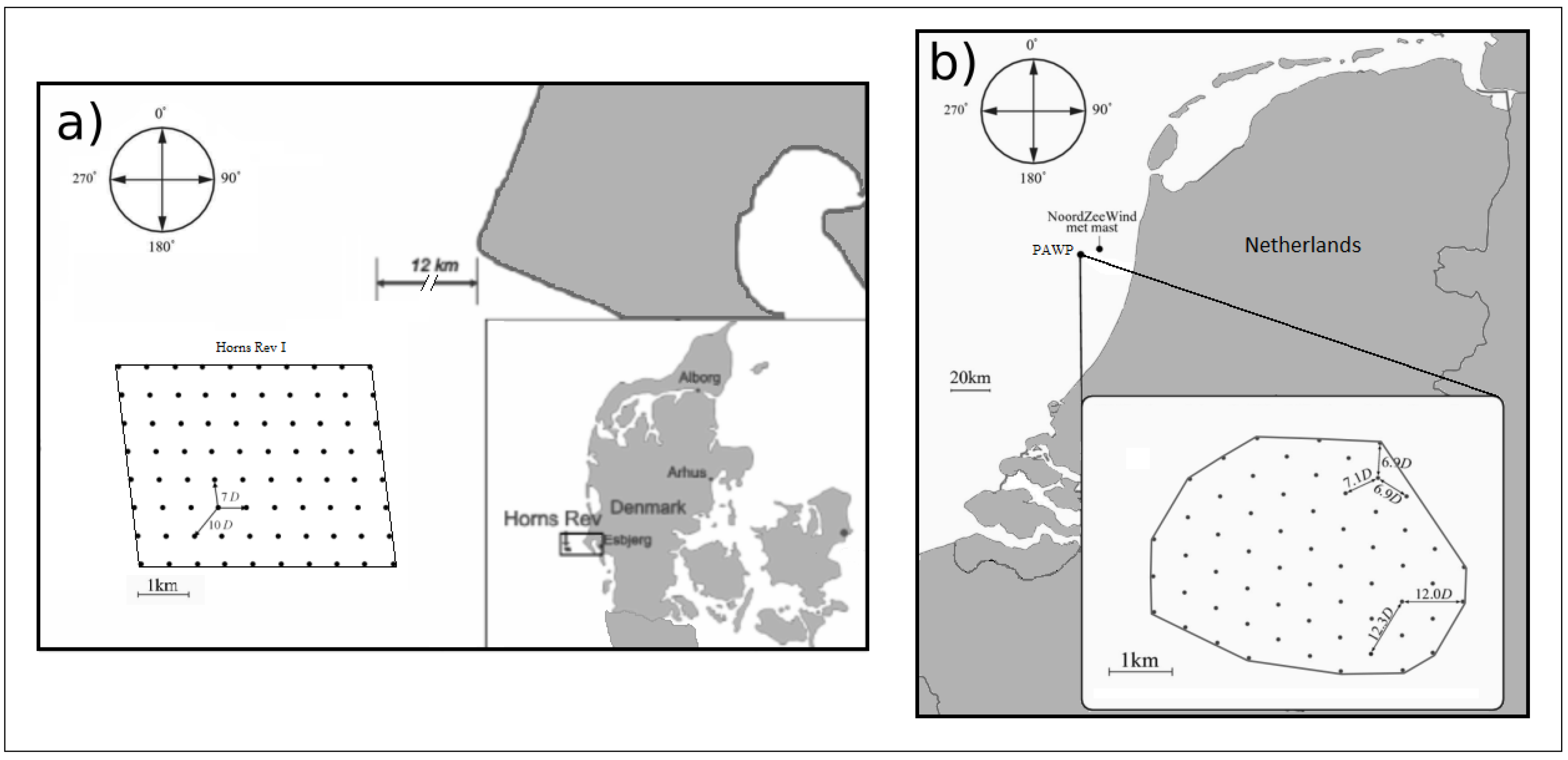
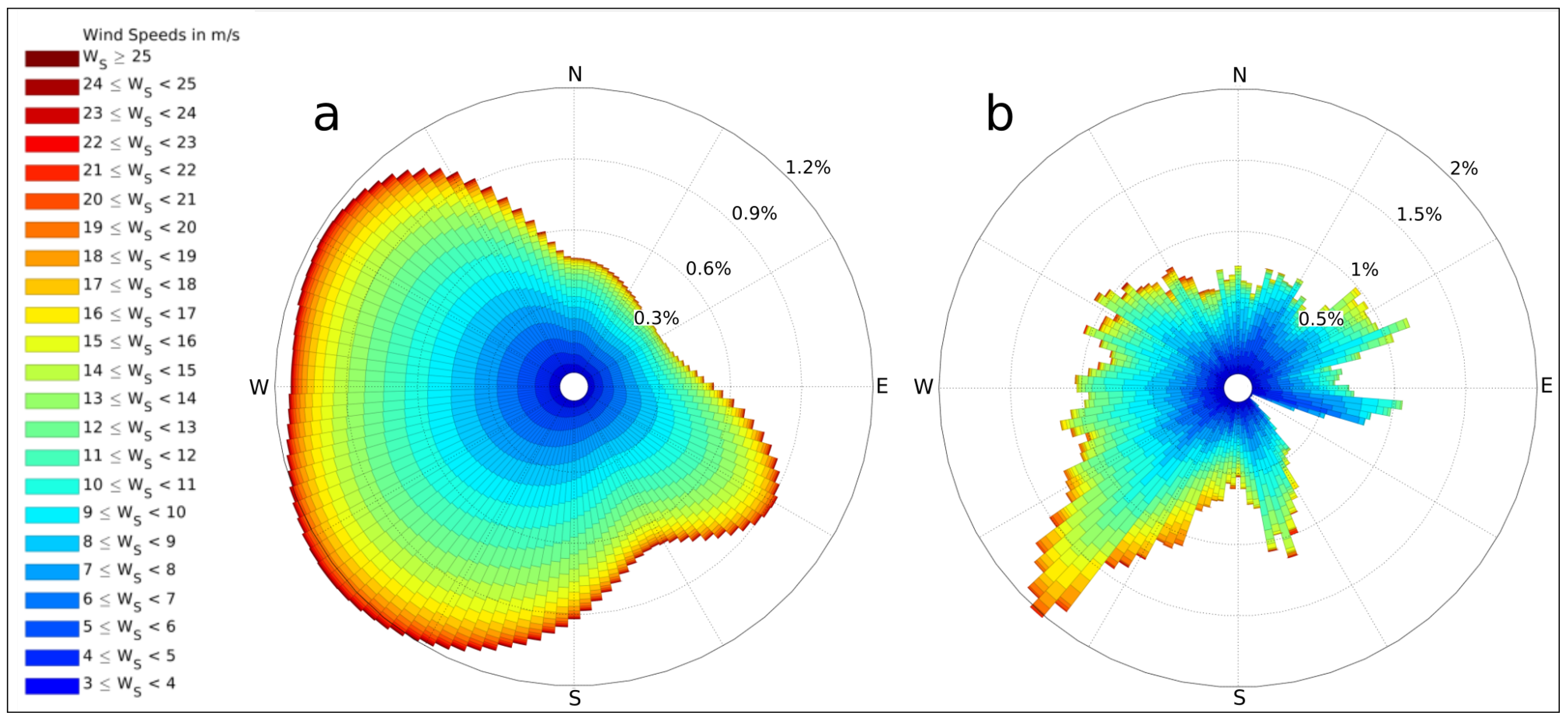
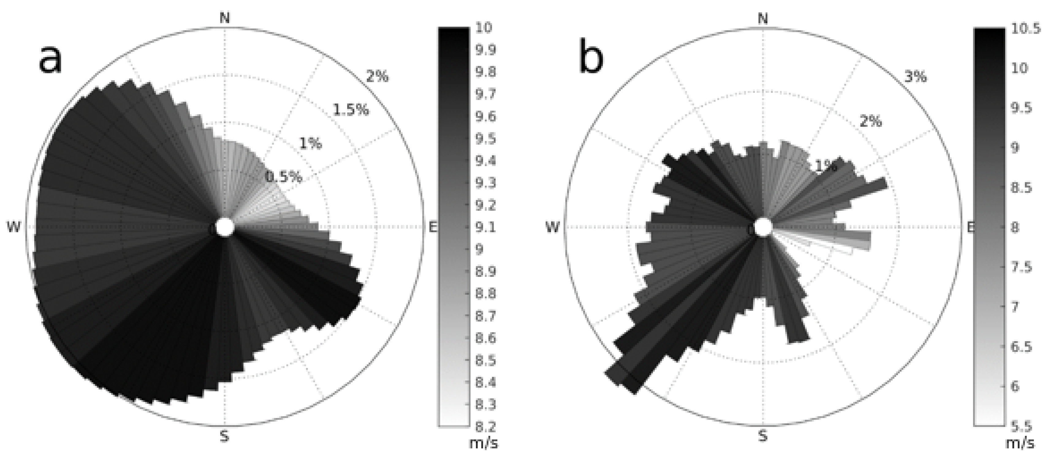
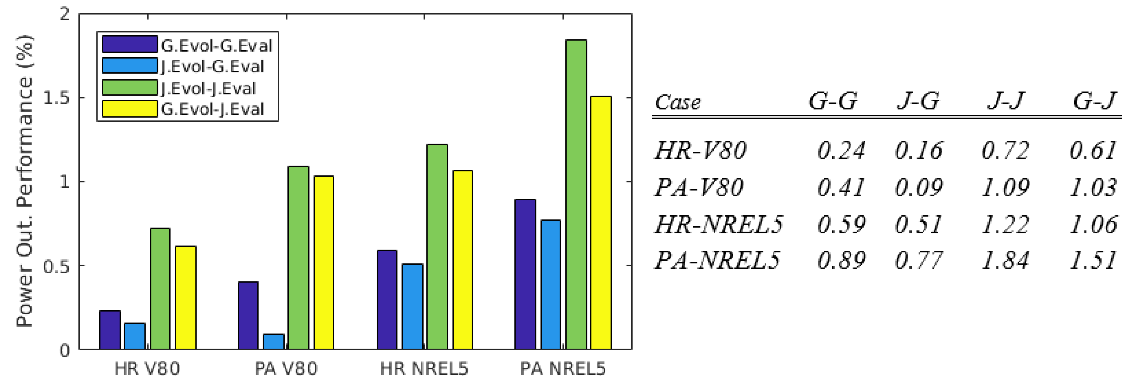
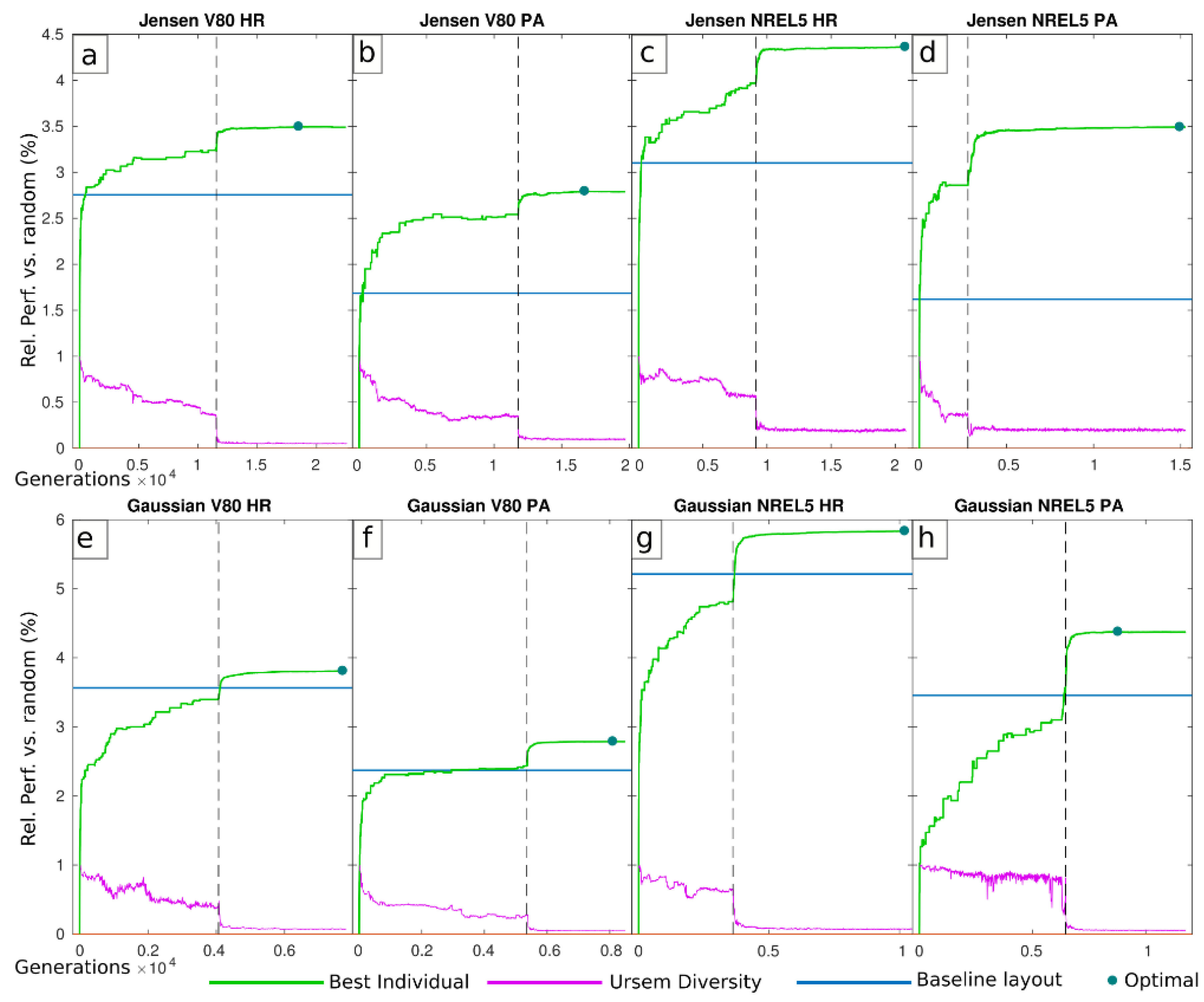
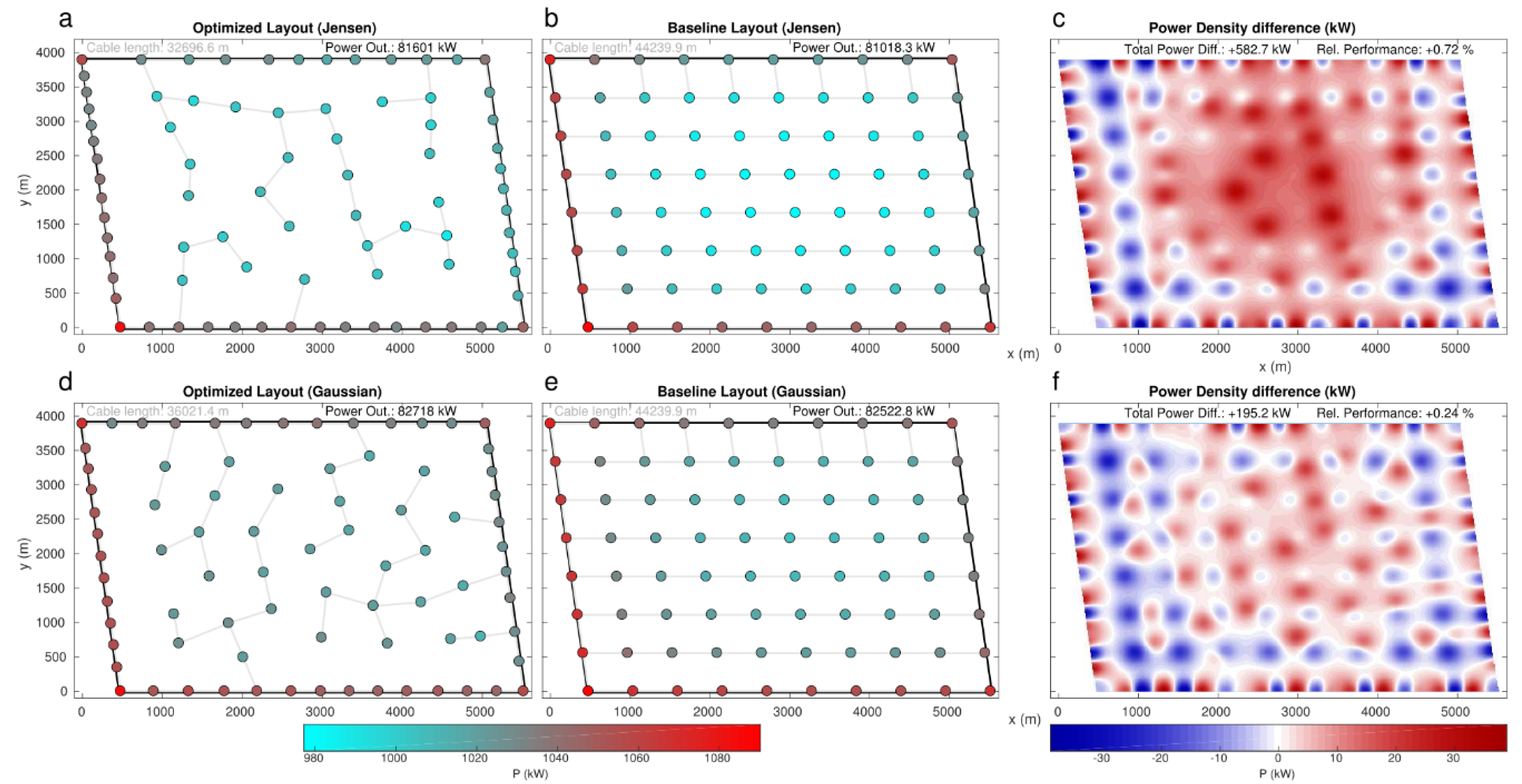
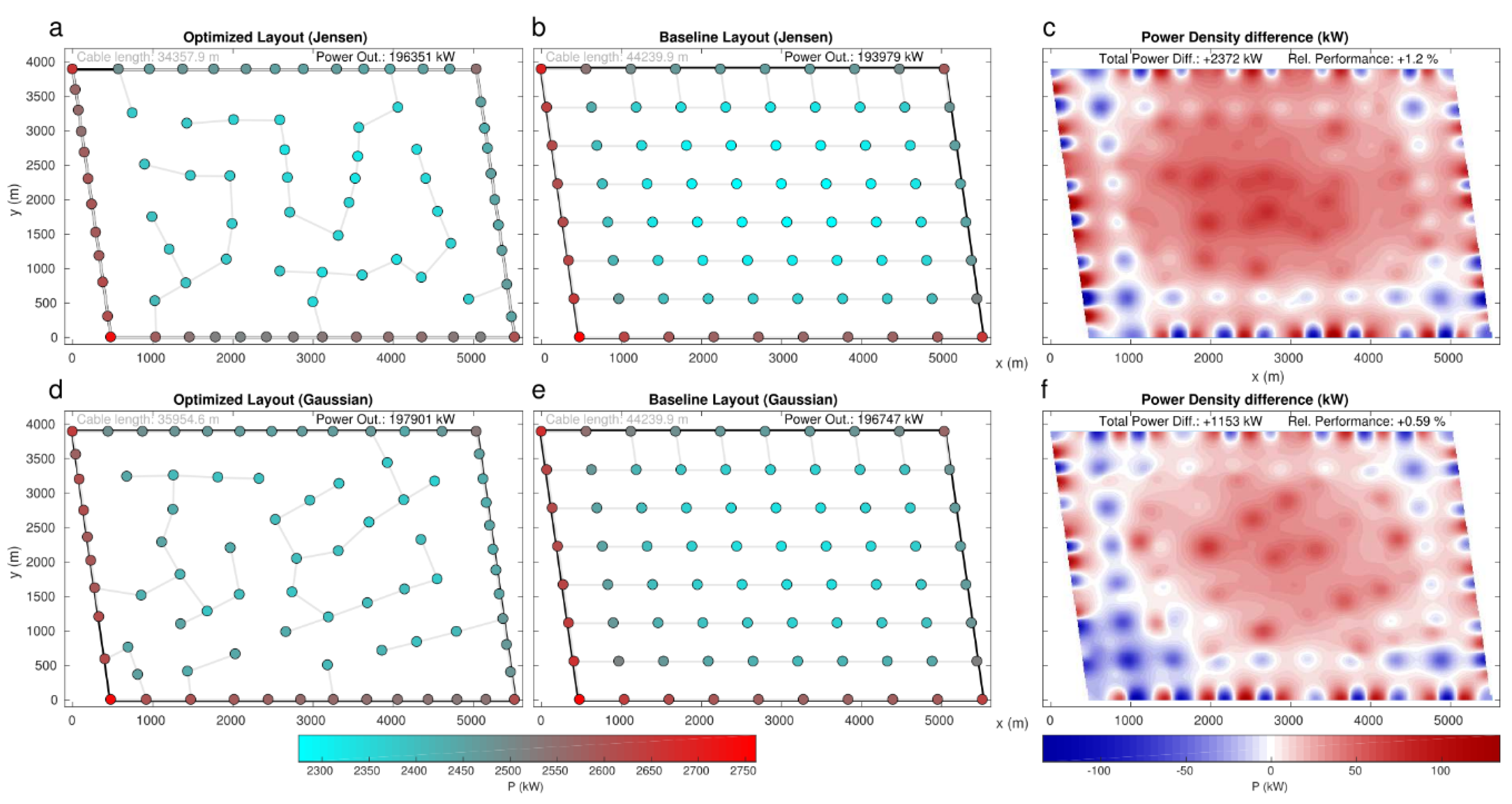
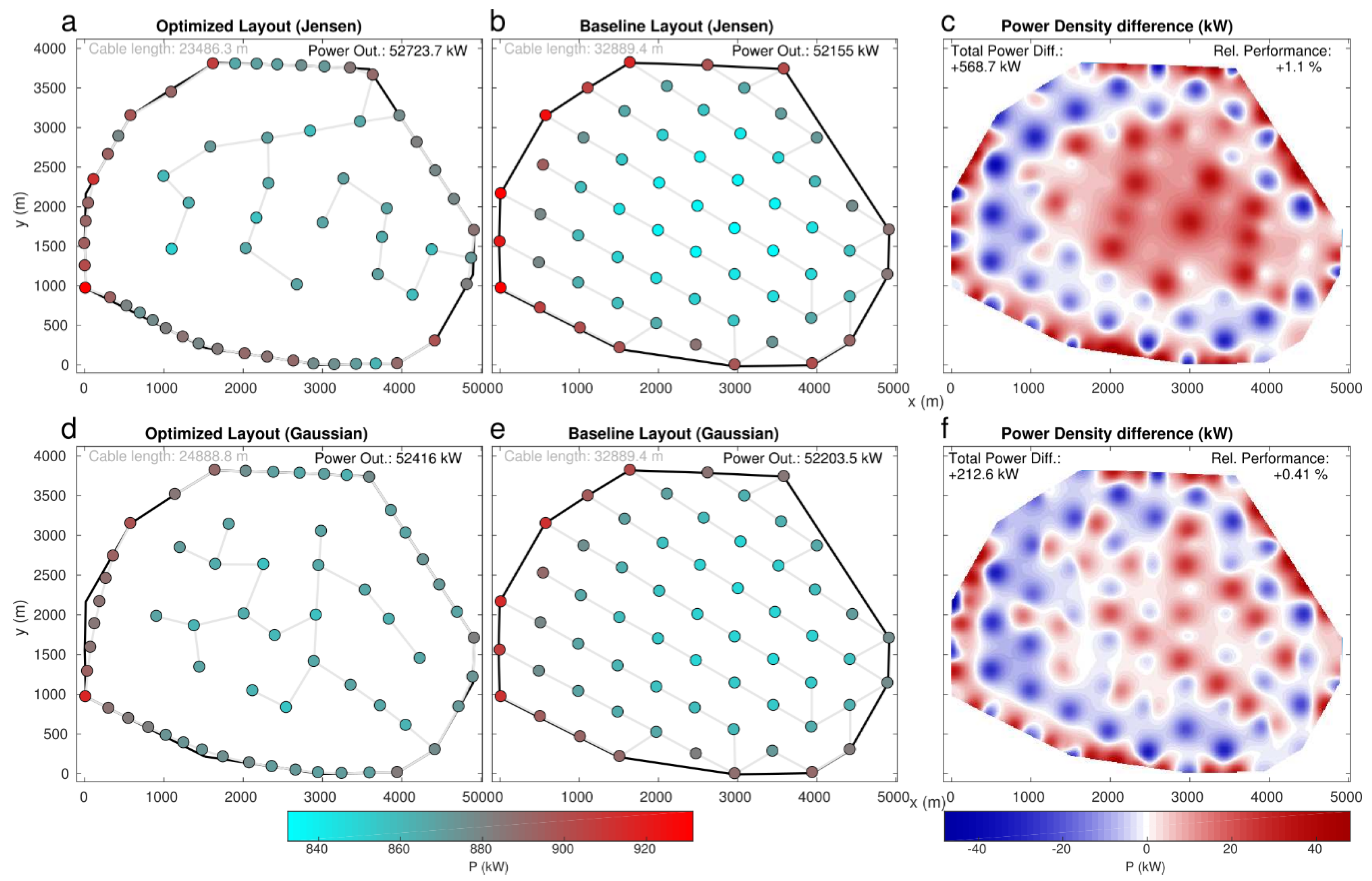
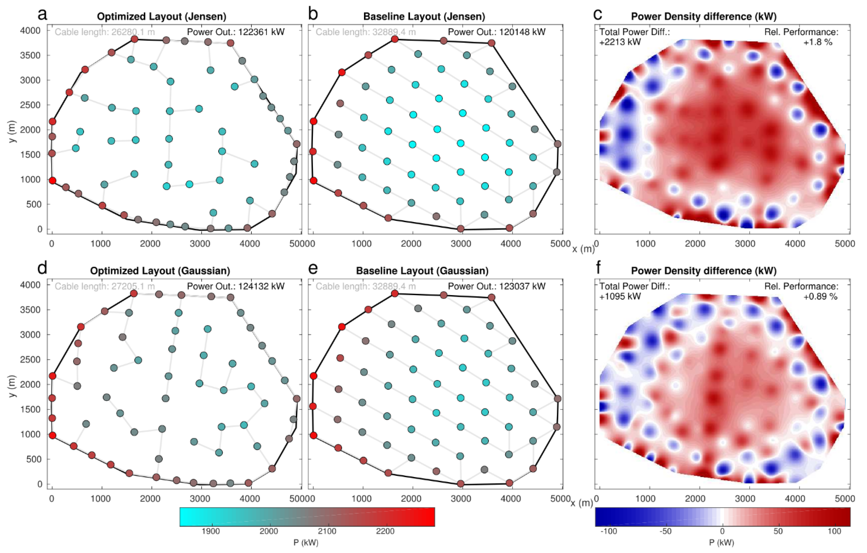
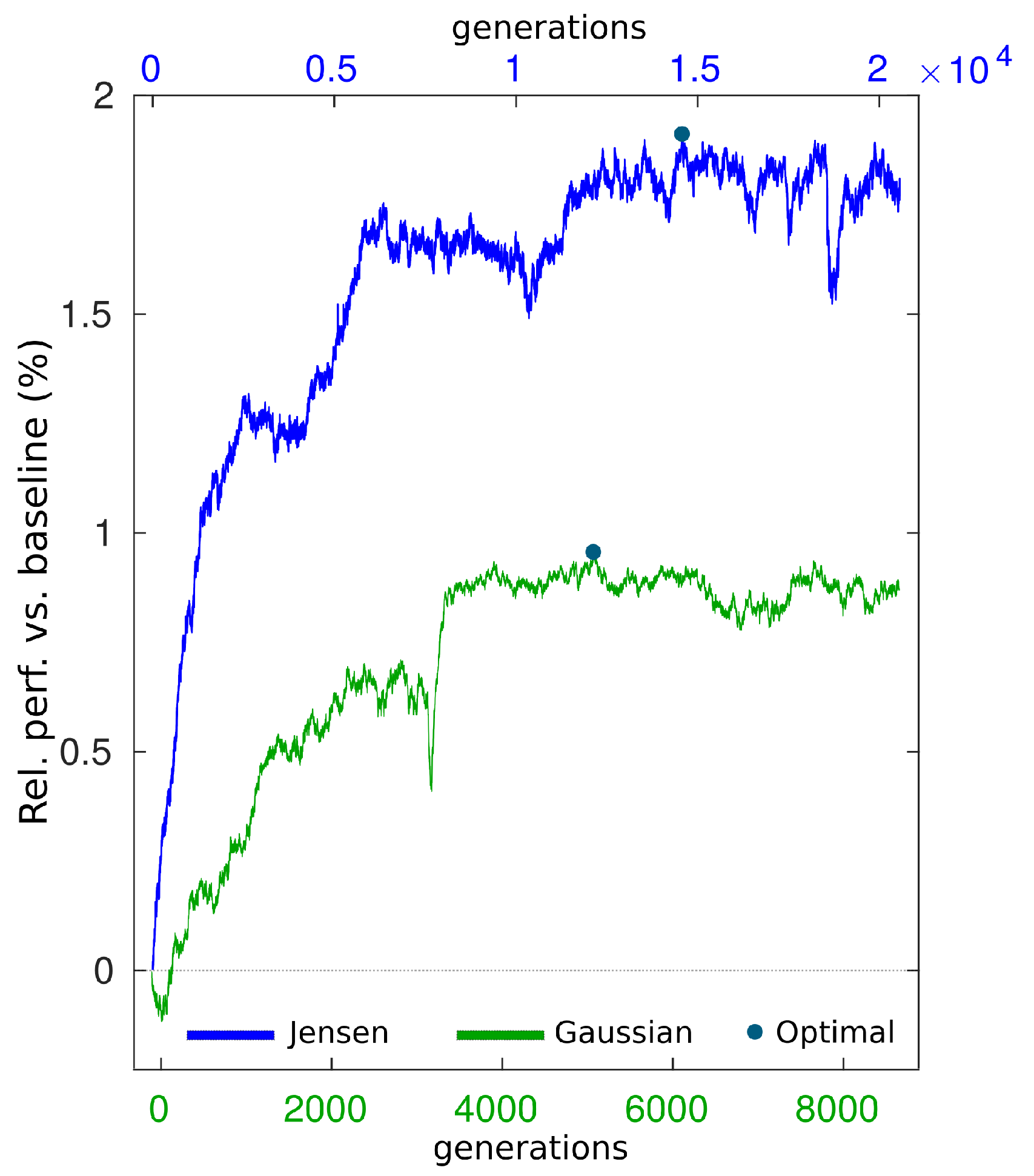
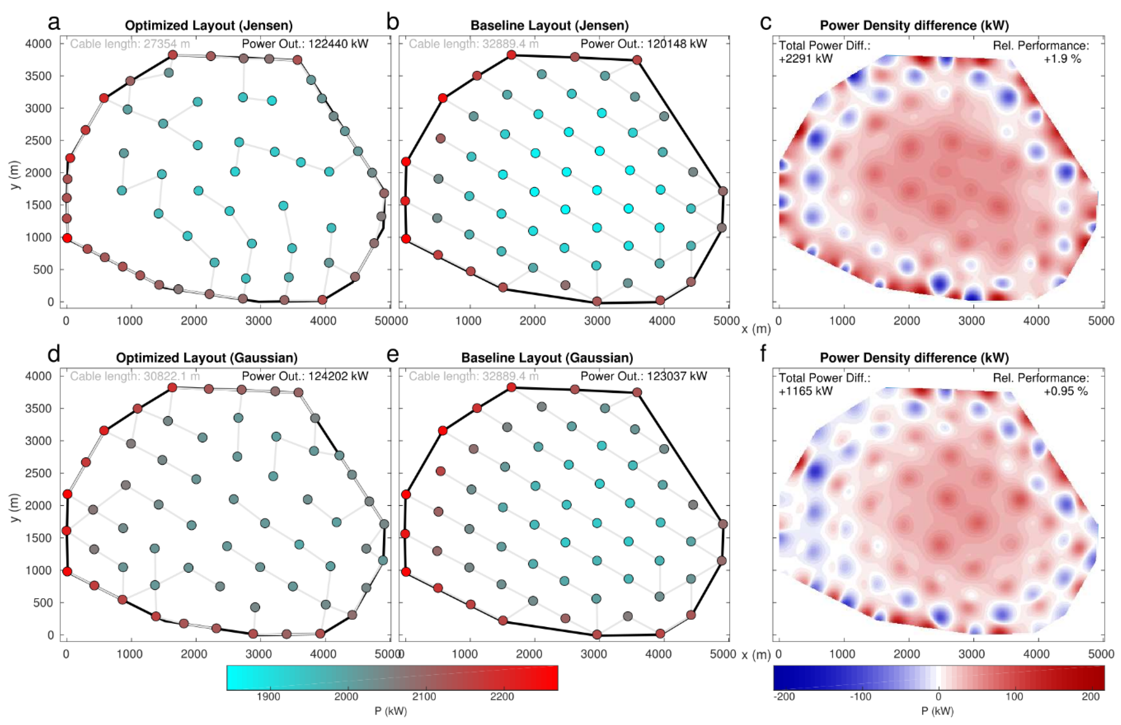
Table 1.
Summary of the main baseline features for the four wind farms considered.
| HR-V80 | HR-NREL5 | PA-V80 | PA-NREL5 | |
|---|---|---|---|---|
| Amount of Turbines | 80 | 80 | 60 | 60 |
| Hub Height (m) | 70 | 90 | 59 | 90 |
| Mast Height (m) | 62 | 62 | 70 | 70 |
| Rotor Diameter, D (m) | 80 | 126 | 80 | 126 |
| Turbine Rated Power | 2 MW | 5 MW | 2 MW | 5 MW |
| Gridded distance between turbines (m) | 7 D | 4.44 D | ∼7 D | ∼4.44 D |
Table 2.
Obtained selection pressure for CEGA according to the case considered.
| HR-V80 | HR-NREL5 | PA-V80 | PA-NREL5 | |
|---|---|---|---|---|
| 1.0008 | 1.002 | 1.0008 | 1.002 | |
| 0.02 | 0.02 | |||
| 1.00075 | 1.002 | 1.00075 | 1.002 | |
| 0.02 | 0.02 |
Table 3.
Obtained selection pressure for BLEA according to the case considered.
| HR-V80 | HR-NREL5 | PA-V80 | PA-NREL5 | |
|---|---|---|---|---|
| 1.00015 | 1.002 | 1.0001 | 1.0001 | |
Table 4.
Number of generations, transition generation (Pt), cause for transition (diversity decay, , or improvement stagnation, ) and computing time (), for the evolutions of the four cases and two wake models considered.
Table 4.
Number of generations, transition generation (Pt), cause for transition (diversity decay, , or improvement stagnation, ) and computing time (), for the evolutions of the four cases and two wake models considered.
| Jensen | HR-V80 | HR-NREL5 | PA-V80 | PA-NREL5 |
|---|---|---|---|---|
| Generations | 22,461 | 19,713 | 20,835 | 15,270 |
| Pt | 11,541 | 11,774 | 9137 | 2794 |
| Transition | Ud | Stag | Stag | Stag |
| C.time (s) | 7.60 | 5.83 | 7.50 | 6.82 |
| Gaussian | ||||
| Generations | 7792 | 8496 | 10,246 | 11,757 |
| Pt | 4070 | 5358 | 3612 | 6458 |
| Transition | Ud | Stag | Stag | Ud |
| C.time (s) | 1.45 | 0.94 | 1.86 | 1.46 |
Table 5.
Relative improvement (%) of the power output for the obtained BLEA layouts after evaluation with evalWR ( 1 ms resol.).
Table 5.
Relative improvement (%) of the power output for the obtained BLEA layouts after evaluation with evalWR ( 1 ms resol.).
| Case | Jensen | Gaussian |
|---|---|---|
| HR-V80 | 0.15 | 0.03 |
| PA-V80 | 0.63 | 0.28 |
| HR-NREL | 1.06 | 0.11 |
| PA-NREL | 1.91 | 0.95 |
© 2018 by the authors. Licensee MDPI, Basel, Switzerland. This article is an open access article distributed under the terms and conditions of the Creative Commons Attribution (CC BY) license (http://creativecommons.org/licenses/by/4.0/).
Share and Cite
MDPI and ACS Style
Kirchner-Bossi, N.; Porté-Agel, F. Realistic Wind Farm Layout Optimization through Genetic Algorithms Using a Gaussian Wake Model. Energies 2018, 11, 3268. https://doi.org/10.3390/en11123268
AMA Style
Kirchner-Bossi N, Porté-Agel F. Realistic Wind Farm Layout Optimization through Genetic Algorithms Using a Gaussian Wake Model. Energies. 2018; 11(12):3268. https://doi.org/10.3390/en11123268
Chicago/Turabian StyleKirchner-Bossi, Nicolas, and Fernando Porté-Agel. 2018. "Realistic Wind Farm Layout Optimization through Genetic Algorithms Using a Gaussian Wake Model" Energies 11, no. 12: 3268. https://doi.org/10.3390/en11123268
Note that from the first issue of 2016, this journal uses article numbers instead of page numbers. See further details here.