Prediction of Wave Power Generation Using a Convolutional Neural Network with Multiple Inputs

1
National Ocean Technology Center, Tianjin 300112, China
2
Engineering Department, Lancaster University, Bailrigg, Lancaster LA1 4YW, UK
*
Author to whom correspondence should be addressed.
Energies 2018, 11(8), 2097; https://doi.org/10.3390/en11082097
Submission received: 26 May 2018
/
Revised: 27 June 2018
/
Accepted: 28 June 2018
/
Published: 13 August 2018
(This article belongs to the Section F: Electrical Engineering)
Abstract
:Successful development of a marine wave energy converter (WEC) relies strongly on the development of the power generation device, which needs to be efficient and cost-effective. An innovative multi-input approach based on the Convolutional Neural Network (CNN) is investigated to predict the power generation of a WEC system using a double-buoy oscillating body device (OBD). The results from the experimental data show that the proposed multi-input CNN performs much better at predicting results compared with the conventional artificial network and regression models. Through the power generation analysis of this double-buoy OBD, it shows that the power output has a positive correlation with the wave height when it is higher than 0.2 m, which becomes even stronger if the wave height is higher than 0.6 m. Furthermore, the proposed approach associated with the CNN algorithm in this study can potentially detect the changes that could be due to presence of anomalies and therefore be used for condition monitoring and fault diagnosis of marine energy converters. The results are also able to facilitate controlling of the electricity balance among energy conversion, wave power produced and storage.
1. Introduction
Increases in energy demand and recent concerns regarding climate change necessitate developing reliable and alternative energy technologies in order to make society’s development sustainable. Wave energy, as an enormous potential and inexhaustible source of energy, still remains widely untapped [1]. Until now, a variety of wave energy devices have bloomed based on different types of technologies. Most of them absorb energy from the wave height and the water depth. The location for a WEC system typically include shoreline, near-shore and offshore [2]. With the contribution from the improved technological support, various types of concepts/prototypes to extract wave energy from ocean have emerged in recent years. However, the technical level is still in an immature stage [3]. In other words, despite the high technology readiness level (TRL) achieved by some devices (level eight) [4], their commercial readiness still needs to be proven. Following the pace of offshore wind energy development, it is a priority to understand the operation and performance of WECs in order to progressively demonstrate these devices under ocean conditions and increase electricity generation. The performance was considered as not only for redesign, but also for operation and maintenance.
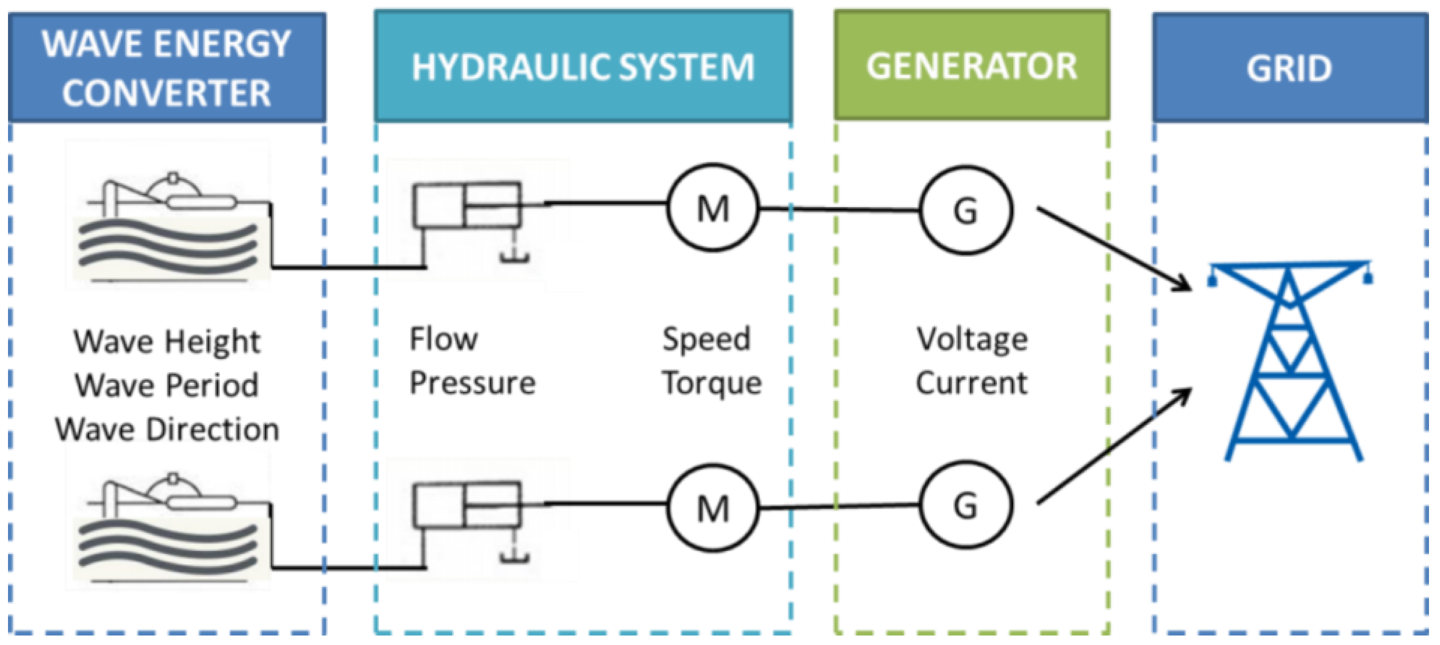
So far, more than 1000 WECs have been patented worldwide. They can be classified into three categories [5]: oscillating water column (OWC) devices [6], oscillating body systems [7], and overtopping converters [8]. Among them, a mechanical interface is required to convert the intermittent multi-direction motion into a continuous one-direction motion and the hydraulic motors represent one of the most frequently equipped transmissions in the oscillating body systems [9]. The schematic diagram of a typical hydraulic oscillating body system is shown in Figure 1. A WEC is typically formed by three stages when converting wave energy into electrical energy. This includes (a) a front interface, the portion of a device that directly interacts with the incident waves, (b) a power take-off (PTO) system used to transform the front-end energy into other forms of energy, like mechanical energy, and (c) an electrical energy generation system that takes the responsibility to do the final conversion. In the wind energy industry, the supervisory control and data acquisition (SCADA) system, which records hundreds of variables related to operational parameters, is installed in most modern wind farms [10]. Compared with wind turbines, the data available from WECs are not as abundant in quantity because of the presently immature ocean wave technologies. However, it is worth mentioning that acquiring data from the operating WECs is more difficult than the wind turbines because of not only the harsh ocean conditions but also the high cost.
In the operation and performance domain, a reliable power forecast plays a crucial role in reducing the need of controlling energy, integrating the highly volatile production, planning unit commitment, scheduling and dispatching by system operators, and maximizing advantage by electricity traders. In addition, the accurate prediction of wave loads, motion characteristics and power requirements are significantly important for the design of WEC converters [11]. For the grid, the accurate prediction of wave energy is considered as a major improvement of reliability in large-scale wave power integration and of managing the variability of wave generation and the electricity balance on the grid. As a result, monitoring and predicting the power output of the WEC system based on sensor data from each part of the system become increasingly valuable. The fast growth of machine learning (ML) and deep learning technologies associated with statistical analysis give wings to the forecast and evaluation.
Traditionally, wave height and direction can be forecast by either statistical techniques or physics-based models [12,13]. There are many examples of the wave forecast system based on physical models. For example, the European Centre for Medium-Range Weather Forecast (ECMWF) and the WAVEWATCH-III organizations have performed predictions using wind data from the Global Data Assimilation Scheme (GDAS), Ocean weather and Gulf of Mexico [14]. The statistical approaches such as neural networks and regression-based techniques have also made great progresses [15]. By contrast, the physics-based wave forecasting models are widely used due to the mature technology and adequate historical data. Wave prediction can take advantage of opportunities from the rapid development in recent years of wind power prediction. Many algorithms, approaches and methods have been developed in the statistical model domain in renewable energy prediction, such as wind power and solar power prediction. So far, artificial neural network (ANN) methodology has been applied to predict short–mid-term solar power for a 750 W solar photovoltaic (PV) panel [16]. A least-square (LS) support vector machine (SVM)-based model was applied for short-term forecasting of the atmospheric transmissivity, thus determining the magnitude of solar power [17]. Very short-term wind power predictions problems were addressed in the wind power industry by developing the neural network (NN) model and the SVM, boosting tree, random forest, k-nearest neighbour algorithms [18,19]. The data-based models with wind speed, wind generator speed, voltage and current in all phases as inputs could achieve an accurate prediction of the wind power output [20]. For medium-term and long-term wind power prediction, ANN models, adaptive fuzzy logistic and multilayer perceptrons are the most popular kinds of methods [21,22,23]. Moreover, as the deep learning algorithms bloom, the CNN, long short term memory (LSTM), Deep Brief Net (DBN) and recurrent neural network (RNN) modelling have become popular in some renewable energy predictions. A deep RNN was modelled to forecast the short-term electricity load at different levels of the power systems. Deep multi-layered neural model has been reported to evaluate the electricity generation output from a wind farm 1 day in advance. A novel hybrid deep-learning network associated with an empirical wavelet transformation and two kinds of RNN was employed to make the accurate prediction of the wind speed and wind energy [24,25,26].
The primary intention of this work is to illustrate the power prediction and performance of a hydraulic WEC operating in the open sea condition for more than two months based on statistical analysis and physical modelling technologies. A multi-input approach based on CNN is presented to predict the power output at a particular coastal area. The CNN network reaches considerable achievement in terms of image and video recognition as well as language processing. One of the novelties is that the algorithms capable of converting the multi-input time series data into 2-dimension (2D) images play a unique role in the construction of CNN model. The performance turns out to be remarkably better than other models, indicating its strong feasibility and suitability for power prediction. In addition, the connection between converter, hydraulic system, generator, and the grid will be clarified through analysing the wave, hydraulic motor pressure, and electrical data.
For this purpose, this paper is organized as follows: Section 2 gives the details of the device and the measurement datasets used in the paper and presents the performance of the WEC. Section 3 describes the methodology of CNN algorithm in details. In Section 4, performance and results of the proposed model are presented. Finally, Section 5 summarizes the conclusions from the study.
2. Operation and Performance Analysis
2.1. Data Acquisition
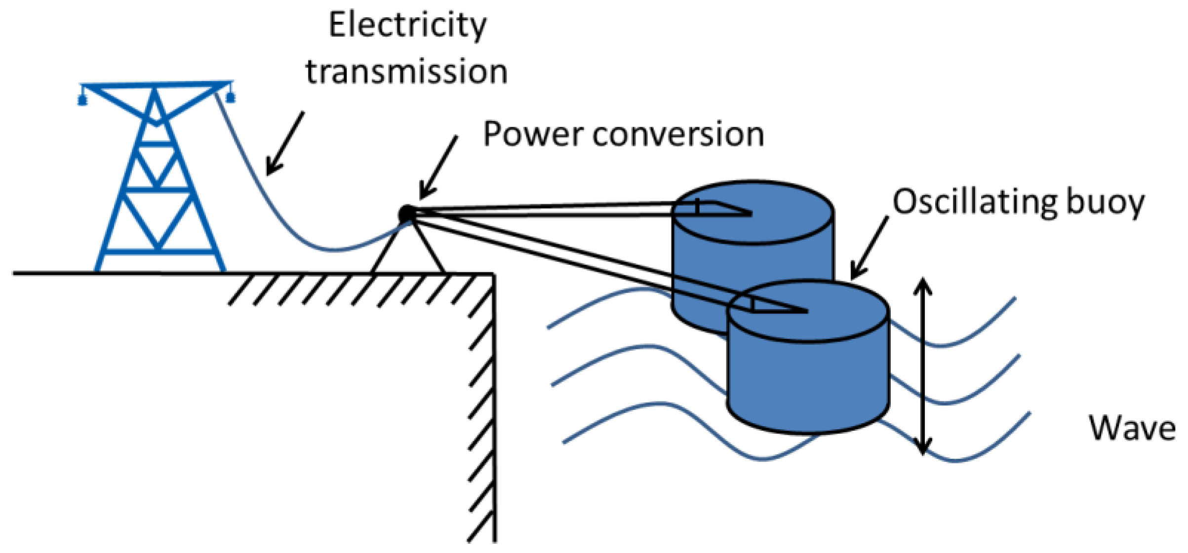
Normally, there are three conversion stages to extract wave energy from the ocean. These include: (a) capture of the kinetic energy by the power capture system of WEC, (b) conversion into mechanical energy by the PTO and then into electrical power by generators, such as direct-drive linear generators; (c) storage of the electricity in batteries or transport to a grid. The data used in this study were acquired from a demonstration WEC deployed in open sea conditions in a near-shore area. This WEC contains data from a double-buoy hydraulic OBD with ten kW level capacity collected from February to April 2017. As shown in Figure 2, the WEC contains an oscillating buoy system and comprises of four main parts, i.e., power capture, hydraulic motor, generator and power transmission. The oscillating buoy captures kinetic energy through its up-and-down motions of the ocean waves. The hydraulic motor and generator are responsible for converting the kinetic energy into electricity and transfer it to land through a sea cable. In the first conversion, the wave energy is captured by two oscillating buoys while a hydraulic pressure system is deployed in the second conversion. The power capture system uses hydraulic rams installed inside the two oscillating buoys. This 10 kW WEC prototype was invented by a research institution in 2016 and underwent its first sea tests at a testing station in SanYa, Hainan Province, China in 2017. The two oscillating buoys were installed on the edge of a dock side by side where they were fixed together and moved up and down simultaneously according to the wave conditions. The wave conditions in this area change significantly during the different seasons. The simulation data from the numerical model show that the mean wave height reaches 0.7 m in summer with a major south direction. The wave height in winter is much higher than in summer, with a 2.0 m maximum height and a northeast direction [27]. The real wave heights were observed by an optical wave meter and recorded daily every 4 h from 8:00 to 18:00 from February to April 2017. The real data show the maximum wave height was approximately 1.1 m during the observation period.
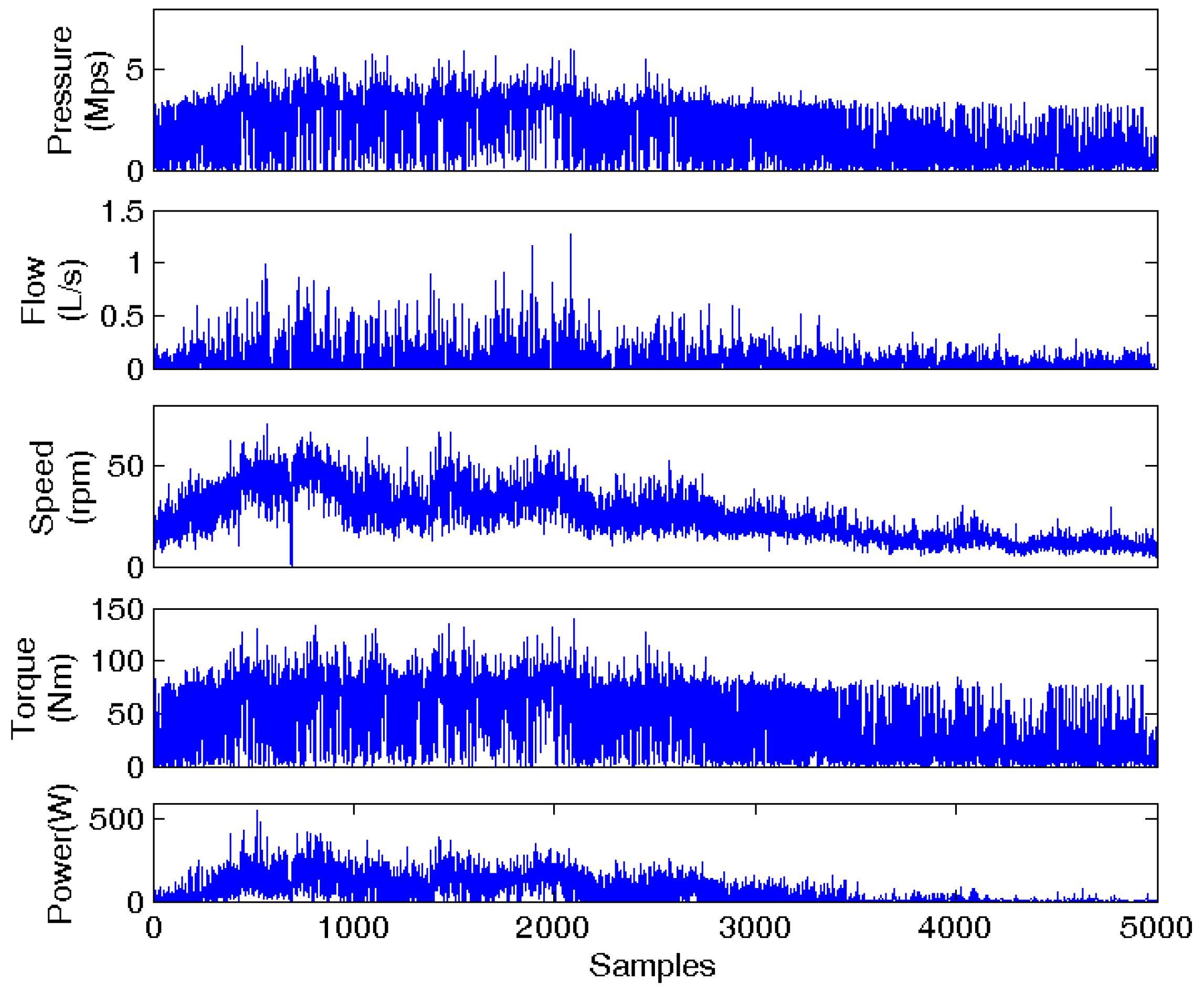
Approximately 20 readings for various pressures, speed, voltage and current signals were recorded at a one-minute interval. These readings were classified into three groups: resource data, hydraulic data and electrical data. In the hydraulic group, the four readings (hydraulic flow, hydraulic pressure, motor speed and motor torque) are most significantly associated with the power output and will be used in the study. The pre-process of data is necessary to eliminate digital and constant signals and filter out those data collected when the WEC is inactive or abnormal. There are gaps existed between the data normally because the generator is inactive. These occasions may be caused by the periods of low wave energy and harsh condition; some abnormal values within the data caused by disturbing signals and power failure also need to remove. Figure 3 shows the measurement data of these four variables after pre-processing.
2.2. Power Curves
The extraction energy efficiency of wave energy varies wildly for different WECs because of the individual technology features. Typically, the extraction energy efficiency between the wave resource and hydraulic system can be calculated by dividing the wave resource by the power achieved by the hydraulic system, which depends on the level of maturity of the devices. The wave resource can be calculated by the equation below:
where stands for the power input from wave power, stands for the density of sea water, stands for the acceleration of gravity, stands for the wave height in zero-order moment of the spectral function. Since the wave period were not been measured during the testing, present method uses the (energy period) as a period parameter, defined as:
where stands for the minus-one spectral moments, stands for the zeroth spectral moments [28,29].
The input and output power of the hydraulic system can be calculated by Equations (3) and (4) respectively:
where stands for the input power of the hydraulic system; stands for pressure and stands for the flow.
where stands for the power output of the hydraulic system; stands for torque and stands for speed.
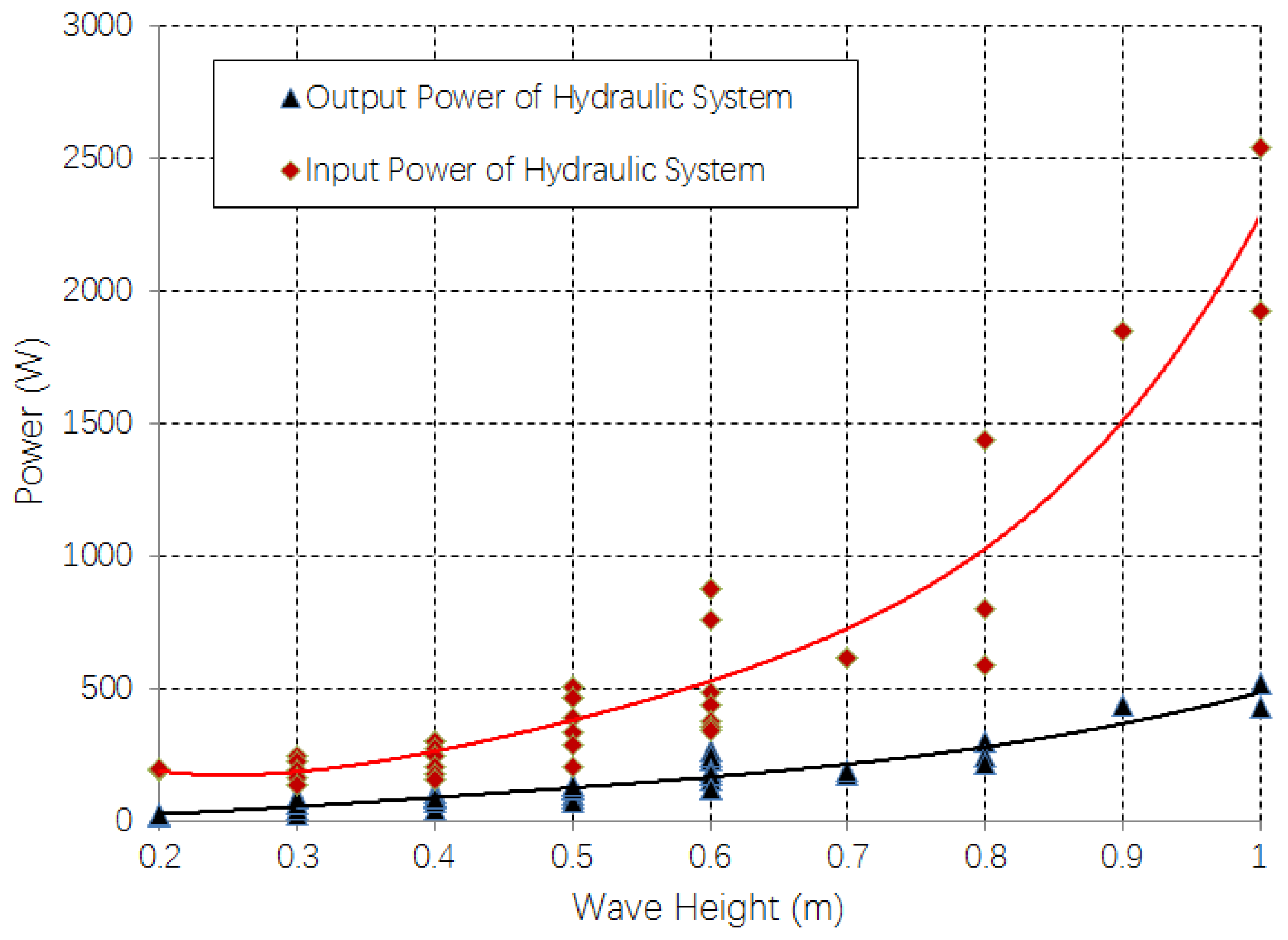
With the wave height, input and output power of the hydraulic system being known, the wave-power curves of this device can be drawn, elaborating the relationship between wave height and active power output from the hydraulic system, as illustrated in Figure 4. The green dots denote the input power while the blue dots represent the power output. It can be observed that both the power input and output tend to maintain a positive correlation with the wave height when it is higher than 0.2 m. The positive correlation diverges when the wave height is higher than 0.6 m. In general, these trends coincide with calculations using the wave energy [30] that varies with the square of wave height. It can also be seen that the device remains inactive when the wave height is below approximately 0.25 m, indicating the start wave height of this device is 0.25 m. When comparing these two power curves, it is found that the efficiency from wave energy to hydraulic power output shows little difference between 0.2 m and 0.6 m. Nevertheless, it increases smoothly when the wave height is higher than 0.6 m; this could reveal the mechanism of input and output power efficiency of this particular device.
2.3. Energy Conversion Efficiency
The efficiency of a PTO system is vital to determine the stability and reliability of the device. Of the current WEC concepts developed so far, 42% use hydraulic systems to increase the overall efficiency of the converters and the electric performance [31]. For this WEC, the efficiencies from three parts, i.e., hydraulic system, electrical generator and electricity storage, were evaluated using historical data. The data were averaged every 4 h for an entire day of 24 h (six groups’ data each day). The average efficiency of the hydraulic system is calculated by . Here, P represents the average conversion efficiency from the power input while represents the average conversion efficiency from the power generation.
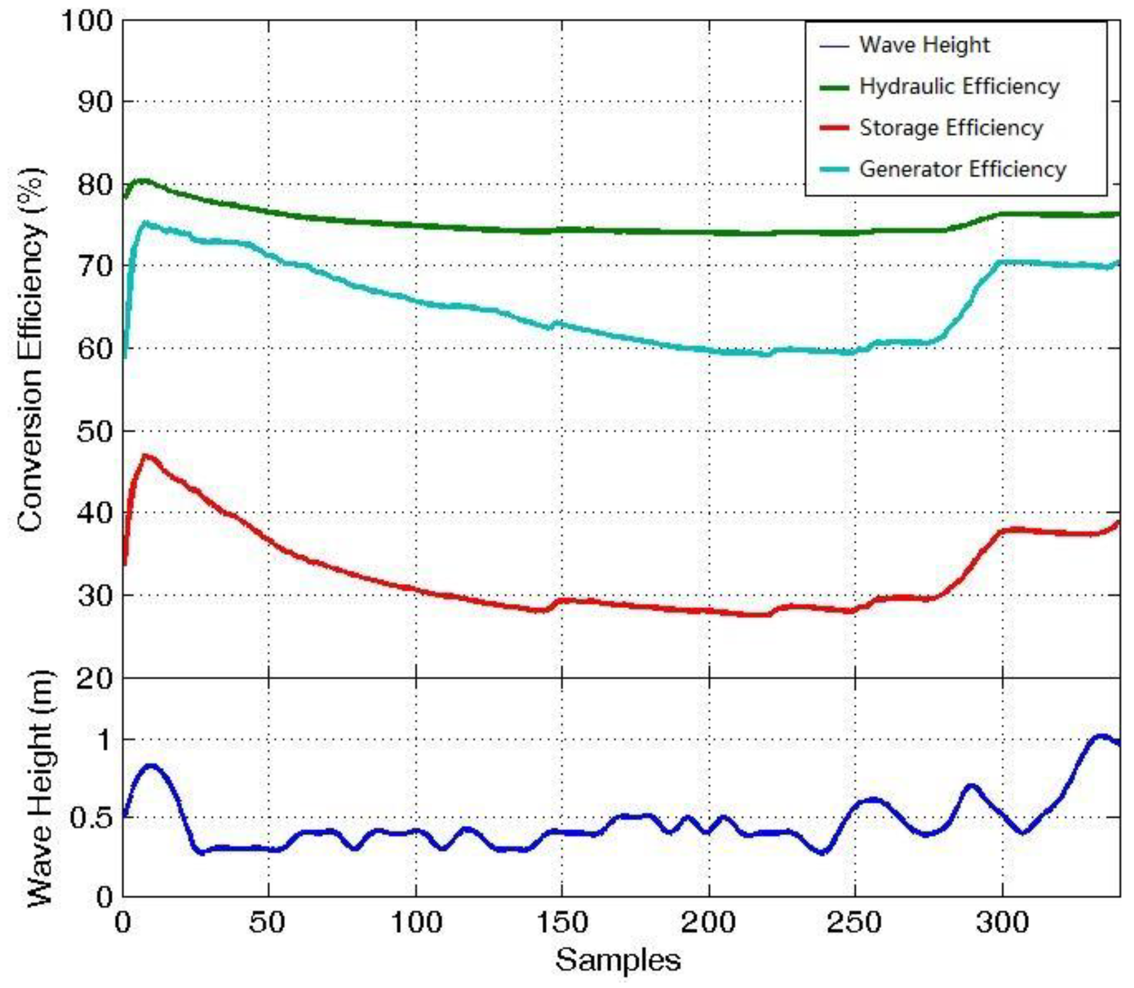
It can be seen from Figure 5 that the efficiencies of the hydraulic system, electrical generator and electricity storage show similar tendencies. The hydraulic system demonstrates the highest efficiency between 70% and 80% during the hydraulic conversion. The electrical storage efficiency is slightly lower than that of the hydraulic system, between 60% and 75%. The electrical generator consumes the largest proportion of the energy and remains at 30% to 45% efficiency. Evidently, all three efficiencies grow rapidly following the peak of wave height nearby 10 m at 300 samples. The discrepancy between 300 and 350 samples might be due to shortness of the wave direction and data period. It is considered that the high efficiency level may be caused by the wave period, which is appropriate for the converters. The wave direction also causes variation of the energy efficiency because the geographic terrain and conditions can amplify the wave height and concentrate wave energy on a particular position [32]. The curves also suggest that the generating conversion has the greatest potential for improvement.
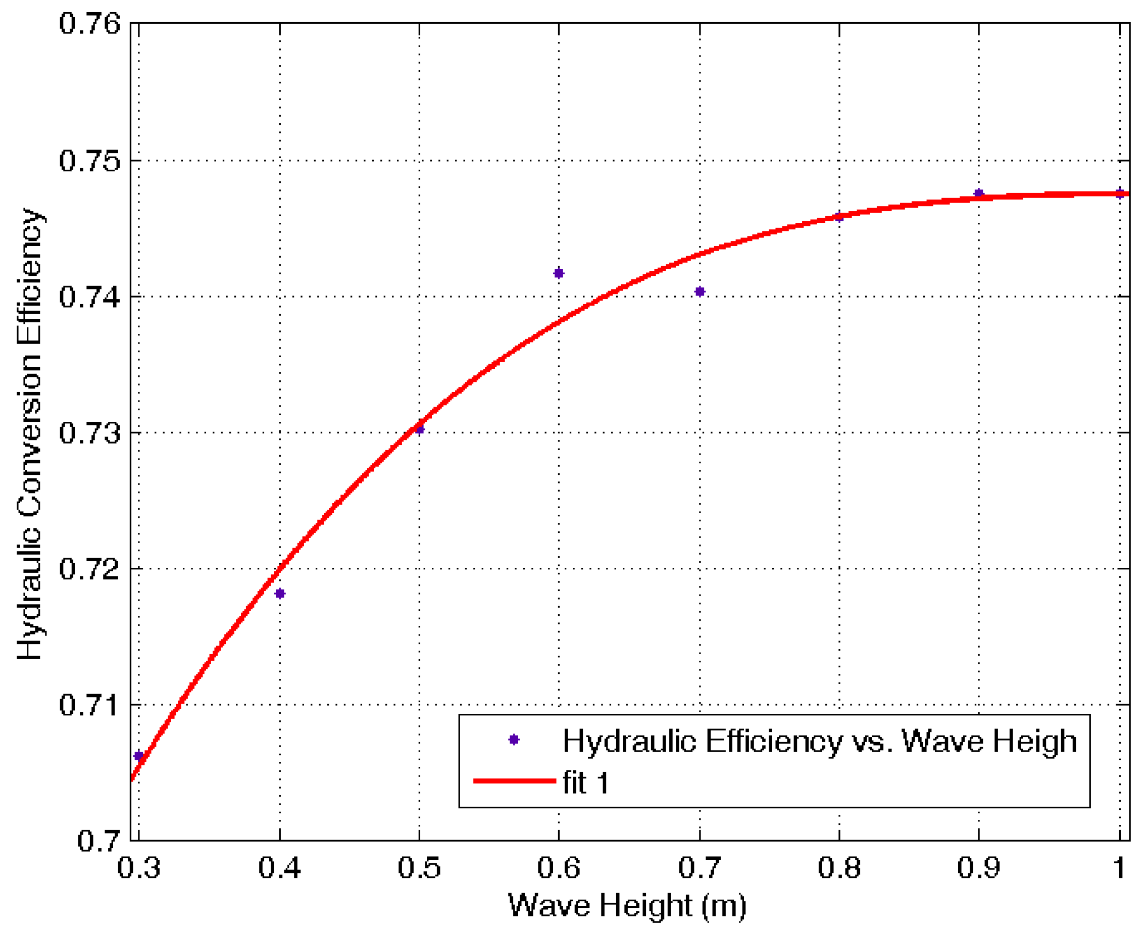
Finally, the wave height-efficiency curve can be drawn, as shown in Figure 6, which successfully shows the correlations between the wave height and the hydraulic power. It is observed that the hydraulic conversion efficiency increases sharply as the wave height grows at the beginning. The change gradient becomes low when the wave height increases to between 0.5 m and 0.8 m, and it remains almost stable after 0.8 m. The curve also illustrates some of the most important characteristic of this WEC, such as the start wave height and rated wave height.
3. Methodology
3.1. Convolutional Neural Networks
Due to the 1-dimension (1D) time series data from WEC may ignore vital information between time intervals, we applied a novel CNN algorithm, which convert 1D input data into 2D images. Traditionally, autoregressive models (AM), Linear Dynamical Systems (LDS), and the popular Hidden Markov Model (HMM) represent the classic approaches for modelling sequential time series data. The parameters to be predicted are used as perceptual judgements and features to do the classification [33]. However, deep learning, which is derives from ML is able to learn high-level abstractions in data by utilizing hierarchical architectures [34]. As one of the deep learning algorithms, the CNN method has been considered one of the most appropriate methods to address the predicting problems. It has addressed plenty of problems in terms of sequential learning and shown its great potential in recent years [35]. The input and output data of the network observed in this paper is considered as a multiple data source, showing the connections between different parts of the device. The wave represents the original driver of the whole generation system, which could not be predicted accurately. This novel CNN approach shows advantages on prediction of the physical variables and makes considerable improvements in terms of the standard deviation and mean absolute values of the prediction performance. It also outperforms ML by a significant margin in forecasting stability and accuracy.
Different from the linear maps applied by ANNs, CNN considers a particular form of convolutional layers (or convolutional filters). Linear functions used by the convolutional filters convert the input data into images in a sliding-window fashion [36]. Among the many deep neural networks, the CNN demonstrates excellent performance in the field of image processing, which comprises convolutional layers, pooling layer, and fully connected layers [37]. In addition, there are many advantages to apply CNNs. This is because: (a) the connections of receptive fields are able to reduce plenty of parameters, (b) the replication of each filter shares the same parameters (weight vector and bias) and forms a feature map and (c) the diverse positions along the network are participated to compute features using convolution activations statistics [38,39].
3.2. Network Architecture
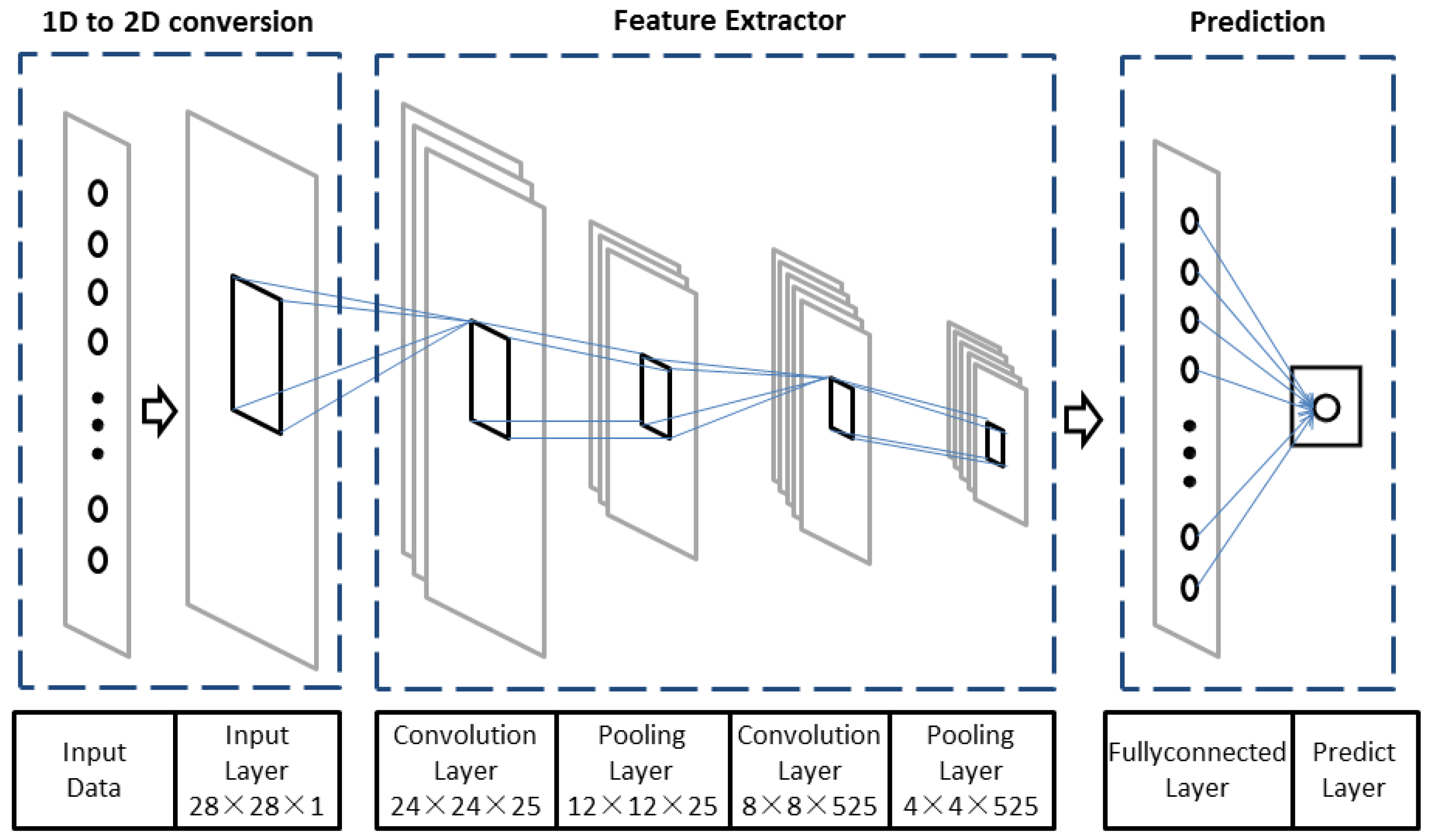
This network structure is formed by four hidden layers and the relevant hyper-parameters are shown in Figure 7. The values of the hyper-parameters used in the network are listed in Table 1. The input layer is four time series of observations collected from the hydraulic system of a WEC. The 1D to 2D conversion layer is used to rearrange one image set by the four series of observations mentioned in Section 2.1. The size of input layer is set to 28 × 28 pixels because 28 pixels are the default value of digital image in traditional CNN. The convolution layer performs convolution operations with the kernel size of 5 × 5 to acquire feature maps of the image. The dimension of the first convolution layer is set as 24 × 24 × 25, which convolutes an input image size from 28 × 28 pixels (25 layers set by experience). All the convolution layers are connected to the Rectified Linear Unit (ReLU) activation functions instead of sigmoid function because ReLU is faster and can reduce likelihood of vanishing gradient [40]. We use the max-pooling layer 2 × 2 and second convolution layers (5 × 5 kernel size and 25 layers as well). Finally, the dimension of the fully connected layer is set as 40, followed by a predict layer as required.
The activation function of the predict layer is a linear function (identity function, i.e., y = x) because the values are unbounded in terms of regression.
The CNN is trained using the least absolute deviations (L1) as the loss function to minimize the absolute differences between the jth target value and the jth estimated value of this network. The loss function L1 is defined as:
where n denotes the size of the dataset.
Convolution Layer
The convolution layer is comprised from a two-layer feed-forward NN. The NN uses a convolution algorithm to extract the feature maps from original image [41]. As mentioned above, the neurons in the same layer have no connections. But the neurons in different layers are deployed in order to simplify the feed forward process, as well as back propagation. Noticeably, the weights and feature map are convolved in the previous layer. An activation function is used to generate the current layer and output feature maps. The convolution layer is calculated as follows:
where xi,j denotes a specific element in the input image, wm,n denotes the weight in mth row nth column, wb represents bias of the filter, ai,j is the element of the feature map. Notice that the ReLU function is chosen as the output activation function f.
Pooling Layers
Pooling layers are typically used immediately after convolution layers to simplify the information. Traditionally, convolution layers associate with pooling layers for the sake of constructing stable structures and preserving characteristics. Another advantage of applying pooling layers is that it is able to save modelling time remarkably. There are many pooling methods available such as max pooling and average pooling. We thus focus on average pooling, which in fact allows us to see the connection with multi-resolution analysis. Given an input x = (x0, x1, …, xn−1) ∈ Rn, average pooling outputs a vector of a fewer components y = (y0, y1, …, ym−1) ∈ Rm as:
where p defines the support of pooling and m = n/p. For example, p = 2 means that we reduce the number of outputs to a half of the inputs by taking pair-wise averages.
Fully connected Layers
Usually the fully connected layer is located at the last hidden layer of the CNN. It is a linear function and is able to concentrate all representations at the highest order into a single vector.
Specifically, it is easy to change the highest order representations, for, , into a vector, then convert it with a dense matrix and apply non-linear activation:
where can be seen as the final extracted feature vector. The values in matrix H are parameters optimized during training. The n denotes a hyper-parameter and the representation size of the model [42].
Prediction Layers
Linear predict layers are used to forecast the final results after obtaining the feature vector :
The values in vector w will be optimized during training.
Back Propagation Algorithm
The back propagation (BP) algorithm applies with stochastic gradient descent (SGD) and usually addresses the power prediction issues. The parameter weights and biases are often used in the CNN. The BP is able to minimize the residuals between the prediction and the target using following equation:
where represents squared-error loss function. The weights W and different biases b, β, c can be undated using following rules:
where , , and repressent the partial derivatives of the loss function in terms of W, b, β and c.
3.3. Model Performance Metrics
Three mainstream performance metrics are considered here to evaluate the accuracy of forecasting, which are root mean square error (RMSE), the mean absolute error (MAE) and the coefficient of determination (R2). For the RMSE, it is more sensitive to a large deviation between the forecasted values and the actual values. The MAE, on the other side, performs the absolute difference value between the forecasts and the actual values. The MAE also describes the magnitude of an error from the forecast on average. RMSE and MAE are calculated by Equations (15) and (16):
Here the coefficient of determination is employed to optimize the appropriate model structure, calculated as follows:
where denotes the variance of the residuals between model predict and the actual output, also known as sample residuals and denotes the variance of the actual output. It is clear that the becomes unity when the residuals turn into low values, meaning the network presents a considerable performance of the actual output. By contrast, when the tends to zero, it means the variances become similar, thus producing an inappropriate fit [43].
4. Results and Discussions
4.1. Dataset
The datasets used in the model are normally divided into three categories: training set, validation set and test set. The model uses the training set as examples for learning, which is to calculate the parameters (i.e., bias) of the classifier. The validation set is used to tune the parameters of a classifier, for example, to choose the number of hidden units in a neural network. The test set is used only to evaluate the achievement of a specified classifier [44]. While training a CNN, the parameters are always determined by the validation data. Then the test dataset is applied to the network and finally the full error for this test set can be found.
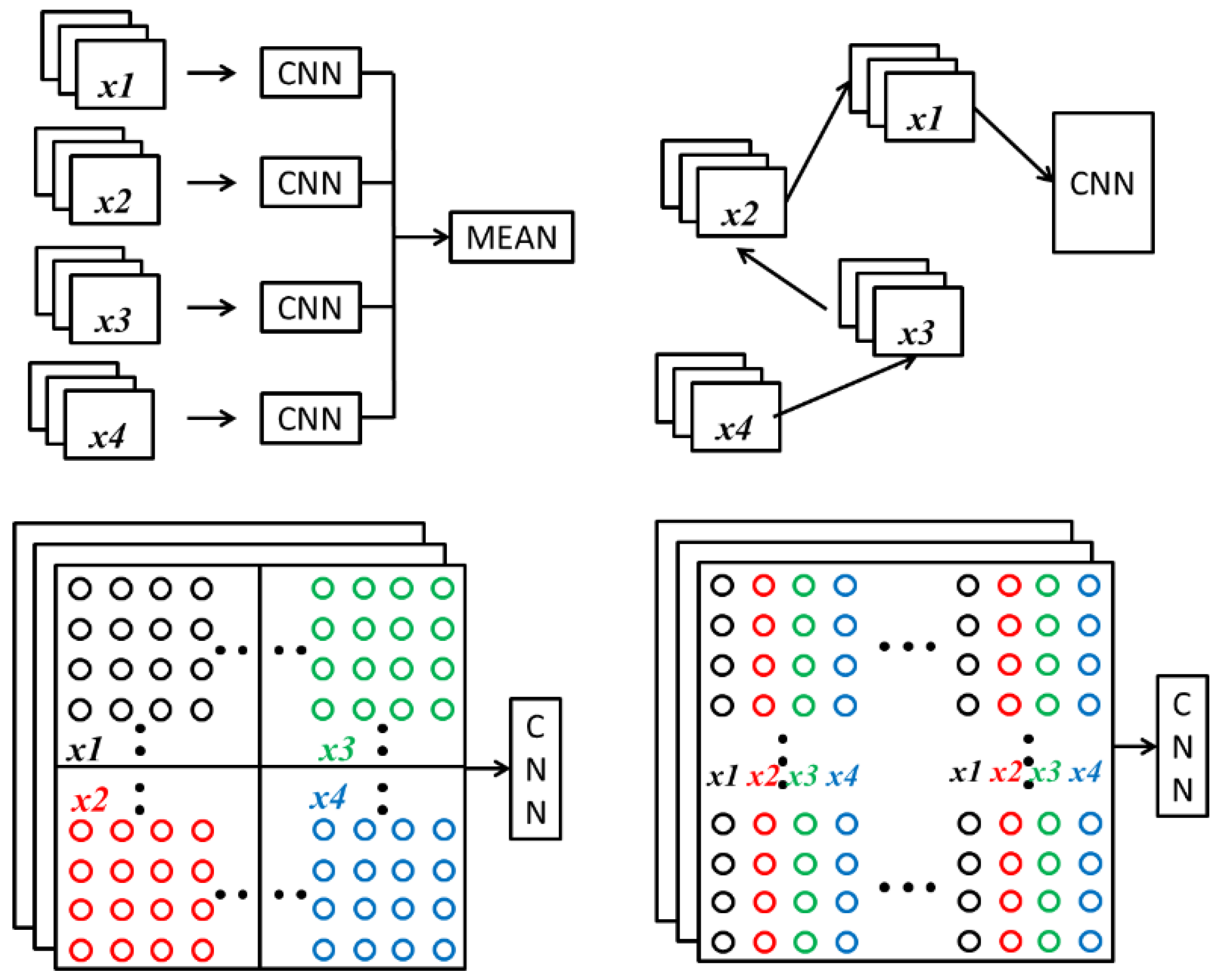
The data used in the CNN include four sequential inputs and one output. Four parameters (hydraulic pressure, hydraulic flow, motor speed and motor torque) from the hydraulic system are taken as the inputs of the CNN and the power generation is the output of the network. Here, the total 100,352 samples acquired from February to April 2017 are sequentially separated into 80,281 as the training dataset (80%), 5019 as the validation dataset (5%) and 15,052 as the test dataset (15%). Firstly, the four time series inputs should be rearranged to a 2D image before applying CNN for regression and prediction. Four different conversion methods are attempted to achieve a better training accuracy, including: (a) results averaged by the individual CNN of the four inputs; (b) four inputs sequentially rearranged before training; (c) a single 2D image being divided into four sub-images formed by four inputs respectively; (d) an image rearranged by four inputs in sequence, as shown in Figure 8.
4.2. Results
This section introduces the results of evaluation of the wave power generation prediction model. Different proposed patterns converted from inputs by various methods are compared firstly. Different input image sizes (28 × 28, 20 × 20, 14 × 14, 10 × 10 pixels) are deployed to discuss how image size could affect the forecasting results. Curve fitting plots from each conversion method are presented for the sake of revealing fitting details. In order to demonstrate the superiority of the methods, the CNN model is employed along with different mainstream supervised modelling approaches, such as ANN, SVM, linear Regression (LR) and regression tree (RT). Finally, the RMSE, MAE and R2 are used as the metrics to evaluate the prediction performance from multiple criteria perspectives.
For both conversion methods and image sizes, as can be seen in Table 2, the proposed networks provide various results in terms of the predicting accuracy. From RMSE and MAE, the 3rd and 4th methods demonstrate the much lower values compared with the 1st and 2nd methods, implying mean lower residuals and higher accuracy are achieved. All three metrics show that the larger the image size and the better performance, and a considerable improvement is made by the 4th method (28 × 28), with the best R2 of 0.96 value being achieved. Results also show that a larger image contains more information compared with an input image of medium and small size, no matter which conversion method is used. In addition, the 3rd and 4th conversion methods obtain lower RMSE and MAE values and a higher R2 value. The forecast from the 2nd method represents the poorest fit with these raw data.
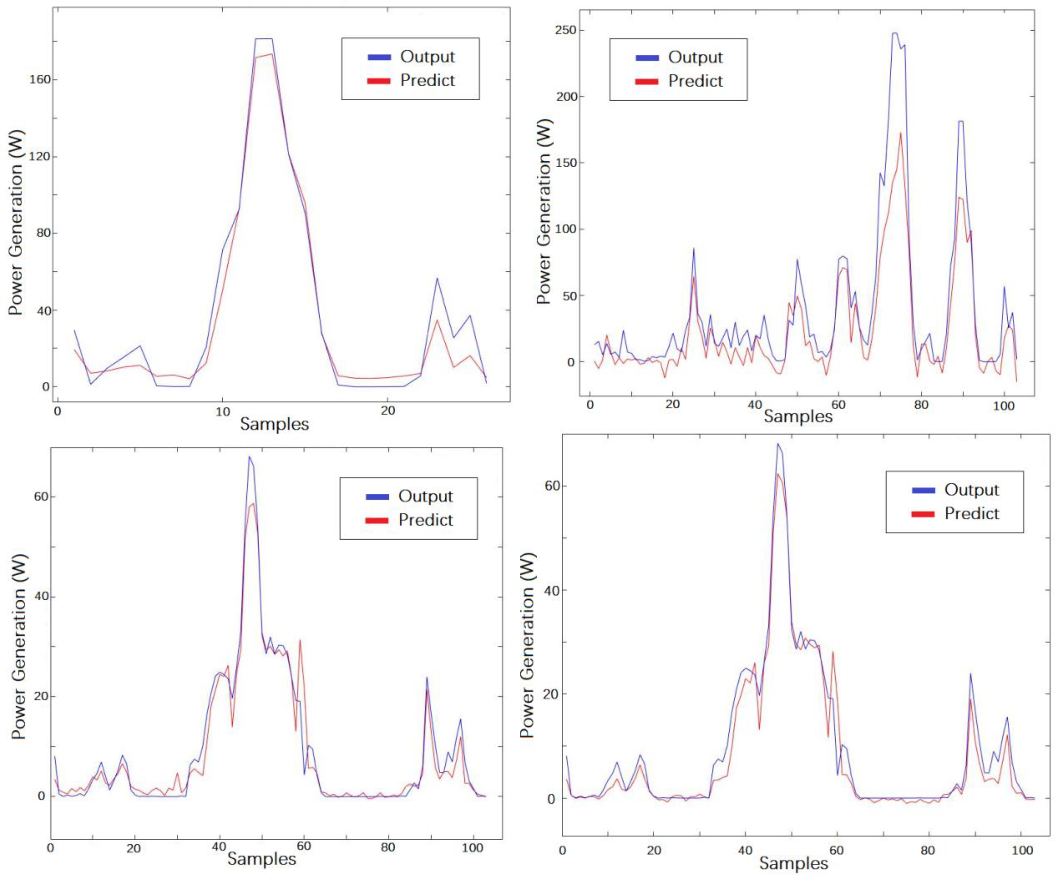
The four plots shown in Figure 9 demonstrate the result as well. The predicted curves fit the real output well in all four plots, except for the top right one that represents the 2nd conversion method. In the top left subplot, the two curves fit much better at the high power level than the low level. The bottom subplots both show remarkable fitting results when forecasting these distinctive fluctuations. The results also illustrate that similar characteristics are extracted from images created by the different data arrange algorithms. Clearly, the top right subplot obtained with the 2nd conversion method, i.e., four inputs applied to the model respectively, exhibits poor fitting in both high and low power levels.
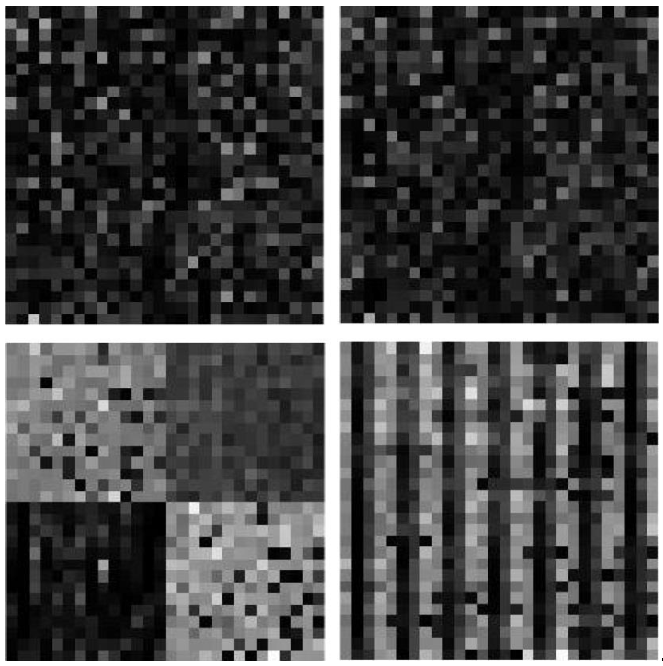
Figure 10 illustrates 2D images of the network input converted from time series 1D inputs. The converted image corresponds to a grey-scale image and every pixel represents the amount of brightness of light [45]. Obviously, the bottom images contain much more features, as can be seen from lines and part of rectangles, which can be recognized by the multi-input CNN model. In contrast, we cannot extract much information from the top images because the features are totally disorganized for the model. This phenomenon explains why different arrangement of pixels in the input image can lead to quite different results, and the more features captured from the inputs, the better results provided from network.
4.3. Discussions
In terms of validation and accuracy, different supervised modelling approaches are applied for comparison, and the results are shown in Table 3. This work was implemented based on a Xeon E3-1271 CPU workstation operating at 3.6 GHz and equipped with 16 GB RAM (Lancaster University, Lancaster, UK) . The training time for the multi-input Convolutional Neural Network (MCNN) was compared with that taken for ML algorithms mentioned above. The SVM takes on an average of 583 s, which means the longest time among them. The CNN algorithm trains no more than 43 s if using the hyper-parameters in Table 1. The MT and BT got an average of 7.21 s and 11.26 s respectively, almost four times faster than the CNN. This indicates that the CNN model provides much higher accuracy even a little longer time consumed than the ML algorithms.
Table 3 also provides sufficient evidence that CNN made considerable achievement in wave power prediction among these ML algorithms. The indicators of the difference between actual and forecast values become quite small if the CNN model is used. SVM and Robust Linear Regression (RLR) produce the worst performance as the MAE value is much higher (more than twice the others) among the five models, which mean these performance measures are much bigger and forecast errors may be easily expected. The R2 values of ANN, medium tree (MT) and boosted tree (BT) show general fitting results. It is worth mentioning that the training of ANN and CNN take a little longer time (more than 43 s in this situation) and the time greatly depends on hidden layers, epochs and break time of the network.
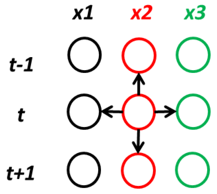
It is known that the form of data modelled in CNN is widely applied in 2D images, which include connection from the neighbourhood [46]. The more features captured from the training images, the better the performance provided by the model. The four image patterns (data arrangements) trained in the different CNN models show distinctive features contained in their images. The large size images contain more features than the small size ones. The prediction is affected by not only the current inputs, but also the connections in the same input series and the adjacent input series in between. In other words, the current inputs combined with adjacent pixels could provide more information than a single input. Let’s take the 4th conversion method as an example, in time t, the is affected by , and , , as shown in Figure 11.
In addition, the number of the convolution layers and feature extractor layers also need to be discussed. Intuitively it would seem that increasing the number of feature maps and convolution layers would improve the accuracy of the model, but actually it works under many conditions. We attempted to increase the number of the convolution layer and pooling layer from 1 to 3 and the feature map from 10 to 100. The neurons for the fully connected layer were also increased from 10 to 100, and the number of layers increased from 1 to 3. Eventually, the training model consumed much more time, though the anticipated results did not appear to be much improved compared with the initial architecture. Consequently, we consider the architecture used in this article is superior enough for training and predicting such a complex problem.
Furthermore, the residual between actual and practical values is supposed to be a function of the inputs. The result is able to perform an early warning to indicate the possible appearance of the anomalies if the residual exceeds a predefined threshold. Thus, this MCNN model could perform condition monitoring and fault diagnosis for the ocean energy systems.
5. Conclusions
In this paper, the power characteristics of a double-buoy oscillating body WEC are presented by analysing open sea testing data. The wave-power curve and the efficiencies of the hydraulic system are investigated to elaborate the connection between wave height and instantaneous power output of the WEC. A Convolutional Neural Network with multiple inputs has been developed for predicting the power output of the near-shore WEC. It uses four hydraulic system parameters as inputs, i.e., hydraulic pressure, hydraulic flow, motor speed and motor torque, and the power output as output. The proposed CNN applies 1D to 2D data conversion to convert time series data into image data.
This result shows that the MCNN provides much better prediction results compared with other mainstream supervised modelling approaches, such as ANN, SVM, LR and RT, with the highest R2 value achieved being 0.96. It can also be found that both the image size and the conversion method can affect the results. The intersectional methods for data conversion with a larger dataset size can capture more features from the training images, thus providing a better model fitting performance. The proposed MCNN is therefore feasible enough for training and predicting the power output from a complex system such as the WEC studied in this paper based on the experimental data.
Besides the time-domain analysis, time-frequency analysis using wavelet transform has also been attempted based on the same data [47,48], the results were found to be widely divergent, and further work will be performed in the near future. Nevertheless, this work makes progress on managing the power generation, transformation and storage of a WEC system for ocean renewable energy systems.
Author Contributions
Conceptualization, C.N. and X.M.; Methodology, C.N. and X.M.; Software, C.N. and X.M.; Formal Analysis, C.N.; Investigation, C.N.; Resources, C.N.; Data Curation, C.N.; Writing-Original Draft Preparation, C.N.; Writing-Review & Editing, C.N. and X.M.; Visualization, C.N. and X.M.; Supervision, X.M.; Project Administration, C.N. and X.M.; Funding Acquisition, C.N. and X.M. conceived and designed the experiments; C.N. performed the experiments and analyzed the data.
Funding
This work received support from CSC (Chinese Scholarship Council) and SFMRE (Special Funds for Marine Renewable Energy) from SOA (Grant number GHME2017ZC01).
Acknowledgments
This research is supported by CSC (Chinese Scholarship Council) and the Engineering Department at Lancaster University, UK. Some of the work received support from SFMRE (Special Funds for Marine Renewable Energy) from SOA (Grant number GHME2017ZC01).
Conflicts of Interest
The authors declare no conflicts of interest.
Abbreviations
| WEC | wave energy converter |
| OBD | oscillating body device |
| CNN | Convolutional Neural Network |
| MCNN | Multi-input Convolutional Neural Network |
| TRL | technology readiness level |
| OWC | oscillating water column |
| PTO | power take-off |
| SCADA | supervisory control and data acquisition |
| ML | machine learning |
| ECMWF | European Centre for Medium-Range Weather Forecast |
| GDAS | Global Data Assimilation Scheme |
| ANN | artificial neural network |
| PV | photovoltaic |
| LS | least-square |
| SVM | support vector machine |
| NN | neural network |
| LSTM | long short term memory |
| DBN | Deep Brief Net |
| RNN | recurrent neural network |
| 1D | 1-dimension |
| 2D | 2-dimension |
| AM | autoregressive models |
| LDS | Linear Dynamical Systems |
| HMM | Hidden Markov Model |
| ReLU | Rectified Linear Unit |
| BP | back propagation |
| SGD | stochastic gradient descent |
| RMSE | root mean square error |
| MAE | mean absolute error |
| R2 | coefficient of determination |
| LR | Linear Regression |
| RT | regression tree |
| RLR | Robust Linear Regression |
| MT | medium tree |
| BT | boosted tree |
References
- Saadat, Y.; Fernandez, N.; Samimi, A.; Alam, M.R.; Shakeri, M.; Ghorbani, R. Investigating of helmholtz wave energy converter. Renew. Energy 2016, 87, 67–76. [Google Scholar] [CrossRef]
- Zou, S.; Abdelkhalik, O.; Robinett, R.; Bacelli, G.; Wilson, D. Optimal control of wave energy converters. Renew. Energy 2017, 103, 217–225. [Google Scholar] [CrossRef]
- Santhosh, N.; Baskaran, V.; Amarkarthik, A. A review on front end conversion in ocean wave energy Converters. Front. Energy 2015, 9, 297–310. [Google Scholar] [CrossRef]
- Magagna, D.; Monfardini, R.; Uihlein, A. JRC Ocean Energy Status Report 2016 Edition; Publications Office of the European Union: Luxembourg, 2016. [Google Scholar]
- Hsieh, M.-F.; Lin, I.-H.; Dorrell, D.; Hsieh, M.-J.; Lin, C.-C. Development of a wave energy converter using a two chamber oscillating water column. IEEE Trans. Sustain. Energy 2012, 3, 482–497. [Google Scholar] [CrossRef]
- Sproul, A.; Weise, N. Analysis of a wave front parallel WEC prototype. IEEE Trans. Sustain. Energy 2015, 6, 1183–1189. [Google Scholar] [CrossRef]
- Contestabile, P.; Iuppa, C.; Di Lauro, E.; Cavallaro, L.; Andersen, T.L.; Vicinanza, D. Wave loadings acting on innovative rubble mound breakwater for overtopping wave energy conversion. Coast. Eng. 2017, 122, 60–74. [Google Scholar] [CrossRef]
- Buccino, M.; Vicinanza, D.; Salerno, D.; Banfi, D.; Calabrese, M. Nature and magnitude of wave loadings at seawave slot-cone generators. Ocean Eng. 2015, 95, 34–58. [Google Scholar] [CrossRef]
- Antonio, F.D.O. Wave energy utilization: A review of the technologies. Renew. Sustain. Energy Rev. 2010, 14, 899–918. [Google Scholar]
- Zhang, W.; Ma, X. Simultaneous fault detection and sensor selection for condition monitoring of wind turbines. Energies 2016, 9, 280. [Google Scholar] [CrossRef] [Green Version]
- Kara, F. Time domain prediction of power absorption from ocean waves with wave energy converter arrays. Renew. Energy 2016, 92, 30–46. [Google Scholar] [CrossRef]
- Reikard, G.; Pinson, P.; Bidlot, J.-R. Forecasting ocean wave energy: The ECMWF wave model and time series methods. Ocean Eng. 2011, 38, 1089–1099. [Google Scholar] [CrossRef]
- Reikard, G. Integrating wave energy into the power grid: Simulation and forecasting. Ocean Eng. 2013, 73, 168–178. [Google Scholar] [CrossRef]
- Uihlein, A.; Magagna, D. Wave and tidal current energy—A review of the current state of research beyond technology. Renew. Sustain. Energy Rev. 2016, 58, 1070–1081. [Google Scholar] [CrossRef]
- Malmberg, A.; Holst, U.; Holst, J. Forecasting near-surface ocean winds with Kalman filter techniques. Ocean Eng. 2005, 32, 273–291. [Google Scholar] [CrossRef]
- Izgi, E.; Oztopal, A.; Yerli, B.; Kaymak, M.K.; Şahin, A.D. Short–mid-term solar power prediction by using artificial neural networks. Sol. Energy 2012, 86, 725–733. [Google Scholar] [CrossRef]
- Zeng, J.; Qiao, W. Short-term solar power prediction using a support vector machine. Renew. Energy 2013, 52, 118–127. [Google Scholar] [CrossRef]
- Peres, D.J.; Iuppa, C.; Cavallaro, L.; Cancelliere, A.; Foti, E. Significant wave height record extension by neural networks and reanalysis wind data. Ocean Model. 2015, 94, 128–140. [Google Scholar] [CrossRef]
- James, S.C.; Zhang, Y.; O'Donncha, F. A machine learning framework to forecast wave conditions. Coast. Eng. 2018, 137, 1–10. [Google Scholar] [CrossRef] [Green Version]
- Vargas, L.; Paredes, G.; Bustos, G. Data mining techniques for very short term prediction of wind power. In Proceedings of the IREP Symposium-Bulk Power System Dynamics and Control-VIII, Rio de Janeiro, Brazil, 1–6 August 2010; pp. 1–7. [Google Scholar]
- Colak, I.; Sagiroglu, S.; Yesilbudak, M. Data mining and wind power prediction: A literature review. Renew. Energy 2012, 46, 241–247. [Google Scholar] [CrossRef]
- Makarynskyy, O.; Makarynska, D.; Rusu, E.; Gavrilov, A. Filling gaps in wave records with artificial neural networks. Marit. Transp. Exploit. Ocean Coast. Resour. 2005, 2, 1085–1091. [Google Scholar]
- Ciortan, S.; Rusu, E. Prediction of the wave power in the Black Sea based on wind speed using artificial neural networks. In Proceedings of the International Conference on Advances in Clean Energy Research (ICACER), Barcelona, Spain, 6–8 April 2018. [Google Scholar]
- Torres, J.M.; Aguilar, R.M.; niga-Meneses, K.V.Z. Deep learning to predict the generation of a wind farm. J. Renew. Sustain. Energy 2018, 10, 013305. [Google Scholar] [CrossRef]
- Liu, H.; Mi, X.; Li, Y. Wind speed forecasting method based on deep learning strategy using empirical wavelet transform, long short term memory neural network and elman neural network. Energy Convers. Manag. 2018, 156, 498–514. [Google Scholar] [CrossRef]
- Shi, H.; Xu, M.; Ma, Q.; Zhang, C. A whole system assessment of novel deep learning approach on short-term load forecasting. In Proceedings of the 9th International Conference on Applied Energy (ICAE), Cardiff, UK, 21–24 August 2017; Available online: https://en.wikipedia.org/wiki/Expected_value#cite_note-Ross-1 (accessed on 21 February 2018).
- Yi, Z. Wind and Wave Analysis of QingShui Bay Based on WRF and SWAN Model. Available online: http://www.docin.com/p-1440602358.html (accessed on 26 April 2018).
- Contestabile, P.; Lauro, E.D.; Galli, P.; Corselli, C.; Vicinanza, D. Offshore wind and wave energy assessment around Malè and Magoodhoo island (Maldives). Sustainability 2017, 9, 613. [Google Scholar] [CrossRef]
- Contestabile, P.; Ferrante, V.; Vicinanza, D. Wave energy resource along the coast of Santa Catarina (Brazil). Energies 2015, 8, 14219–14243. [Google Scholar] [CrossRef]
- Wang, J.; Ma, Y.; Zhang, L.; Gao, R.X.; Wu, D. Deep learning for smart manufacturing: Methods and applications. J. Manuf. Syst. 2018. [Google Scholar] [CrossRef]
- Kempener, R.; Neumann, F. Wave Energy Technology Brief. International Renewable Energy Agency, 2014. Available online: http://www.irena.org/-/media/Files/IRENA/Agency/Publication/2014/Wave-Energy_V4_web.pdf (accessed on 29 June 2018).
- Zang, Z.; Zhang, Q.; Qi, Y.; Fu, X. Hydrodynamic responses and efficiency analyses of a heaving-buoy wave energy converter with PTO damping in regular and irregular waves. Renew. Energy 2018, 116, 527–542. [Google Scholar] [CrossRef]
- Taylor, G.W. Composable, Distributed-State Models for High-Dimensional Time Series. Ph.D. Thesis, Department of Computer Science, University of Toronto, Toronto, ON, Canada, 2009. [Google Scholar]
- Guo, Y.; Liu, Y.; Oerlemans, A.; Lao, S.; Wu, S.; Lew, M.S. Deep learning for visual understanding: A review. Neurocomputing 2016, 187, 27–48. [Google Scholar] [CrossRef]
- Graves, A. Supervised Sequence Labelling; Springer: Berlin, Heidelberg, 2012; pp. 5–13. Available online: http://link.springer.com/10.1007/978-3-642-24797-2_2 (accessed on 5 April 2018).
- Mozo, A.; Ordozgoiti, B.; GoÂmez-Canaval, S. Forecasting short-term data center network traffic load with convolutional neural networks. PLoS ONE 2018, 13, e0191939. [Google Scholar] [CrossRef] [PubMed]
- Shimobaba, T.; Kakue, T.; Ito, T. Convolutional Neural Network-Based Regression for Depth Prediction in Digital Holography. Available online: https://arxiv.org/abs/1802.00664 (accessed on 2 February 2018).
- Suryani, D.; Doetsch, P.; Ney, H. On the Benefits of Convolutional Neural Network Combinations in Offline Handwriting Recognition. Available online: https://www-i6.informatik.rwth-aachen.de/publications/download/1021/Suryani-ICFHR-2016.pdf (accessed on 29 June 2018).
- Wikipedia. Convolutional Neural Network. Available online: https://en.wikipedia.org/wiki/Convolutional_neural_network#Distinguishing_features (accessed on 29 June 2018).
- What are the Advantages of ReLU over Sigmoid Function in Deep Neural Networks. Stackexchange. Available online: https://stats.stackexchange.com/questions/126238/what-are-the-advantages-of-relu-over-sigmoid-function-in-deep-neural-networks (accessed on 29 June 2018).
- Wang, H.Z.; Li, G.Q.; Wang, G.B. Deep learning based ensemble approach for probabilistic wind power forecasting. Appl. Energy 2017, 188, 56–70. [Google Scholar] [CrossRef]
- Zhao, K.; Wang, C. Sales Forecast in E-commerce using Convolutional Neural Network. Available online: https://arxiv.org/abs/1708.07946 (accessed on 29 June 2018).
- Cross, P.; Ma, X. Nonlinear system identification for model-based condition monitoring of wind turbines. Renew. Energy 2014, 71, 166–175. [Google Scholar] [CrossRef] [Green Version]
- Brian, D.R.; Hjort, N.L. Pattern Recognition and Neural Networks, 1st ed.; Cambridge University Press: Cambridge, UK, 2008. [Google Scholar]
- Johnson, S. Stephen Johnson on Digital Photography; O’Reilly: California, CA, USA, 2006; ISBN 0-596-52370-X. [Google Scholar]
- Zhu, A.; Li, X.; Mo, Z.; Wu, H. Wind power prediction based on a convolutional neural network. In Proceedings of the 2017 International Conference on Circuits, Devices and Systems, Chengdu, China, 5–8 September 2017. [Google Scholar]
- Fujieda, S.; Takayama, K.; Hachisuka, T. Wavelet Convolutional Neural Networks for Texture Classification; Cornel University Libruary: New York, NY, USA, 2017. [Google Scholar]
- Polikar, R. The Wavelet Tutorial Second Edition Part I. Available online: http://web.iitd.ac.in/~sumeet/WaveletTutorial.pdf (accessed on 29 June 2018).
Figure 1.
Schematic diagram of the wave power generation system.

Figure 2.
Schematic diagram of the hydraulic oscillating body system.

Figure 3.
Examples of pre-processed data measured from the WEC.

Figure 4.
Comparison of the input and output power of the hydraulic system.

Figure 5.
The comparison of different conversion efficiencies from the hydraulic system, electrical generator and electricity storage.
Figure 5.
The comparison of different conversion efficiencies from the hydraulic system, electrical generator and electricity storage.

Figure 6.
The wave height–hydraulic conversion efficiency curve of this WEC.

Figure 7.
The fundamental structure of the CNN.

Figure 8.
Dataset conversion methods, top left: Four inputs applied to the model respectively, top right: Four inputs applied to the model sequentially, the bottom ones: Four inputs rearranged to the image respectively and sequentially.
Figure 8.
Dataset conversion methods, top left: Four inputs applied to the model respectively, top right: Four inputs applied to the model sequentially, the bottom ones: Four inputs rearranged to the image respectively and sequentially.

Figure 9.
The comparison of the prediction results from different conversion methods based on 28 × 28 dimension image, with 1st to 4th conversion method being presented from top left to right bottom subplot.
Figure 9.
The comparison of the prediction results from different conversion methods based on 28 × 28 dimension image, with 1st to 4th conversion method being presented from top left to right bottom subplot.

Figure 10.
The example of 2D images converted from the 1D inputs.

Figure 11.
The principle of how pixels are affected by adjacent pixels.


Table 1.
List of the values of hyper-parameters used in this network.
| Hyper-Parameters | Values |
|---|---|
| Input variables | 4 |
| CNN Layers | 25 |
| Fully Connected Layer | 40 |
| Predict Layer | 1 |
| Batch size | 20 |
| Number of Epochs | 100 |
Table 2.
Prediction performance of the CNN model through different image sizes and methods.
| Image Size | 1st Conversion Method | 2nd Conversion Method | 3rd Conversion Method | 4th Conversion Method | ||||||||
|---|---|---|---|---|---|---|---|---|---|---|---|---|
| RMSE | MAE | R2 | RMSE | MAE | R2 | RMSE | MAE | R2 | RMSE | MAE | R2 | |
| 28 × 28 | 10.02 | 8.05 | 0.95 | 23.48 | 21.19 | 0.85 | 3.37 | 2.23 | 0.94 | 3.11 | 1.92 | 0.96 |
| 20 × 20 | 16.43 | 8.64 | 0.91 | 29.46 | 23.67 | 0.77 | 3.63 | 1.84 | 0.94 | 3.76 | 2.14 | 0.93 |
| 12 × 12 | 20.48 | 9.63 | 0.87 | 25.21 | 19.82 | 0.83 | 4.45 | 2.81 | 0.91 | 4.25 | 2.45 | 0.92 |
Table 3.
The performance of CNN compared with different supervised modelling approaches (28 × 28 dimension size).
Table 3.
The performance of CNN compared with different supervised modelling approaches (28 × 28 dimension size).
| Approaches | RMSE | MAE | R2 | Time (s) |
|---|---|---|---|---|
| ANN | 2144.83 | 11.38 | 0.83 | 39.19 |
| SVM | 34.88 | 27.10 | 0.69 | 583 |
| RLR | 35.15 | 27.30 | 0.69 | 4.68 |
| MT | 23.36 | 12.92 | 0.86 | 7.21 |
| BT | 20.83 | 12.49 | 0.89 | 11.26 |
| CNN | 3.11 | 1.92 | 0.96 | 42.85 |
© 2018 by the authors. Licensee MDPI, Basel, Switzerland. This article is an open access article distributed under the terms and conditions of the Creative Commons Attribution (CC BY) license (http://creativecommons.org/licenses/by/4.0/).
Share and Cite
MDPI and ACS Style
Ni, C.; Ma, X. Prediction of Wave Power Generation Using a Convolutional Neural Network with Multiple Inputs. Energies 2018, 11, 2097. https://doi.org/10.3390/en11082097
AMA Style
Ni C, Ma X. Prediction of Wave Power Generation Using a Convolutional Neural Network with Multiple Inputs. Energies. 2018; 11(8):2097. https://doi.org/10.3390/en11082097
Chicago/Turabian StyleNi, Chenhua, and Xiandong Ma. 2018. "Prediction of Wave Power Generation Using a Convolutional Neural Network with Multiple Inputs" Energies 11, no. 8: 2097. https://doi.org/10.3390/en11082097
Note that from the first issue of 2016, this journal uses article numbers instead of page numbers. See further details here.