Shale Reservoir Drainage Visualized for a Wolfcamp Well (Midland Basin, West Texas, USA)

Harold Vance Department of Petroleum Engineering, Texas A&M University, College Station, TX 77843-3116, USA
*
Author to whom correspondence should be addressed.
Energies 2018, 11(7), 1665; https://doi.org/10.3390/en11071665
Submission received: 7 May 2018
/
Revised: 22 June 2018
/
Accepted: 25 June 2018
/
Published: 26 June 2018
(This article belongs to the Section L: Energy Sources)
Abstract
:Closed-form solution-methods were applied to visualize the flow near hydraulic fractures at high resolution. The results reveal that most fluid moves into the tips of the fractures. Stranded oil may occur between the fractures in stagnant flow zones (dead zones), which remain outside the drainage reach of the hydraulic main fractures, over the economic life of the typical well (30–40 years). Highly conductive micro-cracks would further improve recovery factors. The visualization of flow near hypothetical micro-cracks normal to the main fractures in a Wolfcamp well shows such micro-cracks support the recovery of hydrocarbons from deeper in the matrix, but still leave matrix portions un-drained with the concurrent fracture spacing of 60 ft (~18 m). Our study also suggests that the traditional way of studying reservoir depletion by mainly looking at pressure plots should, for hydraulically fractured shale reservoirs, be complemented with high resolution plots of the drainage pattern based on time integration of the velocity field.
1. Introduction
The shale revolution responsible for North America’s oil and gas renaissance has seen three waves. The first wave was the rapid expansion, between 2005 and 2010, of hydraulically fractured shale gas wells in the Barnett and other gassy shale plays (Haynesville, Fayetteville, Woodford, Eagle Ford, and Marcellus) with major growth currently confined to the Marcellus shale [1]. The second wave was a shift by North-American operators, starting in 2008, from gas to liquid-rich shale plays like the Eagle Ford and the Bakken [2,3]. The third wave has only just begun with the hydraulic fracturing of multi-stage wells now being successfully applied to re-develop thick shale formations in the Permian Basin. Our study focuses on the production performance of a multistage hydraulically fractures well in the Midland Basin, which comprises the eastern part of the Permian Basin.
With oil and gas prices in the epoch 2014–present being significantly lower than when the North American shale bonanza started in the previous decade [4], operators need innovative insights to improve recovery factors to gain more production income without cost increases. Currently, recovery factors are still a fraction of what industry achieved in conventional hydrocarbon reservoirs [5]. Reservoir and completion engineers are challenged to improve recovery factors of hydrocarbon resources in shale formations. Currently, such recovery factors are typically quite low, perhaps 20% in gas-rich shale reservoirs and less than 10% in liquid-rich plays, which compares poorly to those achieved in conventional reservoirs where ultimate recovery factors range between 40% for oil and 80% for gas [5]. The well stimulation process by hydraulic fracture treatment is a key tool to improve the recovery factors of shale gas and liquids.
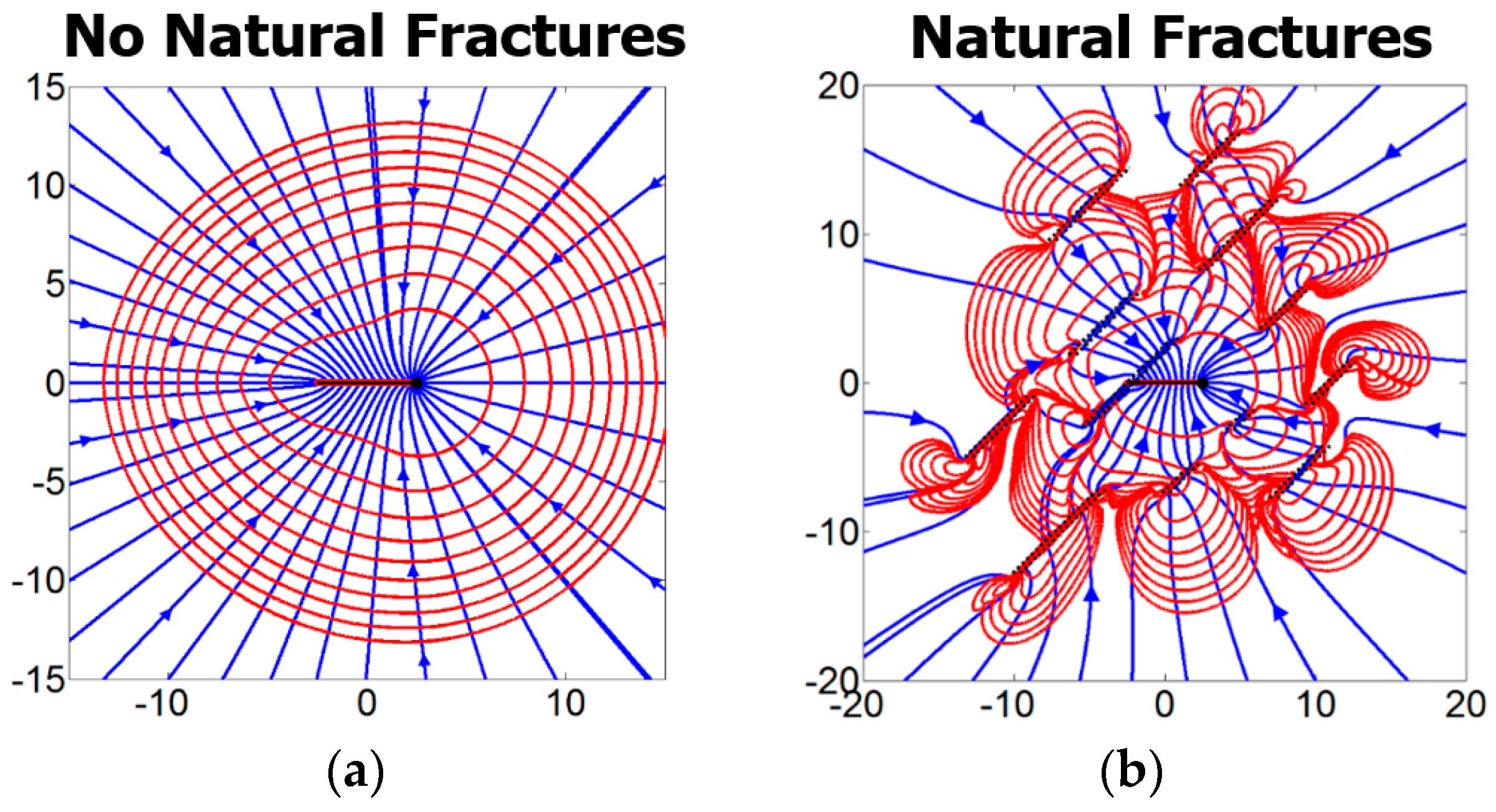
Companies operating the unconventional shale plays, have made advances by adopting a manufacturing model, drilling multiple horizontal wells from a single well pad, completed with 100s of closely spaced hydraulic fractures per well. Next, developing new flow visualization methods to pinpoint where oil moves into the well via the hydraulic fractures has become very important to find ways to further improve the recovery of oil from shale. We developed a grid-less and meshless model tool based on Complex Analysis Methods (CAM), which allows rapid visualization of flow attributes around individual hydraulic fractures, using: (1) pressure field contour plots, (2) velocity field contour plots, (3) streamlines, and (4) drainage contours. The accuracy of the CAM tool has been benchmarked against independent reservoir simulators, which showed no discernable difference in results [6,7,8], except for the higher resolution of the CAM results. The method is suitable for modeling the drainage pattern near multiple hydraulic fractures and natural fractures. Figure 1a,b show an example of how natural fractures can completely redistribute the flow in a reservoir, dependent on the fracture characteristics [9].
Our present study highlights two new insights. The first new insight is that using pressure plots as a proxy for reservoir depletion zones can be misleading. Pressure plots traditionally used to show the depletion of hydrocarbon reservoirs generally suggest that large areas are drained by hydraulically fractured wells [10,11,12]. Our present study shows that velocity plots and drained area plots reveal much more detail about the hydrocarbon migration in shale reservoirs than pressure plots alone. Although pressure plots and the associated velocity field, which is linear to the pressure gradient, are controlled by the same reservoir parameters, velocity front tracking allows the construction of drainage contours, based on the time-of-flight concept, around the stimulation zone. Flow velocities change rapidly with spatial changes in the pressure gradients that drive the fluid flow and only a fraction of the moving fluid reaches the well, due to very slow flow in ultra-low permeability reservoirs (see velocity quantification later in this study).
The second new insight is that micro-cracks may affect the flow field and drain fluid from the matrix deeper than when such cracks would not exist. However, fracture diagnostics precludes the confirmation of the existence of such cracks. Due to the lack of high-resolution fracture diagnostics [13], the extent of the fracture network often is incompletely disclosed and the fracture conductivity of known fractures remains shrouded in uncertainty. Our flow visualization method can show both the matrix drainage by the main fractures and any deeper reach into the matrix when micro-cracks occur as offshoots from the main fractures. This study documents our results and the methodology used is succinctly outlined.
2. Prior Work
Traditionally, the visualization of the fluid migration into the hydraulic fractures of shale reservoirs makes use of general purpose reservoir simulators, primarily developed to model heterogeneities in conventional reservoirs represented by spatial changes in porosity and permeability. Such grid-based solution methods have been modified to account for flow through matrix and fractures of hydraulically fractured wells [14]. Extremely narrow grid sizing is required near fractures to resolve the flow, which makes finite-element solutions time-consuming and costly to produce. A brief review of common methods for modeling flow in hydraulically fractured reservoirs is given below.
2.1. Dual Porosity Models and Limitations
Modeling flow in fractured porous media, such as rocks and unconsolidated sands, are among the most challenging problems both in hydrogeology [15,16] and in reservoir engineering [17,18]. One approach prevalent in simulations of fractured reservoirs uses the dual-porosity model [19,20] and its numerous expansions, which consider a description for a continuously fractured (pseudo-fractured) reservoir, as opposed to descriptions of discretely fractured reservoirs. The reservoir is modeled by separating domains of connected fractures with 100% porosity and a certain assumed permeability with matrix pores acting as storage space. The flow from the matrix to the wellbore is clearly affected by the presence of fractures, which the dual-porosity model attempts to capture by a transfer function using a shape factor. Among the several shortcomings of the dual porosity model, most importantly is the lack of any explicit parameter accounting for fracture density. Transfer functions and shape factors were introduced to control the exchange of fluid between the matrix and the fractures [21,22,23]. Numerous shape factors have been suggested [24,25,26,27,28] after the early work [19,20]. For example, mass transfer from matrix to wellbore would be 25% more effective using a shape factor for a rhombic fracture system rather than a cubic fracture system [28]. Later shape factors included time-dependency of the pressure transfer function. However, all proposed modifications of the shape factor affect the diffusion equation such that a larger shape factor (in the denominator of Equation (2) in Warren and Root [20]) will result in steeper pressure gradients.
2.2. Discrete Fracture Network Models and Limitations
The benefits of high-resolution modeling of the detailed fracture patterns in shale by numerical methods include [29]: (1) accurate estimation of reserves and recoverable resources, (2) validation of analytical models, and (3) optimization of fracture and completion designs. The effect of natural fractures (positive/negative) on the stimulation of unconventional reservoirs has been well documented [30,31,32]. The introduction of constrained discrete fracture networks (DFN) [33] where a secondary variable was used to control the randomness of the DFN models did not solve multiple problems inherent to a discrete description of the natural fractures. Alfred et al. [34] describe additional issues of a DFN approach, which includes the major issue of upscaling [35] when transferring the fracture information to the continuum world commonly used in reservoir simulation and in our case, in geomechanical modeling. To honor structural geology concepts rather than incomplete statistics, the Continuous Fracture Modeling (CFM) approach was proposed [36,37,38].
Aimene and Nairn [39] and Aimene and Ouenes [40] introduced the Material Point Method (MPM) to facilitate the representation of the natural fractures in a multi-scale continuum problem. MPM combines Lagrangian and Eulerian descriptions of the material and in doing so overcomes the inherent drawbacks of methods relying on using only one perspective. This is achieved by discretizing the material into Lagrangian material points. These material points reside in an Eulerian mesh that is used to solve the equations of motion during a time step. An interpolation from the material points to the mesh nodes allows for this dual perspective to be used. The MPM is an example of a meshless method [41] as the mesh is not required for a full description of the material, it is only used for calculation purposes. The proposed MPM workflow [42,43] reduces uncertainties in fracture design and optimization through the use of half lengths derived from the validated geomechanical strain.
The limitations of local grid refinements (LGR) to capture the pressure field near fractures in DFN are well known. One drawback is that LGR is computational intensive, especially when using structured Cartesian grids [44]. Another shortcoming is that such Cartesian grids cannot effectively represent complex and non-planar fracture networks. The latter can be better captured using unstructured grids to define Voronoi cells [29,45,46]. Some gains in computational time can be achieved using coarse scale parameters from numerical homogenization to upscale the non-transient regions in the reservoir model [47]. However, simulations with gridded and meshed finite elements remain computationally intensive, especially for multi-stage wells, which may have several hundred perforation zones in a single well. Further, reduction of computation time is typically achieved by applying so-called stencils to represent a multiple fractured well system by collocation of repetitive flow cells around a single or a small subset of the hydraulic fractures. The justification of such simplification typically were based on older completion techniques with well spacing of 120 m (394 ft), which reduced the effect of frac interference [29,44]. However, with today’s tight frac spacing reduced to 1/10th (or even 1/20th in 2018 fracture treatments) of the spacing used in the cited studies, frac interference effects occur early in the well-life and preclude the use of stencils. We agree with prior authors [48,49] that representing a multiple-fractured horizontal-well system by repetitive elements of a single fracture is not warranted.
An additional limitation of numerical codes for multi-stage fractured wells with long computation times is that achieving global optimization remains out of reach when multiple realizations of all potential fracture designs and well spacing cannot be computed due to practical time constraints. Numerous attempts exist to improve optimization routines, including, but not limited to, Bayesian optimization [50], parametric sensitivity analysis [51,52], genetic algorithms for derivative-free optimization [53,54], and particle swarms approach [55,56].
2.3. Analytical Models
Early analytical models of flow through rock fractures are mainly limited to cubic law formulations for fluid flow transport through just a single fracture [57], expanded in later work with factors accounting for wall roughness [58,59,60]. The transient effect of stress on flow in a single fracture due to dilation effects has also been quantified [61,62,63], with further efforts to account for inertia effects due to turbulent fluid at high rates of injection [64]. Recent studies account for solute transport [65,66], and chemical interaction [67,68], all confined to a single fracture model.
2.4. Drained Rock Volume
Prior studies have emphasized that the drainage region where reservoir fluid is moving due to the pressure gradient differs from the drained region, defined by the much smaller volume of fluid that has moved into the well after a certain time [69,70]. Closer study reveals the important distinction between stimulated rock volume (SRV) and fluid that actually reaches the well within practical field operation times, which we refer to as the drained rock volume (DRV). Pressure plots alone convey reservoir regions affected by flow, but are inconclusive to establish the DRV. Pressure plots do not reveal directly where fluid is stagnant. Pressure is a scalar quantity and velocity is a vector quantity. The difference is relevant, because the fact that fluid drainage rates are highest near the tips of hydraulic fractures is not quickly seen from pressure plots. Contouring of the velocities reveals that new insight immediately (see Section 4). Additionally, we can use velocities to track the drained volume using time-of-flight contours. The so-called depth of investigation increases as the pressure wave propagates from the well system deeper into the reservoir and closely corresponds to the outline of the SRV [71,72,73]. However, the areal extent of fluid drained may be much smaller than suggested by using pressure plots only. Using pressure depletion plots in combination with velocity field contour plots and time-of-flight based drainage contours, using the transient velocity field vectors to track individual fluid elements, is very useful for hydraulically fractured wells and arguably should be used as a new industry standard.
Exactly how much drainage occurs, and where the fluid produced in fractured wells comes from, can be visualized with our method at a high resolution [8]. Our present approach applies calculus from complex analysis to provide closed-form solutions for single phase flow involving an unlimited number of interacting fractures [9].
3. Methodology
Our modeling approach using CAM, side-steps the drawbacks of LGR and other gridded solutions (outlined in Section 2.2), by using a grid-less and meshless solution strategy, while still being able to model transient flow by time-stepping streamline integrals with very small time intervals to achieve smooth particle paths [74]. Single-phase flow in porous media can be modeled with analytical descriptions as has been advocated in many classical studies (e.g., Muskat [75,76]). The closed-form solution is commonly used to map curvilinear line-integrals to identify streamlines [77,78]. Our novel approach using complex analysis methods has been applied to fluid flooding and sweeping of hydrocarbon reservoirs with finite boundaries [6] and infinite boundaries [79,80]. Investigations of how hydraulic fractures drain the matrix in shale reservoirs are also possible using our method for streamline simulation and fluid time-of-flight tracing based on complex analysis methods. Applications include the visualization of hydrocarbon migration toward hydraulically fractured wells [9], and fluid drainage near multi-fractured horizontal wells with fracture hits [8,74,81]. The key algorithms and key workflow steps used in our model method are explained below.
3.1. Complex Potential and Generic Velocity Potential
The complex potential Ω(z) links the stream function (ψ) and potential function ():
The velocity components (vx and vy) can be obtained using and . The full velocity field V(z) is given by the velocity potential:
The fluid flow is assumed irrotational, incompressible, immiscible and isothermal, such that the viscosity and density of the reservoir fluid remains constant. Capillary pressure, wettability and relative permeability effects are neglected. Details on complex analysis and flow applications can be found elsewhere [82,83,84,85,86,87].
3.2. Single Point Source
The interval source and dipole elements used in our study are based on the superposition of point sources and point sinks. The complex potential centered of a source/sink flow centered at the origin with time-dependent strength m(t), is:
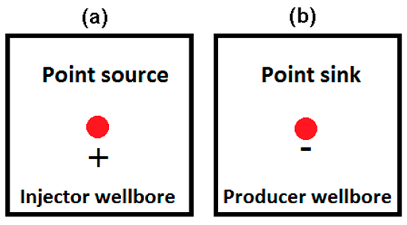
The flow in a porous medium due to a pressure gradient near a vertical injector wellbore in the planar (x,y) field is modeled by a point source (Figure 2a). Likewise, flow toward a vertical producer wellbore is represented by a point sink (Figure 2b). The corresponding velocity field is given by [79,80]:
where m(t) is the well strength (producers m(t) > 0; injectors m(t) < 0) in wells located at zc.
Strength m(t) for a well with productivity q(t) (m3·s−1), reservoir height h (m), and reservoir porosity n is:
Factor B is the volume factor defined by the ratio of any oil volumes under reservoir conditions divided by that oil volume in the stock tank at surface conditions.
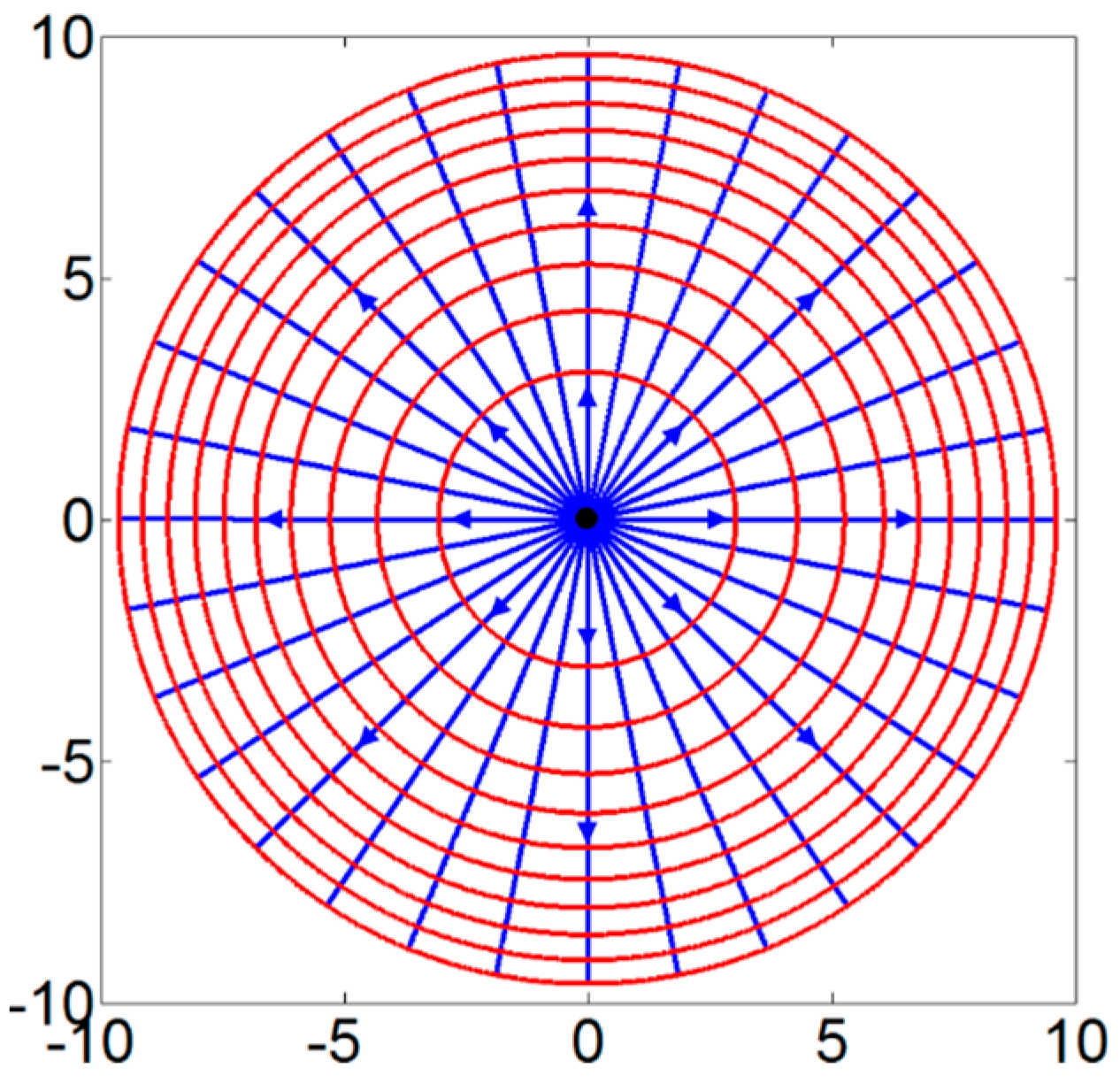
Figure 3 gives streamlines and time-of-flight contours for a homogenous horizontal reservoir due to fluid injection from a single vertical well with constant injection rate. Radial flow results in isochronous time-of-flight contours that are circles.
3.3. Interval Source
The hydraulic fractures in our model were modeled by interval-sources, obtained by superposing an infinite number of point sources (Figure 4). Assuming an interval source centred at the origin, with total length L and strength m(t), the complex potential is [7]:
Rotation of the interval-source by angle β and shifting its centre from the origin to coordinate zc (Figure 5) yields:
The complex potential for N interval-sources, each with their own angle βk, centre zck, length Lk and strength mk, reads [8]:
Differentiation of the above expression with respect to z, results in the velocity field expression for N interval sources with arbitrary orientations [8]:
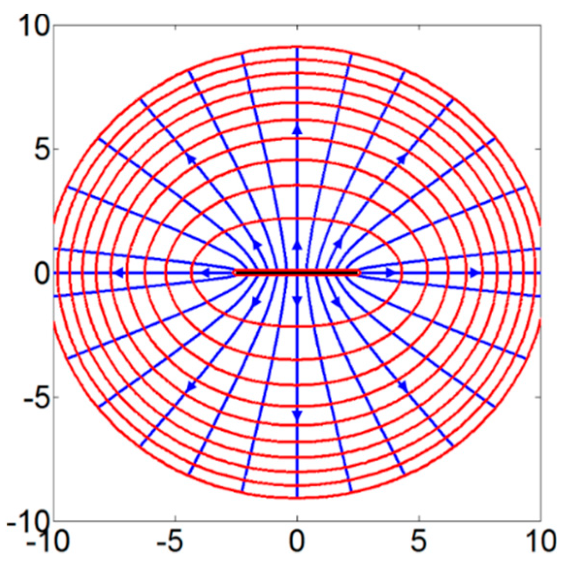
Streamlines and time-of-flight contours for the area drained by a vertical fracture are obtained with our streamline tracing algorithm and visualized in Figure 6. The isochronous time-of-flight contours are confocal ellipses.
3.4. Single Point Dipole
The micro-cracks in our study were modeled by line dipoles. The point dipole, also known as point doublet, singularity doublet and singularity dipole, is a common occurrence in amongst other electromagnetism [88], aerodynamics [89], and fluid mechanics [90]. Deriving the point dipole velocity field entails combining the velocity fields of a point source and point sink (Figure 7) in a limiting process. Placing a point sink and point source of equal but opposing strengths on the real axis at a distance of 2ε from each other, meaning their locations are ε and −ε respectively, yields the velocity field:
The point dipole is then obtained by letting 2ε approach zero while the product q(t)∙2ε remains constant (meaning q(t) increases inversely proportional to distance 2ε). By defining this constant as υ(t) = q(t)∙2ε, we find that the velocity field for the point dipole, located at the origin, is:
Rotating the point dipole of expression (11) counter-clockwise by angle β and placing it at location zk is possible by employing the conformal mapping f(z) = e−βi(z − zk) and evaluating V(f(z))·f’(z). This results in the velocity field formula:
Note that υ is the strength of the point dipole and, as a result of the limiting process, its unit is (m4·s−1). The complex potential of a point dipole is hence given by:
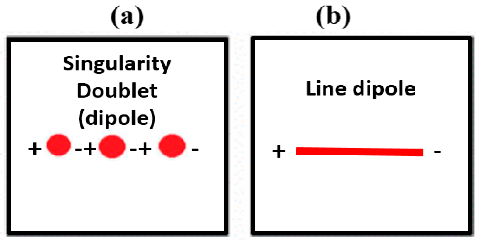
3.5. Line-Dipole
The analytical point dipole in expression (12) has its source side pointing parallel to the real axis, to the right, if β = 0 (Figure 8). We derive a line-dipole, starting with β = 0 and its center at real axis coordinate xc. The resulting velocity field is:
Next combine j of the point dipoles, with a uniform strength υ(t):
To transform this expression into a Riemann integral, the interval [−0.5L, 0.5L] is partitioned into j intervals, by defining the j + 1 points:
Therefore, each point dipole is located at:
In order to turn expression (15) into a Riemann integral, the spacing between two point dipoles (Δxk) needs to be defined:
Multiplying expression (15) with L/L and splitting the sum then gives:
By letting j increase without bound, the last term in expression (19) goes to zero and a Riemann integral is obtained because Δxk goes to zero. The resulting integral and velocity field is:
Rotating this expression and shifting the center is again achieved with the conformal mapping f(z) = e−βi(z − zc) and by evaluating V(f(z))·f′(z). The velocity field for the line-dipole is therefore:
Expression (21) is similar to the one in Weijermars and Van Harmelen [79], though more explicitly formulated. The complex potential of a line-dipole is hence given by:
3.6. History Matching and Flux Allocation
A general expression used for history matching of the prototype well rate is given by Duong [91] (using field units in bbls/day):
Cumulative oil production is:
The next step is to allocate total well production rates to the individual fracs in our drainage model:
C = 5.61458333 converts field input units of in stb/day to field output units of in ft3/day, and WOR = Swater/Soil, the respective saturations of water and oil.
In our study, the total type curve output, qwell(t), was simply prorated to the stages studied (13 out of 33) and divided proportional to the surface area of each frac stage (as determined by the product of frac heights, hk, and lengths Lk) relative to the total surface area of the 13 fracs, and correcting for the water to oil ratio, WOR:
The prorated flux per frac over time was used in the drainage visualization of our study.
3.7. Oil in Place and Recovery Factor
The produced oil can be compared to the original oil in place:
With field units inputs used as follows: 7758 = barrels (bbls) of oil per (acre·ft); A = area in acres (TBD in acres); h = height in feet; n = porosity; Sw = water saturation; B = volume factor.
The oil recovery factor is:
with F = Recovery factor, and Np(t) the cumulative production (stb) till a certain time t.
F(t) = Np(t)/OOIP
3.8. Pressure Field
For a hydrostatic reservoir, the initial reservoir pressure P0 is determined by the hydrostatic pressure gradient times reservoir depth (d):
The hydrostatic pressure gradient typically is . The pressure change due to production or injection is obtained from:
μ is the viscosity (psi·day or Pa·s, or Poise), k is the permeability (ft2 or m2 or Darcy).
The reservoir pressure consequent to the well flow will be:
Each pressure field plot is generated by evaluating the pressure differential Equation (31) for a large number of complex-valued coordinates z, in conjunction with Matlab’s command ‘contourf’.
3.9. Streamline Tracing
The streamline tracing method uses a first order Eulerian displacement scheme. The initial particle position is z0 (in complex coordinates) at time t0 (unit in (s); see Weijermars et al. [7] for a non-dimensional approach). The velocity field V(z,t) needs to be solved to obtain the velocity vector components (vx and vy) for all positions of tracer elements at times t1, denoted by z1(t1):
The term v(z0(t0)) in expression (33) is the velocity of the traced particle at time t0 and location z0, for which the velocity field V(z,t) is used. The size of the time step is Δt. The locations of tracer elements at time tj are:
In Matlab we evaluate expression (34) by using the corresponding velocity field V(z,t) as follows:
In order to maintain smooth streamlines and time-of-flight contours (TOFCs), the time step Δt needs to be smaller when the strength of point sources/sinks increases. The velocity field plots in this study map the spatial variation in the magnitude of the fluid phase velocity, which is obtained by taking the absolute value |V(z,t)| at a given time t. Each velocity magnitude contour plot uses a large number of complex-valued coordinates z, in conjunction with Matlab’s command ‘contourf’.
4. Results
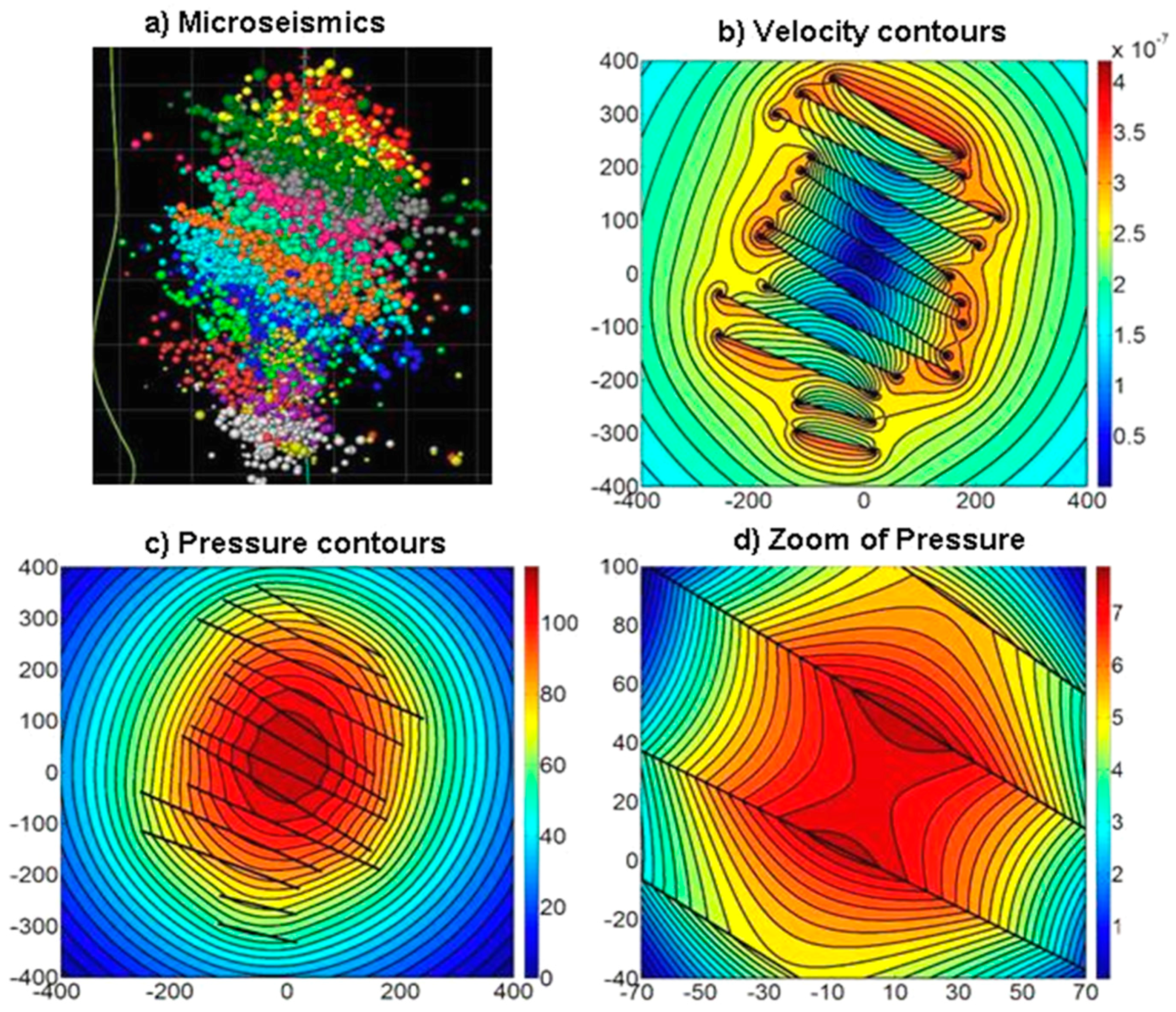
Our flow visualization method can show both the matrix drainage by the main fractures and any deeper reach into the matrix when micro-cracks occur as offshoots from the main fractures. First we show the drainage area when no micro-cracks develop. The locations of the main fractures for each stage of the multi-staged fractures in our prototype well were inferred from the micro-seismic image recorded by the operator during the frack job (Figure 9a). The images of Figure 9b–d show the reservoir response to drainage by a hydraulically fractured, horizontal well after 1 month of production. A summary of input data is given in Table 1. The table includes a description of hydraulic fracture geometry and dimensions, the well productivity based on Duong parameters, original oil in place (OOIP) parameters, and other reservoir parameters.
The velocity plot (Figure 9b) reveals that the oil migrates fastest near the tips of the fractures, with an interior region between the fractures draining much slower. Classical analytical flow models [92] asserted that no fluid flow would occur from matrix into the fracture tips. Only flow of matrix normal to the fracture is assumed, which is clearly not what we see in our CAM simulations where flow near the fracture is fastest and not following sub-parallel or linear streamlines, but more complex particle paths. The simplification of linear flow would lead to overestimation of diffusion to the fracture, particularly when such fractures are short.
4.1. Velocity Field Versus Pressure Plots
The velocity field near hydraulic fractures is rarely visualized in commercial reservoir simulators [93,94]. Pressure depletion plots (Figure 9c) are commonly used as a proxy for drainage of the reservoir. The reservoir pressure when production starts is replaced by an evolving pressure gradient. The steepest pressure gradients occur at the onset of production, with local variations of higher and lower gradients. Figure 9c has the steepest pressure gradients between the red and blue zones (with tighter contour spacing), which broadly coincide with the region of higher flow velocities peripheral to the frac tips (Figure 9b). In commercial simulators, pressure plots resemble the analytical solution of Figure 9c but have limited resolution due to finite grid size and computational time limitations. Our model based on closed-form formulae provides infinite resolution and allows for the computation of a detailed pressure contour map for the central region between the fracs (Figure 9d). Due to relatively shallow pressure gradients, flow in the central zone is slowest. Contoured for smaller changes, pressure gradients still exist in the central region (Figure 9d), but pressure differences are more subtle than elsewhere in the fracked region. The shallow pressure gradient is the reason why the flow is nearly stagnant in the central region between the frac clusters (Figure 9b).
4.2. Implications for Production Efficiency
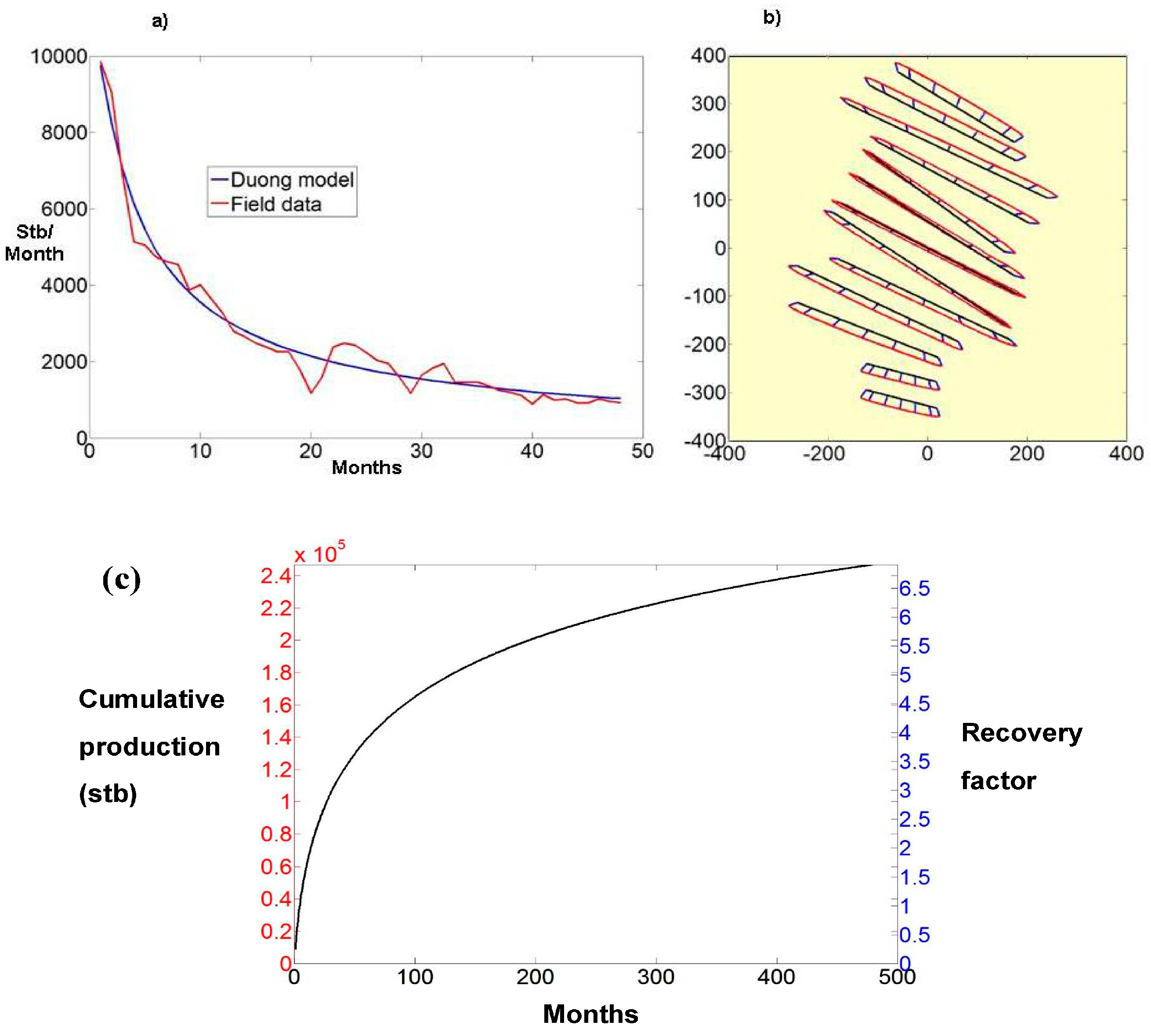
A prototype well that had 50 month historic production data was history matched with a decline curve using a Duong model [81,91,95]. The well type curve for Wolfcamp shale in the Midland Basin, West Texas, is given in Figure 10a. The production forecast was used for production allocation to individual fractures proportionally to each frac stage (see Section 3.6). The width of the drained matrix region around the fractures is visualized using the allocated well flux (Figure 10b). Even after 40 years of production, large portions of the matrix between the fractures remain un-drained. The drainage area and pressure plots were generated using a flow reversal principle: the produced fluid was injected back into the reservoir at the same rate as produced, which allows the construction of time-of-flight contours for the drained rock volume (Figure 10b). All pressure plots show positive pressure, but are equivalent to pressure depletion plots by taking the negative of the pressure scale.
4.3. Recovery Factors
Figure 10b shows the total drainage area for 40 years of production and the narrow region drained corresponds to the cumulative production given by the type curve (Figure 10a). OOIP of the prototype well was estimated for a well spacing of 320 acre/well resulting in a recovery factor of only 6% after 40 years, with 4% recovery already achieved after 5 years. Figure 10c plots the cumulative production and the corresponding recovery factor appreciation over a 40 year field life. These results are based on the history matched and drained rock volume (Figure 10b) obtained by our simulation method. Large undrained (dead) zones occur between the principal fracture zones. However, when micro-cracks are present to drain the deeper matrix, the dead zones may be narrower, which was further investigated.
4.4. Micro-Cracks
The CAM model can be adapted to account for drainage by micro-cracks, were these to occur, that reach deeper into the matrix. Such fractures are currently below the resolution of fracture diagnostics. Unknown matrix micro-cracks acting as hydraulic conduits may drain the matrix further away from the main fractures. Assuming micro-cracks may develop in hydraulically fractured shale reservoirs, the degree of micro-crack contribution to shale drainage will vary with the density and hydraulic conductivity of such cracks.
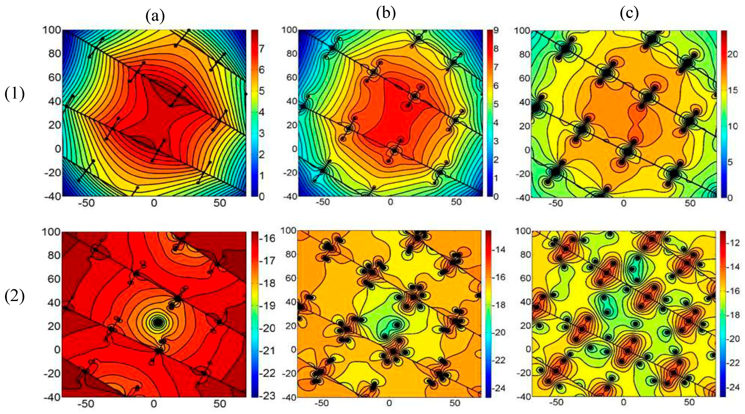
The flow support that hydraulic fractures receive from the microcracks was simulated using line dipoles (see Section 3.5). The strength of dipoles was systematically varied relative to the hydraulic fractures (modeled by interval sources) to show the effect on the drained region in our model. Examples of micro-crack assisted flow in the central region of the multistage fractured well of Figure 9 are shown in Figure 11. What the dipole fracs drain around the micro-crack tips as a consequence of their conductivity being higher than that of the matrix is transported toward the main hydraulic fractures. The depth of the drained area and length of the dipoles representing the micro-cracks is determined by the assigned strength of the dipole relative to that of the interval source used to model the hydraulic fracs. The combined dipole strength of micro-cracks that are connected to a particular hydraulic fracture is variable: equal to the hydraulic fracture strength (Figure 11a), five times the hydraulic fracture strength (Figure 11b), and 10 times the hydraulic fracture strength (Figure 11c).
The pressure plots (Figure 11a–c, row 1) show pressure contours begin to bungle near the micro-cracks when the hydraulic conductivity is larger. Such relatively steep pressure gradients are absent in Figure 9d, which is free of micro-cracks. The flow velocities are clearly enhanced around the micro-cracks (Figure 11a–c, row 2), due to the steep pressure gradients induced near the cracks (Figure 11a–c, row 1). As a result, the micro-cracks would extend the drainage region deeper into the matrix (Figure 11) as compared to situations where micro-cracks are absent (Figure 10b). The velocity peaks are confined to the immediate vicinity of the micro-cracks (Figure 11b,c, row 2), which concur with the locations were pressure gradient are steepest and pressure contours bungle (Figure 11b,c, row 1). The consequent drained region for each case is visualized in Figure 12. The higher resolution images show locally enhanced pressure gradients (Figure 11, row 1) and flow velocity peaks (Figure 11, row 2) occur near the micro-cracks, which facilitate the flow from the deeper matrix regions toward the main fractures.
5. Discussion
Our study suggests that matrix drainage by hydraulic fractures can be accelerated by micro-crack systems. Micro-crack tips drain deeper into the matrix as a consequence of their conductivity being higher than that of the matrix and thus may act as hydraulic fairways. The results show that micro-cracks will improve the drainage depth, but the existence of such micro-cracks is beyond the resolution of current fracture diagnostics. Although our method can visualize flow around the main fractures and any micro-cracks at high resolution, uncertainty remains about the precise location and geometric complexity of the micro-cracks. The relative strengths of dipoles, in our model, may be systematically varied relative to the interval source to show the effect of the micro-crack drainage with different hydraulic conductivity. Darcy’s law diffusion based flow descriptions was used to characterize the drainage of the SRV. This assumption implies nano-scale effects such as osmosis and capillary effects do not invalidate the macroscopic flow description. Future work should account for such nano-scale effects. In any case, micro-cracks would enhance and deepen the matrix area drained by the main hydraulic fractures.
Micro-cracks incorporated in the simulation method are synthetic and hypothetical. Such micro-cracks may contribute to the productivity of the well. However, any net gain in productivity is not accounted for in our model, because the net flux is history matched against the actual production, which fixes the 40 year production curve. What the model shows is that the drained rock volume, in the absence of micro-cracks, remains confined to the immediate vicinity of the hydraulic main fractures. Consequently, we are not underestimating well productivity or recovery factors. The main issue is that the region that will be drained may shift to the interior of the matrix (away from the main fractures) due the presence of micro-cracks.
Several simplifying assumptions are acknowledged. Multiphase flow is not included in our current model, for Wolfcamp B wells, reservoir pressures do not stay above the bubble-point for the lifetime of a well. However, we think the effect on well productivity in the oil window is immaterial due to the low gas content of the wells and late life well productivity contributes little to the cumulative production of the well. Although multiphase flow is not included in our current model, bubble-point effects can certainly be incorporated (subject of new work).
Our conclusion that the highest gradients will occur around the fracture tips, may be nuanced when proppant density varies and premature screen out occurs at fracture tips during the fracture treatment. When the flux around the tip is limited by the connectivity from the tip of the fracture to the wellbore, the flux will shift inward, which is accounted for in a forthcoming paper from our research group [96].
6. Conclusions
We conclude that even when micro-cracks develop minor splays into the matrix, the region between the larger master fractures will remain largely un-drained. The flow velocity and pressure gradients for both the main hydraulic fractures and micro-cracks will be largest near the fracture tips. The smallest velocities and flow stagnation occur in the zones between competing fractures, where the pressure gradients are shallower and become zero in pressure culmination points. The consequent oil entrapment between fractures would not occur in conventional, high-permeability reservoirs, because even slowly moving reservoir fluids would still reach the well on the time scale of the field life (5–50 years). However, unconventional reservoir rocks such as shale with permeabilities in the nano-Darcy range have ultra-low flow rates, even near the fracture tips, in the order of 10−7 m·s−1, the rate at which finger nails grow.
The cluster spacing in the Wolfcamp well studied here is already tight (60 ft). Closer spacing of the fractures would accelerate early production but still creates flow stagnation points between the fractures. However, the un-drained oil occurring between the closely spaced fractures (in low permeability reservoirs with ultra-low flow rates) may be recovered by the refracking of shale wells with perforations placed midway between the prior cluster spacing and fracture initiation points. The second generation of hydraulic fractures will tap into the earlier, stagnant flow regions. The refracs will improve the recovery factors and this may boost well economics accordingly.
Author Contributions
Conceptualization, R.W.; Methodology, R.W.; Software, A.v.H. and R.W.; Validation, R.W. and A.v.H.; Formal Analysis, R.W. and A.v.H.; Investigation, R.W. and A.v.H.; Resources, R.W.; Data Curation, R.W.; Writing-Original Draft Preparation, R.W.; Writing-Review & Editing, R.W.; Visualization, R.W. and A.v.H.; Supervision, R.W.; Project Administration, R.W.; Funding Acquisition, R.W.
Funding
Funds for this study were provided by the Texas A&M Engineering Station (TEES) and the Crisman-Berg Hughes Consortium. Proprietary well data were made available by Pioneer with support of both the Texas Oil and Gas Institute and University Lands.
Conflicts of Interest
The authors declare no conflict of interest.
References
- Weijermars, R. US shale gas production outlook based on well roll-out rate scenarios. Appl. Energy 2014, 124, 283–297. [Google Scholar] [CrossRef]
- Weijermars, R.; Paradis, K.; Belostrino, E.; Feng, F.; Lal, T.; Xie, A.; Villareal, C. Re-appraisal of the Bakken Shale Play: Accounting for Historic and Future Oil Prices and applying Fiscal Rates in North Dakota, Montana and Saskatchewan. Energy Strategy Rev. 2017, 16, 68–95. [Google Scholar] [CrossRef]
- Weijermars, R.; Sorek, N.; Seng, D.; Ayers, W. Eagle Ford Shale Play Economics: U.S. versus Mexico. J. Nat. Gas Sci. Eng. (JNGSE) 2017, 38, 345–372. [Google Scholar] [CrossRef]
- Weijermars, R.; Sun, Z. Regression Analysis of Historic Oil Prices: A Basis for Future Mean Reversion Price Scenarios. Glob. Finance J. 2018, 35, 177–201. [Google Scholar] [CrossRef]
- Task Force. Unconventional Reserves Taskforce—Report to Participating Societies. Final Report—1st March 2016. Available online: https://www.spwla.org/Documents/SPWLA/TEMP/Unconventional%20Taskforce%20Final%20Report.pdf (accessed on 25 June 2018).
- Nelson, R.; Zuo, L.; Weijermars, R.; Crowdy, D. Outer boundary effects in a petroleum reservoir (Quitman field, east Texas): Applying improved analytical methods for modelling and visualization of flood displacement fronts. J. Pet. Sci. Eng. 2017, 166, 1018–1041. [Google Scholar] [CrossRef]
- Weijermars, R.; van Harmelen, A.; Zuo, L. Controlling flood displacement fronts using a parallel analytical streamline simulator. J. Pet. Sci. Eng. 2016, 139, 23–42. [Google Scholar] [CrossRef]
- Weijermars, R.; van Harmelen, A.; Zuo, L.; Nascentes, I.A.; Yu, W. High-Resolution Visualization of Flow Interference between Frac Clusters (Part 1): Model Verification and Basic Cases. In Proceedings of the Unconventional Resources Technology Conference, Austin, TX, USA, 24–26 July 2017. [Google Scholar]
- Van Harmelen, A.; Weijermars, R. Complex analytical solutions for flow in hydraulically fractured hydrocarbon reservoirs with and without natural fractures. Appl. Math. Modell. 2018, 56, 137–157. [Google Scholar] [CrossRef]
- Yu, W.; Wu, K.; Zuo, L.; Tan, X.; Weijermars, R. Physical Models for Inter-Well Interference in Shale Reservoirs: Relative Impacts of Fracture Hits and Matrix Permeability. In Proceedings of the SPE Unconventional Resources Technology Conference, San Antonio, TX, USA, 1–3 August 2016. [Google Scholar] [CrossRef]
- Cipolla, C.L.; Wallace, J. Stimulated Reservoir Volume: A Misapplied Concept? Presented at the SPE Hydraulic Fracturing Technology Conference, The Woodlands, TX, USA, 4–6 February 2014. [Google Scholar]
- Wu, R.; Kresse, O.; Weng, X.; Cohen, C.; Gu, H. Modeling of Interaction of Hydraulic Fractures in Complex Fracture Networks. Presented at the SPE Hydraulic Fracture Technology Conference, The Woodlands, TX, USA, 6–8 February 2012. [Google Scholar]
- Grechka, V.; Li, Z.; Howell, B.; Garcia, H.; Wooltorton, T. High-resolution microseismic imaging. Leading Edge 2017, 36, 822–828. [Google Scholar] [CrossRef]
- Karimi-Fard, M.; Durlofsky, L.J.; Aziz, K. An efficient discrete fracture model applicable for general purpose reservoir simulators. In Proceedings of the SPE Reservoir Simulation Symposium, Houston, TX, USA, 3–5 February 2003. [Google Scholar]
- Berkowitz, B. Characterizing flow and transport in fractured geological media: A review. Adv. Water Resour. 2002, 25, 861–884. [Google Scholar] [CrossRef]
- Neuman, S.P. Trends, prospects and challenges in quantifying flow and transport through fractured rocks. Hydrogeol. J. 2005, 13, 124–147. [Google Scholar] [CrossRef]
- Geiger, S.; Dentz, M.; Neuweiler, I. A Novel Multi-rate Dual-porosity Model for Improved Simulation of Fractured and Multi-porosity Reservoirs. In Proceedings of the SPE Reservoir Characterisation and Simulation Conference and Exhibition, Abu Dhabi, UAE, 9–11 October 2011. [Google Scholar] [CrossRef]
- Flemisch, B.; Berre, W.; Boon, A.; Fumagalli, N.; Schwenck, A.; Scotti, I.; Stefanson, A. Tatomir. Benchmarks for single-phase flow in fractured porous media. arXiv, 2017; arXiv:1701.01496v1. [Google Scholar]
- Barenblatt, G.I.; Zheltov, I.P.; Kochina, I.N. Basic concepts in the theory of seepage of homogeneous liquids in fissured rocks. J. Appl. Math. 1960, 24, 1286–1303. [Google Scholar] [CrossRef]
- Warren, J.E.; Root, P.J. The behavior of naturally fractured reservoirs. SPE J. 1963, 3, 245–255. [Google Scholar] [CrossRef]
- Lu, H.; Di Donato, G.; Blunt, M.J. General Transfer Functions for Multiphase Flow in Fractured Reservoirs. SPE J. 2008, 13. [Google Scholar] [CrossRef]
- Al-Kobaisi, M.; Ozkan, E.; Kazemi, H. A hybrid numerical-analytical model of finite-conductivity vertical fractures intercepted by a horizontal well. SPE Res. Eval. Eng. 2006, 9, 345–355. [Google Scholar] [CrossRef]
- Mason, G.; Fischer, H.; Morrow, N.R. Correlation for the effect of fluid viscosities on counter-current spontaneous imbibition. J. Pet. Sci. Eng. 2010, 72, 195–205. [Google Scholar] [CrossRef]
- Kazemi, H.; Merrill, L.S.; Porterfield, K.L.; Zeman, P.R. Numerical Simulation of Water-Oil Flow in Naturally Fractured Reservoirs. Soc. Pet. Eng. J. 1976, 16. [Google Scholar] [CrossRef]
- Lim, K.T.; Aziz, K. Matrix-fracture transfer shape factors for dual-porosity simulators. J. Pet. Sci. Eng. 1995, 13, 169–178. [Google Scholar] [CrossRef]
- Rangel-German, E.R.; Kovscek, R.A. Time-dependent matrix-fracture shape factors for partially and completely immersed fractures. JPSE 2006, 54, 149–163. [Google Scholar] [CrossRef]
- Sarma, P.; Aziz, K. New transfer functions for simulation of naturally fractured reservoirs with dual-porosity models. SPEJ 2006, 11, 328–340. [Google Scholar] [CrossRef]
- Saboorian-Jooybari, H.; Ashoori, S.; Mowazi, G. Development of an Analytical Time-Dependent Matrix/Fracture Shape Factor for Countercurrent Imbibition in Simulation of Fractured Reservoirs. Transp. Porous Med. 2012, 92, 687–708. [Google Scholar] [CrossRef]
- Olorode, O.; Freeman, C.M.; Moridis, G.; Blasingame, T.A. High-Resolution Numerical Modeling of Complex and Irregular Fracture Patterns in Shale-Gas Reservoirs and Tight Gas Reservoirs. SPE Reserv. Eval. Eng. 2013, 16. [Google Scholar] [CrossRef]
- Gale, J.; Laubach, S.; Olson, J.; Eichhubl, P.; Fall, A. Natural fractures in shale: A review and new observations. AAPG Bull. 2014, 98, 2165–2216. [Google Scholar] [CrossRef]
- Li, B. Natural Fractures in Unconventional Shale Reservoirs in US and their Roles in Well Completion Design and Improving Hydraulic Fracturing Stimulation Efficiency and Production. In Proceedings of the SPE Annual Technical Conference and Exhibition, Amsterdam, The Netherlands, 27–29 October 2014. [Google Scholar]
- Ouenes, A.; Bachir, A.; Khodabakhshnejad, A.; Aimene, Y. Geomechanical modeling using poro-elasticity to prevent frac hits and well interferences. First Break 2017, 35, 71–76. [Google Scholar]
- Ouenes, A.; Hartley, L.J. Integrated Fractured Reservoir Modeling Using Both Discrete and Continuum Approaches. In Proceedings of the SPE Annual Technical Conference and Exhibition, Dallas, TX, USA, 1–4 October 2000. [Google Scholar] [CrossRef]
- Alfred, D.; Ramirez, B.; Rodriguez, J.; Hlava, K.; Williams, D. An integrated approach to reservoir characterization and geo-cellular modeling in an unconventional reservoir: The Woodford play. In Proceedings of the 2013 Unconventional Resources Technology Conference, Denver, CO, USA, 26–31 October 2013. [Google Scholar]
- Elfeel, A.M.; Jamal, S.; Enemanna, C.; Arnold, D.; Geiger, S. Effect of DFN Upscaling on History Matching and Prediction of Naturally Fractured Reservoirs. In Proceedings of the EAGE Annual Conference & Exhibition incorporating SPE Europec, London, UK, 10–13 June 2013. [Google Scholar] [CrossRef]
- Ouenes, A.; Richardson, S.; Weiss, W.W. Fractured Reservoir Characterization and Performance Forecasting Using Geomechanics and Artificial Intelligence. In Proceedings of the SPE Annual Technical Conference and Exhibition, Dallas, TX, USA, 22–25 October 1995. [Google Scholar] [CrossRef]
- Ouenes, A. Practical Application of Fuzzy Logic and Neural Networks to Fractured Reservoir Characterization. Comput. Geosci. 2000, 26, 953–962. [Google Scholar] [CrossRef]
- Jenkins, C.; Ouenes, A.; Zellou, A.; Wingard, J. Quantifying and predicting naturally fractured reservoir behavior with continuous fracture models. AAPG Bull. 2009, 93, 1597–1608. [Google Scholar] [CrossRef]
- Aimene, Y.E.; Nairn, J.A. Modeling Multiple Hydraulic Fractures Interacting with Natural Fractures Using the Material Point Method. In Proceedings of the SPE/EAGE European Unconventional Resources Conference and Exhibition, Vienna, Austria, 25–27 February 2014. [Google Scholar] [CrossRef]
- Aimene, Y.; Ouenes, A. Geomechanical modeling of hydraulic fractures interacting with natural fractures—Validation with microseismic and tracer data from the Marcellus and Eagle Ford. Interpretation 2015, 3, SU71–SU88. [Google Scholar] [CrossRef]
- Belytschko, T.; Krongauz, Y.; Organ, D.; Fleming, M.; Krysl, P. Meshless Methods: An Overview and Recent Developments. Comput. Appl. Mech. Eng. 1996. [Google Scholar] [CrossRef]
- Ouenes, A.; Umholtz, N.; Aimene, Y. Using geomechanical modeling to quantify the impact of natural fractures on well performance and microseismicity: Application to the Wolfcamp, Permian Basin, Reagan County, Texas. Interpretation 2016, 4. [Google Scholar] [CrossRef]
- Paryani, M.; Poludasu, S.; Sia, D.; Bachir, A.; Ouenes, A. Estimation of Optimal Frac Design Parameters for Asymmetric Hydraulic Fractures as a Result of Interacting Hydraulic and Natural Fractures—Application to the Eagle Ford. In Proceedings of the SPE Eastern Regional Meeting, Canton, OH, USA, 13–15 September 2016. [Google Scholar] [CrossRef]
- Du, S.; Yoshida, N.; Liang, B.; Chen, J. Dynamic Modeling of Hydraulic Fractures Using Multisegment Wells. SPE J. 2016, 21. [Google Scholar] [CrossRef]
- Sun, J.; Schechter, D.S. Optimization-Based Unstructured Meshing Algorithms for Simulation of Hydraulically and Naturally Fractured Reservoirs with Variable Distribution of Fracture Aperture, Spacing, Length and Strike. In Proceedings of the SPE Annual Technical Conference and Exhibition, Amsterdam, The Netherlands, 27–29 October 2014. [Google Scholar] [CrossRef]
- Sun, J.; Schechter, D. Investigating the Effect of Improved Fracture Conductivity on Production Performance of Hydraulically Fractured Wells: Field-Case Studies and Numerical Simulations. J. Can. Pet. Technol. 2015, 54. [Google Scholar] [CrossRef]
- Singh, G.; Amanbek, Y.; Wheeler, M.F. Adaptive Homogenization for Upscaling Heterogeneous Porous Medium. In Proceedings of the SPE Annual Technical Conference and Exhibition, San Antonio, TX, USA, 9–11 October 2017. [Google Scholar] [CrossRef]
- Houze, O.P.; Tauzin, E.; Allain, O.F. New Methods to Deconvolve Well-Test Data Under Changing Well Conditions. In Proceedings of the SPE Annual Technical Conference and Exhibition, Florence, Italy, 19–22 September 2010. [Google Scholar] [CrossRef]
- Moridis, G.J.; Blasingame, T.A.; Freeman, C.M. Analysis of Mechanisms of Flow in Fractured Tight-Gas and Shale-Gas Reservoirs. In Proceedings of the SPE Latin American and Caribbean Petroleum Engineering Conference, Lima, Peru, 1–3 December 2010. [Google Scholar] [CrossRef]
- Wang, S.; Chen, S. A Novel Bayesian Optimization Framework for Computationally Expensive Optimization Problem in Tight Oil Reservoirs. In Proceedings of the SPE Annual Technical Conference and Exhibition, San Antonio, TX, USA, 9–11 October 2017. [Google Scholar] [CrossRef]
- Yu, W.; Luo, Z.; Javadpour, F.; Varavei, A.; Sepehrnoori, K. Sensitivity analysis of hydraulic fracture geometry in shale gas reservoirs. J. Pet. Sci. Eng. 2014, 113, 1–7. [Google Scholar] [CrossRef]
- Yu, W.; Xu, Y.; Weijermars, R.; Wu, K.; Sepehrnoori, K. Impact of Well Interference on Shale Oil Production Performance: A Numerical Model for Analyzing Pressure Response of Fracture Hits with Complex Geometries. In Proceedings of the SPE Hydraulic Fracturing Technology Conference and Exhibition, The Woodlands, TX, USA, 24–26 January 2017. [Google Scholar] [CrossRef]
- Chen, S.; Li, H.; Yang, D. Optimization of Production Performance in a CO2 Flooding Reservoir under Uncertainty. J. Can. Pet. Technol. 2010, 49. [Google Scholar] [CrossRef]
- Ma, M.; Chen, S.; Abedi, J. Equation of State Coupled Predictive Viscosity Model for Bitumen Solvent-Thermal Recovery. In Proceedings of the EUROPEC 2015, Madrid, Spain, 1–4 June 2015. [Google Scholar] [CrossRef]
- Onwunalu, J.E.; Durlofsky, L. A New Well-Pattern-Optimization Procedure for Large-Scale Field Development. SPE J. 2011, 16. [Google Scholar] [CrossRef]
- Isebor, O.J.; Echeverría Ciaurri, D.; Durlofsky, L.J. Generalized Field-Development Optimization with Derivative-Free Procedures. SPE J. 2014, 19. [Google Scholar] [CrossRef]
- Witherspoon, P.A.; Wang, J.S.Y.; Iwai, K.; Gale, J.E. Validity of Cubic Law for fluid flow in a deformable rock fracture. Water Resour. Res. 1980, 16, 1016–1024. [Google Scholar] [CrossRef] [Green Version]
- Zimmerman, R.W.; Bodvarsson, G.S. Hydraulic conductivity of rock fractures. Transp. Porous Media 1996, 23, 1–30. [Google Scholar] [CrossRef]
- Zimmerman, R.W.; Kumar, S.; Bodvarsson, G.S. Lubrication theory analysis of the permeability of roughwalled fractures. Int. J. Rock. Mech. Min. Sci. Geomech. Abstr. 1991, 28, 325–331. [Google Scholar] [CrossRef]
- Zimmerman, R.W.; Chen, D.W.; Cook, N.G.W. The effect of contact area on the permeability of fractures. J. Hydrol. 1992, 139, 79–96. [Google Scholar] [CrossRef] [Green Version]
- Pyrak-Nolte, L.J.; Morris, J.P. Single fractures under normal stress: The relation between fracture specific stiffness and fluid flow. Int. J. Rock Mech. Min. Sci. 2000, 37, 245–262. [Google Scholar] [CrossRef]
- Sisavath, S.; Al-Yaarubi, A.; Pain, C.C.; Zimmermann, R.W. A simple model for deviations from the cubic law for a fracture undergoing dilation or closure. Pure Appl. Geophys. 2003, 160, 1009–1022. [Google Scholar] [CrossRef]
- Zimmerman, R.W. A simple model for coupling between the normal stiffness and the hydraulic transmissivity of a fracture. In Proceedings of the 42nd US Rock Mechanics, 2nd US–Canada Rock Mechanics Symposium, San Francisco, CA, USA, 29 June–2 July 2008. [Google Scholar]
- Zimmerman, R.W.; Al-Yaarubi, A.H.; Pain, C.C.; Grattoni, C.A. Nonlinear regimes of fluid flow in rock fractures. Int. J. Rock Mech. Min Sci. 2004, 41, 163–169. [Google Scholar] [CrossRef]
- Vilarrasa, V.; Koyama, T.; Neretnieks, I.; Jing, L. Shear-induced flow channels in a single rock fracture and their effect on solute transport. Transp. Porous Media 2011, 87, 503–523. [Google Scholar] [CrossRef]
- Chen, Z.; Qian, J.; Qin, H. Experimental study of the non-Darcy flow and solute transport in a channeled single fracture. Hydrodynamics 2011, 23, 745–751. [Google Scholar] [CrossRef]
- Yasuhara, H.; Polak, A.; Mitani, Y.; Grader, A.S.; Halleck, P.M.; Elsworth, D. Evolution of fracture permeability through fluid–rock reaction under hydrothermal conditions. Earth Planetary Sci. Lett. 2006, 244, 186–200. [Google Scholar] [CrossRef]
- Chaudhuri, A.; Rajaram, H.; Viswanathan, H. Fracture alteration by precipitation resulting from thermal gradients: Upscaled mean aperture-effective transmissivity relationship. Water Resour. Res. 2012, 48, W01601. [Google Scholar] [CrossRef]
- Fujita, Y.; Data-Gupta, A.; King, M.J. A comprehensive reservoir simulator for Unconventional reservoirs based on the fast-marching method and diffusive time of flight. In Proceedings of the SPE Reservoir Simulation Symposium, Houston, TX, USA, 23–25 February 2015. [Google Scholar]
- King, M.J.; Wang, Z.; Datta-Gupta, A. Asymptotic Solutions of the Diffusivity Equation and Their Applications. In Proceedings of the 78th EAGE Conference and Exhibition, Vienna, Austria, 30 May–2 June 2016. [Google Scholar]
- Kuchuk, F.J. Radius of Investigation for Reserve Estimation from Pressure Transient Well Tests. In Proceedings of the SPE Middle East Oil and Gas Show and Conference, Manama, Bahrain, 15–18 March 2009. [Google Scholar] [CrossRef]
- Xie, J.; Yang, C.; Gupta, N.; King, M.; Datta-Gupta, A. Depth of Investigation and Depletion Behavior in Unconventional Reservoirs Using Fast Marching Methods. In Proceedings of the SPE Europec/EAGE Annual Conference, Copenhagen, Denmark, 4–7 June 2012. [Google Scholar]
- Yang, C.; Sharma, V.; Datta-Gupta, A.; King, M. A Novel Approach for Production Transient Analysis of Shale Gas/Oil Reservoirs. In Proceedings of the SPE Unconventional Resources Technology Conference, San Antonio, TX, USA, 20–22 July 2015. [Google Scholar] [CrossRef]
- Weijermars, R.; Nascentes Alves, I. High-Resolution Visualization of Flow Velocities Near Frac-Tips and Flow Interference of Multi-Fracked Eagle Ford Wells, Brazos County, Texas. J. Pet. Sci. Eng. 2018, 165, 946–961. [Google Scholar] [CrossRef]
- Muskat, M. Physical Principles of Oil Production; McGraw-Hill: New York, NY, USA, 1949. [Google Scholar]
- Muskat, M. The Theory of Potentiometric Models. Trans. AIME 1949, 179, 216–221. [Google Scholar] [CrossRef]
- Doyle, R.E.; Wurl, T.M. Stream Channel Concept Applied to Waterflood Performance Calculations for Multiwell, Multizone, Three-Component Cases. J. Pet. Tech. 1971, 23, 373–380. [Google Scholar] [CrossRef]
- Higgins, R.V.; Leighton, A.J. Matching Calculated with Actual Waterflood Performance by Estimating Some Reservoir Properties. J. Pet. Tech. 1974, 26, 501–506. [Google Scholar] [CrossRef]
- Weijermars, R.; van Harmelen, A. Breakdown of doublet re-circulation and direct line drives by far-field flow: Implications for geothermal and hydrocarbon well placement. Geophys. J. Int. (GJIRAS) 2016, 206, 19–47. [Google Scholar] [CrossRef]
- Weijermars, R.; Van Harmelen, A. Advancement of Sweep Zones in Waterflooding: Conceptual Insight and Flow Visualizations of Oil-withdrawal Contours and Waterflood Time-of-Flight Contours using Complex Potentials. J. Pet. Explor. Prod. Technol. 2017, 7, 785–812. [Google Scholar] [CrossRef]
- Weijermars, R.; van Harmelen, A.; Zuo, L. Flow Interference Between Frac Clusters (Part 2): Field Example From the Midland Basin (Wolfcamp Formation, Spraberry Trend Field) with Implications for Hydraulic Fracture Design. In Proceedings of the SPE/AAPG/SEG Unconventional Resources Technology Conference, Austin, TX, USA, 24–26 July 2017. [Google Scholar]
- Olver, P.J. Complex Analysis and Conformal Mappings, Lecture Notes 26 January 2017. Available online: http://www-users.math.umn.edu/~olver/ln_/cml.pdf (accessed on 28 March 2017).
- Pólya, G.; Latta, G. Complex variables, 1st ed.; Wiley: New York, NY, USA, 1974. [Google Scholar]
- Brilleslyper, M.A.; Dorff, J.M.; McDougall, J.M.; Rolf, J.S.; Schaubroeck, L.E.; Stankewitz, R.L.; Stephenson, K. Explorations in Complex Analysis; American Mathematical Society: Providence, RI, USA, 2012. [Google Scholar]
- Weijermars, R. Visualization of space competition and plume formation with complex potentials for multiple source flows: Some examples and novel application to Chao lava flow (Chile). J. Geophys. Res. Solid Earth 2014, 119, 2397–2414. [Google Scholar] [CrossRef] [Green Version]
- Weijermars, R.; van Harmelen, A. Quantifying Velocity, Strain Rate and Stress Distribution in Coalescing Salt Sheets for Safer Drilling. Geophys. J. Int. (GJIRAS) 2015, 200, 1483–1502. [Google Scholar] [CrossRef]
- Sato, K. Complex Analysis for Practical Engineering, 1st ed.; Springer International Publishing: New York, NY, USA, 2015. [Google Scholar]
- Dugdale, D. Essentials of Electromagnetism, 1st ed.; American Institute of Physics: New York, NY, USA, 1993. [Google Scholar]
- Moran, J. An Introduction to Theoretical and Computational Aerodynamics, 1st ed.; John Wiley & Sons: New York, NY, USA, 1984. [Google Scholar]
- Graebel, W. Advanced Fluid Mechanics, 1st ed.; Academic Press (Elsevier Inc.): London, UK, 2007. [Google Scholar]
- Duong, A.N. Rate-Decline Analysis for Fracture-Dominated Shale Reservoirs. SPE Reserv. Eval. Eng. 2011, 14, 377–387. [Google Scholar] [CrossRef]
- Guppy, K.H.; Cinco-Ley, H.; Ramey, H.J.; Samaniego-V, F. Non-Darcy Flow in Wells with Finite-Conductivity Vertical Fractures. Soc. Pet. Eng. J. 1982, 22. [Google Scholar] [CrossRef]
- Datta-Gupta, A.; King, M.J. Streamline Simulation: Theory and Practice; SPE Textbook Series; Society of Petroleum Engineers: Richardson, TX, USA, 2007; Volume 11. [Google Scholar]
- Blunt, M. Multiphase Flow in Permeable Media. A Pore-Scale Perspective; Cambridge University Press: Cambridge, UK, 2017. [Google Scholar]
- Duong, A.N. An Unconventional Rate Decline Approach for Tight and Fracture-Dominated Gas Wells. In Proceedings of the Canadian Unconventional Resources and International Petroleum Conference, Calgary, AB, Canada, 19–21 October 2010. [Google Scholar] [CrossRef]
- Parsegov, S.G.; Nandlal, K.; Schechter, D.S.; Weijermars, R. Physics-Driven Optimization of Drained Rock Volume for Multistage Fracturing: Field Example from the Wolfcamp Formation, Midland Basin. In Proceedings of the Unconventional Resources Technology Conference, Houston, TX, USA, 23–25 July 2018. [Google Scholar] [CrossRef]
Figure 1.
Plan view of reservoir showing streamlines (blue) and time-of-flight contours (red) toward a central vertical well. (a): Single well with a single hydraulic fracture. (b): Single well with multiple natural fractures in reservoir. After Van Harmelen and Weijermars [9].
Figure 1.
Plan view of reservoir showing streamlines (blue) and time-of-flight contours (red) toward a central vertical well. (a): Single well with a single hydraulic fracture. (b): Single well with multiple natural fractures in reservoir. After Van Harmelen and Weijermars [9].

Figure 2.
(a) Point source, (b) point sink. Adapted from Weijermars and Van Harmelen [79].
Figure 2.
(a) Point source, (b) point sink. Adapted from Weijermars and Van Harmelen [79].

Figure 3.
Point source injection with associated streamlines (blue) and time-of-flight (TOF) contours (red) spaced for 1 year; total TOF is 10 years. Parameters: zc = 0 + 0 × 1i, q(t) = 1.84 × 10⁻⁷ m3/s, h = 1 m, n = 0.2, and Δt = 0.1 day. After Van Harmelen and Weijermars [9].
Figure 3.
Point source injection with associated streamlines (blue) and time-of-flight (TOF) contours (red) spaced for 1 year; total TOF is 10 years. Parameters: zc = 0 + 0 × 1i, q(t) = 1.84 × 10⁻⁷ m3/s, h = 1 m, n = 0.2, and Δt = 0.1 day. After Van Harmelen and Weijermars [9].

Figure 4.
Flow superposition principle diagram. (a1) Point source array, (a2) Point sink array, (b1) Linear interval source, (b2) Linear interval sink. Adapted from Weijermars and Van Harmelen [79].
Figure 4.
Flow superposition principle diagram. (a1) Point source array, (a2) Point sink array, (b1) Linear interval source, (b2) Linear interval sink. Adapted from Weijermars and Van Harmelen [79].

Figure 5.
Linear interval sink representing fracture element centered on zc, with end-points za and zb, total length L, and tilt angle β.
Figure 5.
Linear interval sink representing fracture element centered on zc, with end-points za and zb, total length L, and tilt angle β.

Figure 6.
Fluid injected via hydraulic fractures of uniform conductivity with streamlines (blue) and time-of-flight contours (TOFCs, red). Total TOF is 10 years and TOFC spacing is 1 year. Interval source parameters: zc = 0 + 0 × 1i, q(t) = 1.84 × 10⁻⁷ m3/s, h = 1 m, n = 0.2, L = 5 m, β = 0° and Δt = 0.1 day. After Van Harmelen and Weijermars [9].

Figure 7.
(a) Point sources and (b) point sink, superposed to form (c) singularity dipole (adapted from Weijermars and Van Harmelen [79]).
Figure 7.
(a) Point sources and (b) point sink, superposed to form (c) singularity dipole (adapted from Weijermars and Van Harmelen [79]).

Figure 8.
(a) Array of singularity dipoles, and (b) line dipole (adapted from Weijermars and Van Harmelen [79]).
Figure 8.
(a) Array of singularity dipoles, and (b) line dipole (adapted from Weijermars and Van Harmelen [79]).

Figure 9.
(a) Map view of imaged seismic events centered about a horizontal well during fracking of each stage (individual color bands). Adjacent seismic imaging well is highlighted (olive green) in left of image. (b) Velocity field (m/s) in after 1 month of well-life; field dimensions in m. (c) Pressure change (MPa) relative to the original reservoir pressure. (d) Detailed pressure gradient map of central region of the fracked well.

Figure 10.
(a) History matching monthly production (bbls/month, red curve) for 50 months with Duong decline curve (blue curve). (b) Drained area next to the main hydraulic fractures after 480 months (40 years). (c) Cumulative production (in bbls; left axis) and recovery factor (in %; right axis) over time (in months, horizontal axis).

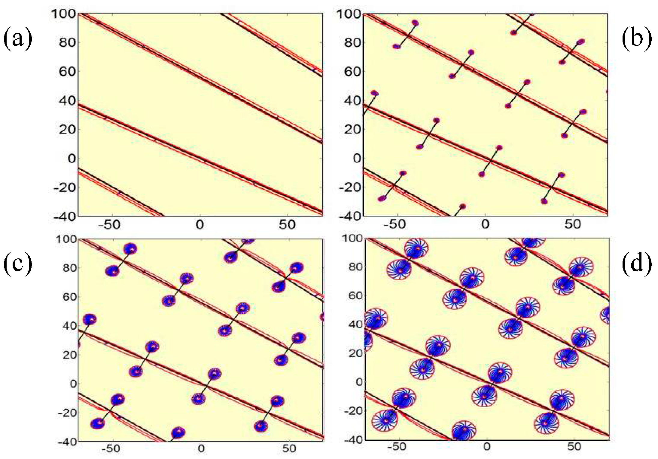
Figure 11.
(a–c) Row 1: Pressure contour maps (in MPa) after 1 month drainage for the same central region of Figure 9d, now including flow through micro-cracks normal to the main fractures. Dipole strength of (a) is scaled to match hydraulic conductivity of the main fractures. Cases (b,c) are respectively 5 and 10 times stronger. (a–c) Row 2: Velocity field (log scale in m·s−1) for cases a-c in Row 1. Local velocities are higher near the micro-crack tips when conductivity is high. Overall area drained stays constant.

Figure 12.
(a–d) Drained region after 1 month of production (red contours). (a) micro-cracks absent, (b,c) micro-cracks with increasing hydraulic conductivity as in Figure 11a–c.
Figure 12.
(a–d) Drained region after 1 month of production (red contours). (a) micro-cracks absent, (b,c) micro-cracks with increasing hydraulic conductivity as in Figure 11a–c.


Table 1.
Key parameters used in this study.
| Hydraulic Fractures Parameters (Equation (27)) | Duong Model: Total Well Strength Parameters (Equations (23–25)) | ||||
|---|---|---|---|---|---|
| Nr. | height hk (ft) | length Lk (ft) | azimuth | Center (ft) | = 9773 (stb/month) |
| 1 | 48.7 | 898 | 122 | 190 + 960 × 1i | = 0 (stb/month) |
| 2 | 53.2 | 1088 | 118 | 105 + 850 × 1i | = 1.133 (1/month) |
| 3 | 63.6 | 1461 | 116 | 135 + 660 × 1i | = 1.2765 |
| 4 | 63.5 | 1134 | 119 | 175 + 445 × 1i | |
| 5 | 67.5 | 1100 | 127 | 70 + 305 × 1i | OOIP parameters (Equations (28) and (29)). |
| 6 | 58.2 | 1223 | 123 | 60 + 145 × 1i | A = 320 acres |
| 7 | 53.6 | 1295 | 118 | 10 − 5 × 1i | h = 57 ft |
| 8 | 56.7 | 1328 | 124 | −60 − 135 × 1i | n = 0.05 |
| 9 | 50.9 | 1248 | 116 | −20 − 350 × 1i | Sw = 0.47 |
| 10 | 49.1 | 1171 | 116 | −325 − 380 × 1i | B = 1.05 |
| 11 | 50.7 | 993 | 112 | −390 − 560 × 1i | |
| 12 | 81.3 | 466 | 105 | −170 − 850 × 1i | Reservoir parameters (for pressure scaling only, cf. Equation (31)) |
| 13 | 49 | 477 | 105 | −170 − 1030 × 1i | Permeability = 1 μD |
| WOR = 1.1659 | Viscosity = 1 cP | ||||
© 2018 by the authors. Licensee MDPI, Basel, Switzerland. This article is an open access article distributed under the terms and conditions of the Creative Commons Attribution (CC BY) license (http://creativecommons.org/licenses/by/4.0/).
Share and Cite
MDPI and ACS Style
Weijermars, R.; Van Harmelen, A. Shale Reservoir Drainage Visualized for a Wolfcamp Well (Midland Basin, West Texas, USA). Energies 2018, 11, 1665. https://doi.org/10.3390/en11071665
AMA Style
Weijermars R, Van Harmelen A. Shale Reservoir Drainage Visualized for a Wolfcamp Well (Midland Basin, West Texas, USA). Energies. 2018; 11(7):1665. https://doi.org/10.3390/en11071665
Chicago/Turabian StyleWeijermars, Ruud, and Arnaud Van Harmelen. 2018. "Shale Reservoir Drainage Visualized for a Wolfcamp Well (Midland Basin, West Texas, USA)" Energies 11, no. 7: 1665. https://doi.org/10.3390/en11071665
Note that from the first issue of 2016, this journal uses article numbers instead of page numbers. See further details here.