Computational Fluid Dynamics Modeling and Validating Experiments of Airflow in a Data Center


Division of Fluid and Experimental Mechanics, Luleå University of Technology, SE-971 87 Luleå, Sweden
*
Author to whom correspondence should be addressed.
Energies 2018, 11(3), 644; https://doi.org/10.3390/en11030644
Submission received: 24 February 2018
/
Revised: 12 March 2018
/
Accepted: 12 March 2018
/
Published: 14 March 2018
Abstract
:The worldwide demand on data storage continues to increase and both the number and the size of data centers are expanding rapidly. Energy efficiency is an important factor to consider in data centers since the total energy consumption is huge. The servers must be cooled and the performance of the cooling system depends on the flow field of the air. Computational Fluid Dynamics (CFD) can provide detailed information about the airflow in both existing data centers and proposed data center configurations before they are built. However, the simulations must be carried out with quality and trust. The k– model is the most common choice to model the turbulent airflow in data centers. The aim of this study is to examine the performance of more advanced turbulence models, not previously investigated for CFD modeling of data centers. The considered turbulence models are the k– model, the Reynolds Stress Model (RSM) and Detached Eddy Simulations (DES). The commercial code ANSYS CFX 16.0 is used to perform the simulations and experimental values are used for validation. It is clarified that the flow field for the different turbulence models deviate at locations that are not in the close proximity of the main components in the data center. The k– model fails to predict low velocity regions. RSM and DES produce very similar results and, based on the solution times, it is recommended to use RSM to model the turbulent airflow data centers.
1. Introduction
During the last several years, the demand on data storage has increased and it will most probably continue to do so in the future. The facilities housing the storage systems are called data centers. As a result of the increased demand, both the number and the size of data centers are expanding rapidly [1]. Since investments in new data centers are likely to continue, developing sustainable solutions is very important. In 2012, the energy consumption for data centers represented about 1.4% of the total energy consumption worldwide, with an annual growth rate of 4.4% [2]. Reducing the energy consumption in data centers will have a major impact on the global energy system already today but even more in the future. As a result of the development of higher power densities for the servers, liquid cooling is introduced as a complement to the traditional air cooling systems in some new data centers [3]. In addition to introducing data centers with new cooling technologies, it is equally important to improve the energy efficiency of the traditional air cooling systems in already existing data centers. This may imply studies on component level [4], rack level [5] and room level [6]. The focus in this study is on the largest of these scales.
The most important parts in a data center are Computer Room Air Conditioner (CRAC) units and server racks housing servers. The servers generate heat and must be cooled to maintain a satisfactory temperature. If the cooling is insufficient, there is a risk of overheating, which might cause the servers to shut down. It is very important that the servers are sufficiently cooled, whereas over-dimensioned cooling systems in data centers are both costly for business and a waste of energy. The CRAC units supply cold air. Ideally, the supplied cold air enters through the front side of the server racks and the hot air that exits through the back side of the server racks returns to the CRAC units. Unfortunately, the exhausted hot air may enter the front side of another server rack instead. This is called hot air recirculation and should be avoided [7]. To avoid hot air recirculation, the server racks are often placed in a number of rows where hot and cold aisles are formed between the rows. Cold aisles are formed between two rows where the front sides are facing each other and hot aisles are formed between two rows where the back sides are facing each other. To further prevent hot and cold air from mixing, aisle containment is a strategy that can be used by either containing the hot aisles or the cold aisles [8]. There are two main categories of configurations in data centers, hard floor configurations and raised floor configurations. In a hard floor configuration, the CRAC units supply the cold air directly into the data center. In a raised floor configuration, the cold air is supplied into an under-floor space instead and enters the data center through perforated tiles located in the cold aisles. Using a raised floor configuration can also be a strategy to prevent unwanted mixing of hot and cold air. There are thermal guidelines that specify recommended and allowable temperature ranges of the air that enters the server racks [9]. The recommended and allowable temperature ranges are 18–27 and 15–32 , respectively. These guidelines apply to data centers in general and are likely to be refined in the future.
The performance of the cooling system in a data center depends on the flow field of the air. Computational Fluid Dynamics (CFD) is an efficient tool to provide detailed information about the airflow. Experimental procedures are more expensive and time-consuming. Another advantage of using CFD modeling is the possibility to analyze proposed data center configurations that have not been built yet, in addition to already existing data centers. However, it is very important that the simulations are carried out with quality and trust. Important parameters such as quality of the computational grid, boundary conditions and choice of turbulence model must be carefully considered [10]. Otherwise, the results from CFD modeling can be misleading.
The Reynolds number is most likely high in large parts of data centers and turbulence must then be taken into account when modeling the airflow. The most common turbulence model used in previous studies concerning CFD modeling of data centers is the k– model [11]. A well-known disadvantage of the k– model is its inability to predict anisotropic turbulence [12]. It also assumes that the flow is fully turbulent, which is inaccurate if the velocities are small in some parts of the data centers. Cruz et al. [13] compared the performance of the k– model to even more simplified turbulence models when modeling the airflow in a data center. As there are no reported results on more advanced turbulence models, a benchmark study on this subject is essential. The aim of this study is to examine the performance of different turbulence models, not previously investigated for CFD modeling of data centers, in a similar manner as described by Larsson et al. [14] for another application. The considered turbulence models are the k– model, the Reynolds Stress Model (RSM) and Detached Eddy Simulations (DES). The commercial code ANSYS CFX 16.0 (ANSYS, Canonsburg, PA, USA) is used to perform the simulations and experimental values are used for validation. All the results are evaluated for the case when RSM is used. The k– model and DES is only used for comparison to RSM.
2. Governing Equations
The governing equations of fluid flows in general are the conservation laws for mass, momentum and energy. In turbulent flows, the instantaneous variables are often decomposed into a mean value and a fluctuating value, where the mean value usually is the most important part. By decomposing the variables in the Navier–Stokes equations and taking the time average, governing equations of the steady mean flow are obtained. They are called the Reynolds-Averaged Navier–Stokes (RANS) equations and read
where are the Reynolds stresses. As shown by the first term on the left-hand side, depending on the choice of time averaging scale, transitions and larger fluctuations in the flow are still allowed. To close the system of equations for the steady mean flow, a turbulence model must be used.
The k– model solves additional transport equations for two variables, turbulent kinetic energy and rate of dissipation of turbulent kinetic energy. It is based on the turbulent-viscosity hypothesis, which assumes isotropic turbulence and proportionality between the Reynolds stresses and the mean velocity gradients according to
There is no assumption on isotropic turbulence for the Reynolds Stress Model (RSM). Instead, it solves additional transport equations for the six individual Reynolds stresses as well as an additional equation for the rate of dissipation. The individual Reynolds stresses are used to obtain closure of the RANS equations. The turbulent-viscosity hypothesis is not needed, which means that one of the major disadvantages with the k– model is eliminated. Detached Eddy Simulation (DES) is a hybrid formulation of RANS (the SST model in ANSYS CFX) inside the boundary layers and Large Eddy Simulations (LES) elsewhere. Turbulent flow contains a wide range of both length and time scales. Scales larger than a predefined filter scale are resolved, whereas only the scales that are smaller than the filter scale are modeled when LES is used. Because the larger-scale motions are represented explicitly, using LES is much more computationally expensive than using other turbulence models [15].
Close to a solid wall, the velocity approaches zero and there is a viscous sublayer. Far away from the wall, viscous forces are negligible compared to inertia forces. Somewhere between these limits there exists a region called the log–law layer, where there is a logarithmic relationship between the dimensionless expressions for velocity and wall distance. Viscous forces and inertia forces are equally important in this region [16]. When it can be assumed that the entire boundary layer does not need to be resolved, a wall function approach can be used in ANSYS CFX . The near-wall grid points should then be located inside the the log–law layer [17].
3. Method
3.1. Geometry
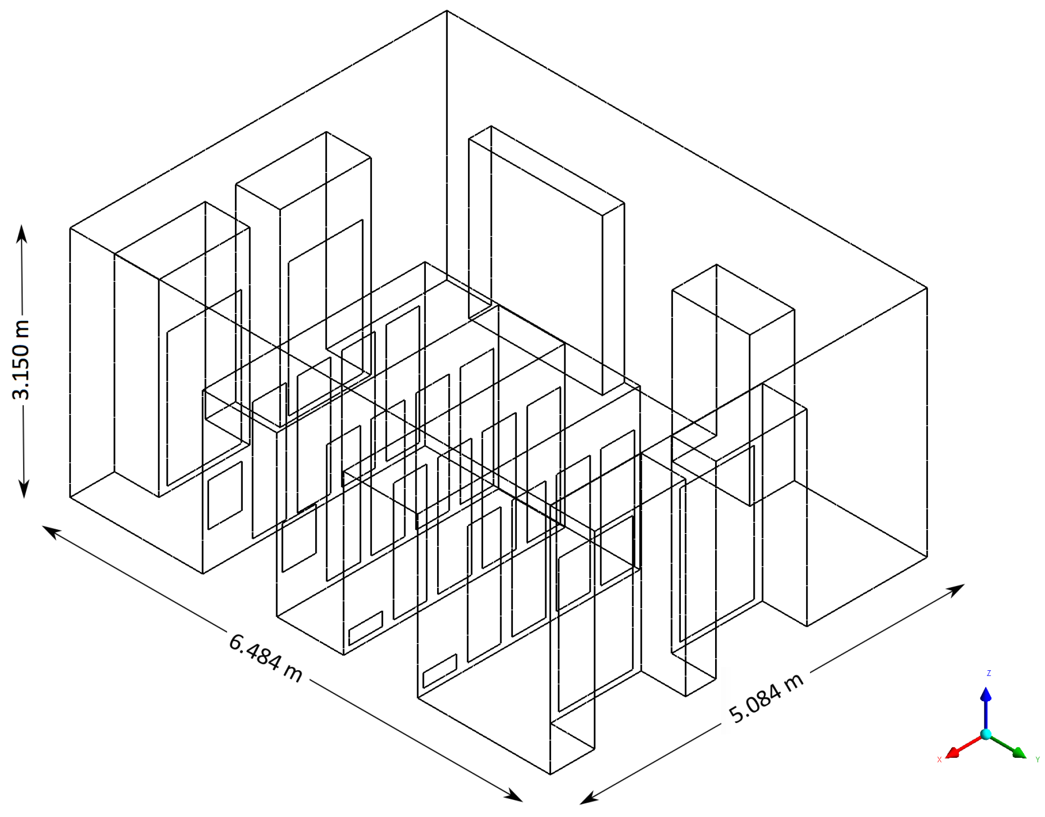
The considered data center is Module 1 at the large-scale research facility SICS ICE, located in Luleå. A traditional air cooling system based on a hard floor configuration is used. The dimensions of the data center are m. Figure 1 shows the geometry in the CFD model, where the main components are four CRAC units and ten server racks. In Figure 2, all the components as well as the locations where velocity measurements have been performed are labeled. A hot aisle is formed between the two rows of server racks, which are positioned with the back sides facing each other. Partial hot aisle containment is imposed by using a door at the end of the rows. SEE Cooler HDZ-2 (SEE Cooling, Nacka, Sweden) and 600 mm wide pre-assambled cabinets (Minkels, Veghel, The Netherlands) are used as CRAC units and server racks, respectively. A full server rack houses 18 PowerEdge R730xd servers (Dell, Round Rock, TX, USA). All server racks are full, except for R5, which is empty but has a small opening that does not contain blanking panels and R6 that houses only six servers. In the simulations, the flow inside the main components was not resolved. Instead, boundary conditions were applied to the sides where the flow enters and exits the CRAC units and the server racks. There are also a switchgear and an uninterruptible power supply (UPS) that were modeled without heat loads. They were included to take the effect of flow blockage into account, but smaller obstructions such as cables and pipes were ignored.
3.2. Grid
The geometry was imported into ANSYS Meshing and tetrahedral grids were created. The discretization error was estimated using the Grid Convergence Index (GCI) and Richardson’s extrapolation [18]. Solutions on three different grids that converge against the same result are required to use the method. The maximum element sizes were chosen in order to obtain a constant refinement factor for the investigated grids. When unstructured grids are used, the refinement factor for two different grids is determined as
where N is the number of elements and D is the number of dimensions. When computed profiles of a variable are used to estimate the discretization error, error bars should be used to indicate numerical uncertainty. This should be done using the GCI with an average value of as a measure of the global order of accuracy [19]. For a constant refinement factor, the order of p is calculated as
where and . , and are the solutions on the coarse, medium and fine grid, respectively. The approximate relative error for the fine grid is
and the fine-grid convergence index is
The extrapolated values are
3.3. Boundary Conditions
The flow rate and the supply temperature must be measured to be able to set up boundary conditions on a CRAC unit. The flow rates through the front sides of all the CRAC units were measured using the DP-CALC Micromanometer Model 8715 and the Velocity Matrix add-on kit from TSI (Shoreview, MN, USA). The Velocity Matrix is designed for area-averaged multi-point face velocity measurements. The accuracy is of reading m/s for the velocity range 0.25–12.5 m/s. The front sides of the CRAC units were divided into smaller regions where the face velocity was measured, and the average velocity was used to set up the inlet boundary conditions. The mass flow rate through the inlets and the outlets located on the CRAC units should be equal. The outlets were located on the top side of the CRAC units. The supply temperature was measured using the handheld hotwire thermo-anemometer VT100 from Kimo (Gothenburg, Sweden). It has an accuracy of of reading for temperatures from to . The measured values for the CRAC units are presented in Table 1.
The flow rate through the server racks must be measured and the heat load generated by the servers must be known to be able to set up boundary conditions on a server rack. The strategy of using boundary conditions at the server racks instead of modeling the flow inside is called the black box model [20]. Zhang et al. [21] compared the black box model to more detailed server rack models and showed that the choice of server rack model does not significantly affect the flow field. The flow rates through all the server racks were measured on the back sides using the same equipment as for the CRAC units. The mass flow rate through the inlet on a server rack and the outlet located on the same server rack should be equal. The total heat load generated at each server rack as well as the measured velocities are presented in Table 2. The heat load results in a temperature difference across the server rack. It is determined as
where q is the heat load, is the mass flow rate and is the specific heat capacity, which was considered constant equal to in the simulations. The temperature at the back side of a server rack was calculated by using this relation in addition to the average temperature on the front of the server rack.
The floor, the walls and the ceiling were assumed to be adiabatic with no-slip boundary conditions, and it was assumed that there was no leakage out of the data center.
3.4. Additional Simulation Settings
Abdelmaksoud et al. [22] showed that the effect of buoyancy often should be taken into account in CFD modeling of data centers. Buoyancy is the driving force for natural convection. The importance of buoyancy is quantified by the Archimedes number, a ratio of natural and forced convection. It is expressed as
where L is a vertical length scale, is the temperature difference between hot and cold regions, V is a characteristic velocity, g is acceleration of gravity and is the volumetric expansion coefficient. An Archimedes number of order 1 or larger indicates that natural convection dominates. In this study, and the effect of buoyancy should be taken into account. The full buoyancy model in ANSYS CFX was used to calculate the buoyancy force directly from the density variations in the airflow.
Airflows in ventilated rooms cannot be expected to be steady and in some cases, and it is only possible to obtain a converged solution with transient simulations [23]. Airflows in data centers are similar. As could be expected, steady-state simulations had difficulties converging due to fluctuations in the flow field. Therefore, transient simulations were considered instead and the time averaged flow fields were used in the analysis. A constant time step equal to s was applied, but s was required when DES was used as turbulence model. The convergence criteria were such that all the root mean square residuals fall below at each time step. The chosen time step required about three inner iterations per time step. To monitor the progress of the solution and ascertain that the transient simulations reach a statistically steady state, values of velocity and temperature were recorded at the measurement locations. These locations were chosen since they are used both to validate the simulations and to compare the different turbulence models. The simulations were run as long as necessary for the transient averages of both velocity and temperature at all these locations to converge. The simulations were run 60 s as a start-up period and transient averages were then recorded for 600 s. Running the simulations even longer did not change the transient averages, which verifies that this period is sufficient.
3.5. Validation
Velocity and temperature measurements were performed in order to be able to validate the simulations. Velocity measurements were done using the single point anemometer ComfortSense Mini (Dantec, Skovlunde, Denmark). The omnidirectional 54T33 Draught probe (Dantec, Skovlunde, Denmark) was used since it is suitable for indoor applications such as testing of ventilation components. The accuracy is of reading m/s for the velocity range 0.05–1 m/s and of reading for the velocity range 1–5 m/s. Measurements were performed at five different locations in the data center and at three or four different heights for each location (see Figure 2). Values were recorded for 60 s with a sampling frequency of 10 Hz. The average values were the same for longer durations and the sampling frequency was considered to be sufficient to evaluate the time averaged velocity profiles. If evaluation of turbulent quantities would have been of interest, a higher sampling frequency might have been required. Temperature measurements were done using the temperature sensor DPX2-T1H1 from Raritan (Somerset, NJ, USA). It has an accuracy of for temperatures from to . The sensors were placed 1.09 m above the lower edge of the server rack doors on both sides of all server racks.
4. Results and Discussion
4.1. Grid Refinement
The discretization error was estimated using the GCI and Richardson’s extrapolation. The method requires simulations on three different grids. The number of elements are 298,535, 668,242 and 1,486,077 for the coarse, medium and fine grid, respectively. A constant refinement factor of was obtained by setting the maximum cell size for each grid. The maximum cell sizes are 14.0 cm, 10.6 cm and 8.0 cm for the coarse, medium and fine grid, respectively. Five inflation layers with a growth factor of 1.2 are used for all grids to achieve a better resolution near the walls.
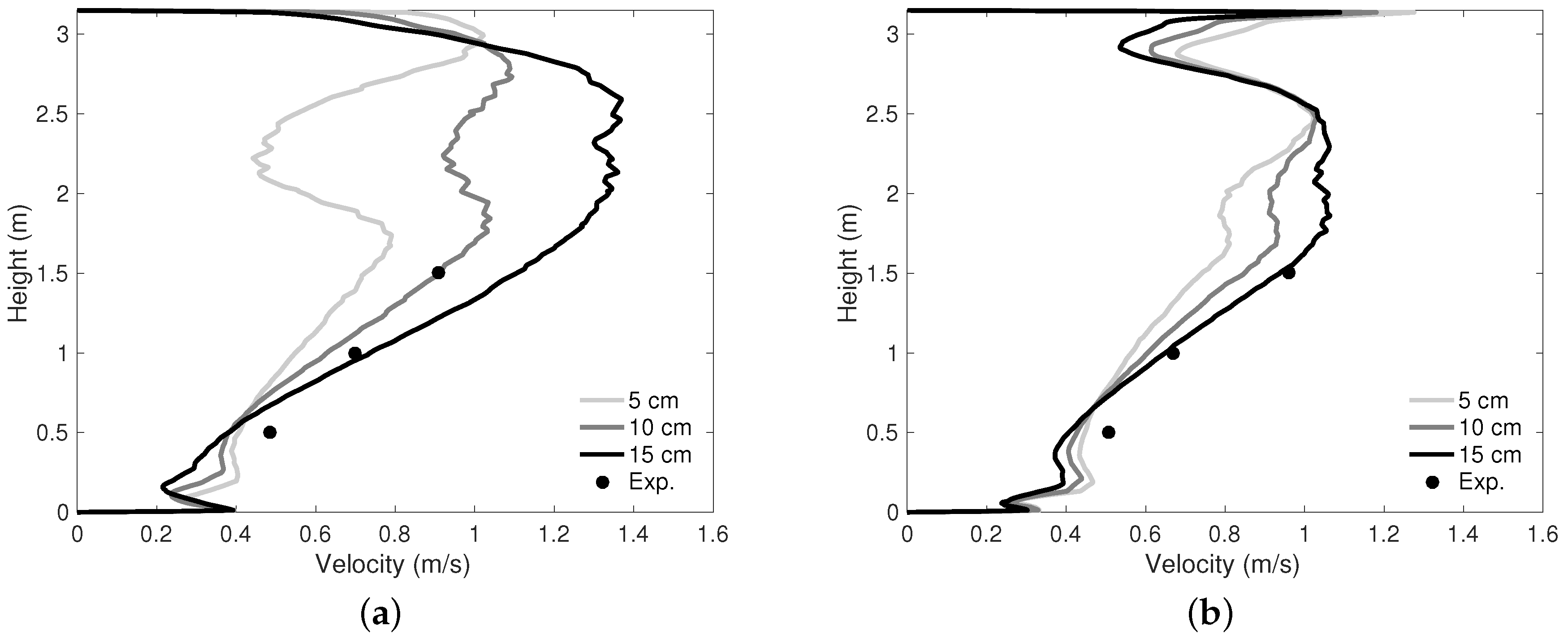
Velocity is one of the most interesting variables of airflow in a data center. Transient averages of velocity profiles along L1 (see Figure 2) are compared for the case when RSM is used as turbulence model. Figure 3a shows velocity profiles for the three investigated grid sizes and an extrapolated curve based on these three different grids according to Richardson’s extrapolation. The local order of accuracy p ranges from 0.0197 to 27.70, with a global average of 6.583. Figure 3b shows error bars for the fine grid, calculated using the GCI with the average value of p. The maximum discretization uncertainty is 0.0521 m/s. Since the fine grid gives acceptable results according to the grid refinement study, all further work in this study is performed using this grid. Using the fine grid is also consistent with previous results regarding grid size for CFD modeling of data centers. VanGlider et al. [24] has shown that results are not totally grid independent even for a grid size as small as 2.5 cm, but do not change significantly below a grid size of about 15.2 cm. However, a significant difference is that hexahedral grids were used in that study.
4.2. Flow Field
To illustrate the flow field of the air, Figure 4 shows streamlines based on the instantaneous velocity field originating from the inlet surfaces located on the CRAC units and the server racks separately. The color of the streamlines represents velocity. Figure 4a shows that a large part of the cold air enters the front side of the server racks, which is the idea, but some fraction returns to the CRAC units instead of reaching the servers. This fraction is higher for C1 and C3, the CRAC units closest to the end of the rows, than for C2 and C4. In total, the CRAC units supply more cold air than necessary for the current setup of server racks. Figure 4b shows that the airflow turns upwards in the hot aisle and stays close to the ceiling while it returns to the CRAC units. No hot air recirculation is apparent over the server racks and the risk of hot air recirculation around server racks is eliminated by the partial hot aisle containment. To illustrate the spatial distribution of the flow field, Figure 5 shows transient averages of velocity, temperature and turbulent kinetic energy on a plane through the center of the rows of server racks. It is even more clear here that both the highest velocities and most of the heat are found close to the ceiling. This is of practical importance for heat re-use applications. It is also obvious that there are large areas with very low velocities that have no function for the cooling. The turbulent kinetic energy is largest at the borders of the jets formed when the hot air moves back to the CRAC units. This is expected and similar to what is revealed in previous studies [25,26].
4.3. Temperatures
A comparison of temperatures at the server racks for the case when RSM is used as turbulence model and experiments is shown in Figure 6. The comparison is made where the temperature sensors are located. Figure 6a shows the temperatures at the front side of the server racks. All the values predicted by the CFD model are within the experimental error bars and well below both the maximum recommended and the maximum allowable temperature specified by the thermal guidelines for data centers. Figure 6b shows the temperatures at the back side of the server racks. In this case, all values except for two are within the experimental error bars. In the simulations, Equation (9) is used to calculate the temperature difference across each server rack. A uniform temperature is applied on the whole inlet surface on the back side of each server rack, respectively. In the experiments, one sensor at each server rack is used to measure the temperatures. However, there are non-uniformities on the back side of the server racks, which the sensors are not able to capture. It may explain the differences found between simulations and experiments. The deviations indicate that using the black box model as boundary condition for the server racks might not give exact results on rack level, which means right behind the server racks. However, it could still give accurate results on room level where the non-uniformities have leveled out. This is further investigated by comparing the velocity profiles from simulations and experiments.
4.4. Velocity Profiles
A comparison of transient averages of velocity profiles for the different turbulence models and experiments is shown in Figure 7. The simulations show that the different turbulence models give different agreement between them and to the experiments depending on the location in the data center. The same tendencies are found for temperatures. Figure 7a–c show the velocity profiles at the measurement locations behind the server racks, inside the hot aisle. As expected, higher velocities are experienced further away from the floor in this region since the airflow turns upwards inside the hot aisle. The velocities are under-estimated by the simulations at L1 and L2, especially at the two upper measurement points. At L3, the velocities produced by the simulations show much better agreement to the experiments. The considered turbulence models produce similar results behind the server racks. The largest difference between the turbulence models are found at heights above the server racks, where the boundary conditions applied to the server racks have less effect on the flow field. The velocity profiles at L4, outside the door at the end of the hot aisle, are shown in Figure 7d. At this location, the flow field is not as affected by the boundary conditions as the flow field at the other measurement locations and some differences between the turbulence models are apparent. Figure 7e shows the velocity profiles at L5, in front of one of the CRAC units. Very good agreement is found between simulations and experiments at this location. It indicates that the simplified boundary conditions that are used to model the CRAC units and server racks give accurate results on room level.
The under-estimated velocities at L1 and L2 are a result of very steep velocity gradients at these locations in a similar manner as for the mid-plane illustrated in Figure 5. Therefore, the distance from where the inlet condition is applied at the back side of the server racks to the location where the measurements are made is very crucial for the results. Velocity profiles from the simulations slightly closer to the center of the hot aisle show much better agreement to the experimental values. To exemplify, Figure 8 shows transient averages of velocity profiles for L1 and L2 when these locations are moved 5 cm, 10 cm and 15 cm in the direction towards the center of the hot aisle. There is very good agreement 10 cm closer to the center for L1 and 15 cm closer to the center for L2. In the considered data center, the back side of the servers does not reach the back side of the server racks. There are gaps behind the server rack doors that are not considered when setting up the boundary conditions. It may explain why the velocities are under-estimated close the the server racks in the simulations.
To further investigate the differences between the turbulence models found at heights above the server racks, Figure 9 shows transient averages of velocity on planes at L1 and L2. It is shown that wakes appear above the outlets located on the back sides of the server racks. The absence of flow from the server racks closest to the wall attracts air exhausted by the other server racks, imposing asymmetry in the flow in the hot aisle. The largest wakes are observed above the server racks in the middle. RSM and DES produce very similar results, but the k– model under-estimates the size of these large low velocity regions. The assumption of fully turbulent conditions is a well-known disadvantage of the k– model. It might explain why inaccurate results are produced in the low velocity regions. The fact that the turbulence models produce different results, even though they all use the wall function approach in ANSYS CFX instead of resolving the boundary layer, indicates that the differences arise from the treatment of the free flow and not the treatment of the boundary layer.
Transient averages of turbulent kinetic energy on planes at L1 and L2 are illustrated in Figure 10 for the case when RSM is used as turbulence model. Most turbulent kinetic energy is created close to the corner where the roof meets the wall and where the flow is deflected. This can be avoided with another design in the data center. When compared to the velocity field in Figure 9, it can also be seen that there is some turbulent kinetic energy in the large wakes. It may be a result of the higher velocity fields next to the wakes. However, it must be remembered that in the middle plane between the server racks there is a jet moving upwards. This jet and the shear created by it may also create the turbulent kinetic energy seen on the planes at L1 and L2.
5. Conclusions
In this study, CFD modeling was used to provide detailed information about the airflow in a data center and experimental values were used for validation. It is intended to contribute to improved accuracy and reliability of CFD modeling of data centers. The simulations must be carried out with quality and trust. The effect of buoyancy must be taken into account when modeling the airflow. The simplified boundary conditions used in this study might not give exact results on rack level, which means right in front of the inlet surfaces located on the components. However, it is indicated that the results on room level are accurate. The aim of this study was not only to validate the CFD model, but also to compare the performance of the different turbulence models. It is clarified that the flow field for the different turbulence models deviate at locations that are not in the close proximity of the main components in the data center. Of the three models compared, the deviations from experimental values are about the same, but differences are found at heights above the server racks. The k– model fails to predict the low velocity region found there. RSM and DES produce very similar results, but the solution time increases significantly when using DES. Therefore, this study indicates that RSM should be used to model the turbulent airflow in data centers. For future studies, measurements should be performed at more locations where the flow field is not as affected by the boundary conditions as it was for many of the measurement locations in this study.
Acknowledgments
The authors would like to acknowledge the Swedish Energy Agency for their financial support and SICS North for providing data and facilities for the experiments.
Author Contributions
Emelie Wibron, Anna-Lena Ljung and T. Staffan Lundström conceived and designed the experiments; Emelie Wibron and Anna-Lena Ljung performed the experiments; Emelie Wibron performed the simulations and analyzed the data; Emelie Wibron wrote the paper; All authors read and approved the final manuscript.
Conflicts of Interest
The authors declare no conflict of interest.
References
- Jiacheng, N.; Xuelian, B. A review of air conditioning energy performance in data centers. Renew. Sustain. Energy Rev. 2017, 67, 625–640. [Google Scholar] [CrossRef]
- Van Heddeghem, W.; Lambert, S.; Lannoo, B.; Colle, D.; Pickavet, M.; Demeester, P. Trends in worldwide ICT electricity consumption from 2007 to 2012. Comput. Commun. 2014, 50, 64–76. [Google Scholar] [CrossRef]
- Ebrahimi, K.; Jones, G.F.; Fleischer, A.S. A review of data center cooling technology, operating conditions and the corresponding low-grade waste heat recovery opportunities. Renew. Sustain. Energy Rev. 2014, 31, 622–638. [Google Scholar] [CrossRef]
- Ventola, L.; Curcuruto, G.; Fasano, M.; Fotia, S.; Pugliese, V.; Chiavazzo, E.; Asinari, P. Unshrouded Plate Fin Heat Sinks for Electronics Cooling: Validation of a Comprehensive Thermal Model and Cost Optimization in Semi-Active Configuration. Energies 2016, 9, 608. [Google Scholar] [CrossRef]
- Fakhim, B.M.; Srinarayana, N.; Behnia, M.; Armfield, S.W. Thermal Performance of Data Centers-Rack Level Analysis. IEEE Trans. Compon. Packag. Manuf. Technol. 2013, 3, 792–799. [Google Scholar] [CrossRef]
- Wibron, E.; Ljung, A.-L.; Lundström, T.S. CFD simulations comparing hard floor and raised floor configurations in an air cooled data center. In Proceedings of the 12th International Conference on Heat Transfer, Fluid Mechanics and Thermodynamics, Malaga, Spain, 11–13 July 2016; pp. 450–455. [Google Scholar]
- Patankar, S.V. Airflow and Cooling in a Data Center. J. Heat Transfer 2010, 132, 073001. [Google Scholar] [CrossRef]
- Tatchell-Evans, M.; Kapur, N.; Summers, J.; Thompson, H.; Oldham, D. An experimental and theoretical investigation of the extent of bypass air within data centres employing aisle containment, and its impact on power consumption. Appl. Energy 2017, 186, 457–469. [Google Scholar] [CrossRef]
- ASHRAE Technical Committee. 2011 Thermal Guidelines for Data Processing Environments–Expanded Data Center Classes and Usage Guidance. Available online: http://ecoinfo.cnrs.fr/IMG/pdf/ashrae_2011_thermal_guidelines_data_center.pdf (accessed on 23 May 2017).
- Misiulia, D.; Andersson, A.G.; Lundström, T.S. Computational Investigation of an Industrial Cyclone Separator with Helical-Roof Inlet. Chem. Eng. Technol. 2015, 38, 1425–1434. [Google Scholar] [CrossRef]
- Fulpagare, Y.; Bhargav, A. Advances in data center thermal management. Renew. Sustain. Energy Rev. 2015, 43, 981–996. [Google Scholar] [CrossRef]
- Larsson, I.A.S.; Lindmark, E.M.; Lundström, T.S.; Nathan, G.J. Secondary Flow in Semi-Circular Ducts. J. Fluids Eng. 2011, 133, 101206. [Google Scholar] [CrossRef]
- Cruz, E.; Joshi, Y. Inviscid and Viscous Numerical Models Compared to Experimental Data in a Small Data Center Test Cell. J. Electron. Packag. 2013, 135, 030904. [Google Scholar] [CrossRef]
- Larsson, I.A.S.; Lundström, T.S.; Marjavaara, B.D. Calculation of Kiln Aerodynamics with two RANS Turbulence Models and by DDES. Flow Turbul. Combust. 2015, 94, 859–878. [Google Scholar] [CrossRef]
- Pope, S.B. Turbulent Flows, 1st ed.; Cambridge University Press: Cambridge, UK, 2000; ISBN 0521598869. [Google Scholar]
- Versteeg, H.K.; Malalasekera, W. An Introduction to Computational Fluid Dynamics: The Finite Volume Method, 2nd ed.; Pearson Prentice Hall: Harlow, UK, 2007; ISBN 0131274988. [Google Scholar]
- ANSYS. ANSYS CFX-Solver Theory Guide, 16th Release; ANSYS: Canonsburg, PA, USA, 2015. [Google Scholar]
- Roache, P.J. Perspective: A Method for Uniform Reporting of Grid Refinement Studies. J. Fluids Eng. 1994, 116, 405–413. [Google Scholar] [CrossRef]
- Celik, I.B.; Ghia, U.; Roache, P.J.; Freitas, C.J.; Coleman, H.; Raad, P.E. Procedure for Estimation and Reporting of Uncertainty Due to Discretization in CFD Applications. J. Fluids Eng. 2008, 130, 078001. [Google Scholar] [CrossRef]
- Zhai, J.Z.; Hermansen, K.A.; Al-Saadi, A. The Development of Simplified Boundary Conditions for Numerical Data Center Models. ASHRAE Trans. 2012, 118, 436–449. [Google Scholar]
- Zhang, X.; VanGlider, J.W.; Iyengar, M.; Schmidt, R.R. Effect of rack modeling detail on the numerical results of a data center test cell. In Proceedings of the 11th IEEE ITHERM Conference, Orlando, FL, USA, 28–31 May 2008; pp. 1183–1190. [Google Scholar]
- Abdelmaksoud, W.A.; Khalifa, H.E.; Dang, T.Q. Improved CFD modeling of a small data center test cell. In Proceedings of the 12th IEEE ITHERM Conference, Las Vegas, NV, USA, 2–5 June 2010; pp. 1–9. [Google Scholar]
- Nielsen, P.V. Fifty years of CFD for room air distribution. Build. Environ. 2015, 91, 78–90. [Google Scholar] [CrossRef]
- VanGlider, J.W.; Zhang, X. Coarse-Grid CFD: The effect of Grid Size on Data Center Modeling. ASHRAE Trans. 2008, 114, 166–181. [Google Scholar]
- Benard, N.; Balcon, N.; Touchard, G.; Moreau, E. Control of diffuser jet flow: turbulent kinetic energy and jet spreading enhancements assisted by a non-thermal plasma discharge. Exp. Fluids 2008, 45, 333–355. [Google Scholar] [CrossRef]
- Karabelas, S.J.; Koumroglou, B.C.; Argyropoulos, C.D.; Markatos, N.C. High Reynolds number turbulent flow past a rotating cylinder. Appl. Math. Model. 2012, 36, 379–398. [Google Scholar] [CrossRef]
Figure 1.
Geometry of the data center in the CFD model.

Figure 2.
Labeled CRAC units, server racks and measurement locations.

Figure 3.
Velocity profiles along L1 for (a) all the different grids and (b) the fine grid with error bands. RSM is used as turbulence model.
Figure 3.
Velocity profiles along L1 for (a) all the different grids and (b) the fine grid with error bands. RSM is used as turbulence model.

Figure 4.
Streamlines originating from (a) the CRAC units and (b) the server racks when RSM is used.
Figure 4.
Streamlines originating from (a) the CRAC units and (b) the server racks when RSM is used.

Figure 5.
Velocity, temperature and turbulent kinetic energy on a plane through the center of the rows of server racks when RSM is used.
Figure 5.
Velocity, temperature and turbulent kinetic energy on a plane through the center of the rows of server racks when RSM is used.

Figure 6.
Temperatures at (a) the front side and (b) the back side of the server racks. RSM is used as turbulence model in the CFD model.
Figure 6.
Temperatures at (a) the front side and (b) the back side of the server racks. RSM is used as turbulence model in the CFD model.

Figure 7.
Velocity profiles at (a) L1; (b) L2; (c) L3; (d) L4; and (e) L5.

Figure 8.
Velocity profiles when moving (a) L1 and (b) L2 closer to the center of the hot aisle.

Figure 9.
Velocity on planes at (a) L1 and (b) L2 for the k– model, (c) L1 and (d) L2 for RSM and (e) L1 and (f) L2 for DES.
Figure 9.
Velocity on planes at (a) L1 and (b) L2 for the k– model, (c) L1 and (d) L2 for RSM and (e) L1 and (f) L2 for DES.

Figure 10.
Turbulent kinetic energy on planes at (a) L1 and (b) L2 for RSM.


Table 1.
Boundary conditions for the CRAC units.
| CRAC Unit | Velocity | Temperature |
|---|---|---|
| C1 | ||
| C2 | ||
| C3 | ||
| C4 |
Table 2.
Boundary conditions for the server racks.
| Server Rack | Velocity | Heat Load |
|---|---|---|
| R1 | ||
| R2 | ||
| R3 | ||
| R4 | ||
| R5 | ||
| R6 | ||
| R7 | ||
| R8 | ||
| R9 | ||
| R10 |
© 2018 by the authors. Licensee MDPI, Basel, Switzerland. This article is an open access article distributed under the terms and conditions of the Creative Commons Attribution (CC BY) license (http://creativecommons.org/licenses/by/4.0/).
Share and Cite
MDPI and ACS Style
Wibron, E.; Ljung, A.-L.; Lundström, T.S. Computational Fluid Dynamics Modeling and Validating Experiments of Airflow in a Data Center. Energies 2018, 11, 644. https://doi.org/10.3390/en11030644
AMA Style
Wibron E, Ljung A-L, Lundström TS. Computational Fluid Dynamics Modeling and Validating Experiments of Airflow in a Data Center. Energies. 2018; 11(3):644. https://doi.org/10.3390/en11030644
Chicago/Turabian StyleWibron, Emelie, Anna-Lena Ljung, and T. Staffan Lundström. 2018. "Computational Fluid Dynamics Modeling and Validating Experiments of Airflow in a Data Center" Energies 11, no. 3: 644. https://doi.org/10.3390/en11030644
Note that from the first issue of 2016, this journal uses article numbers instead of page numbers. See further details here.