ACT-R Cognitive Model Based Trajectory Planning Method Study for Electric Vehicle’s Active Obstacle Avoidance System


1
School of Automotive Engineering, Shan Dong Jiao Tong University, Jinan 250357, China
2
Energy and Power Engineering College, Nanjing University of Aeronautics & Astronautics, Nanjing 210016, China
*
Authors to whom correspondence should be addressed.
Energies 2018, 11(1), 75; https://doi.org/10.3390/en11010075
Submission received: 27 October 2017
/
Revised: 9 December 2017
/
Accepted: 21 December 2017
/
Published: 1 January 2018
(This article belongs to the Special Issue The International Symposium on Electric Vehicles (ISEV2017))
Abstract
:The active obstacle avoidance system is one of the important components of the electric vehicle active safety system. In order to realize the active obstacle avoidance system driving the vehicle smoothly and without collision in complex road situation, a new dynamical trajectory planning method based on ACT-R (Adaptive Control of Thought-Rational) cognitive model is introduced. Firstly, the ACT-R cognitive architecture is introduced and the trajectory planning method’s framework structure based on ACT-R cognitive model is built. Secondly, the modeling method of ACT-R cognitive model is introduced, the main module of ACT-R cognitive model includes the initialized behavior module, trajectory planning module, estimated behavioral module, and weight adjustment behavior module. Finally, the verification of the trajectory planning method is conducted by the simulation and experiment results. The simulation and experiment results showed that the method of AR (ACT-R) is effective and feasible. The AR method is better than the methods that are based on the OC (Optimal Control) and FN (fuzzy neural network fusion); this paper’s method has more human behavior characteristics and can meet the demand of different constraints.
1. Introduction
In recent years, under the double pressure of energy and environment, electric vehicles became the focus of the automobile industry. With the rapid development of electric vehicles, the fatal traffic accidents of electric vehicle occur frequently, which makes the traffic safety issues become the focus of attention, where the rear-end accidents accounted for the most of the traffic accidents. So the avoidance of rear-end accidents becomes the present urgent problems [1,2]. Electric vehicle active collision avoidance system is one of the most effective methods to solve the rear-end accidents and it is a driving assistant system that is based on vehicle active safety technology. It is effective to improve driving safety by installing some sensors in the car [3,4]. We can know the environment and status with the sensors to assist driver driving, for example, avoiding obstacles and preventing accidents from happening actively. The main function of active collision-avoidance system is pre-alarming or independent braking, but the independent steering is rarely used in the collision-avoidance system [5]. The statistics suggested that about 40% of the collisions occurred in the vehicle’s tail [6], so the active steering is effective to avoid rear-end collisions and the combination of active steering and brake will improve the vehicle’s active safety in many cases. In the higher relative speed driving condition of the vehicle, the active steering is the best method of obstacle avoidance. In emergency case, the drivers must make decisions of steering in a very short time and the steering angular must be very accurate, but all of these actions of the driver under complex road condition are pretty difficult to achieve [7].
In the electric vehicle’s active collision-avoidance system, the controller can help the driver to follow the right way and improve the driving stability. The controller’s design is a difficult problem in the research [8,9]. Lou etc. [10] got the parameters of controller by the trajectory planning method based on dynamics, the controller is used to control the motor torque, so the industrial robot motion control is realized. Goodarzi etc. [11] introduces three layers vehicle dynamics controller to control the DC hub motor of the wheel-motor electric vehicle. Among them, the higher-level controller can provide the angular velocity and the traveling speed of the vehicle, the mediate-level controller can provide the traction and yaw moment, the lower-level controller can provide the torque of the wheels. The controller will be decoupled of trajectory planning and motion control in the paper, the trajectory planning is used to provide real-time effective trajectory and the trajectory’s characteristic values [12], including the vehicle’s speed, acceleration, driving time, electricity consumption, and other state and control parameters [13,14]. The trajectory’s characteristic values will be sent to the low-level controller of active avoidance system. After receives detailed information of the trajectory, the controller will control the vehicle to drive along the planned trajectory to avoid obstacles.
The existing trajectory planning method is mainly used different functions to simulate the trajectory, such as B-spline function, polynomial function, sine function and arc etc. The electric vehicle is applied a variety of constraints, the feasible trajectories that meet the constraints is generated [15,16]. In the conventional method, the trajectory’s parameters cannot achieve the function which can dynamic adjust online, so the generated trajectory cannot adapt to continuously changing road condition dynamically. The different digital constraints are applied to the evaluation function in the optimal control (OC) methods to get the optimal driving trajectory. But, the OC methods only deal with the digital constraints, the soft constraints of natural language cannot be processed [17]. Some optimization methods of fuzzy logics and neural networks can handle natural language, but this algorithm is too complex and it is not very well to deal with the constraints of human behavioral characteristics, thus the specific application is limited [18,19]. The existing methods are not precise enough to express the driver’s behavior characteristics.
The cognitive science is the intellectual revolution’s frontier subject in the 21st Century, it is mainly study human’s cognitive process, intelligence system and internal operating mechanism of the brain. ACT-R is a new cognitive architecture of cognitive science, the model established in the ACT-R reflects human’s cognitive behavioral characteristics [20]. The cognitive system are mainly includes ACT-R [21,22] and EPIC (Executive Process Interactive Control) [23] etc., all of this cognitive system can not only build the model of people’s cognitive behavior, but also build the model of human’s cognitive process that want to achieve the desired objectives [24,25]. This paper chooses ACT-R, because ACT-R has the sub-symbolic system, which can be used in the trajectory planning method [26]. The ACT-R cognitive system is the core in the literature [27] and the driving behavior is built model used ACT-R, this proved that the cognitive behavior modeling method based on ACT-R is very suitable and flexible. In this paper, ACT-R cognitive models and numerical calculation method based on state space is linked together and the ACT-R cognitive model is the core. The method of dynamic adjustment evaluation function’s different weights value is used to generate suitable running trajectory according to different road environments. Human’s cognitive behavioral characteristics are used in the trajectory planning method and the generated trajectory can meet different constraints and human’s cognitive characteristics. Finally, the simulation and experiment of different methods are conducted to test this paper method’s superiority.
2. The ACT-R Cognitive Architecture
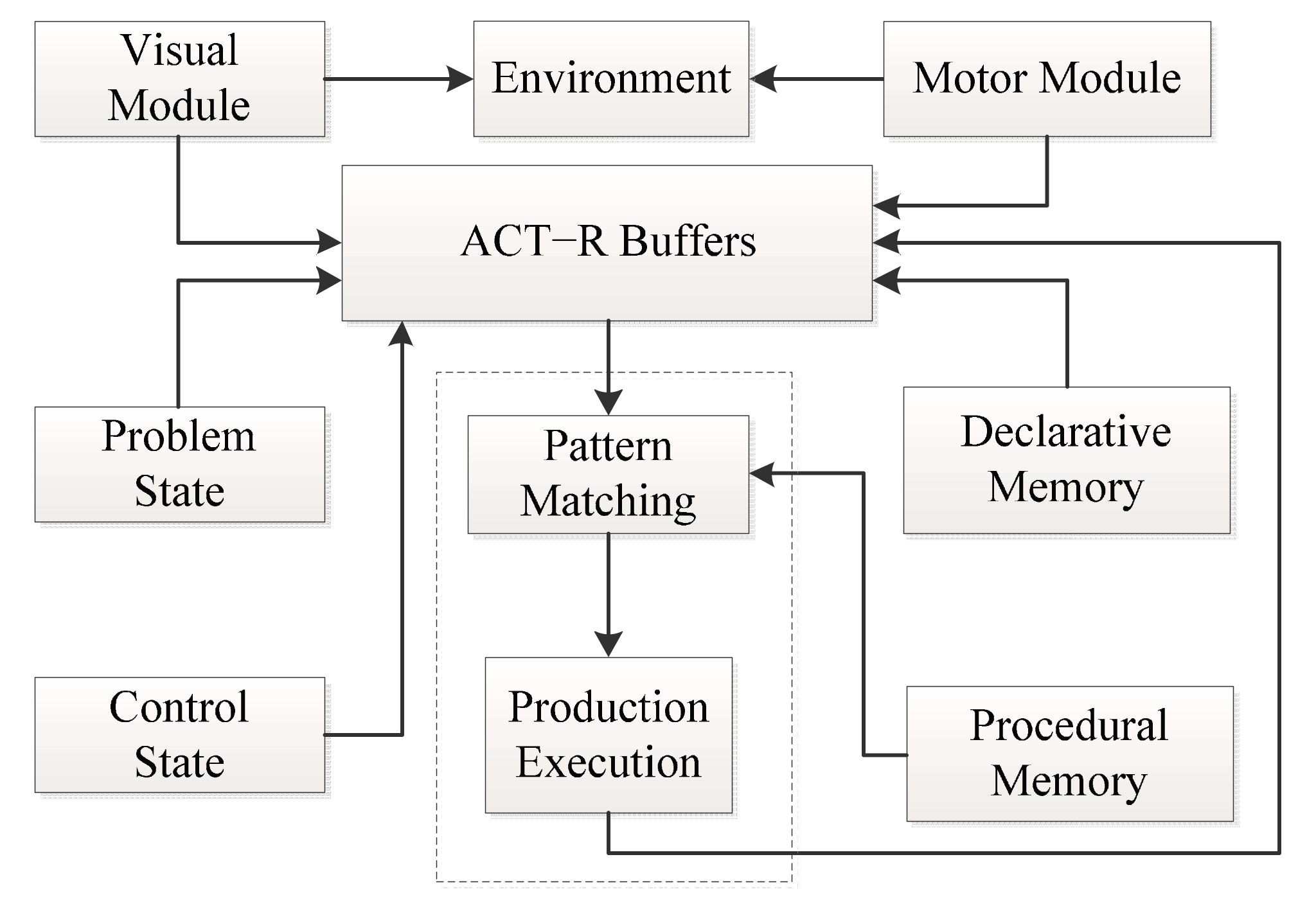
ACT-R is a cognitive architecture. It is a theory of the structure of the brain at a level of abstraction that explains how it achieves human cognition. It consists of a set of independent modules that acquire information from the environment, process information, and execute motor actions in the furtherance of particular goals. Figure 1 illustrates the main components of the architecture.
There are three modules that comprise the cognitive components of ACT-R. The three modules are basic module, buffer, and pattern matching modules. The basic modules have two types: Memory module and vision-motor module. The memory module mainly includes: declarative memory module, procedural memory module and goal stack. The vision-motor module includes vision and motor modules, the visual and motor modules provide ACT-R with the ability to simulate visual attention shifts to objects on a computer display and manual interactions with a computer keyboard and mouse.
The declarative memory module also called declarative knowledge, the declarative knowledge is the knowledge that we can understand and can describe to the others. In ACT-R, the declarative knowledge is expressed as “chunk” structure, and can form declarative memory; it shows that human might have knowledge in problem solving, such as “George Washington was the first President of the United States”. The procedural memory module also called procedural knowledge, it reflects the fact that how to deal with declarative ability to solve the problem. Procedural knowledge generation process are essentially a conditioned reflex triggered rules when condition is met. Procedural knowledge is compiled through “production rules”. The declarative memory module can store factual knowledge about the domain, and the procedural memory module can store the system’s knowledge about how tasks are performed. The former consists of a network of knowledge chunks, while the latter is a set of production rules of the form “if <condition> then <action>”: the condition specifying chunks that must be present for the rule to apply and the action specifying the actions to be taken should this occur.
Each of ACT-R’s modules has an associated buffer that can hold only one chunk of information from its module at a time and the contents of all the buffers constitute the state of an ACT-R model at any one time. Cognition proceeds via a pattern matching process that attempts to find production rules with conditions that match the current contents of the buffers. When a match is found, the production “fires” and the actions are performed. Then the matching process continues on the updated contents of the buffers so that tasks are performed through a succession of production rule firings.
Except the symbolic level mechanisms, ACT-R also has a sub-symbolic level of computations that govern memory retrieval and production rule selection. The retrieval process based on activation, a chunk in declarative memory has a level of activation, which determines its availability for retrieval, the level of which reflects the frequency of its use. This need models to account for widely observed frequency effects on retrieval and forgetting. Sub-symbolic computations also govern the probability of productions being selected in the conflict resolution process. It is assumed that people choose the most efficient actions to maximize the probability of achieving the goal in the shortest amount of time. The more often a production is involved in the successful achievement of a goal, the more likely it will be selected in the future.
3. The Frame Structure of the Trajectory Planning Method Based on ACT-R
When the driver is driving, the behavior characteristics can be described by some emotional language, for example carefully, slowly, and careless, etc. When the ACT-R cognitive model is working with the driver, the cognitive model can accept and deal with the driver’s language symbolic information and estimate the trajectory’s modified quantity to meet the driver’s need. When the ACT-R worked alone, the generated trajectory can self-evaluation and the trajectory’s eigenvalues and related constraints is compared to estimate the trajectory’s eigenvalues. If the eigenvalues meet requirements, then the generated trajectory is returned to the drivers, if the eigenvalues cannot meet requirements, ACT-R can make hominine decision to decide the variable quantity of the trajectory’s characteristic value and weight value.
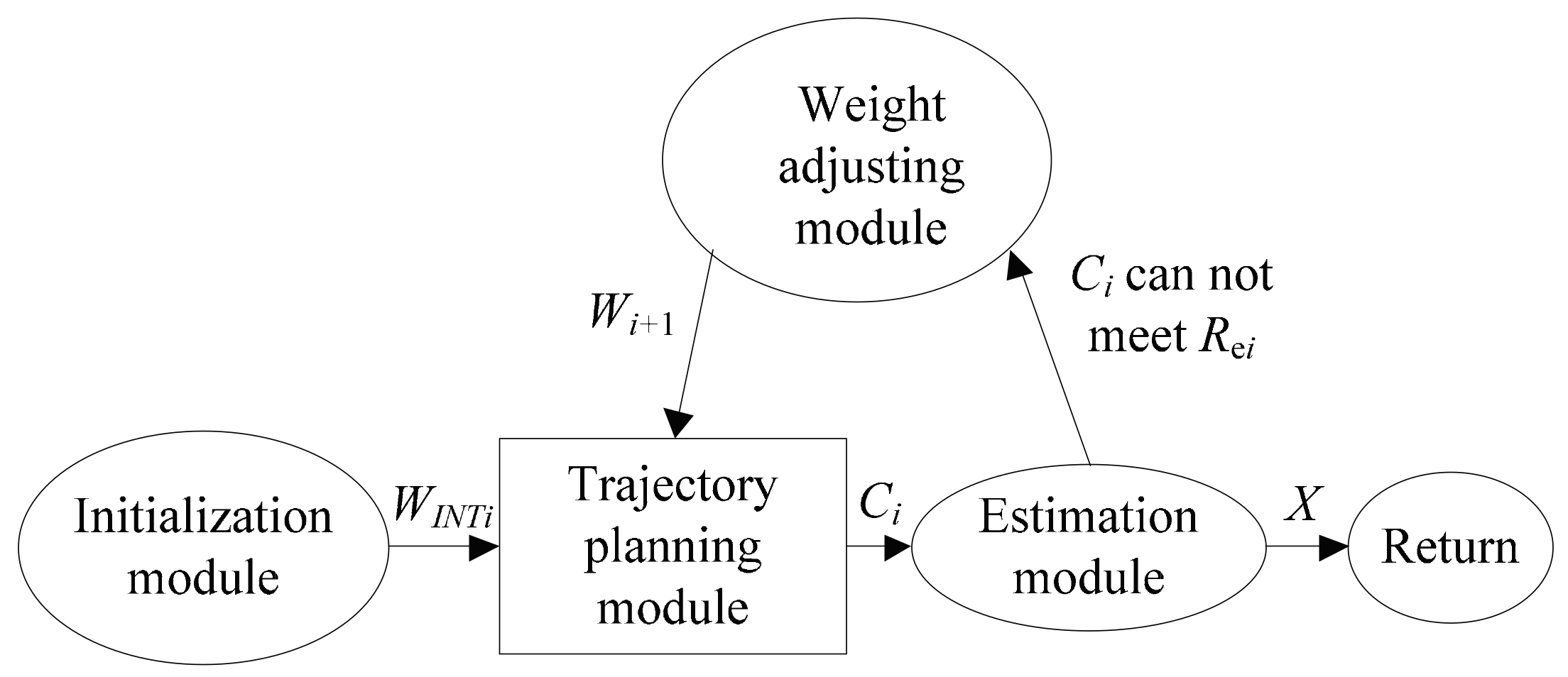
The frame structure of the trajectory planning method based on ACT-R cognitive model can be shown in Figure 2.
The trajectory planning method includes initialization module, trajectory planning module, weight adjusting module, and estimation module, where except for the trajectory planning module, the other three modules are based on the ACT-R cognitive model. The detailed instruction of the method’s framework structure is shown as follows: Firstly, the trajectory planning problem P0 is initialized by initialized module, secondly, the trajectory is generated by trajectory planning module, the trajectory’s characteristics Ci is extracted and transferred to estimated module. The estimated module judges whether all of the trajectory’s characteristics can meet the constraints Re, if the trajectory’s characteristics meet the constraints, the solution X can be return to the behavior decision system, if the trajectory’s characteristics cannot meet the constraints, the weight adjustment module is called to adjust the weight and the adjusted weight sets Wi+1 can be supplied to trajectory planning module to generated trajectory again, the circulation is proceeded repeatedly, the suitable solution X can be found and supplied to the controller.
4. The Modeling Method of ACT-R Cognitive Model
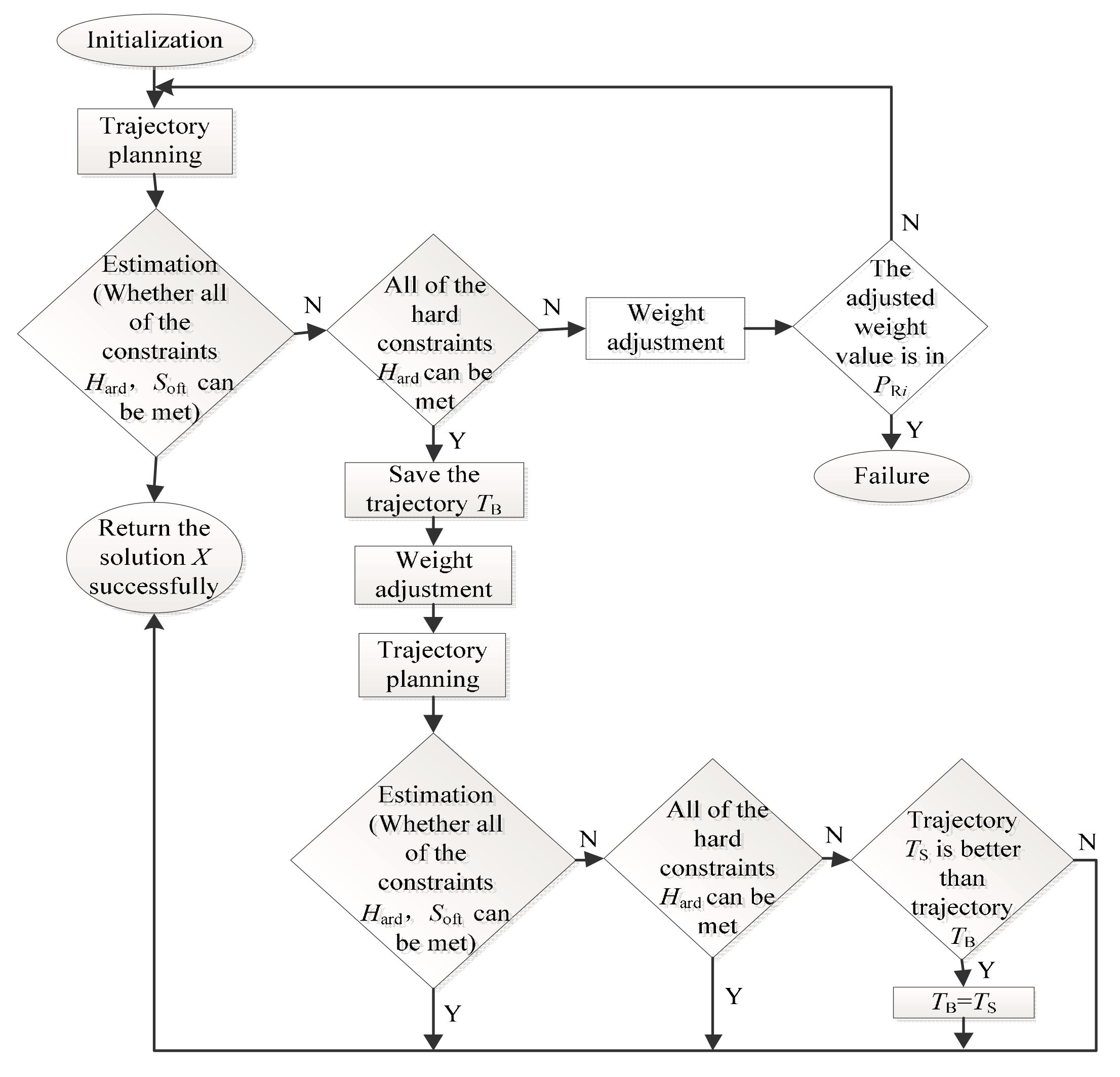
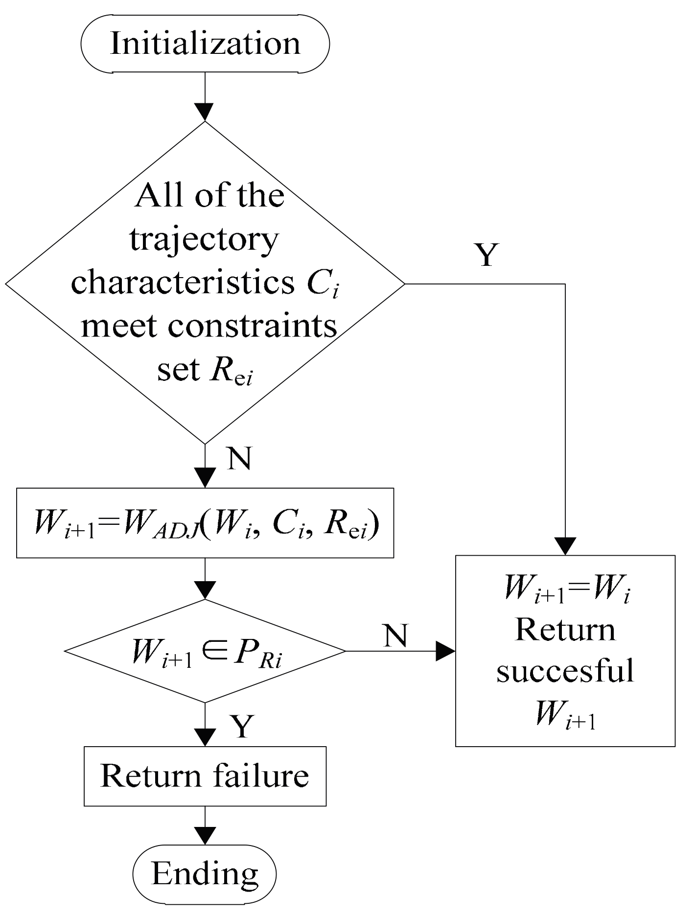
The trajectory planning method flow chart based on ACT-R cognitive model is shown in Figure 3. Firstly, the trajectory planning problem is initialized by the Initialization module, then the trajectory is generated by the trajectory planning module and the trajectory’s characteristic values are sent to estimation module to estimate. The estimation module can judge if the trajectory’s characteristic values meet the constraints, the constraints include hard constraints Hard (i.e., “u > 30 m/s”) and soft constraints Soft, the soft constraints Soft includes adverb constraints (i.e., quickly) and numerical value constraints (i.e., 100 km/h ≤ uavg ≤ 160 km/h). If the trajectory and trajectory’s characteristic values satisfy the constraints, the solution method X = {Jn, Ren, tn, xn, un} is returned to behavior decision system, where, Jn and Ren summarize the solution cost and the feature constraints, respectively, and the set {tn, xn, un} specifies the full-state trajectory to be executed. If the trajectory and trajectory’s characteristic values cannot satisfy the constraints, the property of the constraints should be analyzed. If the hard constraints Hard is not satisfied, then the weight adjusted module is called to adjust the weight and the new weight Wi+1 is generated. The estimation module need to detect the weight adjusted history {PRi}, if the new weight Wi+1 is not in the weight adjusted history set {PRi}, the weight adjustment is success; if the new weight Wi+1 is in the weight adjusted history set {PRi}, then the weight adjustment is failure. The adjusted process is running until the trajectory characteristic values meet the hard constraints. The trajectory TB that meets the hard constraints but cannot meet the soft constraints is saved to ensure the trajectory that meets the hard constraints can be output. Then the second cycle is done, the trajectory TB’s characteristic values that has been saved is been adjusted, and the new adjusted weight value is estimated by the estimation module, the estimation module will judge if the trajectory’s characteristic value satisfy all of the constraints, if all of the constraints are met, then the successful solution X is output; if only the hard constraint Hard can be met, then the solution X is output; if the hard constraint Hard cannot be met, then the trajectory TS will be compared to the trajectory TB. If the trajectory TS can satisfy the constraint conditions more than trajectory TB, then the TB will be replaced by TS in the memory.
We can determine which trajectory is better through the error vector calculation, the smaller error range is the optimal trajectory, the error vector of the ith iteration, and jth trajectory characteristic is shown as Formula (1):
where, is the ith iteration and jth trajectory characteristic value, is the jth trajectory characteristic value’s constraint condition, means the trajectory characteristic meet the related constraint condition, means the trajectory characteristic does not meet the related constraint condition. According to the trajectory planning’s ith iteration, the jth trajectory characteristic value is compared with the jth constraint condition. If the smaller constraint condition cannot meet, the ’s value is negative; if the bigger constraint condition cannot meet, the ’s value is positive. If the constraint condition is a numerical range, then the numerical range’s boundary value will be used to calculate, the ’s value can decide the weight adjusted orientation.
4.1. ACT-R Initialized Behavior Modeling
According to the different driving environment, the trajectory module can generate the trajectory based on the state-space trajectory planning method. The BVP (Boundary Value Problem) can be solved by function BVP4C solution. Although the problem of driving’s terminal time is free can be solved by BVP4C solution, but if the initial evaluated value is not rational, then the results may be not convergence. So, the trajectory’s initial weight set WINT (i.e., [1, 1, 1, 3]) should be evaluated, ACT-R cognitive model is the core of the ACT-R initial module, the information of driving region boundary of the vehicle, goal, and constraints can be encoded and changed into some needed information that can generate trajectory and initial weight set WINT, if the constraints are not exit, then the weight value WDefault (i.e., [1, 1, 2, 5]) is supposed as the default weight set.
In the initial process, the disposed method of the upper limit and lower limit of numerical range soft constraints Soft (i.e., 100 km/h ≤ uavg ≤ 160 km/h) is just as the hard constraints Hard (i.e., uavg > 30 m/s). The numerical value constraints of the soft constraints or hard constraints can be described using symbolic language, such as “30 m/s < u < 40 m/s” can be described as “the maximum speed is higher”, so the disposing method is the same as the adverb soft constraints Soft’ disposing method.
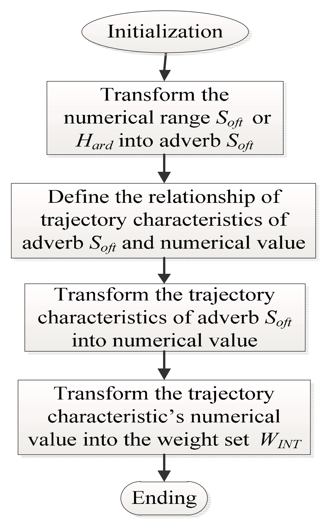
The deterministic method of the initial weight set WINT can be shown in Figure 4. The initial process is shown as follows: Firstly, transform the numerical value constraints of the soft constraints Soft (i.e., 100 km/h ≤ uavg ≤ 160 km/h) or hard constraints Hard (i.e., u > 20 m/s) into the adverb Soft (i.e., quickly); Second, the relationship of trajectory characteristics (i.e., umax, uavg and amax) and adverb soft constraints Soft are defined, such as the adverb Soft “slowly”, is related to trajectory characteristics “low” maximum speed umax and “low” average speed uavg. Then, according to the relationship definition (just as Table 1) of trajectory characteristics and numerical value, the description of “higher” maximum speed and “higher” average speed can be expressed by some numerical value range, such as “high” maximum speed’s range is [100, 120]; Finally, according to the weight adjusted regulation rule Table 2, the trajectory characteristic’s numerical value range is corresponding to the weight value range, for example, the numerical value range of W3/W1 is (0.25, 0.5], that is corresponding to the maximum speed’s numerical value range [80, 100]. All of the process can call the ACT-R’s procedure knowledge module, the specific production rule set Z is the production rule set, the form of the set is “if <condition> then <action>”, i.e., “if 0 ≤ W3/W1 ≤ 0.125 then 100 km/h ≤ uavg ≤ 160 km/h”, the specific production rule set Z is shown in Table 2. Thus, the constraints Soft and Hard can be transformed into initial weight set WINT. If the constraints are not exit, then the weight value WDefault is supposed as the default weight set.
4.2. Trajectory Planning Module
The trajectory planning module takes as input the initial weight vector WINT, and it as cost-functional terms. The trajectory planning module can return a full state trajectory, including position, velocity, and control inputs at each time step. Because the trajectory planning method that we used is based on human cognitive behavior characteristic and human driver is very suitable for control of linear systems, but has not very good control of nonlinear system, so the vehicle’s model in this paper is supposed as a simple linear dynamic model, the simplified two-dimensional linear dynamical model is expressed as Equation (2),
where, m is the object mass, cs is the friction coefficient, u(t) is the control input variable, x(t) is state vector,
is the vehicle’s velocity vector, and is the vehicle’s acceleration vector. Let , then the Equation (2) can be converted to Equation (3),
The trajectory generation module uses the OC method to plan the trajectory. The aim is finding out the available control input variables u(t)* and making the system (3) follow the feasible trajectory x1(t)* that can minimize evaluation function (4),
where, t is the driving time, (t) is state vector, and is its derivative, u(t) is the control input, t0 and tf is the vehicle’s initial time and end time, respectively. According to all of the t[t0, tf], the state condition of fixed starting point and end point, the boundary conditions are as Formula (5),
where, x0 and xf is the vehicle’s location when the vehicle driving in the time t0 and tf, respectively.
x0(t0) = x0, x1(tf) = xf
There are three evaluation indexes in the OC method that should be optimized; the evaluation indexes are energy, time, and the shortest distance that far away from the obstacle. The evaluation function of Formula (4) can be expressed as Formula (6), the weight vector Wi = [W1, W2, W3, LIM], the description of each evaluation index are as follows,
where, W1 is the weight of driving time, because evaluation function J is the integral form in the time quantum [t0, tf], so we need a constant coefficient W1 to optimize the time; W3 is the weight of energy, the expression of energy is simplified, u2(t) express the energy, the u(t) is controlled quantity; W2 is the weight of the shortest distance far away from the obstacle, the term is added to keep he vehicle drive away from the obstacles, bi(ri) is a compensation function, when the vehicle driving near the obstacle center i, the compensation function value increases, on the contrary, when the vehicle driving far away from the obstacle, the compensation function value decreases, ri is the distance between the vehicle and the obstacle’s center i, the value of compensation function bi(ri) is maximum value MAX over the center of the obstacle, attains fixed value K at the obstacle boundary a distance Ri from the obstacle center and decreases to zero at a distance LIM away from the obstacle’s edge, these constraints and the smoothness conditions of the function smooth are described by Equation (7). The third-order polynomial function bi(ri) that meets these constraints was selected and the value of bi(ri), is meaningful only if ri < LIM, the third-order polynomial function bi(ri) is shown, just as Equation (8),
where, the value of MAX and K can be got by means of the experiment, the value of bi(ri) is equal to K when the vehicle is touching the obstacle. The coefficients ci (i = 1, …, 8) can be found by solving the two third-order equations and their first and second derivatives to satisfy all of the smoothness constraints of Equation (7).
Thus, the Formula (6) can be changed into the problem of solving the integral constant when the boundary conditions are given. The BVP4C in MATLAB can be a numerical solver to solve the problem and the complete trajectory can be generated. The dynamical model and evaluation function can be linked, thus the trajectory considering the dynamical constraints is feasible.
After generating the trajectory, the trajectory characteristic value Ci can be extracted and it is sent to the estimation module for estimating. The trajectory characteristic value is the whole trajectory’s digital property, the same as the trajectory characteristic value’s quantification. The feature extraction is a computational procedure, the generated trajectory is the input variable, the useful trajectory characteristic value can be extracted as the estimation of the trajectory, such as the driving time, energy, maximum speed, and maximum acceleration are the typical trajectory features. Some trajectory features is the mean and percent of the whole trajectory characteristic values. Such as, smooth time is a time period that the vehicle’s speed, acceleration, and rotational speed’s fluctuation cannot exceeding the whole scope’s 1%, this is the trajectory characteristic value’s numerical approximate value and the velocity’s constant degree is estimated.
The trajectory’s main constraint conditions can be divided into numerical constraints and language description constraints. The numerical constraints include hard constraints and soft constraints. In general, the numerical constraint is a numerical range that has the upper and lower limits, in other words, the hard constraint’s characteristic value is greater or less than one fixed value, the soft constraint’s characteristic value is between two numerical values. The soft constraint is mainly represented by linguistic description, such as the linguistic description “quickly” or “slowly”. When such descriptive language is used, then the different description language can be transformed into some linguistic symbols that ACT-R can recognize, such linguistic symbols can be used by making correspondence relationship’s definition between linguistic symbols and the trajectory’s characteristic values, such as “quickly” can correspond with “high” maximum speed and “high” maximum acceleration.
4.3. ACT-R’s Estimated Behavioral Modeling
Estimation module is a core part of ACT-R cognitive model [28] and it determines which production rule is selected to use. According to estimated behavioral modeling, some parameters’ values should be expressed by described knowledge. Such as different trajectory feature values Ci = {C1, C2, C3, } with each Ci described by different trajectory’s characteristics, such as umax, uavg, amax, etc., i.e., C1 = {umax = 100 km/h, uavg = 50 km/h, amax = 6 m/s2), constraints set Rei = {Re1, Re2, Re3, } with each Rei described by hard constraints Hard and soft constraints Soft, i.e., Re1 = {Hard = [umax < 110 km/h], Soft = [quickly]}, weight set Wi is defined as [W1, W2, W3, LIM], Wi+1 is the adjusted weight set which has the same form with Wi, i.e., Wi = [1, 1, 3.6, 5], historical weight set PRi = {PR1, PR2, PR3, } with each PRi described by an action Ai and trajectory planning state Si, for trajectory planning problem, action set Ai is defined as {Initialization, Trajectory-planning, Estimation, eight-adjustment}, and trajectory planning state Si is defined as the full-state trajectory {tn, xn, un} to be executed. All of the parameters can be described with descriptive language. The decision-making process can be expressed by procedural knowledge, namely the production rule. The procedural knowledge of estimation module can be shown in Table 3.
In estimation module’s pattern matching process, the current goal “declarative knowledge” is given and one of the “production rules” is chose to match the current goal through the conflict resolution method. The sub-symbolic (i.e., numerical) information that is associated with the production rules is used to determine which production rule is selected to use. During the model runs, the number of successes and failures of each production rule is recorded by the module. In addition, estimation module records the efforts (e.g., time) that are spent after executing the rule and actually achieving the goal (or failing). This information is used to estimate empirically the probability of success Pi and the average cost Li of each production rule, the success Pi of Equation (9) and the average cost Li of Equation (10), just as follows,
where is the number of success, is the number of failure, is the sum of all the costs, associated with previous tests of the ith rule, , where is the number of previous tests of rule i. When the goal is completed, aiming at a production rule, the estimation module would update the production rule’s number of success or failure. For example, if cost is measured in time units, then Equation (10) calculates the average time for exploring particular decision trajectory. By this way, the probabilities and costs of rules are learned by the estimation module.
ACT-R uses numerical methods to solve this problem. Each production rule has an expected return Ni in the ACT-R. When several production rules compete in the conflict set, ACT–R calculates their expected returns by the following equation:
where F is the goal value, is a random number taken from a normal distribution with zero mean and variance . Finally, the rule of Equation (12) is selected according to expected return’s maximization,
Ni = PiF − Li + ξ(σ2)
The flow of estimation module is shown in Figure 5. All of the features Ci extracted by feature extraction module is compared with constraints set Rei generated by the initialization module, when all of the features Ci within the range Rei, the new weight value Wi+1 = Wi, and the successful Wi+1 is returned. When it is not within the scope of Rei, in order to meet the requirements of the constraint set Rei, the estimation module need to call the weight adjustment module to adjust trajectory weights. When the trajectory characteristic values Ci are compared with the constraint set Rei, estimation module compared new weight Wi+1 with the historical weight set PRi, if the new weights Wi+1 is in the set PRi, the result of weight adjustment is wrong; if there are not new weight values, then the original weight values Wi is right and if new weight value Wi+1 is not in the set PRi, the new weight value Wi+1 = Wi and the successful Wi+1 is returned. Because of the memory and learning ability, ACT-R model is able to remember the previous invalid choice to avoid ineffective iteration loop.
When the estimation module calls weight adjustment module, it is necessary to make sure of the input parameter of the weight adjustment module, including the unsatisfied constraint conditions, the difference value between the actual trajectory feature values and the limitation value and how to adjust to meet the limit requirement more easily. Decision-making system may impose incompatible constraints on the planned trajectory. At this time, estimation module should inform a decision-making system that it is impossible to meet its requirements. According to the conflict resolution method, estimation module can intelligently decide which constraint is easier to meet and which trajectory is close to the decision making system’s requirement. Once the estimation module finds the trajectory that can meet all of the constraints, the returning module would return the trajectory to decision making system.
4.4. The ACT-R Weight Adjustment Behavior Modeling
In the trajectory planning method based on the space state, the relationship between right trajectory feature values and weight adjustments method has been obtained. In this method, the trajectory’s feature values can be adjusted to meet constraints by adjusting weight value. But, the generated trajectory may not meet human’s behavior characteristics. The aim of weight adjust module is adjusting weight to meet human’s behavior characteristics according to the vehicle driving environment and constraints. For example, if energy consumption weight and the shortest distance from the barrier weight is larger, then the vehicle can drive slowly, avoid rapid acceleration, and stay away from obstacle. If the weight of time is larger, the car will speed up, avoid the obstacle with high speed, and close to the obstacle. We can name the trajectory features with emotional language, such as careful and bold.
The weight ratio value W3/W1 is not accurate and it is the exponential form base 2: 2−3, 2−2, 2−1, 20, 21, 22, 23. Because human’s cognition behavior is vague, so the accuracy of the weight ratio value does not affect the algorithm’s results. The languages symbol “very low” and “very high” is used to classify define weight ratio W3/W1 reasonable. The relative weight ratio W3/W1 and trajectory characteristic’s descriptive knowledge are shown in Table 1 and Table 4.
In order to link weight ratio W3/W1 and trajectory characteristics, the detailed relationship can reference the literature [29], for characteristics relating to time (e.g., velocity, acceleration, energy), strong relationships between the characteristics value and the time-term weight (W3/W1) is as follow
where, exponent −λ is approximately constant within a certain area, constant coefficient q1 is changing constantly, and it can be calculated by the trajectory characteristics value and the real value of W3/W1. Similarly, for trajectory-based features, such as minimum separation from obstacles dmin, there is a linear relationship between the feature and the influence limit LIM:
where LIM is simply the distance over which the obstacle penalty function goes to zero, as measured from the edge of the obstacle, q2 is constant coefficient Rather than attempt to calculate tables for all of the possible constant coefficients q1 and q2 of these equations for all possible field sizes, they are computed online, using the current weight and feature values to back out the coefficient value. The coefficient, together with the desired feature value (e.g., the limit, if it was passed), are then used to re-compute the weights and the weights’ online adjusting is completed.
dmin = q2LIM
The weight ratio and trajectory characteristics are described by descriptive knowledge, the detailed introduction is shown as Table 2 and Table 3, respectively. For example, according to Table 2, if the weight ratio value W3/W1 is “low”, then we can see how to definite the maximum acceleration amax that corresponding with “low” weight ratio value W3/W1. We can see from Table 3 that the maximum acceleration amax’s definition is “high”. So we can get the corresponding relationship between the weight ratio and trajectory characteristics, in other words, we can get weight adjustment’s procedural knowledge, just as shown in Table 4. The corresponding relationship between the weight ratio and the trajectory characteristics can be divided into two kinds. One is positive related and the other is inversely related. In the proportional related example, “very low” weight ratio value can result in “very low” characteristic value and “low” weight ratio value can result in “low” characteristic value. In the inversely related example, “very low” weight ratio value can lead to “very high” characteristic value. According to time-related trajectory characteristic values, the descriptive knowledge of weight ratio value W3/W1 is related to the descriptive knowledge of trajectory characteristic value. According to distance related trajectory characteristic value, for example, the values of minimum distance dmin and LIM, the default LIM’s “intermediate” value is 3, LIM is defined as linear related with shortest distance.
When the vehicle drives in the dynamic scene, the rolling planning method is used to make the trajectory planning real-timely. According to the environment, the trajectory is planned in one sampling period using this paper’s method and the trajectory is planned again using this paper’s method in the next sampling period, the process of rolling planning cycle until the vehicle complete the whole journey. In every sampling period, the trajectory’s sensors can obtain the real-time information around the vehicle, the information is relative to time and distance and the information is also called trajectory feature value Ct (i.e., the distance from the obstacles d and the driving time t), the real-time trajectory feature value is sent to estimation module, and the estimation module compare the real-time trajectory feature value with the constraint condition, if the constraint condition cannot be met, then the estimation module would call the weight adjustment module to adjust the weight values to meet the constraints, the new weight values Wi will be calculated, the process is running until the feasible weight value is found and the optimized trajectory is generated using the feasible weight value in the trajectory planning module. The detailed process is introduced as follows:
When the trajectory optimized process is running, the initial weight set WINT can be sent to trajectory planning module and the trajectory can be generated using the trajectory planning module, the vehicle will drive along the planned trajectory, then the real-time trajectory characteristic value Cti (i.e., umax = 30 m/s) can be obtained using the sensors and sent to estimation module. In estimation module, the trajectory characteristic value Cti can be compared with the constraints Rej (i.e., 30 m/s < u < 40 m/s), if the constraint condition can be met, the trajectory can be returned, the trajectory optimized process is successful; if the constraint condition cannot be met, then the weight adjustment module would be called to adjust the weight values to meet the constraints, the new weight values Wi+1 will be calculated. For example, if the maximum speed umax cannot meet the constraints “umax < 40 m/s”, because the maximum speed umax is a trajectory characteristic that is related to time, so the Equation (11) is used to calculating. The detailed compute procedure can be shown as follows: Firstly, in Equation (11), the value of λ is constant in a certain range, the real-time characteristic value umax is known, the weight ratio W3/W1 is known according to the WINT, so the value of q1 can be calculated. Secondly, according to the Equation (11) , the trajectory characteristic value gets from the constraints as the ideal characteristic value Ct, the value of q1 are also known, so the new weight ratio W3/W1 can be calculated. The circulation process is running until the feasible weight value is found.
5. The Simulation Analysis of the Trajectory Planning Method
The simulation analysis used this paper’s trajectory planning method is done based on ACT-R cognitive model (abbreviation: AR) and the traditional OC method that is the method based station spaced (abbreviation: OC), respectively. The OC is the method based station spaced and the method can generate optimal trajectory for the intelligent vehicle to complete the ability of collision-avoidance in different obstacles environment. The AR is a method combined with ACT-R and OC. The OC is the traditional trajectory planning method, the ACT-R cognitive model is not used in the OC. To be more clear, the method AR is mainly based on the ACT-R cognitive model and the method has human’s cognitive characteristic, while the OC is mainly based on station space, it is a numerical calculation method. The architecture of AR included initialization module, estimation module, trajectory planning module, and weight adjustment module, while the architecture of OC only has the trajectory planning module and weight adjustment module and the weight adjustment module run in Matlab instead of ACT-R. The OC is completed in the software Matlab and CarSIM, while the method AR is completed in the software ACT-R, Matlab and CarSIM.
The aim of the simulation is to test the superiority of this paper’s trajectory planning method AR. The simulation environment is the obstacle environment with 4 different obstacles {Bi} {i = 1, 2, 3, 4} and the constraints are Rei{i = 1, 2, 3, 4, 5}. The detailed simulation method of AR is as follows: Firstly, according to the constraints, the initial weight set is generated by ACT-R’s initial module, and the initial weight set is sent to Matlab, then, the trajectory is generated by the trajectory planning module based on the initial weight value in Matlab and the vehicle drives along with the generated trajectory in CarSIM, Finally, the trajectory’s characteristic values are extracted in CarSIM and the characteristic values are sent to the estimation module of ACT-R. The ACT-R’s estimation module can judge the trajectory’s characteristic value whether it meets the constraint conditions, if the characteristic values cannot meet the constraint condition, the ACT-R’s weight adjustment module is called to adjust the weight value. The weight adjustment process is done until the characteristic values meet all the constraint conditions. The detailed simulation method of AR is as follows: Firstly, according to the constraints, the default weight set WDfault is sent to Matlab, then, the trajectory is generated by the trajectory planning module based on the default weight set WDfault in Matlab and the vehicle drives along with the generated trajectory in CarSIM, Finally, the trajectory’s characteristic values are extracted in CarSIM and the characteristic values are sent to the weight adjustment module in Matlab. The weight adjustment module can adjust the weight value to meet the constraints based on the weight adjustment rule. The weight adjustment process is done until the characteristic values meet al.l the constraint conditions.
Suppose that the vehicle’s driving velocity is higher in the simulation, so the vehicle’s dynamical model is considered, the dynamical model use the simplified linear dynamical model, the dynamical model is as Formula (2). Suppose that the intelligent vehicle is electric drive, about 20 times simulation analysis is done to test this paper’s method. The vehicle’s driving region is 200 m × 150 m, the driving time is 10 s, and the obstacle set {Bi} is as follows:
- {B1} = {(160, 40), 3}
- {B2} = {[(26, 23), 5], [(32, 13), 5], [(70, 66), 5], [(108, 55), 7], [(135, 111), 7], [(83, 55), 7], [(160, 99), 2.5]}
- {B3} = {[(25, 35), 5], [(50, 80), 2.5], [(120, 120), 10]}
- {B4} = {[(16, 4), 2], [(30, 10), 2.5], [(30, 20), 5], [(80, 60), 7], [(100, 80), 5], [(120, 90), 6], [(150, 100), 3]}
The constraint set is as follows:
- Re1 = {Soft = [a bit fast], [very curious]}
- Re2 = {Hard = [umax < 110 km/h], Soft = [quickly]}
- Re3 = {Hard = [umax > 110 km/h, amax ≤ 0.2 g], Soft = [80 km/h ≤ uavg ≤ 100km/h, appropriate safely]}
- Re4 = {Hard = [umax < 100 km/h, amax ≤ 2 m/s2], Soft = [80 km/h ≤ uavg ≤ 100km/h]}
- Re5 = {Hard = [dmin ≥ 3 m, amax ≤ 25 m/s2], Soft = [safely]}
The constraint set Re1 includes two soft constraints, the constraints set Re3 includes two hard constraints, one soft numerical value constraint, and one soft language constraint.
In the 20 times simulation analysis, the two trajectory planning methods begin run based on the weight set WDz0 = [1, 1, 1, 1] generated by the state space trajectory planning method and the weight set WDa0 = [15, 3, 1, 1] generated by the trajectory planning method based on ACT-R cognitive model, respectively. Where, the four weights of the weight set are time, the distance away from the obstacle, energy and limit LIM. The second constraint set Re2 includes hard constraint condition umax < 110 km/h and soft constraint condition “quickly”, the soft constraint condition “quickly” can extend to high maximum speed umax and average speed uavg, the same as Soft = {100 km/h ≤ umax ≤ 120 km/h, 85 km/h ≤ uavg ≤ 100 km/h}. In the 20 times simulation analysis, when the vehicle drives in the obstacle set {B2} and constraint set Re2, the weight adjust result is shown in Table 5 and Table 6. Where, umax is the vehicle’s maximum speed, uavg is the vehicle’s average speed, WDzi{i = 1, 2, 3}, and WDai{i = 1, 2} express weight set’s numerical value of different iterative process. Dzi{i = 0, 1, 2} and Dai{i = 0, 1} express each iterative calculative result in the weight adjust process.
We can see from Table 5 that the trajectory characteristic value umax = 115.25 km/h what is generated by WDz0 cannot satisfy the hard constraint condition umax < 110 km/h and uavg = 110.36 km/h cannot satisfy soft constraint condition 85 km/h ≤ uavg ≤ 100 km/h, so the weight that is related to time should be adjusted. The adjusted weight is weight set WDz1, the trajectory characteristic value of average speed generated by adjusted weight set WDz1 uavg = 105 km/h cannot meet the constraint condition 85 km/h ≤ uavg ≤ 100 km/h, so in the next weight adjust process Dz2, the weight that is related to the time would be adjusted again. The trajectory characteristic values generated by adjusted weight set in the iteration Dz2 can meet all of the constraints. We can see from Table 6 that, the trajectory characteristic values generated by weight set WDa0 cannot meet the average speed constraint condition 85 km/h ≤ uavg ≤ 100 km/h, because the intelligent vehicle in order to meet the constraint condition “quickly”, the speed is more quickly, so the average speed constraint condition cannot meet, so in the next iteration process INT1, the weight that is related to time is adjusted, the trajectory that can meet hard constraints and soft constraints can be generated in the driving process.
We can see from Table 5 and Table 6 that the feasible results got from initial weight set WDz0 need 3 iterations. However, the feasible results got from initial weight set WDa0 only need 2 iterations, the results showed that the goal can be reached faster used the initial weight set generated by this paper’s method. We can see from the weight set’s value that the weight set WDa0 generated by this paper’s method is different from the weight set WDz0 generated by the trajectory planning method based on the state space, because the constraint “quickly” need the driving time more shortly, so the driving time’s weight value W1 is higher, the value of W1/W2 in the weight set WDa0 is 5 times of default.
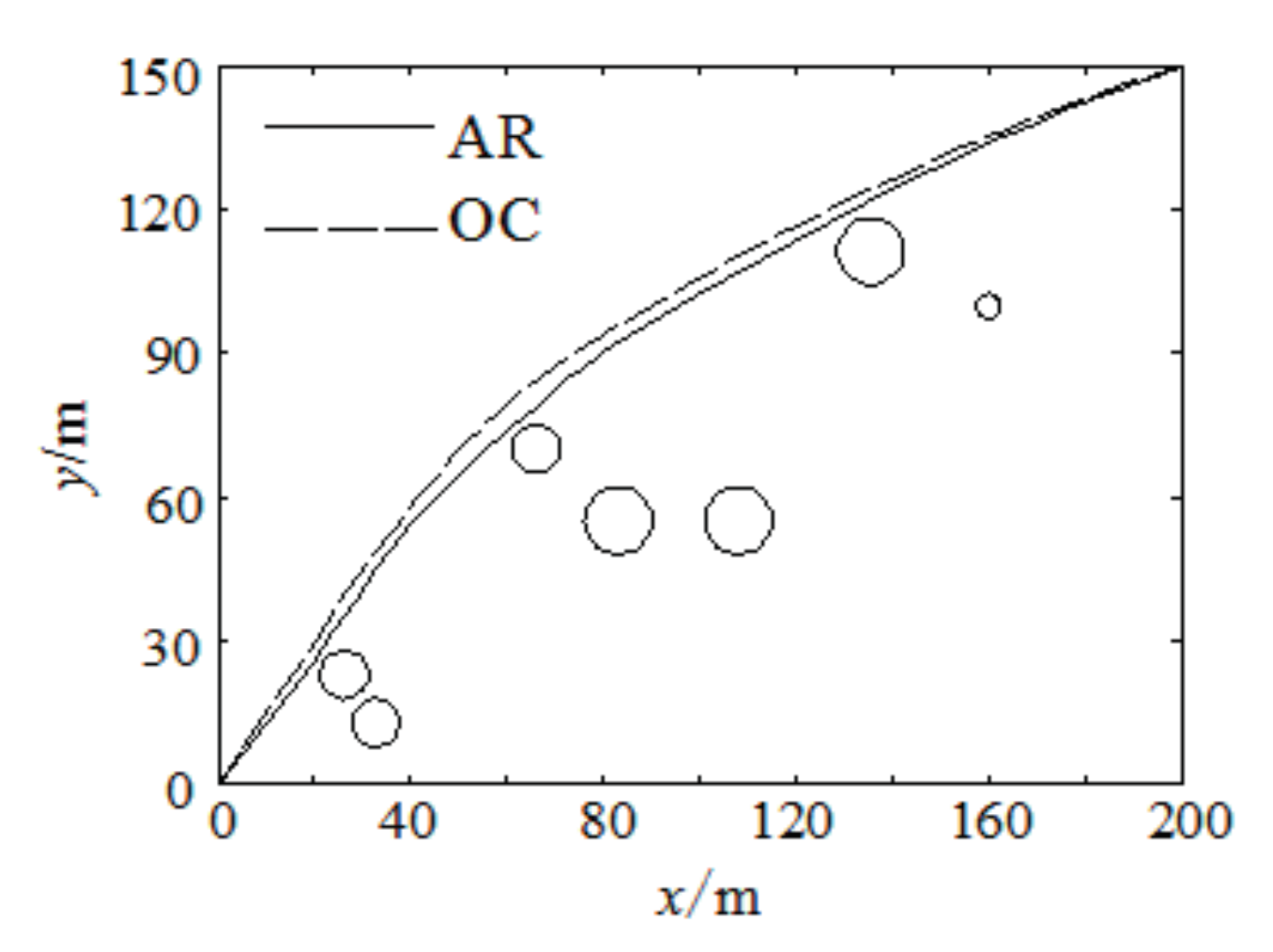
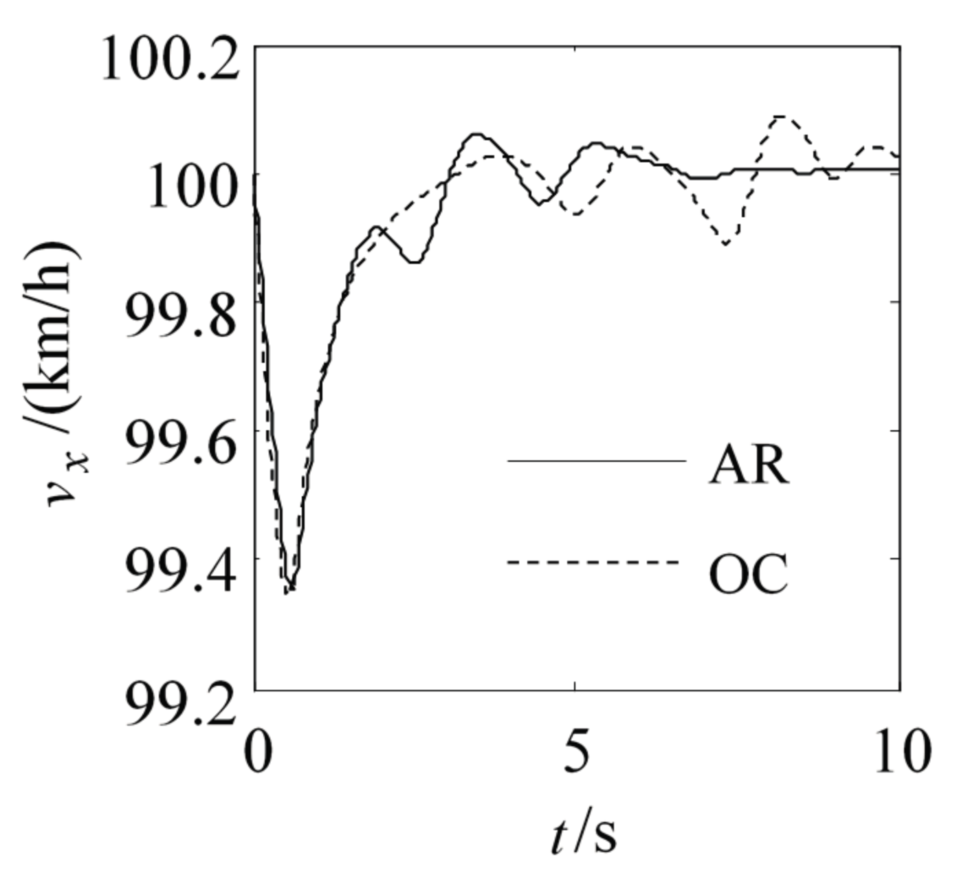
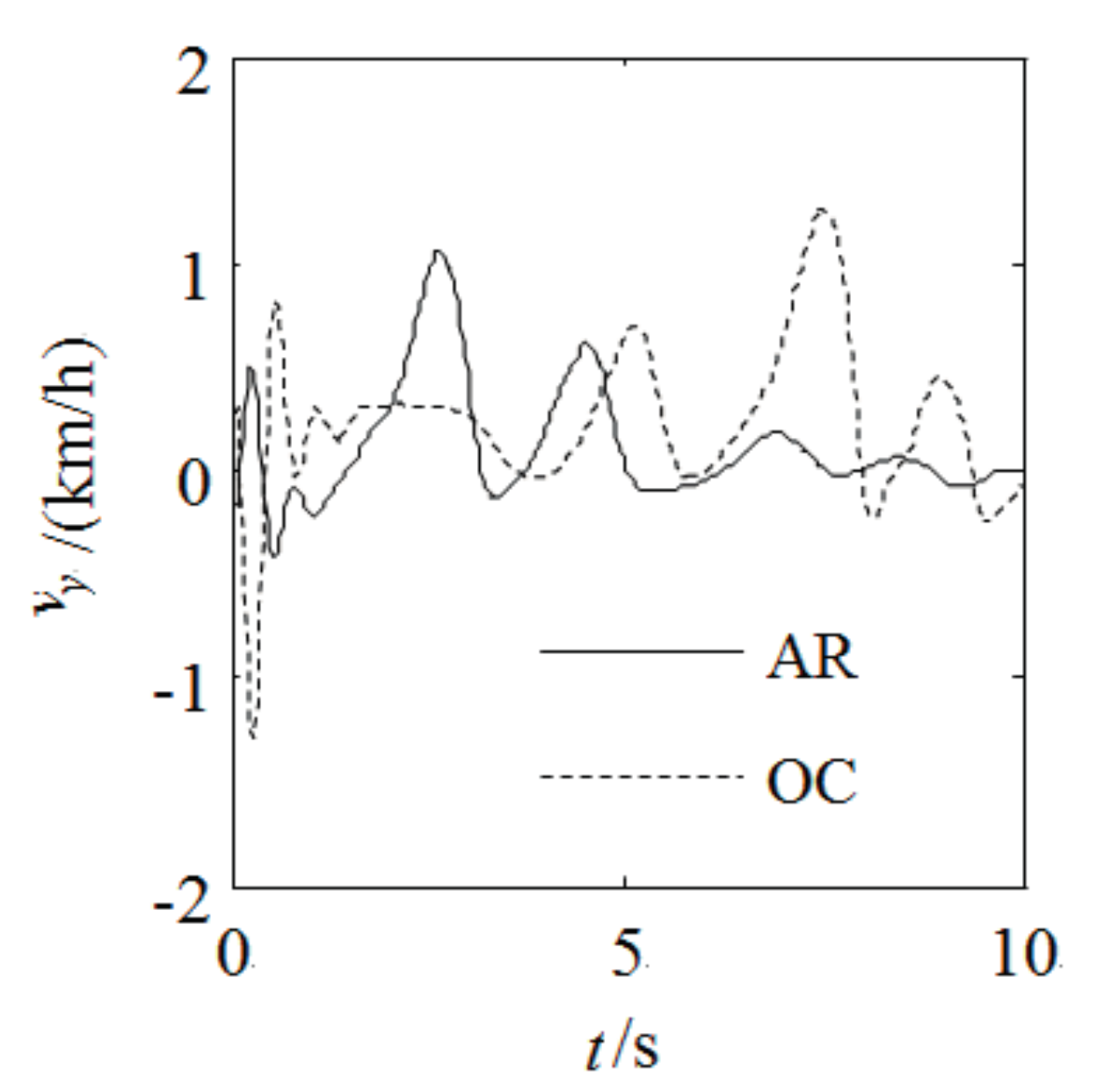
The one time iteration results are denoted as Da1 and Dz1, the iteration results generated from the weight set WDa0 generated by this paper’s method and WDz0 generated by the trajectory planning method of state space respectively. The finished weight adjusted results are denoted as Dan and Dzn respectively. From Figure 6, Figure 7, Figure 8, Figure 9 and Figure 10 are the trajectory and trajectory characteristic’s simulation results used this two methods respectively. We can see from Figure 6, Figure 7, Figure 8, Figure 9 and Figure 10 that the changed curves of the trajectory characteristic value optimized by AR are more smooth than the changed curves of the trajectory characteristic value optimized by OC, we also can see from Figure 10 that the lateral acceleration ay optimized by OC cannot meet the recognized driving stability constraint ay < 0.4 g, while the maximum lateral acceleration aymax = 0.39 g that is optimized by AR can meet the driving stability constraint ay < 0.4 g.
We can see from the two methods’ simulation results that when we need to plan the trajectory using the adverb constraint condition in the complex environment, the AR method is in well accordance with that of OC method, and that the AR is superior to OC for some parameters. Because of ACT-R’s human memory and learning ability, the trajectory planning method based on ACT-R can calculate the weight value more quickly and more close to the solution. The solution results returned by the solver have better convergence, it can better conform to the human’s behavioral characteristic and meet various constraint condition’s requirement. The simulation research shows that the AR method is applicable for high speed condition. The experiments with model car and comparison simulation research show that the AR method is feasible, and it can be deduced that the method could be applied for both low and high speed conditions.
6. The Experiment Verification of the Trajectory Planning Method
The experimental verification was done using the method of AR and obstacle avoidance path planning method based on fuzzy neural network fusion (abbreviation: FN) [30], respectively. The method of FN is a path planning method of combining with fuzzy and neural network, while the method AR is a trajectory planning method of combining with ACT-R and OC. The related configuration parameters for experimental vehicle: wheel base is 2.578 m, vehicle body length is 4.199 m, and vehicle body width is 1.786 m. This vehicle has been modified to be an intelligent vehicle, the vehicle can know the environmental information by CCD camera, by GPS, laser radar, and ultrasonic sensor installed on both sides of the vehicles for directional orientation. According to the real-time road information that is provided by the sensors, the methods of AR and FN is used to plan the trajectory and the trajectory is sent to steering controller, the controller will control the vehicle drive along the planned trajectory. The obstacles set {B} is as follows:
{B} = {[(755, 397), 50], [(630, 476), 50], [(490, 423), 25], [(185, 124), 50], [(251, 398), 50], [(290, 594), 50], [(782, 731), 25], [(550, 470), 50], [(436, 486), 50]}
The constraint set Re is as follows:
Re = {Hard = [ |ay max | ≤ 0.4 g]; Soft = [(safely), (better economy)]}
The soft constraints Soft = [(safely), (better economy)] can be expanded to{lower maximum velocity umax, lower average velocity uavg, lower maximum acceloration amax, The right distance dmin, the same as Soft = {40 km/h ≤ umax ≤ 60 km/h, 30 km/h ≤ uavg ≤ 50 km/h, amax ≤ 0.1 g, 3 m < dmin ≤ 4 m}.
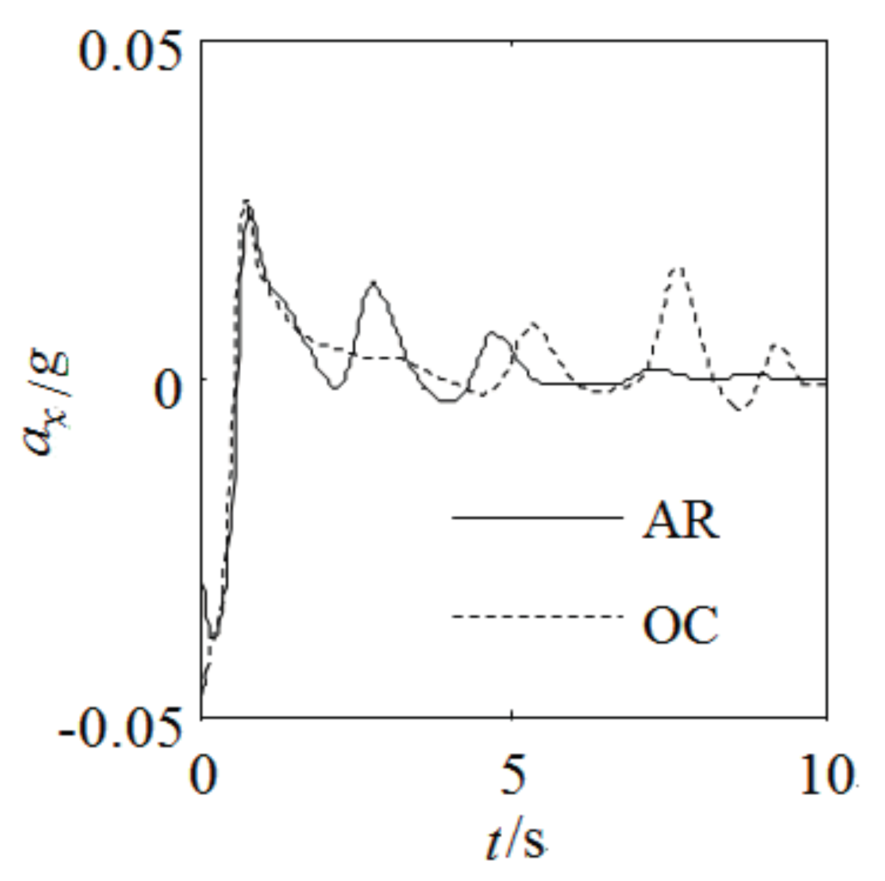
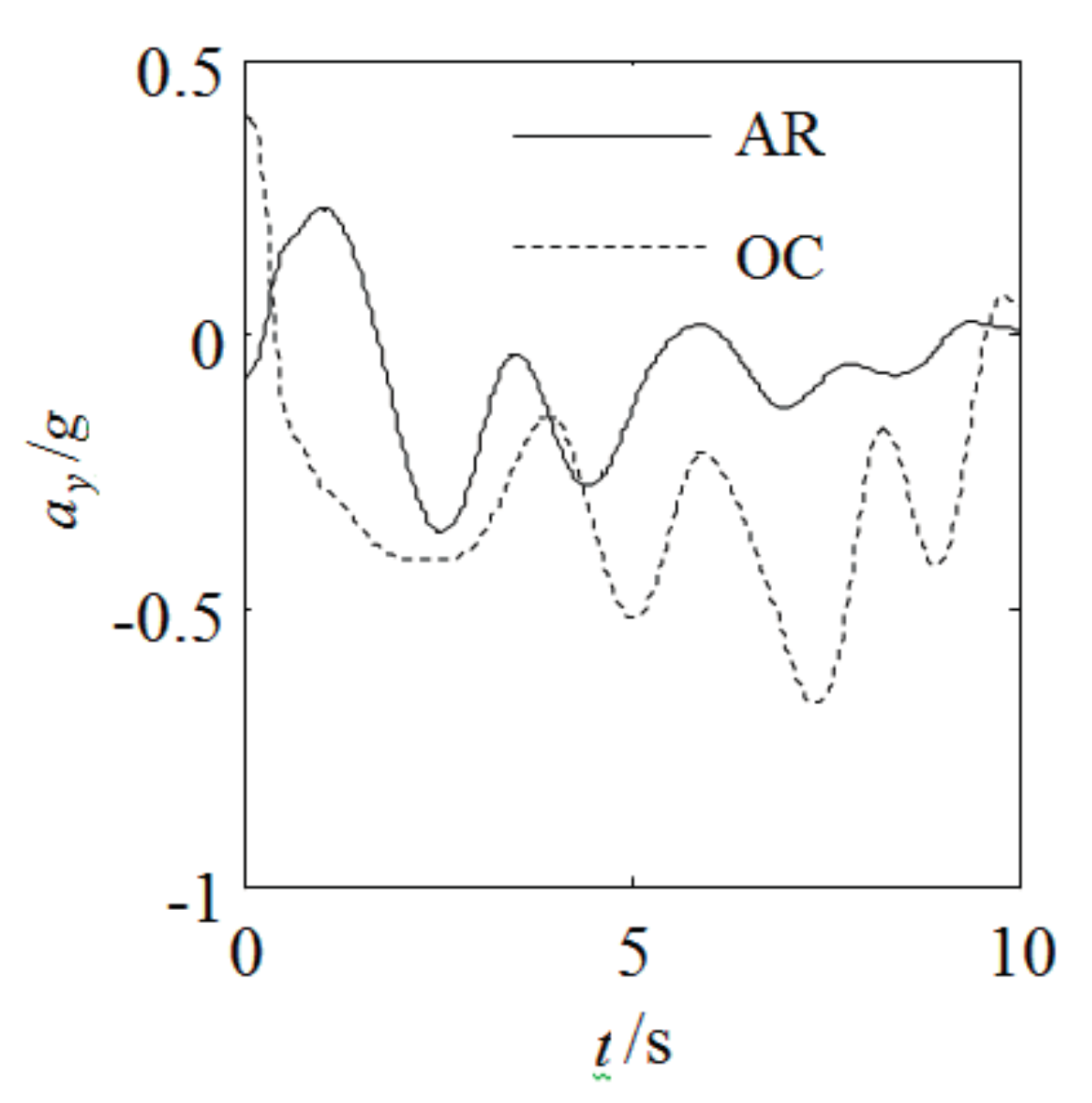
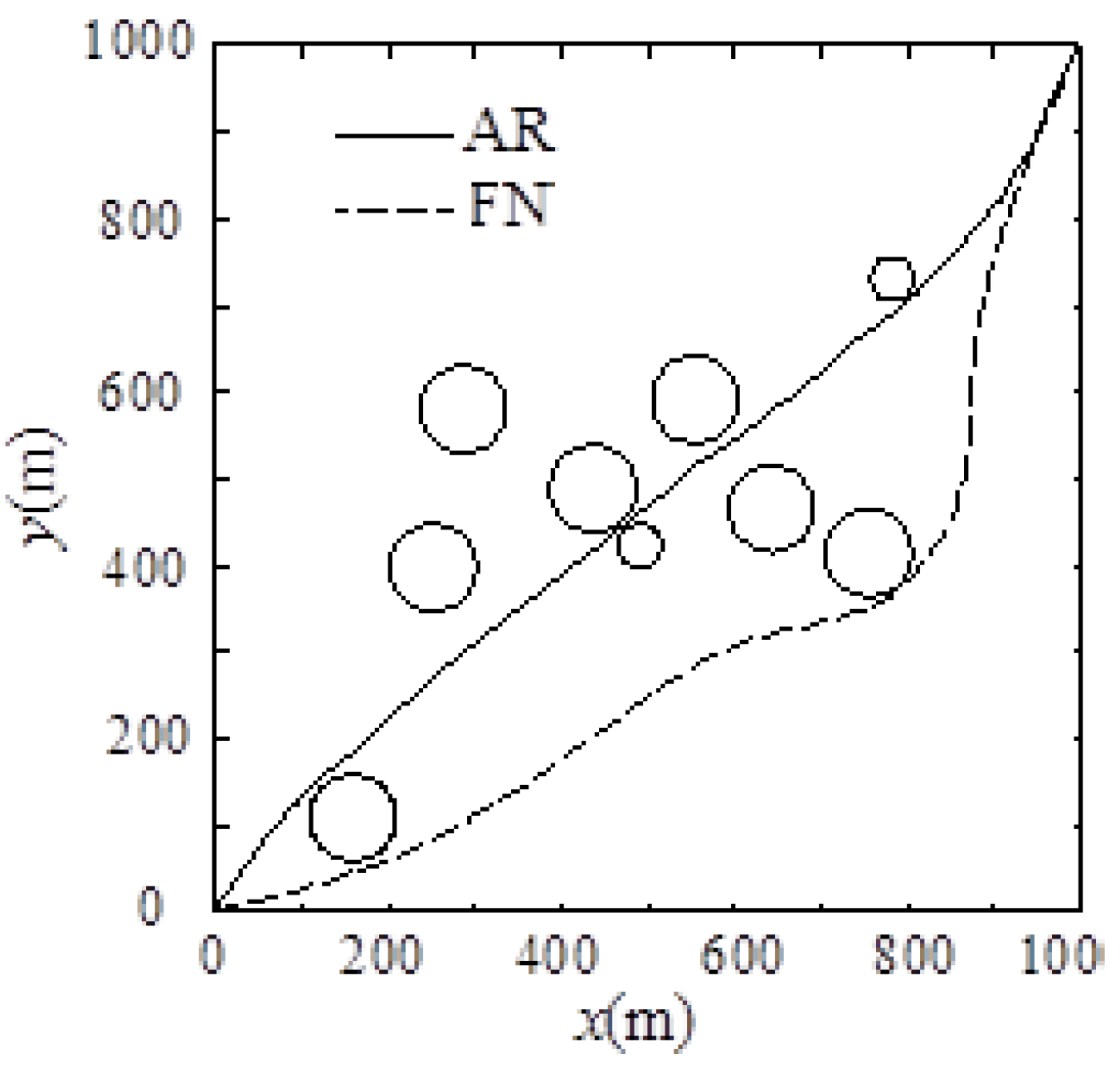
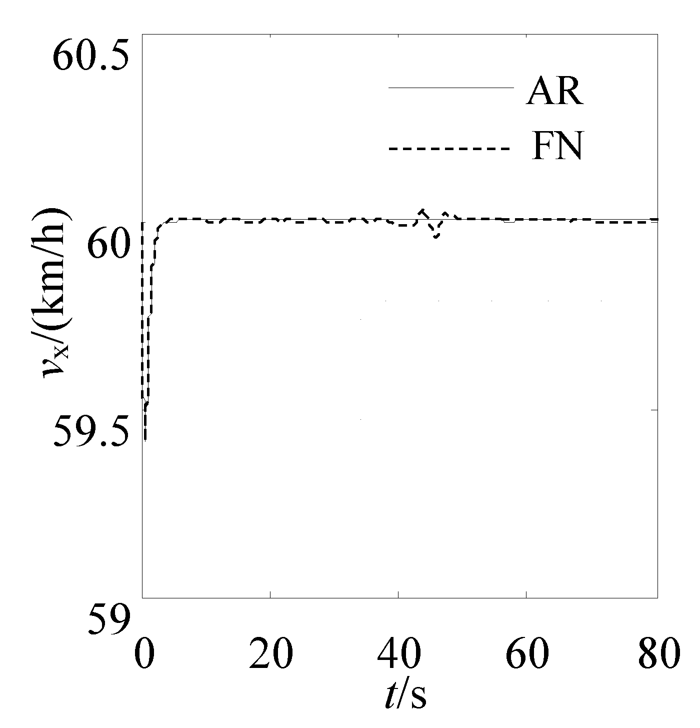
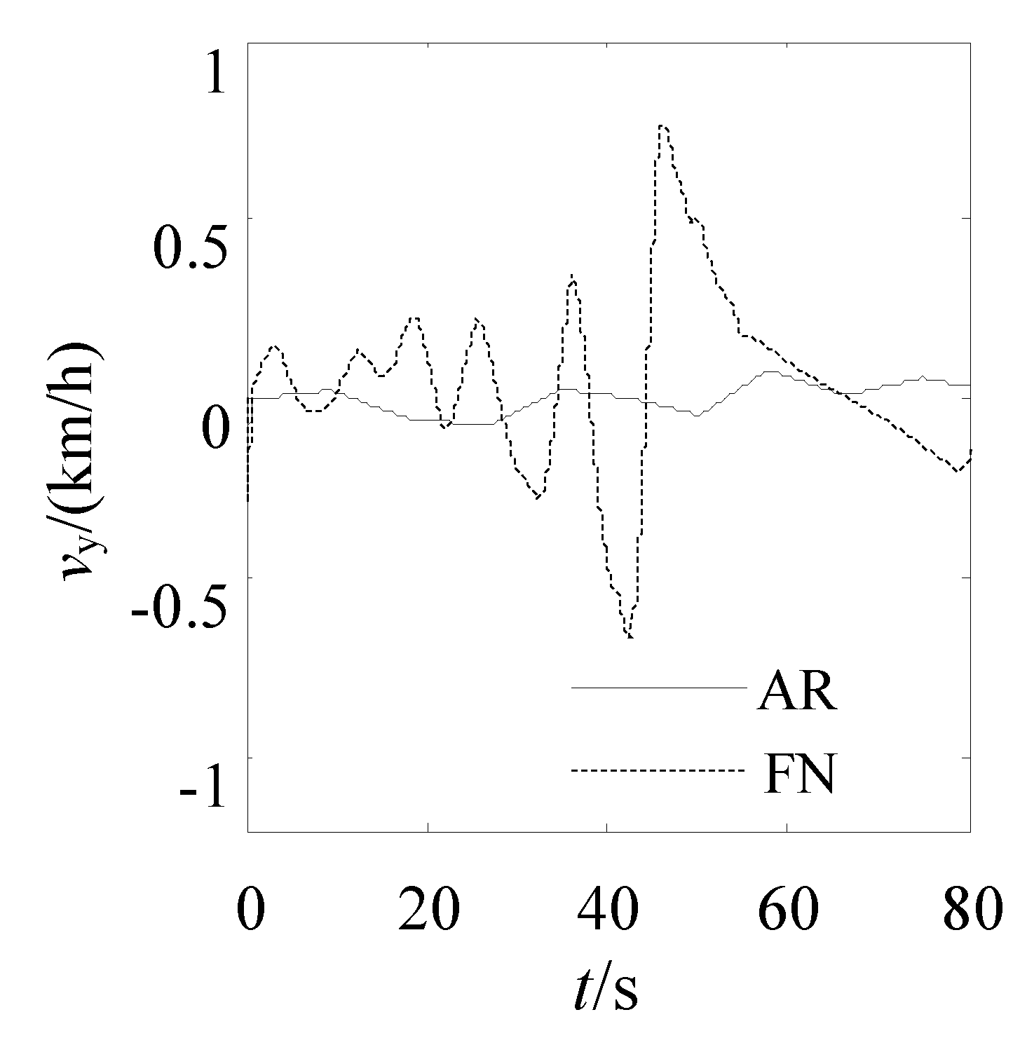
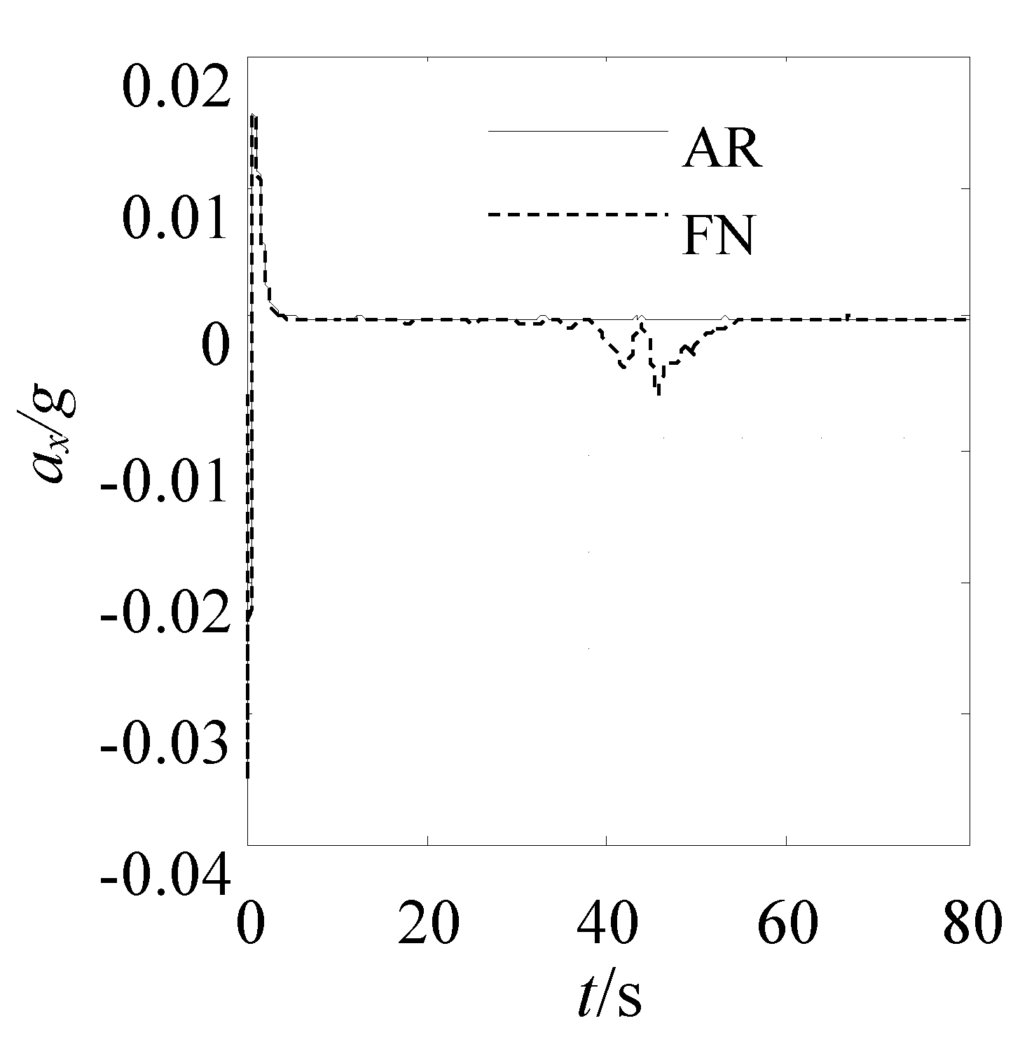
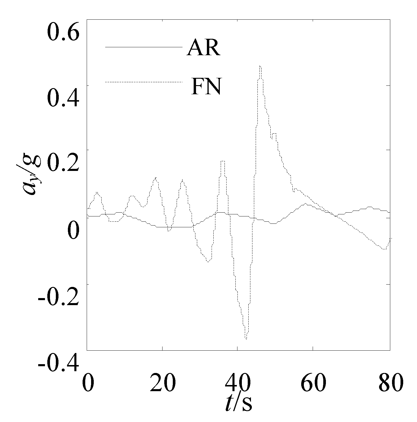
The vehicle’s driving trajectory planned by AR and FN is shown as Figure 11. We can see from Figure 11 that the shortest distance dmin = 3.6 m from the barrier that is planned by AR can meet the constraint condition 3 m < dmin ≤ 4 m, while the shortest distance dmin = 7.2 m from the barrier that is planned by FN cannot meet the constraint condition 3 m < dmin ≤ 4 m. The changed curve of the longitudinal velocity, lateral velocity, longitudinal acceleration, and lateral acceleration planned by AR and FN are shown as Figure 12, Figure 13, Figure 14 and Figure 15. We can see from Figure 12 that the maximum acceleration planned by AR is 0.123 g, it can satisfy the constraint condition ≤ 0.4 g, while the maximum acceleration planned by FN is 0.46 g, it cannot satisfy the constraint condition ≤ 0.4 g. We also can see from Figure 12, Figure 13, Figure 14 and Figure 15 that the variation curve of vehicle response parameters along the trajectory generated by AR is more smooth than that of vehicle response along the trajectory generated by FN, all of this indicated that the trajectory that is generated by AR can meet the dynamical constraint condition.
It can be obtained from the above analysis that the AR method is more feasible than the method FN. The method of FN is a path planning method, only the static path is planned in the method, however the trajectory parameters related time such as velocity and acceleration cannot be planned. So, when the vehicle driving along the planned path, the dynamical constraints may not be met. While the method AR is a trajectory planning method, not only the feasible path is generated, but also the trajectory parameters related to time, such as velocity and acceleration, can be planned. The time factor, vehicle model, human’s behavior characteristics and dynamical constraints are considered, so the planned trajectory generated by AR has more human behavior characteristics and meets the dynamical constraints. When the vehicle drives along the planned trajectory, the vehicle will not take side skidding and other problems that do not meet the driving stability.
7. Conclusions
This paper presents a new electric vehicle active obstacle avoidance system’s trajectory planning method based on ACT-R cognitive model, the conclusions are as follows.
- (1)
- This method contacts optimization control method and ACT-R cognitive model, the different driving trajectory can be dynamically planned to meet different constraints in different road environment.
- (2)
- The method based on the ACT-R cognitive model is mainly to intelligent optimization the trajectory’s parameters, the human’s behavioral characteristics is considered in the method, the planned trajectory has memory and learning ability and the trajectory’s parameters can be intelligent optimized to ensure the optimal trajectory’s generation.
- (3)
- The simulation analysis is done used this paper’s trajectory planning AR method and the method OC, respectively. The simulation results showed that AR method has obvious superiority than the OC method and the solution results returned by the solver have better convergence and can better conform to the human’s behavioral characteristic and can meet various constraint condition’s requirement. The simulation research showed that the AR method is applicable for high speed work condition.
- (4)
- The experimental verification was done used this paper’s trajectory planning method AR and the method FN, respectively. The experiment results showed that the AR method is more feasible then the FN method, the trajectory that was generated by AR has more human behavior characteristics and meets the dynamical constraints. When the vehicle travels along the planned trajectory, the vehicle will not take side skidding and other problems that do not meet the driving stability.
Acknowledgments
This project is supported by National Natural Science Foundation of China (Grant No. 51505258 and 51775268), Natural Science Foundation of Shandong Province, China (Grant No. ZR2015EL019), Science and technology development plan of Shandong Province, China (Grant No. 2013YD03059), Key Research and Development Project of Shandong Province, China (Grant No. 2016GNC112010), Agricultural Machinery and Equipment Research and Development Innovation Project of Shandong Province, China (Grant No. 2017YF013).
Author Contributions
Aijuan Li studied the trajectory planning method and wrote the paper; Wanzhong Zhao conceived and designed the experiments; Xuyun Qiu performed the experiments; Xibo Wang analyzed the data and modified the paper.
Conflicts of Interest
The authors declare no conflict of interest.
References
- Chen, C.; Xiong, R.; Shen, W. A lithium-ion battery-in-the-loop approach to test and validate multi-scale dual H infinity filters for state of charge and capacity estimation. IEEE Trans. Power Electron. 2018, 33, 332–342. [Google Scholar] [CrossRef]
- Xiong, R.; Cao, J.Y.; Yu, Q.Q. Reinforcement learning-based real-time power management for hybrid energy storage system in the plug-in hybrid electric vehicle. Appl. Energy 2018, 211, 538–548. [Google Scholar] [CrossRef]
- Wang, C.Y.; Zhao, W.Z.; Xu, Z.J.; Zhou, G. Path planning and stability control of collision avoidance system based on active front steering. Sci. China Technol. Sci. 2017, 60, 1231–1243. [Google Scholar] [CrossRef]
- Xiong, R.; Yu, Q.Q.; Wang, L.Y.; Lin, C. A novel method to obtain the open circuit voltage for the state of charge of lithium ion batteries in electric vehicles by using H infinity filter. Appl. Energy 2017, 207, 341–348. [Google Scholar] [CrossRef]
- Singh, A.; Singh, P.; Nishihara, O. Obstacle Avoidance by Steering and Braking with Minimum Total Vehicle Force. IFAC Pap. Online 2016, 49, 486–493. [Google Scholar] [CrossRef]
- Galvani, M.; Biral, F.; Nguyen, B.M.; Fujimoto, H. Four Wheel Optimal Autonomous Steering for Improving Safety in Emergency Collision Avoidance Manoeuvres. In Proceedings of the 2014 IEEE 13th International Workshop on Advanced Motion Control (AMC), Yokohama, Japan, 14–16 March 2014; pp. 362–367. [Google Scholar]
- Xiong, R.; Zhang, Y.; He, H.; Zhou, X.; Pecht, M. A double-scale, particle-filtering, energy state prediction algorithm for lithium-ion batteries. IEEE Trans. Ind. Electron. 2018, 65, 1526–1538. [Google Scholar] [CrossRef]
- Xiong, R.; Tian, J.P.; Mu, H.; Wang, C. A systematic model-based degradation behavior recognition and health monitor method of lithium-ion batteries. Appl. Energy 2017, 207, 367–378. [Google Scholar] [CrossRef]
- Zhao, L.; Sun, T.; Wang, J. Electronic Stability Control Based on Motor Driving and Braking Torque Distribution for a Four In-Wheel Motor Drive Electric Vehicle. IEEE Trans. Veh. Technol. 2016, 65, 4726–4739. [Google Scholar] [CrossRef]
- Lou, Y.; Feng, F.; Wang, M.Y. Trajectory Planning and Control of Parallel Manipulators. In Proceedings of the IEEE International Conference on Control and Automation, Christchurch, New Zealand, 9–11 December 2009; pp. 1013–1018. [Google Scholar]
- Goodarzi, A.; Esmailzadeh, E. Design of a VDC System for All-wheel Independent Drive Vehicles. IEEE Trans. Mech. 2007, 12, 632–639. [Google Scholar] [CrossRef]
- Liu, L.; Chen, C.; Zhao, X.; Li, Y. Smooth trajectory planning for a parallel manipulator with joint friction and jerk constraints. Int. J. Control Autom. Syst. 2016, 14, 1022–1036. [Google Scholar] [CrossRef]
- Li, X.; Sun, Z.; Cao, D.; He, Z.; Zhu, Q. Real-time trajectory planning for autonomous urban driving: Framework, Algorithms, and Verifications. IEEE/ASME Trans. Mechatron. 2016, 21, 740–753. [Google Scholar] [CrossRef]
- Li, X.; Sun, Z.; Cao, D.; Liu, D.; He, H. Development of a new integrated local trajectory planning and tracking control framework for autonomous ground vehicles. Mech. Syst. Signal Process. 2017, 87, 118–137. [Google Scholar] [CrossRef]
- González, D.; Pérez, J.; Milanés, V.; Nashashibi, F. A review of motion planning techniques for automated vehicles. IEEE Trans. Intell. Transp. Syst. 2016, 17, 1135–1145. [Google Scholar] [CrossRef]
- Zips, P.; Böck, M.; Kugi, A. Optimisation based path planning for car parking in narrow environments. Robot. Auton. Syst. 2016, 79, 1–11. [Google Scholar] [CrossRef]
- Jin, I.G.; Orosz, G. Optimal control of connected vehicle systems with communication delay and driver reaction time. IEEE Trans. Intell. Transp. Syst. 2016, 8, 2056–2070. [Google Scholar]
- Parhi, D.R.; Mohanty, P.K. IWO-based adaptive neuro-fuzzy controller for mobile robot navigation in cluttered environments. Int. J. Adv. Manuf. Technol. 2016, 83, 1607–1625. [Google Scholar] [CrossRef]
- Patle, B.K.; Parhi, D.; Jagadeesh, A.; Sahu, O.P. Real Time Navigation Approach for Mobile Robot. J. Comput. 2017, 12, 135–142. [Google Scholar]
- Trafton, J.G.; Hiatt, L.M.; Harrison, A.M.; Khemlani, S.S.; Schultz, A.C. Act-r/e: An embodied cognitive architecture for human-robot interaction. J. Hum.-Robot Interact. 2013, 2, 30–55. [Google Scholar] [CrossRef]
- Atashfeshan, N.; Razavi, H. Determination of the Proper Rest Time for a Cyclic Mental Task Using ACT-R Architecture. Hum. Factors 2017, 59, 299–313. [Google Scholar] [CrossRef] [PubMed]
- Pentecost, D.; Sennersten, C.; Ollington, R.; Lindley, C.; Kang, B. Using a physics engine in ACT-R to aid decision making. Int. J. Adv. Intell. Syst. 2016, 9, 298–309. [Google Scholar]
- Williams, J.R.; Jones, C.A.; Kiniry, J.R.; Spanel, D.A. The epic crop growth model. Trans. ASAE 1989, 32, 497–511. [Google Scholar] [CrossRef]
- Belavkin, R.V. On Emotion, Learning and Uncertainty: A Cognitive Modelling Approach. Ph.D. Thesis, The University of Nottingham, Nottingham, UK, 2003. [Google Scholar]
- Belavkin, R. Conflict Resolution by Random Estimated Costs. In Proceedings of the 17th European Simulation Multiconference, Nottingham, UK, 9–11 June 2013; pp. 105–110. [Google Scholar]
- Oh, H.; Jo, S.; Myung, R. Computational modeling of human performance in multiple monitor environments with ACT-R cognitive architecture. Int. J. Ind. Ergon. 2014, 44, 857–865. [Google Scholar] [CrossRef]
- Borst, J.P.; Anderson, J.R. A step-by-step tutorial on using the cognitive architecture ACT-R in combination with fMRI data. J. Math. Psychol. 2017, 76, 94–103. [Google Scholar] [CrossRef]
- Li, A.J.; Li, S.H.M.; Zhao, W.Z.; Shen, H.; Jiang, X.X. Optimal Control Theory Based Trajectory Generation Method Study for Intelligent Vehicle. J. Jilin Univ. (Eng. Technol. Ed.) 2014, 5, 1276–1282. [Google Scholar]
- Trafton, G.; Hiatt, L.; Harrison, A.; Tamborello, F.; Khemlani, S.; Schultz, A. ACT-R/E: An embodied cognitive architecture for inter action. J. Hum. Robot Interact. 2013, 2, 30–55. [Google Scholar] [CrossRef]
- Li, S.M.; Xin, J.H.; Shang, W.Y.; Huan, S.; Xiu, W. The Algorithm of Obstacle Avoidance Based on Improved Fuzzy Neural Networks Fusion for Exploration Vehicle. WSEAS Trans. Syst. Control 2009, 4, 140–150. [Google Scholar]
Figure 1.
The modular structure of ACT-R (Adaptive Control of Thought-Rational).

Figure 2.
The trajectory planning method’s framework structure based on ACT-R cognitive model.

Figure 3.
The flow chart of the trajectory planning method base on ACT-R.

Figure 4.
The initial weight WINT’s determination method flow chart.

Figure 5.
The estimation module’s flow chart.

Figure 6.
The sketch map of the vehicle’s driving trajectory optimized by AR and Optimal Control.

Figure 7.
The changed curve of the longitudinal velocity optimized by AR and OC.

Figure 8.
The changed curve of the lateral velocity optimized by AR and OC.

Figure 9.
The changed curve of the longitudinal acceleration optimized by AR and OC.

Figure 10.
The changed curve of the lateral acceleration optimized by AR and OC.

Figure 11.
The sketch map of the vehicle’s driving trajectory planned by AR and fuzzy neural network fusion (FN).
Figure 11.
The sketch map of the vehicle’s driving trajectory planned by AR and fuzzy neural network fusion (FN).

Figure 12.
The changed curve of the longitudinal velocity planned by AR and FN.

Figure 13.
The changed curve of the lateral velocity planned by AR and FN.

Figure 14.
The changed curve of the longitudinal acceleration planned by AR and FN.

Figure 15.
The changed curve of the lateral acceleration planned by AR and FN.


Table 1.
The trajectory characteristic’s descriptive knowledge of ACT-R weight adjustment model.
| Symbols | uavg (km/h) | umax (km/h) | amax (m/s2) | LIM (m) | dmin (m) | U (kg) | tf (s) |
|---|---|---|---|---|---|---|---|
| very low | [0, 15] | [0, 20] | [0, 0.05] | [0, 1] | [0, 1] | [0, 0.01] | [0, 1] |
| low | (15, 30] | (20, 40] | (0.05, 0.1] | (1, 2] | (1, 1.5] | (0.01, 0.1] | (1, 5] |
| lower | [30, 50] | [40, 60] | (0.1, 0.5] | (2, 3] | (1.5, 2] | (0.1, 0.5] | (5, 10] |
| medium | [50, 65] | [60, 80] | (0.5, 1] | (3, 4] | (2, 2.5] | (0.5, 1] | (10, 20] |
| higher | [65, 85] | [80, 100] | (1, 2] | (4, 5] | (2.5, 3] | (1, 2] | (20, 50] |
| high | [85, 100] | [100, 120] | (2, 3] | (5, 6] | (3, 4] | (2, 5] | (50, 100] |
| very high | [100, 160] | [120, 180] | [3, 10] | (6, 100] | (4, 50] | (5, 20] | (100, 1000] |
Table 2.
The procedural knowledge of ACT-R weight adjustment model.
| IF | THEN | |||||||
|---|---|---|---|---|---|---|---|---|
| Symbols | W3/W1 | uavg (km/h) | umax (km/h) | amax (m/s2) | LIM (m) | dmin (m) | U (kg) | tf (s) |
| very low | [0, 0.125] | [100, 160] | [120, 180] | [3, 10] | [0, 1] | [0, 1] | (5, 20] | [0, 1] |
| low | (0.125, 0.25] | [85, 100] | [100, 120] | (2, 3] | (1, 2] | (1, 1.5] | (2, 5] | (1, 5] |
| lower | (0.25, 0.5] | [65, 85] | [80, 100] | (1, 2] | (2, 3] | (1.5, 2] | (1, 2] | (5, 10] |
| medium | (0.5, 1] | [50, 65] | [60, 80] | (0.5, 1] | (3, 4] | (2, 2.5] | (0.5, 1] | (10, 20] |
| higher | (1, 2] | [30, 50] | [40, 60] | (0.1, 0.5] | (4, 5] | (2.5, 3] | (0.1, 0.5] | (20, 50] |
| high | (2, 4] | (15, 30] | (20, 40] | (0.05, 0.1] | (5, 6] | (3, 4] | (0.01, 0.1] | (50, 100] |
| very high | (4, 8] | [0, 15] | [0, 20] | [0, 0.05] | (6, 100] | (4, 50] | [0, 0.01] | (100, 1000] |
Table 3.
The procedural knowledge of ACT-R estimation module.
| IF | THEN |
|---|---|
| Ci meet constraints Rei | Return the right weigh set Wi |
| Ci cannot meet constraints Rei | Wi is the adjusted weight set Wi+1 |
| Wi+1 ∉ {PRi} | Return the right weight set Wi+1 |
| Wi+1 ∈ {PRi} | Return the wrong weight set Wi+1 |
Table 4.
The weight ratio’s descriptive knowledge of ACT-R weight adjustment model.
| Language Symbols | W3/W1 |
|---|---|
| very low | [0, 0.125] |
| low | (0.125, 0.25] |
| lower | (0.25, 0.5] |
| medium | (0.5, 1] |
| higher | (1, 2] |
| high | (2, 4] |
| very high | (4, 8] |
Table 5.
The weight adjusted result based on the state space trajectory planning method Optimal Control (OC).
Table 5.
The weight adjusted result based on the state space trajectory planning method Optimal Control (OC).
| Iterative Process | WDzi | umax (km/h) | uavg (km/h) |
|---|---|---|---|
| Dz0 | [1, 1, 1, 1] | 115.25 | 110.36 |
| Dz1 | [1, 1, 1.73, 1] | 108.66 | 105.81 |
| Dz2 | [1, 1, 1.73, 2.13] | 100.08 | 99.85 |
Table 6.
The weight adjusted result based on the ACT-R trajectory planning method AR.
| Iterative Process | WDai | umax (km/h) | uavg (km/h) |
|---|---|---|---|
| Da0 | [15, 3, 1, 1] | 105.78 | 103.85 |
| Da1 | [9.75, 1, 1, 1.27] | 100.07 | 99.76 |
© 2018 by the authors. Licensee MDPI, Basel, Switzerland. This article is an open access article distributed under the terms and conditions of the Creative Commons Attribution (CC BY) license (http://creativecommons.org/licenses/by/4.0/).
Share and Cite
MDPI and ACS Style
Li, A.; Zhao, W.; Wang, X.; Qiu, X. ACT-R Cognitive Model Based Trajectory Planning Method Study for Electric Vehicle’s Active Obstacle Avoidance System. Energies 2018, 11, 75. https://doi.org/10.3390/en11010075
AMA Style
Li A, Zhao W, Wang X, Qiu X. ACT-R Cognitive Model Based Trajectory Planning Method Study for Electric Vehicle’s Active Obstacle Avoidance System. Energies. 2018; 11(1):75. https://doi.org/10.3390/en11010075
Chicago/Turabian StyleLi, Aijuan, Wanzhong Zhao, Xibo Wang, and Xuyun Qiu. 2018. "ACT-R Cognitive Model Based Trajectory Planning Method Study for Electric Vehicle’s Active Obstacle Avoidance System" Energies 11, no. 1: 75. https://doi.org/10.3390/en11010075
Note that from the first issue of 2016, this journal uses article numbers instead of page numbers. See further details here.