Control of Two Satellites Relative Motion over the Packet Erasure Communication Channel with Limited Transmission Rate Based on Adaptive Coder

Abstract

The paper deals with the navigation data exchange between two satellites moving in a swarm. It is focused on the reduction of the inter-satellite demanded communication channel capacity taking into account the dynamics of the satellites relative motion and possible erasures in the channel navigation data. The feedback control law is designed ensuring the regulation of the relative satellites motion. The adaptive binary coding/decoding procedure for the satellites navigation data transmission over the limited capacity communication channel is proposed and studied for the cases of ideal and erasure channels. Results of the numerical study of the closed-loop system performance and accuracy of the data transmission algorithm on the communication channel bitrate and erasure probability are obtained by extensive simulations. It is shown that both data transmission error and regulation time depend approximately inversely proportionally on the communication rate. In addition the erasure of data in the channel with probability up to $0.3$ does not influence the regulation time for sufficiently high data transmission rate.

1. Introduction

In recent years, there has been a growing interest in using the differential force (i.e., the difference between the aerodynamic drag forces applied to the satellites) to eliminate the relative drift between the satellites in a swarm moving in a group (without the mandatory requirement to maintain relative position, cf. [1,2,3]). Various control algorithms using differential aerodynamic drag have been proposed in numerous publications, see [4,5,6,7,8,9,10,11,12,13,14,15,16]. One of the fundamental publications is the work by Leonard [17] where, based on the assumption of the possibility of changing the effective cross-section of satellites, a method of switching control has been developed. The differential force is created by changing the attack angles of the plates, located on the satellites, due to the rotation of the satellites with respect to the incident airflow. Kim et al. [18] deal with a satellite constellation, consisting of a leader satellite and surrounding slave ones. The orbit of the leader is considered as a reference, whilst the relative orbits of the followers are considered to be the Projected Circular Orbit (PCO), which is the relative orbit between the master and slave satellites, being a circular one when it is projected onto the local horizontal plane [19]. PCO predicted distances [20] between master and slave satellites are constant. The Hill–Clohessy–Witshire (HCW) equation describes the relative motion between the satellites in the local reference frame Local Vertical Local Horizontal (LVLH), with the origin on the master satellite. Monakhova and Ivanov [21] considered the problem of constructing a swarm from a large number of nanosatellites immediately after their separation from the launcher. To solve the problem of eliminating the drift between satellites, in [21] the decentralized control based on the force of aerodynamic drag is employed.

In the decentralized control of satellite formations, the problem of inter-satellite communication is very important. This communication is needed for navigation data exchange between the satellites. Particularly, Sarno et al. [22] presented innovative approaches for the guidance of spacecraft formations during reconfiguration. The method is conceived such that each satellite autonomously determines its tasks, allowing the algorithm to run faster, but entails a higher traffic on the inter-satellite communication link. Therefore the inter-satellite communication problem is a challenging one and attracts considerable interest of many researchers.

The electron density irregularities caused by ionosphering turbulence, scatterring radio waves, and affecting satellite communication were taken into account in [23]. Delay tolerant networking (DTN) protocols, such as bundle protocol and medium access control (MAC) were considered by Freimann et al. [24] as appropriate approaches for networks with intermittent connectivity such as deep space or low Earth orbit networks. A contact plan design approach was presented in [24] that solved the MAC problem by predicting additive multi-node interference and scheduling interference-free links based on these predictions. In [25], the algorithm called parallel data transmission for the navigation satellite network with agility link was proposed. Based on the network characteristics, the algorithm was designed with a polling pattern of link establishment and formulated as parallel data transmission problem based on deterministic scheduling the delay tolerant network. Cai et al. [26] presented a complete software-defined radio (SDR) model for inter-satellite communications and its implementation on a field-programmable gate array. The proposed SDR has low power consumption, which is suitable for power-limited small satellite systems. Davarian et al. [27] presented the results of a study exploring concepts for improving communications and tracking capabilities of deep space SmallSats. A detailed examination of relay proximity links and networks, where both proximity hardware and networking scenarios was addressed. A strategy for secure data correspondence between the smart city’s vehicular nodes, which uses the fundamentals of Elliptic Curve Cryptography (ECC) for key agreement and satellite communication for the transmission of messages over vehicles is proposed by Poomagal and Sathish Kumar [28]. Ujan et al. [29] presented a method to recognize received signal characteristics using a hierarchical classification in a multi-layer perceptron neural network. The experiments were described where a real-time video stream transmitted in the direct broadcast satellite was utilized with several modulation types of radio frequency interference. In [30], a routing algorithm to solve the link congestion problem caused by the limited topology in a topology-inhomogeneous Low Earth Orbit (LEO) satellite navigation augmentation network was proposed and a congestion avoidance routing model for the topology-inhomogeneous LEO satellite navigation augmentation network was established.

Important restrictions on the control performance are imposed by communication constraints. In [21], communication constraints were taken into account in the sense of the radio signal fading with increasing the inter-satellite distance. This leads to the space limitation within which the position of neighboring vehicles can be transmitted between them and, consequently, to reducing the number of satellites that are available for navigation data exchange. However the limitations on the transmission rate are not taken into account both in [21] and in the other above mentioned papers. It is worth noting that in practice the data transmission rate over the communication channels is always limited and, moreover, its minimization is highly useful from an energy consumption viewpoint. Among other things, decreasing the data transmission rate for the given power consumption can make it possible to increase the power of transmitted signals, expanding the area of inter-satellite interaction.

The present paper is focused on the reduction of the inter-satellite demanded communication channel capacity taking into account dynamics of the satellite’s relative motion and possibility of erasing the navigation data in the channel.

The limitations of control under constraints imposed by the limitations of the communication channel capacity, have been deeply studied within the control theoretic literature, see [31,32,33,34,35] and the references therein. A fundamental result establishing the smallest value for which the stabilization (estimation) problem for linear time invariant (LTI) systems is obtained by Nair and Evans [31] and presented in the form of the seminal Data Rate Theorem. However, the study of the application control problems in aerospace under communication constraints is still very limited.

In the present paper, a system of two coupled satellites is considered. As in [21], the satellites are assumed to be launched at the starting time in accordance to the specified separation conditions. It is assumed that the satellites move in a low circular near-Earth orbit and are controlled using the aerodynamic drag force, which is achieved by rotating the satellite relative to the incoming flow using a flywheel attitude control system. The main focus of the paper is in the navigation data exchange between the satellites to be used to keep the satellite motion in a swarm. To this end, the adaptive coding procedure is proposed and is studied for the cases of ideal and erasure communication channel. The regulation time is taken as the performance criterion, and its dependence on the data transmission rate is numerically studied.

The reminder of the paper is organized as follows. The existing results on control and estimation under information constraints are briefly recalled in Section 2, where the minimum necessary data rate for the estimation and control of Linear Time Invariant (LTI) systems in the form of the data rate theorem is specified and various coding/decoding schemes are described. Section 3 is devoted to the dynamics of two satellites’ relative motion in a near-circular orbit. The main result is concentrated in Section 4. This section starts with designing the control law, which ensures the asymptotic regulation of the satellites relative motion (Section 4.1). The design is based on the linearized dynamics model without taking into account the control signal saturation. The classical modal control approach based on the pole-placement technique is employed [36]. The behavior of the system with the saturation in control is studied in the subsequent sections by the simulations. The next stages of the present study are dedicated to the evaluation of the proposed scheme of the inter-satellites data transmission over a digital communication channel, aimed for reducing the necessary channel capacity. To this end, the adaptive coding procedure for the position transmission between the satellites in the formation, employing the kinematics process description, is introduced in Section 4.2. It is worth mentioning that the application of this procedure makes it possible to avoid measuring the time derivatives of the satellites relative position (these derivatives are needed for control) due to the state observer, which is embedded into the adaptive coder/decoder pair. Then in Section 4.3, the model of the erasure communication channel, adopted in the present research, is described. Results of the numerical study of the closed-loop system performance and accuracy of the data transmission algorithm dependence on the communication channel bitrate and erasure probability obtained based on the extensive simulations are presented in Section 4.4. Concluding remarks and the future work intentions given in Section 5 finalize the paper.

2. Control and Estimation under Information Constraints

2.1. Problem Description

Let us consider control and observation (estimation) systems containing a digital communication channel. For these systems, plant output measured by the sensor at discrete instants $t_k=k{T}_0$, where $T_0$ denotes the sampling interval, $k=0,1,\dots$, is converted by the coder into the characters of the coding alphabet $\mathbb{S}$. The sequence of characters is transmitted over a digital communication channel to the decoder. The decoder transforms messages from the transmitted form in a form adequate to subsequent calculations and transformations by the controller. In [37,38,39] the communication channel was considered of limited capacity, but was otherwise ideal. The cases of packet erasure channel and ‘blinking’ channel widely appear in various real-world systems, see, e.g., [40,41,42,43,44,45,46,47,48,49]. Therefore, for a more realistic analysis, the properties of the communication channel, such as distortion, erasure, and data loss, should be taken into account. In the present study, the effect of data erasure is considered.

Signal quantization introduces essentially non-linear properties into the system, characterized by the presence of the dead zone, discontinuities, and saturation (associated with bit grid overflow). Additionally, the signal sampling on time involves the hybrid (continuous-discrete) system description. A rigorous examination of the influence of time sampling and the level quantization is a complex nonlinear analysis problem, that usually does not have an exact analytical solution. In the early studies, the level quantization in digital control systems was usually considered a source of independent additive random noise affecting the system. This assumption makes it possible to significantly simplify the study of level quantized systems, especially for LTI plants. However, if the quantization level is relatively high (for example, in the case of binary quantization), this can lead to the emergence of self-oscillations and even the system divergence, see [50,51,52,53]. Therefore, to analyze the system, its nonlinear model is required. Besides, the possibility of the bit grid overflow can also affect the quantizer, as a result of which the saturation is introduced to the control loop [54,55].

2.2. Minimum Necessary Data Rate for Estimation and Control

The limitation of the data transmission rate over the communication channel can be expressed in informational terms. Assume that coding alphabet $\mathbb{S}$ consists of $\mu$ elements. Then at each step $k=0,1,\dots$ over the channel an amount of $\tilde{R}={log}_2\mu$ bit can be transmitted per each step. Let the data transmission be carried out at discrete instants $t_k=k{T}_0$, where $T_0$ is the sampling interval. Then the data transmission rate in bits per second is as $R=T_0^{-1}{log}_2\mu$ bit/s. In this regard, one speaks of “information constraints” in control and estimation problems.

The problem of determining the minimum bandwidth of the communication channel, at which it is possible to provide the required estimation accuracy, is posed and partially solved by Nair and Evans [56]. The sufficient condition for the value obtained in Nair and Evans [56] was developed in subsequent works in the form of the Data Rate Theorem which is a fundamental result establishing the smallest value for which the stabilization (estimation) problem for linear systems is solvable in principle. Nair and Evans [31] studied the exponential stabilizability of LTI plants in the sense of achieving an exponential moment stability. For a deterministic initial state case the result of [31] can be roughly presented in the following form [57].

Let the LTI discrete-time plant be described by the difference equation:

$$\begin{array}{c}\hfill x[k+1]=Ax\left[k\right]+Bu\left[k\right],y\left[k\right]=Cx\left[k\right],k=0,1,\dots \end{array}$$

(1)

where $x\left[k\right]\in {\mathbb{R}}^n$, $y\left[k\right]\in {\mathbb{R}}^l$, and $u\left[k\right]\in {\mathbb{R}}^m$ are the state, output, and control vectors, respectively; A, B, and C are the matrices of the corresponding dimensions; and $k\in {\mathbb{Z}}_{+}$ denotes the step number (the discrete time). It is assumed that pair $(A,B)$ is reachable and $(C,A)$ is observable. Let the sensor be connected to the controller over a digital communication channel, and no more than $\tilde{R}$ bits of data can be transmitted at each step k. Then the necessary and sufficient conditions for $\rho$-exponential (with the prespecified stability bound $\rho >0$) stabilization are given by the inequality [31]:

$$\begin{array}{c}\hfill \tilde{R}>\sum _{{\eta }_j\ge \rho }{log}_2\left|{\displaystyle \frac{{\eta }_j}{\rho }}\right|(\mathrm{bit}\mathrm{per}\mathrm{step}),\end{array}$$

(2)

where ${\eta }_j$ are the eigenvalues of matrix A, $j=1,\dots ,n$. The right-hand side of (2), denoted as ${\tilde{R}}_{NE}={\displaystyle \sum _{{\eta }_j\ge \rho }}{log}_2\left|{\displaystyle \frac{{\eta }_j}{\rho }}\right|$ (the Nair–Evans-, or NE-number), gives a tight admissible bound when $\rho$-exponential stabilization can be achieved. For real-time systems with the constant sampling interval $T_0$, NE-number $R_{NE}$ in bits per second has a form:

$$\begin{array}{c}\hfill R_{NE}={\displaystyle \frac{1}{T_0}}{\tilde{R}}_{NE}={\displaystyle \frac{1}{T_0}}\sum _{{\eta }_j\ge \rho }{log}_2\left|{\displaystyle \frac{{\eta }_j}{\rho }}\right|(\mathrm{bit}\mathrm{per}\sec \mathrm{ond}).\end{array}$$

(3)

Extensions of this result for stabilizing nonlinear systems in the vicinity of the origin and observing nonlinear systems through finite capacity communication channels, including large networks, were obtained in the series of the subsequent papers, see [58,59,60,61,62] to mention a few.

It is worth mentioning that on practice, the data transmission rate can not be taken as small as the NE-number (3) gives due to several reasons for the data bitrate being usually much greater than $R_{NE}$, but the NE-number can serve as a measure showing the maximum available possibilities of estimation and control over the existing communication channel. Furthermore, a promising approach is to employ the event-triggered control instead of the control with constant sampling time, see e.g., [63,64,65].

2.3. Coding/Decoding Schemes

Under the assumption that the sampling time $T_0$ can be chosen arbitrarily, optimality of the binary coding in the sense of the required transmission rate (in bit-per-second) has been proven in [39], see also [66]. Therefore in the present study the binary quantizer is used as a core element for the coding procedure.

2.3.1. Static Binary Quantizer

Let $\sigma \left[k\right]$ be a scalar information signal to be transmitted over the digital communication channel in discrete instants $t_k=k{T}_0$, where $k=0,1,\cdots \in {\mathbb{Z}}_{+}$ is a sequence of natural numbers, and $T_0$ is the sampling interval. Let us introduce the following static quantizer:

$$\begin{array}{c}\hfill q(\sigma ,M)=M\left[k\right]s,s=sign\left(\sigma \right),\end{array}$$

(4)

where $sign(·)$ is the signum function: $sign\left(\sigma \right)=1$, if $\sigma \ge 0$, $sign\left(\sigma \right)=-1$, if $\sigma <0$. Parameter M is referred to as a quantizer range. The output signal of the quantizer is represented as one-bit information symbol from the coding alphabet $\mathcal{S}=\{-1,1\}$, and is transmitted to the decoder. Note that for the binary coder, the transmission rate is as $R=1/T_0$ bit per second. It is assumed that the equi-memory condition is fulfilled, i.e., the coder and decoder make decisions based on the same information [67,68]. The binary output codeword $s\in \mathcal{S}$ is transmitted to the decoder.

2.3.2. Zooming Strategies

In time-varying quantizers [33,39,69,70,71,72] range M is updated with time. Using such a zooming strategy improves the steady-state accuracy of the transmission procedure and at the same time prevents the encoder saturation at the process beginning. The values of $M\left[k\right]$ can be precomputed (the time-based zooming) [39,73,74], or current quantized measurements can be used at each step for updating $M\left[k\right]$ (the event-based zooming). For an audio channel, Moreno-Alvarado et al. [75] developed the coding schemes with the capacity to simultaneously encrypt and compress audio signals, which makes possible increasing necessity for transmitting sensitive audio information over insecure communication channels.

The event-based zooming can be realized in the form of the adaptive zooming [76,77,78,79], where the quantizer’s range is adjusted automatically depending on the current variations of the transmitted signal.

For the binary quantizer the following adaptive zooming algorithm was proposed and experimentally studied in [78]:

$$\begin{array}{c}\hfill \begin{array}{c}\lambda \left[k\right]=\left(s\right[k]+s[k-1]+s[k-3\left]\right)/3,s[-1]=s[-2]=0,\hfill \\ \\ M[k+1]=m_c+\left\{\begin{array}{cc}\rho M\left[k\right],\hfill & \mathrm{if}\left|\lambda \right[k\left]\right|\le 0.5,\hfill \\ M\left[k\right]/\rho ,\hfill & \mathrm{else},\hfill \end{array}\right.\hfill \\ \overline{\sigma }\left[k\right]=M\left[k\right]s\left[k\right],\hfill \end{array}\end{array}$$

(5)

where $M\left[0\right]=M_0$ is an initial value of $M\left[k\right]$ (the design parameter) and $\overline{\sigma }\left[k\right]$ denotes the value of $\sigma \left[k\right]$ recovered at the decoder side from binary values $s\left[k\right]$. Unlike the case of the time-based zooming, the initial value $M_0$ can be chosen arbitrarily, since $M\left[k\right]$ is automatically adjusted and can be increased or decreased during the zoom-in or zoom-out stages.

2.3.3. Coders with Memory

The coding/decoding procedure can include the embedded observer, which adds a memory to the coder. The following model of drive process is used:

$$\begin{array}{cc}& \dot{x}\left(t\right)=Ax\left(t\right)+B\phi \left(t\right),y\left(t\right)=Cx\left(t\right),x\left(0\right)=x_0\end{array}$$

(6)

where $x\left(t\right)\in {\mathbb{R}}^n$ is the process state space vector; $y\left(t\right)$ is the scalar measured signal; $A\in {\mathbb{R}}^{n\begin{array}{c}\times \end{array}n}$, $B\in {\mathbb{R}}^{n\begin{array}{c}\times \end{array}1}$ are given real matrices; and $\phi \left(t\right)$ is the external input signal which is assumed to be the same both on the transmitter and the receiver sides (so that the equi-memory condition be fulfilled).

The quantized observation error $\overline{\sigma }\left[k\right]$ is defined as a deviation between measured signal $y\left(t\right)$ and its estimate $\widehat{y}\left(t\right)$ quantized with given $M\left[k\right]$ as follows:

$$\begin{array}{c}\hfill \overline{\sigma }\left[k\right]=q\left(y\left(t_k\right)-\widehat{y}\left(t_k\right),M\left[k\right]\right),t_k=k{T}_0.\end{array}$$

(7)

where the estimate $\widehat{y}\left(t\right)$ is generated by the following observer:

$$\begin{array}{c}\hfill \dot{\widehat{x}}\left(t\right)=A\widehat{x}\left(t\right)+B\phi \left(\widehat{y}\left(t\right)\right)+L\overline{\sigma }\left(t\right),\widehat{y}\left(t\right)=C\widehat{x}\left(t\right),\end{array}$$

(8)

where $\widehat{x}\left(t\right)\in {\mathbb{R}}^n$ is the state estimation vector; $\widehat{y}\left(t\right)$ is the estimate of the drive process; L is $\left(n\begin{array}{c}\times \end{array}1\right)$-matrix (the column-vector) of the observer parameters; and the continuous-time observation error $\overline{\sigma }\left(t\right)$ is found as an extension of $\overline{\sigma }\left[k\right]$ over the sampling interval. In the case of the zero-order extrapolation, $\overline{\sigma }\left(t\right)$ has a form $\overline{\sigma }\left(t\right)=\overline{\sigma }\left[k\right]$ as $t_k\le t<t_{k+1}$.

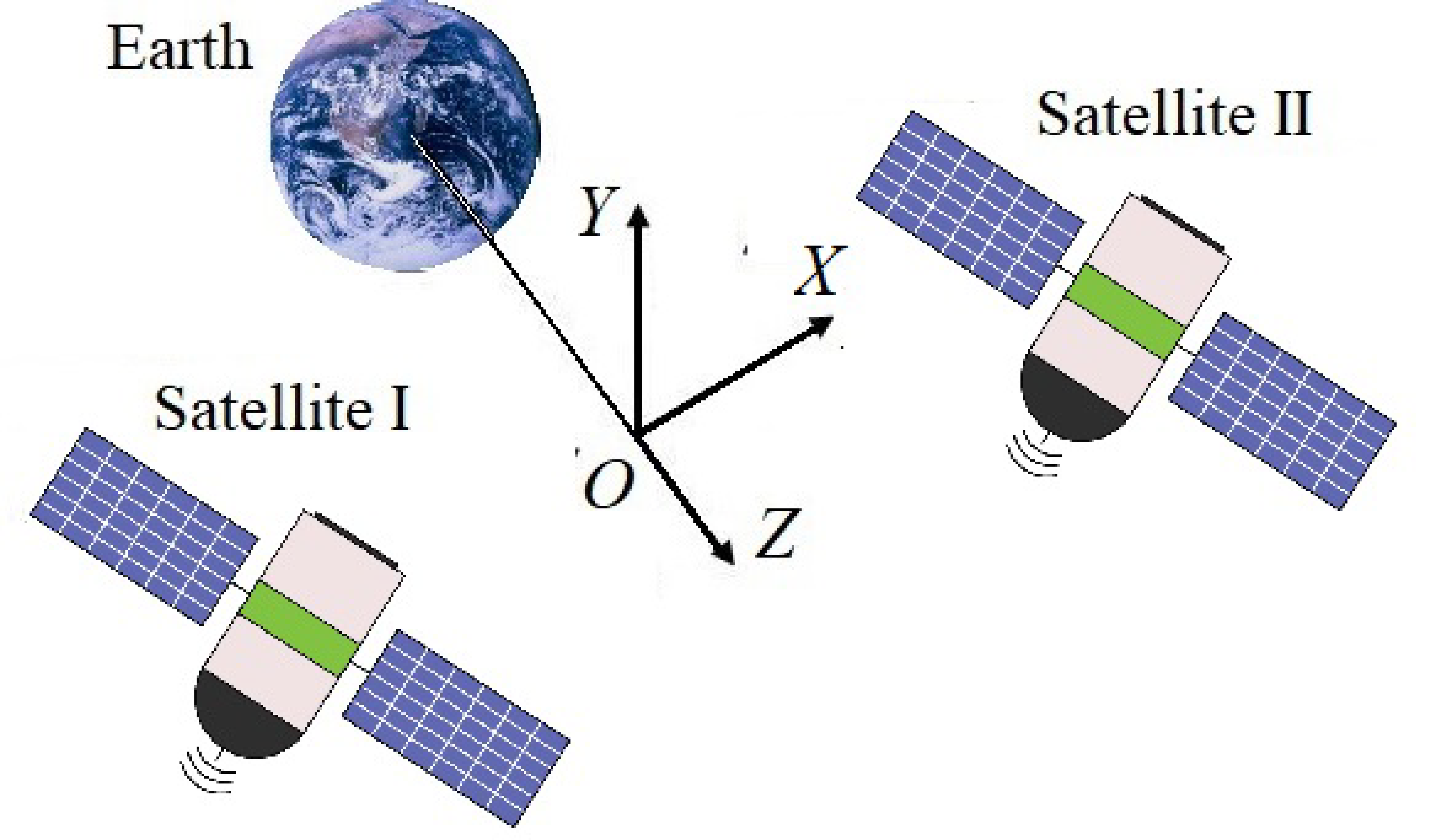
3. Relative Motion Dynamics of Two Satellites in a Near-Circular Orbit

For describing the dynamics of the relative motion of two satellites, moving in near-circular orbits at the Earth’s central gravitational field, equations in the Local Vertical Local Horizontal (LVLH) reference system in relative coordinates according to the HCW model is used, see [21,80,81,82,83,84].

In the present paper, the LVLH reference system is employed, where the OZ axis is directed from the center of the Earth, the OY axis is directed normal to the orbital plane, and the OX axis complements the triple to the right coordinate frame, see Figure 1.

Taking into account that the motion along the normal to the orbital plane (along OY axis) is isolated, and proceeding from the universal gravitation law and Kepler’s third law under the assumption that for distance $\rho$ of the satellite to the center of the Earth inequalities $\rho \gg x,z$ are held, one obtains the following HCW equations of satellite motion in the LVLH local coordinate system:

$$\begin{array}{cc}\hfill & \ddot{x}=-2\omega \dot{z}+F_x,\hfill \end{array}$$

(9)

$$\begin{array}{cc}\hfill & \ddot{z}=2\omega \dot{x}+3\omega z+F_z,\hfill \end{array}$$

(10)

where $F_x$, $F_z$ are the components of the vector of non-gravitational forces applied to the satellite, expressed in acceleration units. These forces include the aerodynamic drag force $f_x$ along the OX axis, which is controlled by the satellite turning through the attack angle $\alpha$. Based on the physical considerations it is valid that $f_x=f_x\left(\alpha \right)\le 0$, $f_x\left(0\right)\le \left|f_x\right|\le f_x(\pi /2)$. Therefore it is natural considering angle $\alpha$ within $0\le \alpha \le \pi /2$. In (10)$,\omega$ denotes the averaged angular velocity of the spacecraft in orbit and satisfies the expression $\omega =\sqrt{\mu /a^3}$ where $\mu =GM$, G is the gravitational constant, M is the mass of the central body (for the Earth, $\mu =$398,603$\begin{array}{c}\times \end{array}{10}^9{\mathrm{m}}^3{\mathrm{s}}^{-2}$), and a is the semi-major axis of the satellite orbit. HCW Equations (9) and (10) are derived under the assumptions: $\sqrt{x^2+z^2}$ is small compared to $\rho$; the aerodynamic force is small, the acceleration caused by it does not exceed $1.7\begin{array}{c}\times \end{array}{10}^{-6}$ m/s${}^2$; the eccentricity of the orbit is small, the orbit is very close to the circular one; and the orbital rate $\omega$ is approximately constant. For the resulting system (9), (10) in [17], a non-degenerate coordinate transformation is performed to the real Jordan form [36], as a result of which the model (9), (10) is represented in the form of a double integrator and a harmonic oscillator, connected in parallel. For the double integrator, a speed-optimal control is created in the form of relay feedback with a quadratic switching function. A similar, but technically more complex approach is used for the harmonic oscillator. Since the control is scalar, it is not possible to apply both control laws simultaneously and independently to both the double integrator and oscillator. To resolve this contradiction, Leonard [17] developed and studied for different flight scenarios an algorithm for switching from one control law to another, based on the specifics of the rendezvous problem requirements. The linearized equations of the satellites relative motion in the OXZ plane (9), (10) in the state-space form read as (cf. [5,21]):

$$\begin{array}{cc}\hfill & \dot{\chi }=A\chi +Bu,y=C\chi ,\hfill \end{array}$$

(11)

$$\begin{array}{cc}\hfill & u=-\phi \left(y\right),\hfill \end{array}$$

(12)

where $\chi ={\left[\begin{array}{cccc}\hfill x_{12}& {\dot{x}}_{12}& z_{12}\hfill & {\dot{z}}_{12}\end{array}\right]}^{\mathrm{T}}\in {\mathbb{R}}^4$ is the system state vector, where $x_{12}$ denotes the difference in coordinates of the second and first satellites along the OX axis, $x_{12}=x_2-x_1$; $z_{12}=z_2-z_1$; and u denotes the control action (difference of aerodynamic forces acting on satellites, in units of acceleration). It is limited in modulus by the value $u_{\max }$. Equation (12) closes the feedback loop. In it, y is the output of the linear controller in the feedback, $\phi (·)$ is a nonlinear function describing the limitation of the control action, which is assumed to be the saturation function, $\phi \left(y\right)={sat}_{u_{\max }}\left(y\right)$. Since for each satellite the aerodynamic drag force is negative (that is, it acts against the direction of motion along the longitudinal axis and lies in the interval $[-u_{\max },0]$), then in order to provide the desired differential control $-u_{\max }\le u_{ij}\le u_{\max }$, the actual steering (braking) action should only be applied to the first (along X-axis) satellite of the pair, see [21].

Matrices of dynamics model (11) have the form:

$$\begin{array}{cc}\hfill & A=\left[\begin{array}{cccc}0& 1& 0& 0\\ 0& 0& 0& -2\omega \\ 0& 0& 0& 1\\ 0& 2\omega & 3{\omega }^2& 0\end{array}\right],B=\left[\begin{array}{c}0\\ 1\\ 0\\ 0\end{array}\right]\hfill \\ \hfill & K=\left[\begin{array}{cccc}{k}_1& k_2& k_3& k_4\end{array}\right],\hfill \end{array}$$

(13)

Coefficients $k_i$, $i=1,\dots ,4$ are chosen at the stage of the control law synthesis.

4. Main Result

4.1. Control Law Design

Suppose that each satellite has the onboard navigation equipment, e.g., the GLONASS/GPS receivers [85], for determining its position and is able to share this information via the digital inter-satellite communication channel. Therefore it is assumed that the onboard control system of each satellite is supplied by the values of all the relative coordinates $x_{12}=x_2-x_1$, $z_{12}=z_2-z_1$ and their time derivatives. Control signals for each satellite are generated so as to provide the difference $u=u_2-u_1$, generated in accordance with the chosen control law $u=U(x_{12},z_{12},{\dot{x}}_{12},{\dot{z}}_{12})$. In the present study, for control law design the pole-placement technique is employed. The design procedure is made for a LTI system model under the assumption that the restriction on the control signal is not “active”, i.e., u does not go beyond the boundaries of the linear region, that is $\left|u\right|\le u_{\max }$. State-space equations of the closed-loop system (disregarding disturbances) have the form:

$$\begin{array}{cc}\hfill & \dot{\chi }=(A-BK)\chi ,\hfill \end{array}$$

(14)

where matrices A, B, K are of form (13).

The design problem consists of choosing the coefficients of the controller $k_i$ so as to provide the required spectrum $\left\{{\lambda }_{ABC}\right\}$ of the matrix $(A-BK)$ of the closed-loop system (14). The fourth order Butterworth polynomial:

$$\begin{array}{c}\hfill D\left(s\right)=s^4+2.6131\mathsf{\Omega }{s}^3+3.4142{\mathsf{\Omega }}^2{s}^2+2.6131{\mathsf{\Omega }}^{3}s+{\mathsf{\Omega }}^4,\end{array}$$

(15)

is used, where parameter $\mathsf{\Omega }$ is the geometric mean root of the characteristic polynomial. This parameter determines the desired transient time of the closed-loop system.

Note, that the controller design is of a secondary meaning for this study that is focused on the data exchange between the satellites, and the other control schemes can be used for improving the formation dynamics. For example, in the case of essential parametric uncertainty, the Implicit Reference Model adaptive control [86,87] or the sliding mode control of [88,89,90] can be also employed.

4.2. Adaptive Coding for Transmission of Position Between Satellites in Formation

The application of adaptive coding for navigation data transmission between satellites in the formation is often based on the kinematic representation of the vehicle motion by the second-order model for each channel under the assumption that the satellite speed is constant, which leads to the following representation of the data source generator (cf. [91,92,93]):

$$\begin{array}{c}\hfill \left\{\begin{array}{c}y[k+1]=y\left[k\right]+T_{0}V\left[k\right],\hfill \\ V[k+1]=V\left[k\right]+\xi \left[k\right],\hfill \end{array}\right.\end{array}$$

(16)

where $y\left[k\right]$, $V\left[k\right]$ are the satellite position and speed with respect to the given direction, variable $\xi \left[k\right]$ denotes the unmodeled variations of the vehicle speed and is considered as an unknown disturbance.

To estimate the change of the coded signal, the following embedded observer is introduced to the encoder and decoder ([78,93]):

$$\begin{array}{c}\hfill \left\{\begin{array}{c}\widehat{y}[k+1]=\widehat{y}\left[k\right]+T_0\widehat{V}\left[k\right]+l_1\sigma \left[k\right],\hfill \\ \widehat{V}[k+1]=\widehat{V}\left[k\right]+l_2\sigma \left[k\right],\hfill \end{array}\right.\end{array}$$

(17)

where $\widehat{y}\left[k\right]$, $\widehat{V}\left[k\right]$ are the estimates of $\widehat{y}\left[k\right]$, $\widehat{V}\left[k\right]$, respectively, $l_1$, $l_2$ are the observer design parameters.

4.3. Erasure Channel Description

By an analogy with [47,93,94], let us assume that output measurement is encoded by an encoder and transmitted to a decoder through packet erasure channel with erasure probability p. In addition, suppose that there exists a feedback from decoder to the encoder for acknowledgment whether the packet was erased or not. Therefore the encoder knows what information has been delivered to the decoder (i.e., the aforementioned equi-memory condition is fulfilled). Let the acknowledgment signal at time k which is sent by the decoder and received by the encoder be represented by $\zeta \left[k\right]\in \{0,1\}$ as follows:

$$\begin{array}{c}\hfill \zeta \left[k\right]=\left\{\begin{array}{cc}0,\hfill & \mathrm{no}\mathrm{erasure}\mathrm{at}\mathrm{instant}k,\hfill \\ 1,\hfill & \mathrm{otherwise}.\hfill \end{array}\right.\end{array}$$

(18)

Random variables $\zeta \left[k\right]$, $k=0,1,\dots$ are assumed to be independent and identically distributed with common distribution: $P_r(\zeta \left[k\right]=0)=1-p$ and $P_r(\zeta \left[k\right]=1)=p$.

4.4. Numerical Study

4.4.1. Satellite Model Parameters

For the numerical investigations, two satellites are represented by 3U-cubesates in the form of rectangular parallelepipeds with dimensions $10\mathrm{cm}\begin{array}{c}\times \end{array}10\mathrm{cm}\begin{array}{c}\times \end{array}30\mathrm{cm}$. The aerodynamic drag force acting to i-th satellite in the acceleration units is given by the relation $f_i=-{\displaystyle \frac{\rho V^2}{2}}{C}_{\alpha }(\Delta Ssin{\alpha }_i-S_0)m^{-1}$ ms${}^{-2}$ where V denotes the satellite running speed with respect to the Earth’s atmosphere; $\rho =\rho \left(h\right)$ is the air density on the height h of the satellite orbit; ${\alpha }_i\in [0,\pi /2]$ stands for the angle of attack; $C_{\alpha }$ is the drag derivative coefficient with respect to attack angle; $\Delta S$ denotes the difference between the satellite cross-sectional areas for the cases of $\alpha =0$ and $\alpha =\pi /2$ rad; $S_0$ is the cross-sectional area as $\alpha =0$; and m is the mass of the satellite. Therefore the differential drag can be found as $f_{ij}=-{\displaystyle \frac{\rho V^2}{2}}{C}_{\alpha }(\Delta S(sin{\alpha }_j-sin{\alpha }_i)$, which divides the following maximal control action $u_{\max }={\displaystyle \frac{\rho V^2}{2}}{C}_{\alpha }\Delta S{m}^{-1}$ ms${}^{-2}$. The satellite running speed V is related to the orbital angular velocity $\omega$ as follows: $V=\omega r_0=\sqrt{{\displaystyle \frac{\mu }{r_0}}}$, where $\mu =M_{\mathrm{earth}}G$, $G=6.6743\begin{array}{c}\times \end{array}{10}^{-11}$ m${}^3$kg${}^{-1}$s${}^{-2}$, $M_{\mathrm{earth}}=5.972\begin{array}{c}\times \end{array}{10}^{24}$ kg, so that $\mu =3.986\begin{array}{c}\times \end{array}{10}^{14}$ m${}^3$s${}^{-2}$ and $r_0=R_{\mathrm{earth}}+h$, $R_{\mathrm{earth}}=6.371\begin{array}{c}\times \end{array}{10}^6$ m.

The following values are taken for the numerical study: $\Delta S=0.02$ m${}^2$, $C_{\alpha }=2$, $\rho =6.06\begin{array}{c}\times \end{array}{10}^{-11}$ kg/m${}^3$, $h=250\begin{array}{c}\times \end{array}{10}^3$ m, $m=2$ kg. These parameters lead to $V=7.76\begin{array}{c}\times \end{array}{10}^3$ m/s, $\omega =0.001172$ rad/s. $u_{\max }=2.4\begin{array}{c}\times \end{array}{10}^{-5}$ m/s${}^2$.

For controller design, parameter $\mathsf{\Omega }$ in (15) is taken as $\mathsf{\Omega }={10}^{-3}$ rad/s. The pole-placement technique [36] leads to $K=\left[\begin{array}{cccc}-2.43\begin{array}{c}\times \end{array}{10}^{-7}\hfill & 2.61\begin{array}{c}\times \end{array}{10}^{-3}\hfill & 5.71\begin{array}{c}\times \end{array}{10}^{-6}\hfill & 9.74\begin{array}{c}\times \end{array}{10}^{-4}\hfill \end{array}\right]$ in (13) (in the corresponding SI units).

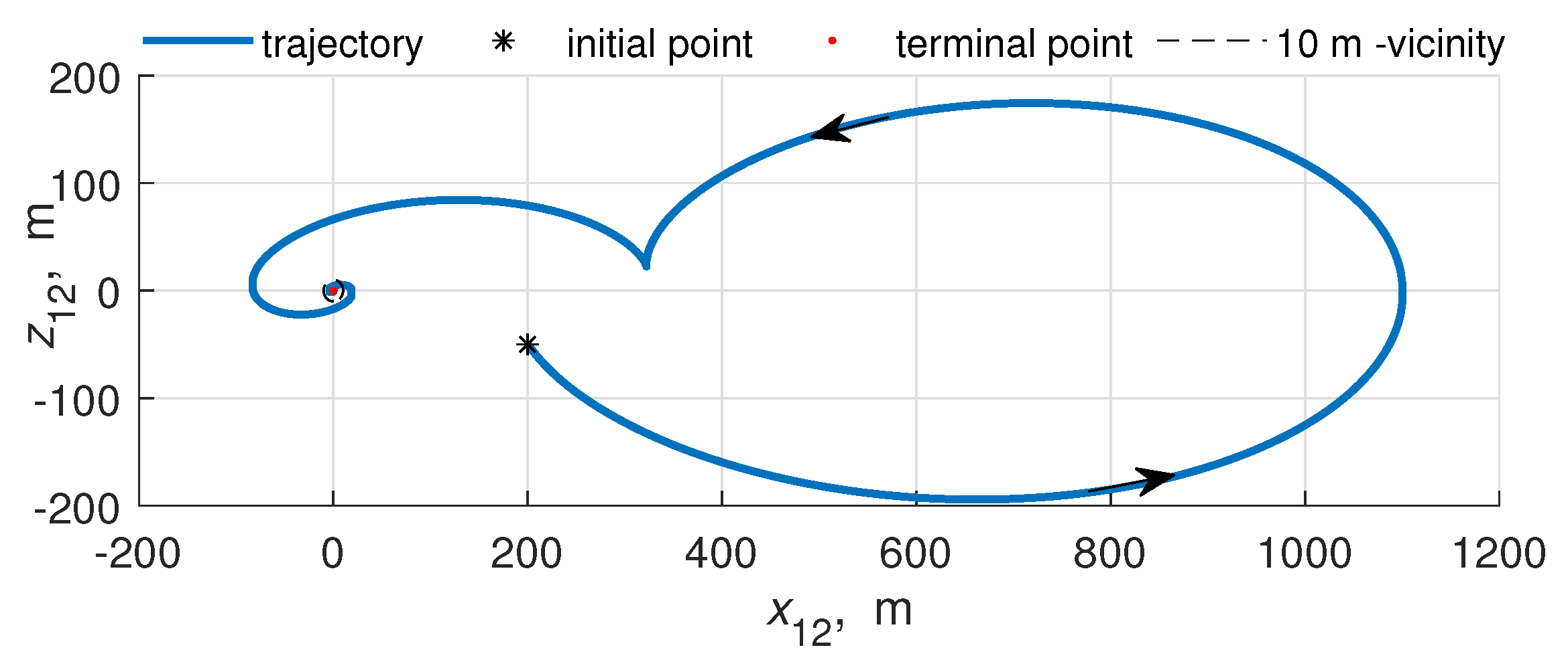
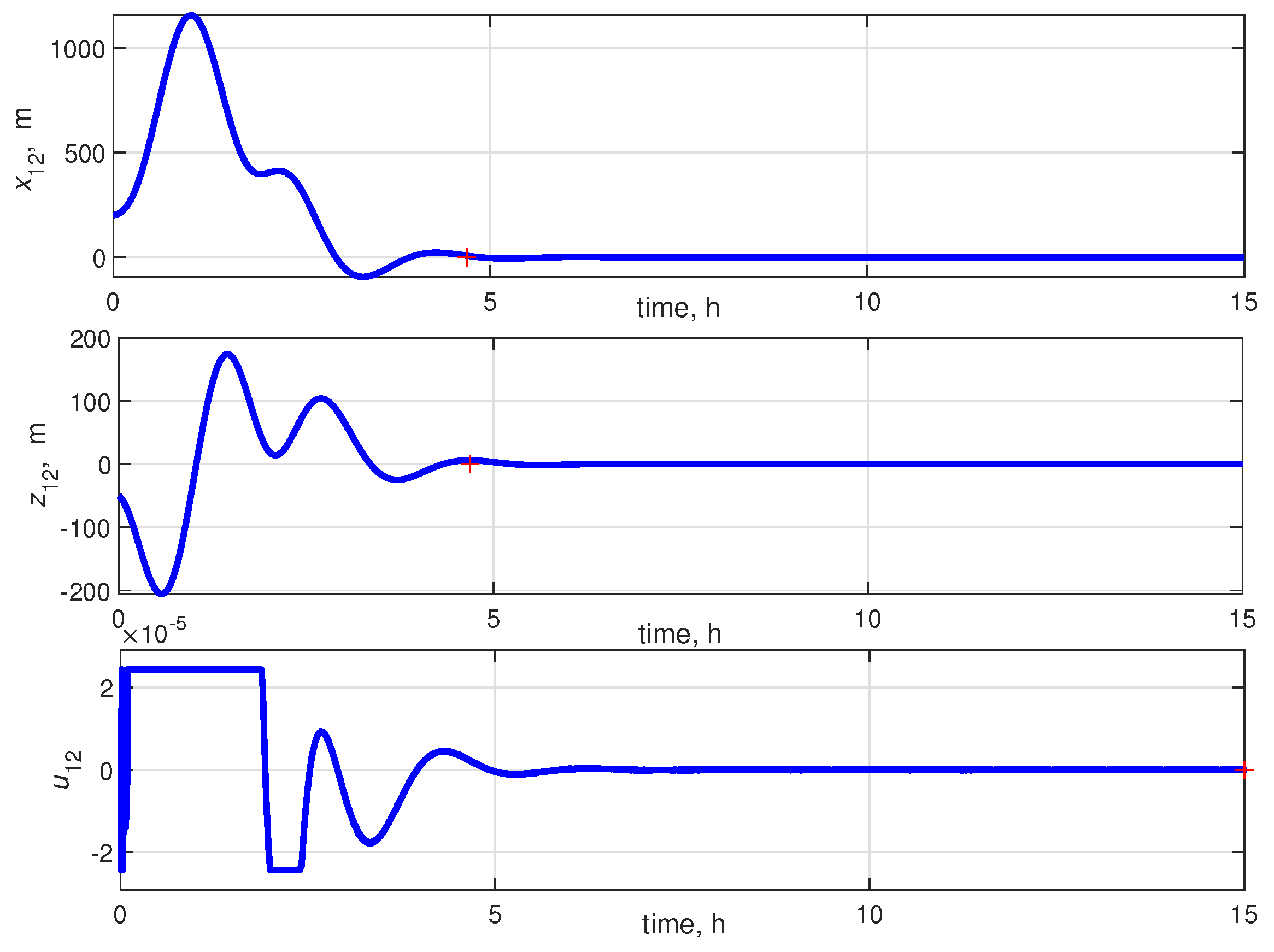
4.4.2. Simulations for Ideal Communication Channel

The simulations were performed in the MATLAB/Simulink software environment. For the numerical solution of the differential equations the MATLAB variable-step routine ode45 with the relative tolerance ${10}^{-3}$ was used. For hybrid (continuous–discrete systems), including the coding/decoding procedure model, the blocks from the standard Simulink/Discrete blockset were included. The simulation time was confined to $t_{\mathrm{fin}}=$ 54,000 s $=15$ h.

Firstly, consider the “ideal” case where the position information is transferred over the channel without sampling and level quantization. For the performance criterion, let as pick up instant $T^{*}$ when the relative trajectory on the $(X,Z)$ plane reaches the circle with given radius Q and does not leave it in the future, i.e., $T^{*}=\underset{t}{max}\left(\sqrt{x_{12}^2+z_{12}^2}>Q\right)$ ($T^{*}$ is further called the regulation time). It is natural to assume that within this circle the regulation rule switches to the rule ensuring collision avoidance, which is beyond the scope of this paper.

The simulation results for various initial conditions are depicted in Figure 2, Figure 3, Figure 4 and Figure 5. Figure 2 and Figure 3 are related to the case of $x_{12}\left(0\right)=20$ m, ${\dot{x}}_{12}\left(0\right)=0.05$ m/s, and other initial conditions are zero. Time histories of relative positions $x_{12}\left(t\right)$, $z_{12}\left(t\right)$ and control action $u\left(t\right)$ are plotted in Figure 2. Symbol “+” marks regulation time $T^{*}$. For the given initial conditions, $T^{*}=3.27$ h is obtained. Figure 4 and Figure 5 show similar plots for the case of $x_{12}\left(0\right)=200$ m, ${\dot{x}}_{12}\left(0\right)=0.025$ m/s, $z_{12}\left(0\right)=-50$ m, and ${\dot{z}}_{12}\left(0\right)=-0.025$ m/s. In this case, $T^{*}=4.61$ h.

The simulation results show that, despite of the control signal saturation at the beginning of the process, the targeting manifold is attained for both sets of the initial conditions with regulation time $T^{*}=3.27$ h (Figure 2 and Figure 3) and $T^{*}=4.61$ h (Figure 4 and Figure 5), respectively. Moreover, based on the harmonic balance method arguments [52,53] the conclusion can be made that the closed-loop system is globally asymptotically stable.

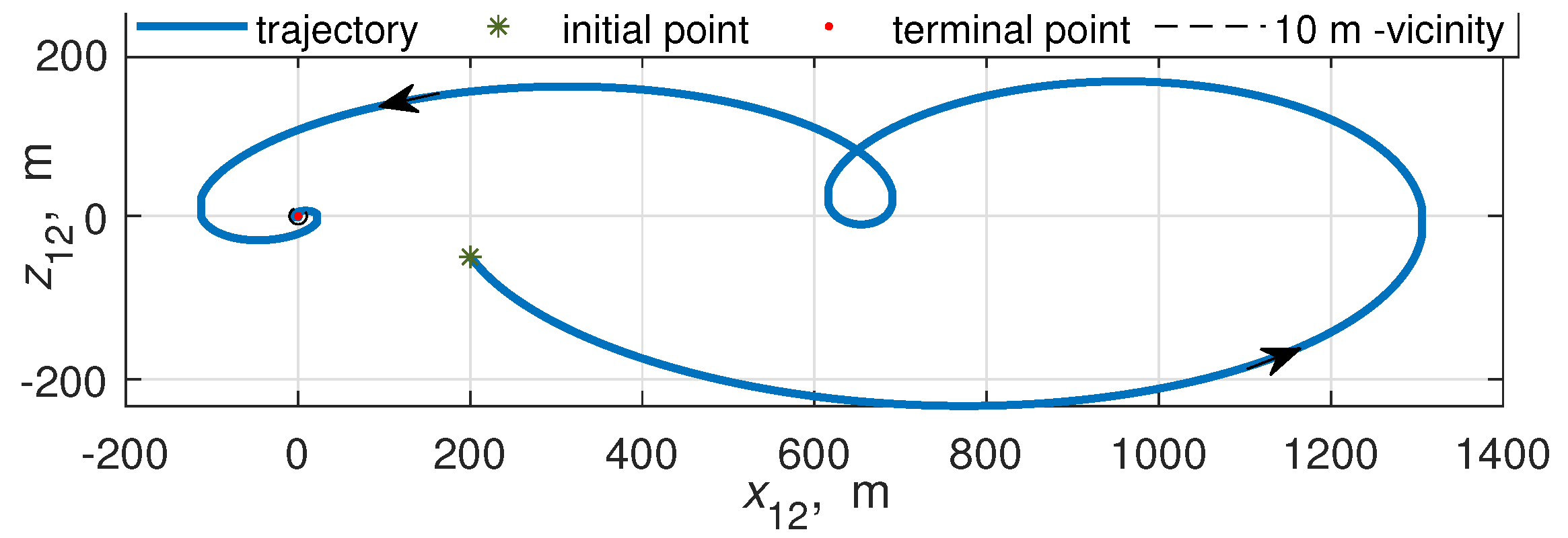
4.4.3. Satellite Position Transmission Over the Digital Communication Channel with Finite Capacity

Secondly, consider the case when the satellites exchange each other their LVLH coordinates over the binary communication channels, described in Section 2.2 and Section 4.2. It is assumed that each satellite transmits its coordinates $x_i$, $z_i$, $i=1,2$ to the accompanying one, where the estimates ${\widehat{x}}_i\left[k\right]$, ${\widehat{z}}_i\left[k\right]$ and ${\widehat{\dot{x}}}_i\left[k\right]$, ${\widehat{\dot{z}}}_i\left[k\right]$ are obtained. The following quantization and data transmission algorithms are used: Binary quantization (4), adaptive zooming (5), and embedded state estimation (17). For the numerical study, the coding-decoding procedure parameters are picked up as follows: $M_0=1$, $m_c=0$, $\rho =e^{-0.01T_0}$, gains $l_1$, $l_2$ of observer (17) are found by the pole-placement technique for the discrete-time system ${\widehat{y}}_{[}k+1]=\widehat{y}\left[k\right]+T_0\widehat{V}\left[k\right]+l_1{\sigma }_i\left[k\right]$, $\widehat{V}[k+1]=\widehat{V}\left[k\right]+l_2{\sigma }_i\left[k\right]$, where $y\left[k\right]$ and $V\left[k\right]$ are related to estimates ${\widehat{x}}_i\left[k\right]$, ${\widehat{z}}_i\left[k\right]$ and ${\widehat{\dot{x}}}_i\left[k\right]$, ${\widehat{\dot{z}}}_i\left[k\right]$ depending on the transmitted coordinate (x or z) and the satellite number $i=1,2$. Initial conditions $y\left[0\right]$, $V\left[0\right]$ are set to zero for all four channels. Therefore, two data transmission channels are supposed to be used on each satellite, so the data transmission rate for each binary communication channel $R=1/T_0$ should be doubled to find the overall channel load.

The simulation results for $T_0=0.667$ s ($R=1.5$ bit/s for each coordinate $x_i$ and $z_i$, transmitted from i-th satellite) and initial conditions $x_{12}\left(0\right)=200$ m, ${\dot{x}}_{12}\left(0\right)=0.025$ m/s, $z_{12}\left(0\right)=-50$ m, and ${\dot{z}}_{12}\left(0\right)=-0.025$ m/s are plotted in Figure 6 and Figure 7, where time histories of $x_{12}\left(t\right)$, $z_{12}\left(t\right)$, and $u\left(t\right)$ and the satellites relative trajectories on the (XZ) plane are depicted. Regulation time $T^{*}=4.84$ h is found by the simulation, which is a bit greater than the regulation time for non-restricted communication channel ($T^{*}=4.61$ h), compared with the plots on Figure 4 and Figure 5. The time histories and trajectories for the ideal and limited capacity communication channels differ due to the coder transient at the beginning of the coding procedure, which leads to oscillating control action during the certain transient time of the data transmission procedure. For avoiding these oscillations on practice, such measures as filtering of the control signal at the beginning of the process or the delayed start of the regulation, can be used.

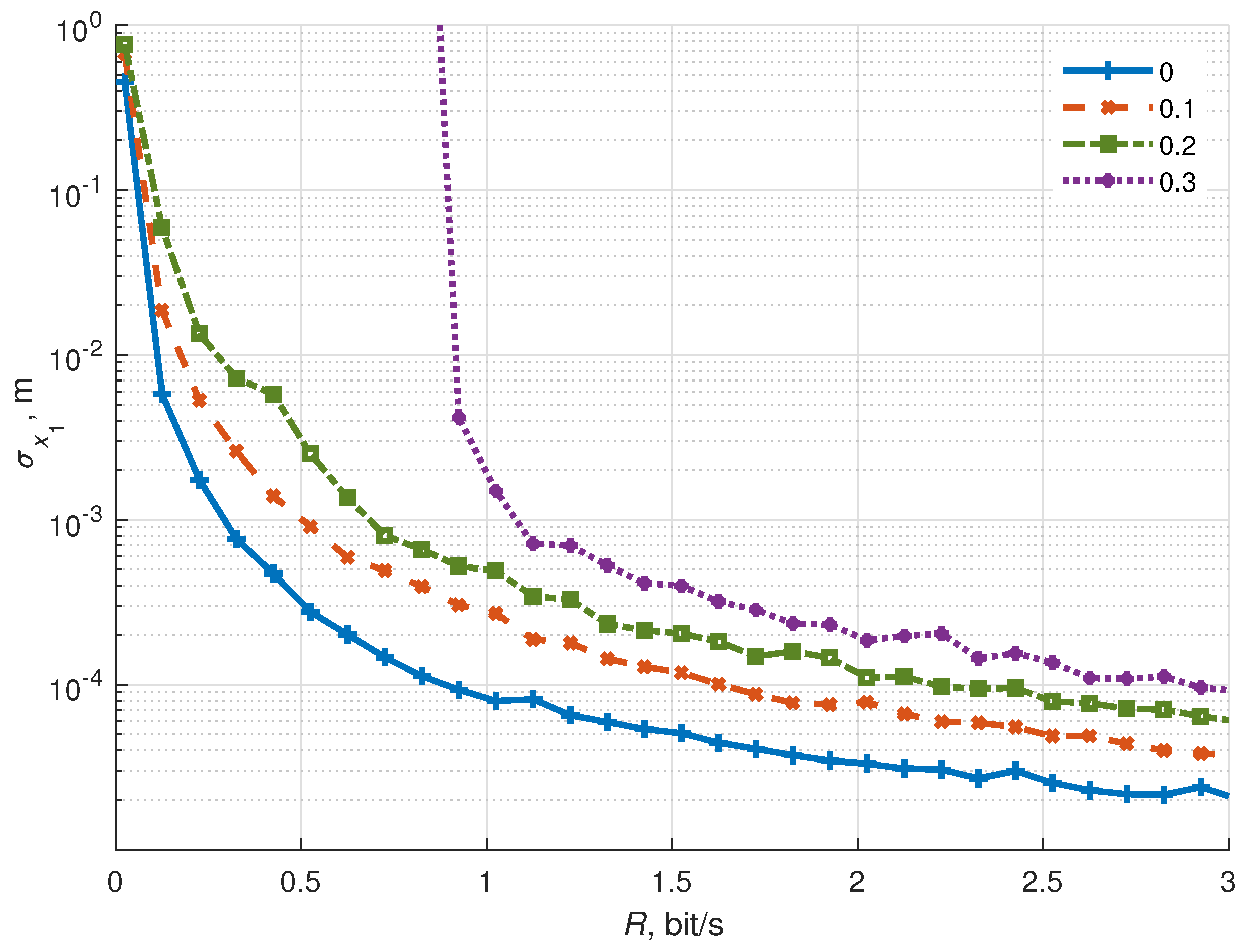
4.4.4. Case of Erasure Communication Channel

Thirdly, let us study how the erasure of data in the communication channel affects the data transmission accuracy and the regulation time for the relative position of the satellites.

For evaluating the data transmission accuracy, the transients of the transmission procedure were excluded by consideration only the last $0.3t_{\mathrm{fin}}$ interval of the simulation time. For this interval, the standard deviations ${\sigma }_{e_{x_1}}$ and ${\sigma }_{e_{{\dot{x}}_1}}$ of the data transmission errors $e_{x_1}\left[k\right]=x_1\left(t_k\right)-{\widehat{x}}_1\left(t_k\right)$, and $e_{{\dot{x}}_1}\left[k\right]={\dot{x}}_1\left(t_k\right)-{\widehat{\dot{x}}}_1\left(t_k\right)$ (respectively) were calculated. Logarithmically scaled functions ${\sigma }_{e_{x_1}}$, ${\sigma }_{e_{{\dot{x}}_1}}$ versus transmission rate R for various values of erasure probability p are plotted in Figure 8 and Figure 9. The plots show that the data transmission errors decrease monotonically, looking like inversely proportional functions on communication rate R and are practically negligibly small as $R>1$ bit/s for all considered values of p.

A summary graph of the dependence of regulation time $T^{*}$ on the data transmission rate R (for each one channel) at various erasure probabilities $p\in \{0,0.1,0.2,0.3\}$ is shown in Figure 10. The curves in Figure 10 make an impression about the required load of the communication channel and the quality of the stabilization process with its use. It is seen from the plot that for significantly high data transmission rate (exceeding 2 bit/s in our example) erasure of data in the channel with probability up to $0.3$ does not have an effect on the regulation time. This time is defined by the system dynamics regardless of the communication channel capacity.

To illustrate the system performance, the particular processes for $T_0=0.667$ s, $x_{12}\left(0\right)=200$ m, ${\dot{x}}_{12}\left(0\right)=0.025$ m/s, $z_{12}\left(0\right)=-50$ m, and ${\dot{z}}_{12}\left(0\right)=-0.025$ m/s and probability $p=0.2$ of erasing data in the communication channel are plotted in Figure 11 and Figure 12. Regulation time $T^{*}=7.07$ h is found by the simulation. The time histories and trajectories for the ideal and limited capacity erasure communication channels significantly differ from the case of the ideal channel, and from an application viewpoint, the process quality for these conditions is a boundary one.

Illustrations of the adaptive coding procedure are given in Figure 13 and Figure 14. Adaptively tuning quantizer range $M\left[k\right]$ in accordance with algorithm (5) is depicted in Figure 13. The plot shows how the range is automatically increased at the initial stage of the process and decays then, which leads to reducing the data transmission error. Figure 14 illustrates an influence of data erasure on the codewords, transmitted over the channel. Signal $s\left[k\right]$ from the coder is received in the form of $s_{\zeta }\left[k\right]$ on the decoder side. The difference between these signals causes the additional data transmission errors.

5. Conclusions

In the paper the feedback control law was designed ensuring the regulation of the relative satellites motion in a swarm. Unlike previous papers, the limited data transmission rate over the communication channels was taken into account. The adaptive coding/decoding procedure for the transmission of position between the satellites in the formation, employing the kinematics process description was studied for the cases of the ideal and erasure channel. Note that an adaptive coder used in the paper was not new since it was employed earlier for other problems in [77,78]. However such a coder was not applied to the control of satellite swarms previously and this is an additional novelty in the paper.

The dependence of the closed-loop system performance and accuracy of the data transmission algorithm on the data transmission rate was numerically evaluated. It was shown that both data transmission error and regulation time depend approximately inversely proportionally on the communication rate.

In future research, disturbances and noise in the communication channel will be taken into account.

References

1. Chang, I.; Chung, S.J.; Blackmore, L. Cooperative control with adaptive graph Laplacians for spacecraft formation flying. In Proceedings of the IEEE Conference Decision and Control (CDC 2010), Atlanta, GA, USA, 15–17 December 2010; pp. 4926–4933. [Google Scholar] [CrossRef] [Green Version]
2. Morgan, D.; Chung, S.J.; Blackmore, L.; Acikmese, B.; Bayard, D.; Hadaegh, F. Swarm-keeping strategies for spacecraft under J2 and atmospheric drag perturbations. J. Guid. Control Dyn. 2012, 35, 1492–1506. [Google Scholar] [CrossRef] [Green Version]
3. Monakhova, U.; Ivanov, D.; Roldugin, D. Magnetorquers attitude control for differential aerodynamic force application to nanosatellite formation flying construction and maintenance. Adv. Astronaut. Sci. 2020, 170, 385–397. [Google Scholar]
4. Kumar, B.; Ng, A.; Yoshihara, K.; De Ruiter, A. Differential drag as a means of spacecraft formation control. IEEE Trans. Aerosp. Electron. Syst. 2011, 47, 1125–1135. [Google Scholar] [CrossRef]
5. Pérez, D.; Bevilacqua, R. Lyapunov-based Spacecraft Rendezvous Maneuvers using Differential Drag. In Proceedings of the AIAA Guidance, Navigation, and Control Conference, Portland, OR, USA, 8–11 August 2011; pp. 2011–6630. [Google Scholar]
6. Varma, S.; Kumar, K. Multiple satellite formation flying using differential aerodynamic drag. J. Spacecr. Rocket. 2012, 49, 325–336. [Google Scholar] [CrossRef]
7. Horsley, M.; Nikolaev, S.; Pertica, A. Small satellite rendezvous using differential lift and drag. J. Guid. Control Dyn. 2013, 36, 445–453. [Google Scholar] [CrossRef]
8. Kumar, K.; Misra, A.; Varma, S.; Reid, T.; Bellefeuille, F. Maintenance of satellite formations using environmental forces. Acta Astronaut. 2014, 102, 341–354. [Google Scholar] [CrossRef]
9. Dellelce, L.; Kerschen, G. Optimal propellantless rendez-vous using differential drag. Acta Astronaut. 2015, 109, 112–123. [Google Scholar] [CrossRef]
10. Ivanov, D.; Monakhova, U.; Ovchinnikov, M. Nanosatellites swarm deployment using decentralized differential drag-based control with communicational constraints. Acta Astronaut. 2019, 159, 646–657. [Google Scholar] [CrossRef]
11. Ivanov, D.; Biktimirov, S.; Chernov, K.; Kharlan, A.; Monakhova, U.; Pritykin, D. Writing with Sunlight: Cubesat formation control using aerodynamic forces. In Proceedings of the 70th International Astronautical Congress, Washington, DC, USA, 21–25 October 2019. [Google Scholar]
12. Tang, A.; Wu, X. LEO satellite formation flying via differential atmospheric drag. Int. J. Space Sci. Eng. 2019, 5, 289–320. [Google Scholar] [CrossRef]
13. Shouman, M.; Bando, M.; Hokamoto, S. Output regulation control for satellite formation flying using differential drag. J. Guid. Control Dyn. 2019, 42, 2220–2232. [Google Scholar] [CrossRef]
14. Smith, B.; Capon, C.; Brown, M. Ionospheric drag for satellite formation control. J. Guid. Control Dyn. 2019, 42, 2590–2599. [Google Scholar] [CrossRef]
15. Traub, C.; Herdrich, G.; Fasoulas, S. Influence of energy accommodation on a robust spacecraft rendezvous maneuver using differential aerodynamic forces. CEAS Space J. 2020, 12, 43–63. [Google Scholar] [CrossRef]
16. Traub, C.; Romano, F.; Binder, T.; Boxberger, A.; Herdrich, G.; Fasoulas, S.; Roberts, P.; Smith, K.; Edmondson, S.; Haigh, S.; et al. On the exploitation of differential aerodynamic lift and drag as a means to control satellite formation flight. CEAS Space J. 2020, 12, 15–32. [Google Scholar] [CrossRef]
17. Leonard, C. Formationkeeping of Spacecraft via Differential Drag. Master’s Thesis, Massachusetts Institute of Technology, Cambridge, MA, USA, 1986. [Google Scholar]
18. Kim, D.Y.; Woo, B.; Park, S.Y.; Choi, K.H. Hybrid optimization for multiple-impulse reconfiguration trajectories of satellite formation flying. Adv. Space Res. 2009, 44, 1257–1269. [Google Scholar] [CrossRef]
19. Vaddi, S.; Alfriend, K.; Vadali, S.; Sengupta, P. Formation establishment and reconfiguration using impulsive control. J. Guid. Control Dyn. 2005, 28, 262–268. [Google Scholar] [CrossRef]
20. Vaddi, S. Modeling and Control of Satellite Formations. Ph.D. Thesis, Department of Aerospace Engineering, Texas A&M University, College Station, TX, USA, 2003. [Google Scholar]
21. Monakhova, U.; Ivanov, D. Formation of a Swarm of Nanosatellites Using Decentralized Aerodynamic Control, Taking into Account Communication Constraints; M.V. Keldysh Institute Preprints; Keldysh Institute: Moscow, Russia, 2018; (In Russian). [Google Scholar] [CrossRef]
22. Sarno, S.; D’Errico, M.; Guo, J.; Gill, E. Path planning and guidance algorithms for SAR formation reconfiguration: Comparison between centralized and decentralized approaches. Acta Astronaut. 2020, 167, 404–417. [Google Scholar] [CrossRef]
23. Basu, S.; Groves, K.; Basu, S.; Sultan, P. Specification and forecasting of scintillations in communication/navigation links: Current status and future plans. J. Atmos. Sol. Terr. Phys. 2002, 64, 1745–1754. [Google Scholar] [CrossRef]
24. Freimann, A.; Petermann, T.; Schilling, K. Interference-Free Contact Plan Design for Wireless Communication in Space-Terrestrial Networks. In Proceedings of the 2019 IEEE International Conference on Space Mission Challenges for Information Technology (SMC-IT), Pasadena, CA, USA, 30 July–1 August 2019; pp. 55–61. [Google Scholar] [CrossRef]
25. Zhao, Y.; Yi, X.; Hou, Z.; Zhang, Y.; Li, C. Parallel data transmission for navigation satellite network with agility link. Int. J. Satell. Commun. Netw. 2019, 37, 536–550. [Google Scholar] [CrossRef]
26. Cai, X.; Zhou, M.; Xia, T.; Fong, W.; Lee, W.T.; Huang, X. Low-Power SDR Design on an FPGA for Intersatellite Communications. IEEE Trans. Large Scale Integr. Syst. 2018, 26, 2419–2430. [Google Scholar] [CrossRef]
27. Davarian, F.; Asmar, S.; Angert, M.; Baker, J.; Gao, J.; Hodges, R.; Israel, D.; Landau, D.; Lay, N.; Torgerson, L.; et al. Improving Small Satellite Communications and Tracking in Deep Space—A Review of the Existing Systems and Technologies with Recommendations for Improvement. Part II: Small Satellite Navigation, Proximity Links, and Communications Link Science. IEEE Aerosp. Electron. Syst. Mag. 2020, 35, 26–40. [Google Scholar] [CrossRef]
28. Poomagal, C.; Sathish Kumar, G. ECC Based Lightweight Secure Message Conveyance Protocol for Satellite Communication in Internet of Vehicles (IoV). Wirel. Pers. Commun. 2020, 113, 1359–1377. [Google Scholar] [CrossRef]
29. Ujan, S.; Navidi, N.; Landry, R.J. Hierarchical classification method for radio frequency interference recognition and characterization in satcom. Appl. Sci. 2020, 10, 4608. [Google Scholar] [CrossRef]
30. Kuang, Y.; Yi, X.; Hou, Z. Congestion avoidance routing algorithm for topology-inhomogeneous low earth orbit satellite navigation augmentation network. Int. J. Satell. Commun. Netw. 2020. [Google Scholar] [CrossRef]
31. Nair, G.; Evans, R. Exponential stabilisability of finite-dimensional linear systems with limited data rates. Automatica 2003, 39, 585–593. [Google Scholar] [CrossRef]
32. Bazzi, L.; Mitter, S. Endcoding complexity versus minimum distance. IEEE Trans. Inform. Theory 2005, 51, 2103–2112. [Google Scholar] [CrossRef]
33. Nair, G.; Fagnani, F.; Zampieri, S.; Evans, R. Feedback control under data rate constraints: An overview. Proc. IEEE 2007, 95, 108–137. [Google Scholar] [CrossRef]
34. Matveev, A.; Savkin, A. Estimation and Control over Communication Networks; Birkhäuser: Boston, MA, USA, 2009. [Google Scholar]
35. Andrievsky, B.; Matveev, A.; Fradkov, A. Control and estimation under information constraints: Toward a unified theory of control, computation and communications. Autom. Remote Control 2010, 71, 572–633. [Google Scholar] [CrossRef]
36. Kwakernaak, H.; Sivan, R. Linear Optimal Control Systems; Wiley-Interscience: New York, NY, USA, 1972. [Google Scholar]
37. Nair, G.; Evans, R. Stabilizability of stochastic linear systems with finite feedback data rates. SIAM J. Control Optim. 2004, 43, 413–436. [Google Scholar] [CrossRef] [Green Version]
38. Nair, G.; Evans, R.; Mareels, I.; Moran, W. Topological feedback entropy and nonlinear stabilization. IEEE Trans. Automat. Control 2004, 49, 1585–1597. [Google Scholar] [CrossRef]
39. Fradkov, A.; Andrievsky, B.; Evans, R. Chaotic observer-based synchronization under information constraints. Phys. Rev. E 2006, 73, 066209. [Google Scholar] [CrossRef] [Green Version]
40. Cover, T.; Thomas, J. Elements of Information Theory; John Wiley & Sons, Inc.: New York, NY, USA; Chichester, UK; Brisbane, Australia; Toronto, ON, Canada; Singapore, 1991. [Google Scholar]
41. Rizzo, L. Effective Erasure Codes for Reliable Computer Communication Protocols. Comput. Commun. Rev. 1997, 27, 24–36. [Google Scholar] [CrossRef] [Green Version]
42. Tatikonda, S.; Mitter, S. Control Over Noisy Channels. IEEE Trans. Automat. Control 2004, 49, 1196–1201. [Google Scholar] [CrossRef]
43. Shokrollahi, A. Raptor codes. IEEE Trans. Inform. Theory 2006, 52, 2551–2567. [Google Scholar] [CrossRef]
44. Köetter, R.; Kschischang, F. Coding for Errors and Erasures in Random Network Coding. IEEE Trans. Inform. Theory 2008, 54, 3579–3591. [Google Scholar] [CrossRef]
45. Patterson, S.; Bamieh, B.; El Abbadi, A. Convergence Rates of Distributed Average Consensus With Stochastic Link Failures. IEEE Trans. Automat. Control 2010, 55, 880–892. [Google Scholar] [CrossRef]
46. Diwadkar, A.; Vaidya, U. Robust synchronization in nonlinear network with link failure uncertainty. In Proceedings of the 50th IEEE Conference Decision and Control and European Control Conference (CDC-ECC 2011), Orlando, FL, USA, 12–15 December 2011; IEEE: Orlando, FL, USA, 2011; pp. 6325–6330. [Google Scholar]
47. Wang, J.; Yan, Z. Coding scheme based on spherical polar coordinate for control over packet erasure channel. Int. J. Robust Nonlinear Control 2014, 24, 1159–1176. [Google Scholar] [CrossRef]
48. Zhang, H.; Lee, S.; Li, X.; He, J. EEG self-adjusting data analysis based on optimized sampling for robot control. Electronics 2020, 9, 925. [Google Scholar] [CrossRef]
49. Jeon, S.; Park, C.; Seo, D. The multi-station based variable speed limit model for realization on urban highway. Electronics 2020, 9, 801. [Google Scholar] [CrossRef]
50. Tsypkin, Y. Stability and sensitivity of nonlinear sampled data systems. In Sensitivity Methods in Control Theory; Radanovic, L., Ed.; Pergamon: Oxford, UK, 1966; pp. 46–66. [Google Scholar] [CrossRef]
51. Pogromsky, A.; Matveev, A. A non-quadratic criterion for stability of forced oscillation. Syst. Control Lett. 2013, 62, 408–412. [Google Scholar] [CrossRef]
52. Dudkowski, D.; Jafari, S.; Kapitaniak, T.; Kuznetsov, N.V.; Leonov, G.A.; Prasad, A. Hidden attractors in dynamical systems. Phys. Rep. 2016, 637, 1–50. [Google Scholar] [CrossRef]
53. Kuznetsov, N. Theory of hidden oscillations and stability of control systems. J. Comput. Syst. Sci. Int. 2020, 59, 647–668. [Google Scholar] [CrossRef]
54. Hespanha, J.P.; Naghshtabrizi, P.; Xu, Y. A Survey of Recent Results in Networked Control Systems. Proc. IEEE 2007, 95, 138–162. [Google Scholar] [CrossRef] [Green Version]
55. Xia, Y.Q.; Gao, Y.L.; Yan, L.P.; Fu, M.Y. Recent progress in networked control systems—A survey. Intern. J. Autom. Comput. 2015, 12, 343–367. [Google Scholar] [CrossRef]
56. Nair, G.; Evans, R. State estimation via a capacity-limited communication channel. In Proceedings of the 36th IEEE Conference on Decision and Control (CDC’97), San Diego, CA, USA, 10–12 December 1997; pp. 866–871. [Google Scholar]
57. Andrievsky, B.; Fradkov, A.L. Control and observation via communication channels with limited bandwidth. Gyroscopy Navig. 2010, 1, 126–133. [Google Scholar] [CrossRef]
58. De Persis, C. n-Bit stabilization of n-dimensional nonlinear systems in feedforward form. IEEE Trans. Automat. Control 2005, 50, 299–311. [Google Scholar] [CrossRef]
59. Liberzon, D.; Hespanha, J. Stabilization of nonlinear systems with limited information feedback. IEEE Trans. Automat. Control 2005, 50, 910–915. [Google Scholar] [CrossRef] [Green Version]
60. Matveev, A.; Proskurnikov, A.; Pogromsky, A.; Fridman, E. Comprehending complexity: Data-rate constraints in large-scale networks. IEEE Trans. Automat. Control 2019, 64, 4252–4259. [Google Scholar] [CrossRef]
61. Voortman, Q.; Pogromsky, A.; Matveev, A.; Nijmeijer, H. Data-rate constrained observers of nonlinear systems. Entropy 2019, 21, 282. [Google Scholar] [CrossRef] [Green Version]
62. Matveev, A.; Pogromsky, A. Observation of nonlinear systems via finite capacity channels, Part II: Restoration entropy and its estimates. Automatica 2019, 103, 189–199. [Google Scholar] [CrossRef]
63. Åström, K.J.; Bernhardsson, B.M. Comparison of Riemann and Lebesgue sampling for first order stochastic systems. In Proceedings of the 41st IEEE Conference on Decision & Control (CDC 2002), Las Vegas, NV, USA, 10–13 December 2002; pp. 2011–2016. [Google Scholar]
64. Yu, H.; Antsaklis, P.J. Output Synchronization of Networked Passive Systems With Event-Driven Communication. IEEE Trans. Automat. Control 2014, 59, 750–756. [Google Scholar] [CrossRef]
65. Margun, A.; Furtat, I.; Zimenko, K.; Kremlev, A. Event-triggered output robust controller. In Proceedings of the 25th Mediterranean Conf. Control Automation (MED 2017), Valletta, Malta, 3–6 July 2017; pp. 625–630. [Google Scholar] [CrossRef]
66. Li, K.; Baillieu, J. Robust quantization for digital finite communication bandwidth (DFCB) control. IEEE Trans. Automat. Control 2004, 49, 1573–1584. [Google Scholar] [CrossRef]
67. Gabor, G.; Gyorfi, Z. Recursive Source Coding; Springer: New York, NY, USA, 1986. [Google Scholar]
68. Tatikonda, S.; Sahai, A.; Mitter, S. Control of LQG Systems Under Communication Constraints. In Proceedings of the 37th IEEE Conference Decision and Control, Tampa, FL, USA, 18 December 1998; IEEE: Tampa, FL, USA, 1998; Volume WP04, pp. 1165–1170. [Google Scholar]
69. Brockett, R.; Liberzon, D. Quantized feedback stabilization of linear systems. IEEE Trans. Automat. Control 2000, 45, 1279–1289. [Google Scholar] [CrossRef] [Green Version]
70. Liberzon, D. Hybrid feedback stabilization of systems with quantized signals. Automatica 2003, 39, 1543–1554. [Google Scholar] [CrossRef]
71. Tatikonda, S.; Mitter, S. Control under communication constraints. IEEE Trans. Automat. Control 2004, 49, 1056–1068. [Google Scholar] [CrossRef] [Green Version]
72. Fradkov, A.; Andrievsky, B.; Ananyevskiy, M. State estimation and synchronization of pendula systems over digital communication channels. Eur. Phys. J. Spec. Top. 2014, 223, 773–793. [Google Scholar] [CrossRef]
73. Fradkov, A.L.; Andrievsky, B.; Evans, R.J. Adaptive Observer-Based Synchronization of Chaotic Systems with First-Order Coder in Presence of Information Constraints. IEEE Trans. Circuits Syst. I 2008, 55, 1685–1694. [Google Scholar] [CrossRef]
74. Fradkov, A.; Andrievsky, B.; Evans, R. Synchronization of passifiable Lurie systems via limited-capacity communication channel. IEEE Trans. Circuits Syst. I 2009, 56, 430–439. [Google Scholar] [CrossRef]
75. Moreno-Alvarado, R.; Rivera-Jaramillo, E.; Nakano, M.; Perez-Meana, H. Simultaneous Audio Encryption and Compression Using Compressive Sensing Techniques. Electronics 2020, 9, 863. [Google Scholar] [CrossRef]
76. Goodman, D.; Gersho, A. Theory of an adaptive quantizer. IEEE Trans. Commun. 1974, COM-22, 1037–1045. [Google Scholar] [CrossRef]
77. Andrievsky, B.; Fradkov, A. Adaptive coding for position estimation in formation flight control. IFAC Proc. Vol. 2010, 1, 72–76. [Google Scholar] [CrossRef]
78. Fradkov, A.; Andrievsky, B.; Peaucelle, D. Estimation and control under information constraints for LAAS helicopter benchmark. IEEE Trans. Control Syst. Technol. 2010, 18, 1180–1187. [Google Scholar] [CrossRef]
79. Gomez-Estern, F.; Canudas de Wit, C.; Rubio, F. Adaptive delta modulation in networked controlled systems with bounded disturbances. IEEE Trans. Automat. Control 2011, 56, 129–134. [Google Scholar] [CrossRef]
80. Hill, G.W. Researches in the Lunar Theory. Am. J. Math. 1878, 1, 5–26. [Google Scholar] [CrossRef]
81. Clohessy, W.; Wiltshire, R. Terminal guidance system for satellite rendezvous. J. Aerosp. Sci. 1960, 653–658. [Google Scholar] [CrossRef]
82. Sedwick, R.; Miller, D.; Kong, E. Mitigation of Differential Perturbations. J. Astronaut. Sci. 1999, 47, 309–331. [Google Scholar] [CrossRef]
83. Schweighart, S.; Sedwick, R. High-Fidelity Linearized J2 Model for Satellite Formation Flight. J. Guid. Control Dyn. 2002, 25, 1073–1080. [Google Scholar] [CrossRef]
84. Schlanbusch, R.; Kristiansen, R.; Nicklasson, P. Spacecraft formation reconfiguration with collision avoidance. Automatica 2011, 47, 1443–1449. [Google Scholar] [CrossRef]
85. Renga, A.; Grassi, M.; Tancredi, U. Relative navigation in LEO by carrier-phase differential GPS with intersatellite ranging augmentation. Int. J. Aerosp. Eng. 2013, 2013, 627509. [Google Scholar] [CrossRef] [Green Version]
86. Fradkov, A.L.; Miroshnik, I.V.; Nikiforov, V.O. Nonlinear and Adaptive Control of Complex Systems; Kluwer: Dordrecht, The Netherlands, 1999. [Google Scholar]
87. Andrievsky, B.; Kudryashova, E.; Kuznetsov, N.; Kuznetsova, O. Aircraft wing rock oscillations suppression by simple adaptive control. Aerosp. Sci. Technol. 2020, 105, 1–10. [Google Scholar] [CrossRef]
88. Massey, T.; Shtessel, Y. Continuous Traditional and High-Order Sliding Modes for Satellite Formation Control. J. Guid. Control Dyn. 2005, 28, 826–831. [Google Scholar] [CrossRef]
89. Wu, S.; Sun, X.; Sun, Z.; Wu, X. Sliding-mode control for staring-mode spacecraft using a disturbance observer. Inst. Mech. Eng. Part G J. Aerosp. Eng. 2010, 224, 215–224. [Google Scholar] [CrossRef]
90. Cong, B.L.; Liu, X.D.; Chen, Z. Distributed attitude synchronization of formation flying via consensus-based virtual structure. Acta Astronaut. 2011, 68, 1973–1986. [Google Scholar] [CrossRef]
91. La Scala, B.; Evans, R. Minimum necessary data rates for accurate track fusion. In Proceedings of the 44th IEEE Conference on Decision and Control, and the European Control Conference, Seville, Spain, 12–15 December 2005; IEEE: Seville, Spain, 2005; pp. 6966–6971. [Google Scholar]
92. Evans, R.; Krishnamurthy, V.; Nair, G.; Sciacca, L. Networked sensor management and data rate control for tracking maneuvering targets. IEEE Trans. Signal Process. 2005, 53, 1979–1991. [Google Scholar] [CrossRef]
93. Tomashevich, S.; Andrievsky, B.; Fradkov, A.L. Formation control of a group of unmanned aerial vehicles with data exchange over a packet erasure channel. In Proceedings of the 1st IEEE Intern. Conf. Industrial Cyber-Physical Systems (ICPS 2018), Saint Petersburg, Russia, 15–18 May 2018; pp. 38–43. [Google Scholar] [CrossRef]
94. Andrievsky, B. Numerical evaluation of controlled synchronization for chaotic Chua systems over the limited-band data erasure channel. Cybern. Phys. 2016, 5, 3–51. [Google Scholar]
Figure 1. Coordinate system associated with reference point O, moving in a circular orbit.
Electronics 09 02032 g001
Figure 2. Time histories of x 12 ( t ) (upper plot), z 12 ( t ) (middle plot), and u ( t ) (lower). The ideal channel case. x 12 ( 0 ) = 20 m, x ˙ 12 ( 0 ) = 0.05 m/s; T * = 3.27 h.
Electronics 09 02032 g002
Figure 3. Satellites relative trajectories on the (XZ) plane for x 12 ( 0 ) = 20 m, x ˙ 12 ( 0 ) = 0.05 m/s. The ideal channel case. T * = 3.27 h.
Electronics 09 02032 g003
Figure 4. Time histories of x 12 ( t ) (upper plot), z 12 ( t ) (middle plot), and u ( t ) (lower plot). The ideal channel case. x 12 ( 0 ) = 200 m, x ˙ 12 ( 0 ) = 0.025 m/s, z 12 ( 0 ) = 50 m, z ˙ 12 ( 0 ) = 0.025 m/s; T * = 4.61 h.
Electronics 09 02032 g004
Figure 5. Satellites relative trajectories on the (XZ) plane for x 12 ( 0 ) = 200 m, x ˙ 12 ( 0 ) = 0.025 m/s, z 12 ( 0 ) = 50 m, z ˙ 12 ( 0 ) = 0.025 m/s. The ideal channel case. T * = 4.61 h.
Electronics 09 02032 g005
Figure 6. Time histories of x 12 ( t ) (upper plot), z 12 ( t ) (middle plot), and u ( t ) (lower plot). Case of quantization, R = 1.5 bit/s, p = 0 . x 12 ( 0 ) = 200 m, x ˙ 12 ( 0 ) = 0.025 m/s, z 12 ( 0 ) = 50 m, z ˙ 12 ( 0 ) = 0.025 m/s; T * = 4.69 h.
Electronics 09 02032 g006
Figure 7. Satellites relative trajectories on the (XZ) plane for x 12 ( 0 ) = 200 m, x ˙ 12 ( 0 ) = 0.025 m/s, z 12 ( 0 ) = 50 m, z ˙ 12 ( 0 ) = 0.025 m/s. Case of quantization, R = 1.5 bit/s, p = 0 . T * = 4.69 h.
Electronics 09 02032 g007
Figure 8. Data transmission error σ x 1 vs transmission rate R for various erasure probability p values.
Electronics 09 02032 g008
Figure 9. Data transmission error σ x ˙ 1 vs transmission rate R for various erasure probability p values.
Electronics 09 02032 g009
Figure 10. Regulation time T * vs transmission rate R for various erasure probability p values.
Electronics 09 02032 g010
Figure 11. Time histories of x 12 ( t ) (upper plot), z 12 ( t ) (middle plot), and u ( t ) (lower plot). Case of quantization and erasure, R = 1.5 bit/s, p = 0.2 . x 12 ( 0 ) = 200 m, x ˙ 12 ( 0 ) = 0.025 m/s, z 12 ( 0 ) = 50 m, z ˙ 12 ( 0 ) = 0.025 m/s; T * = 7.07 h.
Electronics 09 02032 g011
Figure 12. Satellites relative trajectories on the (XZ) plane for x 12 ( 0 ) = 200 m, x ˙ 12 ( 0 ) = 0.025 m/s, z 12 ( 0 ) = 50 m, z ˙ 12 ( 0 ) = 0.025 m/s. Case of quantization and erasure, R = 1.5 bit/s, p = 0.2 . T * = 7.07 h.
Electronics 09 02032 g012
Figure 13. Quantizer range M [ k ] time history for the case of quantization and erasure, R = 1.5 bit/s, p = 0.2 . x 12 ( 0 ) = 200 m, x ˙ 12 ( 0 ) = 0.025 m/s, z 12 ( 0 ) = 50 m, z ˙ 12 ( 0 ) = 0.025 m/s; T * = 7.07 h.
Electronics 09 02032 g013
Figure 14. Time histories of s [ k ] on the coder side (marked by the red circles) and s ζ [ k ] (marked by the blue dots) on the decoder side. Case of quantization and erasure, R = 1.5 bit/s, p = 0.2 . x 12 ( 0 ) = 200 m, x ˙ 12 ( 0 ) = 0.025 m/s, z 12 ( 0 ) = 50 m, z ˙ 12 ( 0 ) = 0.025 m/s; T * = 7.07 h.
Electronics 09 02032 g014
Publisher’s Note: MDPI stays neutral with regard to jurisdictional claims in published maps and institutional affiliations.