Correlation in MIMO Antennas

Abstract

Multiple-input multiple-output (MIMO) antennas are commonly evaluated by using the correlation coefficient. However, the correlation has several different definitions and calculation methods, and this misleads the real performance of the MIMO antennas. This paper describes five definitions and their differences of the correlation, i.e., signal correlation, channel correlation, fading correlation, complex pattern correlation, and S-parameter-based correlation. The difference of these characteristics is theoretically and numerically discussed, and their relations are schematically presented. Furthermore, the relationship between the correlation coefficient and the antenna element spacing is numerically evaluated, and it is shown that correlation coefficient calculated only from the S-parameter yields the error greater than 10% when the efficiency of the antenna is lower than 97%.

1. Introduction

A multiple-input multiple-output (MIMO) system achieves high-frequency utilization efficiency by simultaneously transmitting different signals using multiple antennas at both transmission and reception sides [1,2]. MIMO technology is being actively implemented to overcome the shortage of frequency resources caused by the dramatic advent of various kinds of wireless systems.

The performance of MIMO systems is determined by both radio propagation and antenna characteristics. The radio wave propagation characteristics are decided by the spatial relationships of the antennas and the surrounding environment such as buildings, making it difficult to realize the desired characteristics. Fortunately, the multiplicity of antennas offers significant design freedom and thus the possibility of improving MIMO channel capacity if the antenna design suits the given environment well.

To design a MIMO antenna that has high channel capacity, it is required to realize high efficiency and low correlation characteristics. While the consideration of efficiency in antenna design is quite general and well understood, the consideration of correlation characteristics is not simple. This is because calculating the correlation requires either channel models [3,4,5,6,7] or full two-dimensional (2D) complex patterns (note that ‘three-dimensional’ is incorrect because the pattern is normally defined by two variables, e.g., $\theta$ and $\varphi$).

As described above, the correlation is not as simple to calculate as other antenna characteristics. Hence, the S-parameter-based correlation coefficients proposed by Blanch [8] have been used in many studies [9]. Strictly speaking, a similar method was reported before Blanch’s paper, but the different term, ‘beam coupling factor’ was used instead of the correlation coefficient [10], and the demand for such antenna evaluation at that time was less than it is at present. The correlation coefficient is easy to evaluate through the use of the S-parameter if a multi-port network analyzer is available. However, this approach is not applicable to antennas with Joule heat loss because the radiation efficiency of the antenna excluding reflection loss and mutual coupling loss must be close to 100%. Hence, this equation should be carefully used by considering the principle and applicable conditions.

As for S-parameter-based correlation coefficients in lossy MIMO antenna, the uncertainty of the correlation coefficients is discussed in [11], where the radiation efficiency of the antennas is taken into account. It is mentioned that the uncertainty of the correlation coefficient is $\pm 1$ when the antenna efficiency of two antenna array is 50%, and this means the S-parameter-based correlation coefficient does not provide any information about the performance of MIMO antenna. A very interesting example is demonstrated in [12], where a single monopole antenna is connected to a Wilkinson divider that extends a single antenna port to two ports. This yields zero-correlation characteristics in the equation [8] since the divider completely isolates two extended ports. However, two extended ports always observe completely the same signals, i.e., the observed signals at two ports are fully correlated. To resolve the problem of the S-parameter based correlation in lossy MIMO antenna, the correction methods have been presented [12,13]. The work [14] compares the performance of these correction techniques numerically and experimentally, and the accuracy of the correction methods is discussed. It is concluded that the equivalent-circuit-based technique [13] yields better accuracy, but this requires measuring the radiation efficiency and selecting the adequate circuit model by considering the structure of the MIMO antenna. This alludes to the important relationship among the antenna geometry and characteristics.

Figure 1 conceptualizes the impact of three key antenna factors (impedance, pattern, size) on the correlation characteristics. The impedance characteristics can be conditionally translated into the correlation characteristics [8]. In addition, the complex pattern is directly translated into the correlation characteristics [10], and it is well known that low correlation coefficients can be attained if the patterns or polarizations are orthogonal [15,16,17,18,19]. It is also empirically known that correlation increases when the array antenna is small [20].

This paper deals with five correlation coefficients: signal correlation, channel correlation, fading correlation, complex pattern correlation, and S-parameter-based correlation. The main contributions of this paper are listed as follows:

(a)

Categorizing the correlation coefficients used in MIMO antenna evaluation.

(b)

Clarifying the commutativity among the correlation characteristics and some of the physical quantities

The remainder of this paper is organized as follows. Section 2 describes the signal model dealt with in this paper and the five definitions of the correlation coefficient in MIMO antenna, and their categories and relations are mentioned in detail. Section 3 presents the simulation results and discusses the problem in the S-parameter-based correlation by comparing correlation coefficient errors. Finally, the conclusion is drawn in Section 4.

2. Definitions and Computations of Correlation Coefficients

2.1. MIMO Signal Model

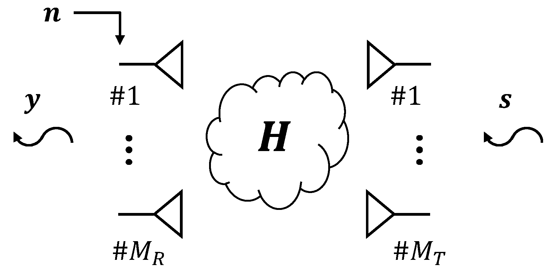
First, the MIMO signal model is defined in this section for the following discussions. Figure 2 shows the MIMO signal model considered in this paper; $M_T$ and $M_R$ are the numbers of transmitting and receiving antennas, respectively. $\mathit{H}$ is the channel matrix, which is defined as,

$$\begin{array}{c}\hfill \mathit{H}=\left(\begin{array}{ccc}{h}_{11}& \cdots & h_{1M_T}\\ ⋮& \ddots & ⋮\\ h_{M_{R}1}& \cdots & h_{M_R{M}_T}\end{array}\right),\end{array}$$

(1)

where $h_{kl}$ is the complex transfer function linking the l-th transmitting antenna to the k-th receiving antenna. The signal model for such a MIMO system is expressed as

$$\begin{array}{c}\hfill \mathit{y}=\mathit{H}\mathit{s}+\mathit{n},\end{array}$$

(2)

where $\mathit{s}$ is a column vector expressed as $\mathit{s}={(s_1,\cdots ,s_{M_T})}^T$ (${\{·\}}^T$ represents transposition of vector or matrix). Each of its entries represents the signal transmitted by each antenna element. $\mathit{y}$ is the received signal vector expressed as $\mathit{y}={(y_1,\cdots ,y_{M_R})}^T$, and $\mathit{n}$ is the noise vector expressed as $\mathit{n}={(n_1,\cdots ,n_{M_R})}^T$. All of the elements of $\mathit{s}$ and $\mathit{n}$ are independently distributed Gaussian random variables with zero mean. Note that ‘uncorrelated’ does not mean ‘independent’.

2.2. Received Signal Correlation

The correlation coefficient is used to evaluate the relationship between two series of signals. When we have two zero-mean complex signal series, $x_1$ and $x_2$, the complex correlation coefficient is defined as

$$\begin{array}{c}\hfill \rho =\frac{E\left[x_1{x}_2^{*}\right]}{\sqrt{E\left[\right|x_1{|}^2\left]E\right[|x_2{|}^2]}},\end{array}$$

(3)

where ${\{·\}}^{*}$ denotes complex conjugate, and $E[·]$ represents ensemble average. Equation (3) can be used to compute the correlation between the complex signals observed at two antennas. Note that $\rho$ is a complex value, and the range of the correlation value is $0\le \left|\rho \right|\le 1$.

Next, the definition of the signal correlation matrix is discussed. When the signal changes with time t, the correlation matrix of the received signal is written as

$$\begin{array}{ccc}\hfill {\mathit{R}}_{yy}& =& E\left[\mathit{y}\left(t\right){\mathit{y}}^H\left(t\right)\right]\hfill \\ & =& \left(\begin{array}{cccc}E\left[\right|y_1\left(t\right){|}^2]& E\left[y_1\left(t\right)y_2^{*}\left(t\right)\right]& \cdots & E\left[y_1\left(t\right)y_{M_R}^{*}\left(t\right)\right]\\ E\left[y_2\left(t\right)y_1^{*}\left(t\right)\right]& E\left[\right|y_2\left(t\right){|}^2]& & E\left[y_2\left(t\right)y_{M_R}^{*}\left(t\right)\right]\\ ⋮& & \ddots & ⋮\\ E\left[y_{M_R}\left(t\right)y_1^{*}\left(t\right)\right]& & \cdots & E\left[\right|y_{M_R}\left(t\right){|}^2]\end{array}\right),\hfill \end{array}$$

(4)

where ${\{·\}}^H$ represents Hermitian transpose. It is assumed that only the signal and noise vary as the channel matrix remains completely constant in the observation period.

From Equation (4), the signal correlation coefficient is computed as

$$\begin{array}{c}\hfill {\rho }_{yymn}=\frac{R_{yymn}}{\sqrt{R_{yymm}{R}_{yynn}}},\end{array}$$

(5)

where $R_{yymn}$ is the m-th row and n-th column element of matrix ${\mathit{R}}_{yy}$. Note that ${\rho }_{yymn}$ is completely the same as the correlation coefficient between $y_m$ and $y_n$ as shown in Equation (3). Precisely, Equation (4) is a covariance matrix, and can be normalized by

$$\begin{array}{ccc}\hfill {\mathit{C}}_{yy}& =& {\mathsf{\Sigma }}_{yy}^{-1}{\mathit{R}}_{yy}{\mathsf{\Sigma }}_{yy}^{-1}\hfill \\ \hfill where& \hfill \end{array}$$

(6)

$$\begin{array}{ccc}\hfill {\mathsf{\Sigma }}_{yy}& =& \mathrm{diag}(R_{yy11}^{1/2},\cdots ,R_{yy{M}_R{M}_R}^{1/2}),\hfill \end{array}$$

(7)

whose non-diagonal components represent the complex correlation values, each of which agrees with Equation (5). Nevertheless, to ensure consistency in the following discussion, Equation (4) is termed the ‘received signal correlation matrix’. Note that Equation (4) needs more than several hundreds or thousands of signal samples to compute the correlation matrix precisely.

2.3. Channel Correlation

This section discusses the definition of channel correlation. The channel correlation can be directly computed from the MIMO channel matrix. The signal defined by (2) is substituted into Equation (4), which is rewritten as

$$\begin{array}{ccc}\hfill {\mathit{R}}_{yy}& =& E\left[\mathit{y}\left(t\right){\mathit{y}}^H\left(t\right)\right]\hfill \\ & =& E\left[(\mathit{Hs}+\mathit{n}){(\mathit{Hs}+\mathit{n})}^H\right]\hfill \\ & =& E\left[{\mathit{Hss}}^H{\mathit{H}}^H\right]+E\left[{\mathit{Hsn}}^H\right]+E\left[{\mathit{ns}}^H{\mathit{H}}^H\right]+E\left[{\mathit{nn}}^H\right]\hfill \\ & =& E\left[{\sigma }_s^2{\mathit{HH}}^H\right]+\mathit{0}+\mathit{0}+{\mathit{R}}_{nn}\hfill \\ & =& {\sigma }_s^2{\mathit{R}}_R^i+{\sigma }_n^2\mathit{I},\hfill \end{array}$$

(8)

where $\mathit{I}$ is an identity matrix, and the signal and noise correlation matrices are

$$\begin{array}{ccc}\hfill {\mathit{R}}_{ss}& =E\left[\mathit{s}\left(t\right){\mathit{s}}^H\left(t\right)\right]& ={\sigma }_s^2\mathit{I}\hfill \end{array}$$

(9)

$$\begin{array}{ccc}\hfill {\mathit{R}}_{nn}& =E\left[\mathit{n}\left(t\right){\mathit{n}}^H\left(t\right)\right]& ={\sigma }_n^2\mathit{I},\hfill \end{array}$$

(10)

respectively. Note that ${\sigma }_s^2$ and ${\sigma }_n^2$ are the average transmitted power per antenna and average noise power on each receiving antenna, respectively. The reason why ${\mathit{R}}_{ss}$ and ${\mathit{R}}_{nn}$ become scalar multiples of identity matrices is because all signal and noise components are independent and uncorrelated. From Equation (8), ${\mathit{R}}_R^i={\mathit{HH}}^H$ is defined as the channel correlation matrix; it has $M_R\times M_R$ entries. ${\mathit{R}}_R^i$ explains the instantaneous correlation characteristics at the receiver side, and moreover that of the transmitter side is defined as ${\mathit{R}}_T^i={\mathit{H}}^H\mathit{H}$ due to the reciprocity of the channel. By using ${\mathit{R}}_R^i$ and ${\mathit{R}}_T^i$, the instantaneous correlation coefficients are calculated in the same manner as the received signal correlation. The important characteristic of the instantaneous correlation coefficient is that ${\mathit{R}}_R^i$ is asymptotic to ${\mathit{R}}_{yy}$ if the signal-to-noise ratio is sufficiently high.

2.4. Fading Correlation

The discussion above assumes the channel matrix is always constant. That is, the transmitting/receiving antenna is set at a certain position, and the propagation environment is completely static during the observation. However, the channel information for a particular pair of transmitter and receiver antenna locations does not always yield the representative characteristics of the place because the instantaneously observed channel may have extraordinary characteristics due to multipath fading.

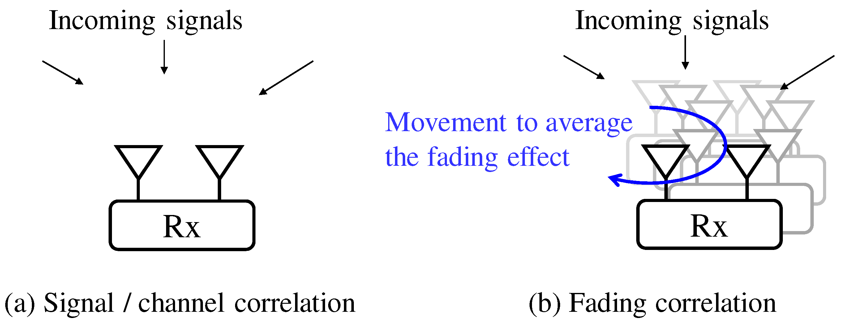
The fading correlation considers the representative characteristics of the environment. Figure 3 shows the concept of a method for obtaining the fading correlation characteristics. A MIMO channel is observed while moving an antenna array in the range defined as the area in which the distribution of incoming waves does not change. This aims to exclude fading variation in the environment in which the antenna is placed. However, if the antenna is moved too much, the number of incoming waves may vary due to shadowing, etc. Therefore, it is desirable that the range in which the antenna is moved be limited to just a couple of wavelengths.

The fading correlation matrix is defined by

$$\begin{array}{ccc}\hfill Receiverside:& {\mathit{R}}_R=& E\left[{\mathit{R}}_R^i\right]=E\left[\mathit{H}{\mathit{H}}^H\right]\hfill \end{array}$$

(11)

$$\begin{array}{ccc}\hfill Transmitterside:& {\mathit{R}}_T=& E\left[{\mathit{R}}_T^i\right]=E\left[{\mathit{H}}^H\mathit{H}\right].\hfill \end{array}$$

(12)

The correlation coefficients corresponding to Equations (11) and () are calculated by ${\rho }_{Rmn}=R_{Rmn}/\sqrt{R_{Rmm}{R}_{Rnn}}$ (between the m-th and n-th receiving antennas), ${\rho }_{Tpq}=R_{Tpq}/\sqrt{R_{Tpp}{R}_{Tqq}}$ (between the p-th and q-th transmitting antennas), respectively.

2.5. Complex Pattern Correlation

All the correlation matrices described so far contain both antenna and propagation characteristics. This section describes the correlation matrix that represents the antenna characteristics only. To examine the correlation of a MIMO antenna, its complex patterns (also called as ‘complex far-field patterns’ or ‘complex radiation patterns’) can be used. This defines a complex pattern correlation, which does not consider the propagation characteristics, i.e., the number of the arriving paths is sufficiently large and they distribute randomly in all directions (called as 3D uniform or Rayleigh environment). Note that the patterns dealt with in this paper are known as ‘array element pattern’ or ‘embedded element pattern’, where the array element pattern can be observed when one out of all antenna elements in the array is excited while other antennas are terminated by loads corresponding to the reference impedance (normally, it is 50 $\Omega$ including the internal resistance of the exciting source).

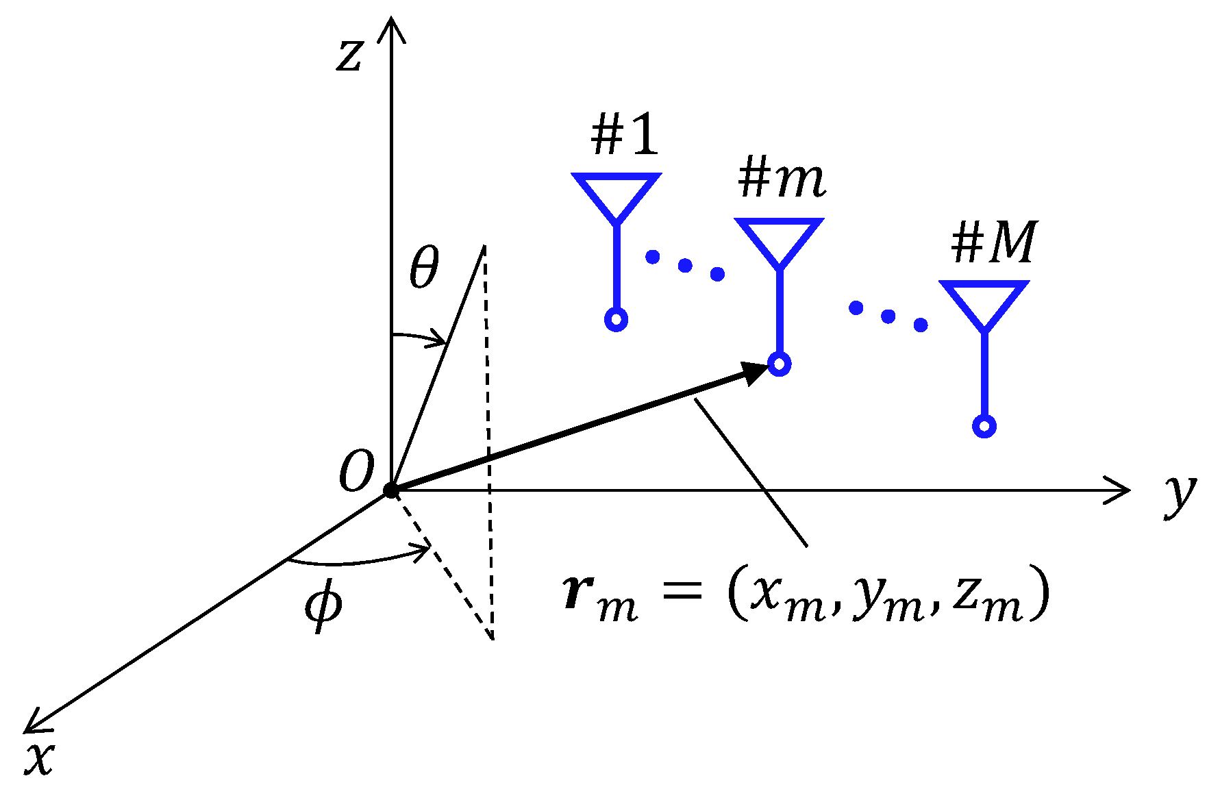
Figure 4 shows an M-element multi-antenna in a three-dimensional space. The complex pattern of the m-th antenna is defined as

$$\begin{array}{c}\hfill {\mathit{D}}_{0m}(\theta ,\varphi )=\left(\begin{array}{c}{D}_{\theta 0m}(\theta ,\varphi )\\ D_{\varphi 0m}(\theta ,\varphi )\end{array}\right).\end{array}$$

(13)

$D_{\theta 0m}(\theta ,\varphi )$ and $D_{\varphi 0m}(\theta ,\varphi )$ represent the complex gains of $\theta$ and $\varphi$ components, respectively. Note that $|D_{\theta 0m}{(\theta ,\varphi )|}^2$ and $|D_{\varphi 0m}{(\theta ,\varphi )|}^2$ correspond to the realized gain of antenna. ${\mathit{D}}_{0m}(\theta ,\varphi )$ is the 2D complex pattern of the m-th antenna elements when both of the antenna element’s centers (for example, feed point) and reference point are located at the origin point. When this antenna is moved to point ${\mathit{r}}_m=(x_m,y_m,z_m)$, the 2D complex pattern of the m-th antenna elements is expressed as

$$\begin{array}{c}\hfill {\mathit{D}}_m(\theta ,\varphi )=exp\{jk{\mathit{r}}_m·\mathit{e}(\theta ,\varphi )\}{\mathit{D}}_{0m}(\theta ,\varphi ),\end{array}$$

(14)

where k is a wave number and $\mathit{e}(\theta ,\varphi )$ is a unit vector corresponding to the observation direction; it is defined as $\mathit{e}(\theta ,\varphi )={(sin\theta cos\varphi ,sin\theta sin\varphi ,cos\theta )}^T$. In most MIMO antenna evaluations, the common reference point for all antenna elements is used as in Equation (14) for convenience. This means that the location of the antenna elements is explained by the phase information in the complex pattern. By using these complex patterns, the correlation matrix is defined as

$$\begin{array}{c}\hfill {\mathit{R}}_P=\frac{1}{4\pi }\int \int \left(\begin{array}{ccc}{\mathit{D}}_1^{*}{\mathit{D}}_1& \cdots & {\mathit{D}}_1^{*}{\mathit{D}}_M\\ ⋮& \ddots \\ {\mathit{D}}_M^{*}{\mathit{D}}_1& \cdots & {\mathit{D}}_M^{*}{\mathit{D}}_M\end{array}\right)d\Omega ,\end{array}$$

(15)

where $\Omega$ is the solid angle of observation defined as $d\Omega =sin\theta d\varphi d\theta$. In addition, the correlation coefficient is calculated as ${\rho }_{Pmn}=R_{Pmn}/\sqrt{R_{Pmm}{R}_{Pnn}}$, where m and n are the antenna numbers of interest, and $R_{Pmn}$ represents the m-th row and n-th column entry of the complex pattern correlation matrix shown in Equation (15).

2.6. S-Parameter Based Correlation

Section 2.5 explained the evaluation method of the correlation coefficient using the complex patterns. 2D radiation patterns have been generally used to evaluate the antenna efficiency or directivity, but most cases have used amplitude patterns (for example, [21,22,23]). If 2D complex patterns can be quickly measured, it becomes easy to evaluate the performance of a MIMO antenna. However, measuring a full 2D pattern normally incurs a significant measurement time or equipment costs.

Fortunately, S-parameters are much easier to measure than the radiation patterns [9,14]. The S-parameter matrix contains only reflection and mutual coupling information while it does not directly represent radiation properties. Nevertheless, the pattern correlations can be calculated from just the S-parameter matrix conditionally [8]. However, the radiation efficiency excluding reflection and mutual coupling losses must be close to 100%, that is, the Joule heat loss must be almost 0.

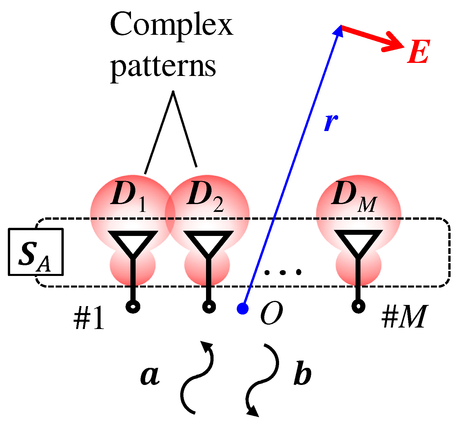
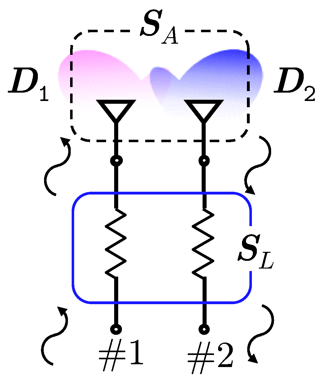
We now assume an antenna array whose S-parameter matrix is ${\mathit{S}}_A$ as shown in Figure 5. The signal, $\mathit{a}={(a_1,\dots ,a_M)}^T$, incidents the feed ports of the antenna array. The reflected signal vector is expressed as $\mathit{b}={\mathit{S}}_A\mathit{a}$. When the complex pattern of the m-th antenna element is expressed as ${\mathit{D}}_m$, the observed field generated by this antenna array at a sufficiently distant point is expressed as

$$\begin{array}{c}\hfill \mathit{E}=\sqrt{\frac{{\eta }_0}{4\pi }}({\mathit{D}}_1,\dots ,{\mathit{D}}_M)\mathit{a}\frac{e^{-jkr}}{r},\end{array}$$

(16)

where ${\eta }_0$ is the characteristic impedance of vacuum and r is the distance between the observation and reference points. By using (16), the total radiated power is expressed as

$$\begin{array}{c}\hfill P_{rad}=\frac{1}{{\eta }_0}\int \int {\mathit{E}}^H\mathit{E}d\Omega \end{array}$$

$$\begin{array}{cc}=& {\mathit{a}}^H\left[\frac{1}{4\pi }\int \int {({\mathit{D}}_1,\dots ,{\mathit{D}}_M)}^H({\mathit{D}}_1,\dots ,{\mathit{D}}_M)d\Omega \right]\mathit{a}\hfill \\ =& {\mathit{a}}^H\left[\frac{1}{4\pi }\int \int \left(\begin{array}{ccc}{\mathit{D}}_1^{*}{\mathit{D}}_1& \cdots & {\mathit{D}}_1^{*}{\mathit{D}}_M\\ ⋮& \ddots & \\ {\mathit{D}}_M^{*}{\mathit{D}}_1& \cdots & {\mathit{D}}_M^{*}{\mathit{D}}_M\end{array}\right)d\Omega \right]\mathit{a}.\hfill \end{array}$$

(17)

By substituting (15) into (17), the total radiated power is given by

$$\begin{array}{c}\hfill P_{rad}={\mathit{a}}^H{\mathit{R}}_P\mathit{a}.\end{array}$$

(18)

Meanwhile, if the antenna is lossless (no dielectric loss and no conductor loss), the total radiated power should agree with the total input power, which is defined by the incident power minus reflected power. This relation is represented by

$$\begin{array}{c}\hfill P_{rad}={\mathit{a}}^H\mathit{a}-{\mathit{b}}^H\mathit{b}={\mathit{a}}^H(\mathit{I}-{\mathit{S}}_A^H{\mathit{S}}_A)\mathit{a}.\end{array}$$

(19)

Comparing (18) to (19) yields the interesting relation,

$$\begin{array}{c}\hfill {\mathit{R}}_P=\mathit{I}-{\mathit{S}}_A^H{\mathit{S}}_A.\end{array}$$

(20)

This indicates that the correlation characteristics can be calculated from the S-parameter matrix only when the antenna array is lossless. In the following, the S-parameter based correlation matrix is expressed by ${\mathit{R}}_S$ to distinguish it from the complex pattern correlation matrix, ${\mathit{R}}_P$. The complex correlation coefficient between the p-th and q-th antenna elements is calculated as

$$\begin{array}{ccc}\hfill {\rho }_{Spq}& =& \frac{R_{Spq}}{\sqrt{R_{Spp}{R}_{Sqq}}}\hfill \\ & =& \frac{{\displaystyle -\sum _{m=1}^M{s}_{mq}^{*}{s}_{mp}}}{\sqrt{{\displaystyle 1-\sum _{m=1}^M{\left|s_{mp}\right|}^2}}\sqrt{{\displaystyle 1-\sum _{m=1}^M{\left|s_{mq}\right|}^2}}},\hfill \end{array}$$

(21)

where $R_{Spq}$ represents the p-th row and q-th column entry of ${\mathit{R}}_S$ and $s_{pq}$ represents the p-th row and q-th column entry of ${\mathit{S}}_A$.

2.7. Summary of the Various Kinds of Correlation Definitions

Table 1. Definitions of the correlation matrices.

$\mathbf{Name}$	Definition	Meaning
Signal correlation	${\mathit{R}}_{yy}=E\left[\mathit{y}\left(t\right){\mathit{y}}^H\left(t\right)\right]$	Correlation characteristics of the complex signal vector, $\mathit{y}\left(t\right)$
Channel correlation	$\begin{array}{l}{\mathit{R}}_R^i={\mathit{HH}}^H\left(Receiver\right)\\ {\mathit{R}}_T^i={\mathit{H}}^H\mathit{H}\left(Transmitter\right)\end{array}$	$\begin{array}{c}\mathrm{Instantaneous} \mathrm{correlation}\\ \mathrm{of} \mathrm{the} \mathrm{channel} \mathrm{between}\\ 2 \mathrm{fixed} \mathrm{locations}\end{array}$
Fading correlation	$\begin{array}{c}{\mathit{R}}_R=E\left[{\mathit{R}}_R^i\right]=E\left[{\mathit{HH}}^H\right]\left(\mathrm{Receiver}\right)\\ {\mathit{R}}_T=E\left[{\mathit{R}}_T^i\right]=E\left[{\mathit{H}}^H\mathit{H}\right]\left(\mathrm{Transmitter}\right)\end{array}$	Statistical correlation of the certain environment
Complex pattern correlation	$\begin{array}{c}{\displaystyle {\mathit{R}}_P=\frac{1}{4\pi }\int \int \left(\begin{array}{ccc}{\mathit{D}}_1^{*}{\mathit{D}}_1& \cdots & {\mathit{D}}_1^{*}{\mathit{D}}_M\\ ⋮& \ddots \\ {\mathit{D}}_M^{*}{\mathit{D}}_1& \cdots & {\mathit{D}}_M^{*}{\mathit{D}}_M\end{array}\right)d\Omega }\end{array}$	Correlation computed from complex pattern functions
S-parameter based correlation	${\mathit{R}}_S=\mathit{I}-{\mathit{S}}_A^H{\mathit{S}}_A$	${\mathit{R}}_P={\mathit{R}}_S$ (Valid only when Joule heat loss is 0)

summarizes the above mentioned spatial correlation matrices and their definitions. Note that all of them, other than ${\mathit{R}}_{yy}$, are spatial correlation matrices. The signal correlation matrix is calculated from the signal vector $\mathit{y}\left(t\right)$ observed by the antenna, and several hundreds or thousands of snapshots (number of samples during the observation period) are usually required to obtain ${\mathit{R}}_{yy}$ accurately. The channel correlation matrix is calculated from just the channel information between transmitting and receiving antennas at fixed points, and represents the instantaneous channel characteristics, where it is equivalent to the environment wherein the channel is completely static. Note that it is calculated only when the channel between transmitting and receiving antennas can be estimated. Fortunately, this is not difficult to obtain because most MIMO systems perform channel estimation. When noise is ignored and signal strength is normalized, ${\mathit{R}}_R^i={\mathit{R}}_{yy}$ is satisfied.

The fading correlation matrix is obtained by averaging the channel correlation matrix over the frequency band or locations of transmitting/receiving antennas (the relative position of the antenna in the antenna array must not be changed) in a certain environment [24,25,26]. Generally speaking, the term ‘spatial correlation matrix’ refers to this fading correlation matrix [24]. In addition, the fading correlation matrix is equal to the complex pattern correlation matrix only when the angular distribution of the departure and arrival paths are 3D uniform if the number of the paths is sufficiently large. The S-parameter correlation matrix is equal to the complex pattern correlation matrix if the Joule heat loss is zero [8], and also equal to the normalized fading correlation matrix with the 3D-uniform environment as described above.

The fading correlation matrix is applicable to the Kronecker model, which is commonly used to compute MIMO channels [6,27]. Moreover, the complex pattern and S-parameter-based correlation matrices can also be used for the Kronecker model. Note that the channel correlation matrix cannot be used for the Kronecker model because this correlation considers only the instantaneous channel characteristics, which do not necessarily represent the statistical properties of the environment.

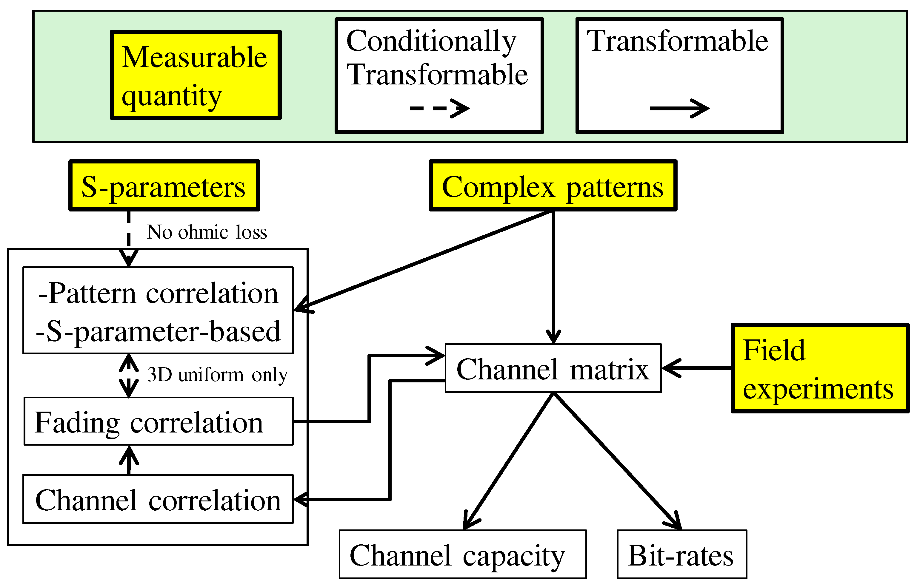
Figure 6 shows the relationship among the measurable and computable quantities through the correlation characteristics. The complex pattern is quite useful information because this can yield various kinds of the physical quantities that are used in MIMO systems. For example, the channel matrix is directly computed by combining the complex patterns and various kinds of channel models like GSCM. The complex ‘pattern correlation’ matrix can be computed from the complex patterns, and is identical to the ‘fading correlation’ matrix given the assumption of a 3D uniform environment. The ‘S-parameter-based’ correlation matrix is computed from the S-parameter matrix, and is identical to the complex pattern correlation matrix if the radiation efficiency of the antenna array is 100%. The fading correlation can yield the channel matrix by using a channel model like the Kronecker model. The instantaneous ‘channel correlation’ is directly calculated from the channel matrix, and the fading correlation is also computed again by averaging the instantaneous channel correlation over several hundreds or thousands of snapshots. Field experiments are effective in confirming the real channel matrix, but it is difficult to separate the antenna and environmental characteristics.

3. Simulation

As mentioned above, the signal correlation matrix and channel correlation matrix are fundamentally identical if the signal-to-noise ratio is sufficiently high, and their correlation characteristics are easily simulated and measured.

The remaining three correlation characteristics are strongly related, while their similarity is vulnerable to the environment and antenna efficiency. Therefore, the correlation coefficients to be compared here are the fading correlation matrix shown in (11), the complex pattern correlation matrix as in (15), and the S-parameter based correlation matrix as in (20). To assess the impact of the antenna characteristics on these three correlation characteristics, a Rayleigh environment is assumed, where the sufficient numbers of paths distribute uniformly in all directions. In addition, the fading correlation is evaluated only at the receiver side for simplicity.

3.1. Antenna and Channel Models

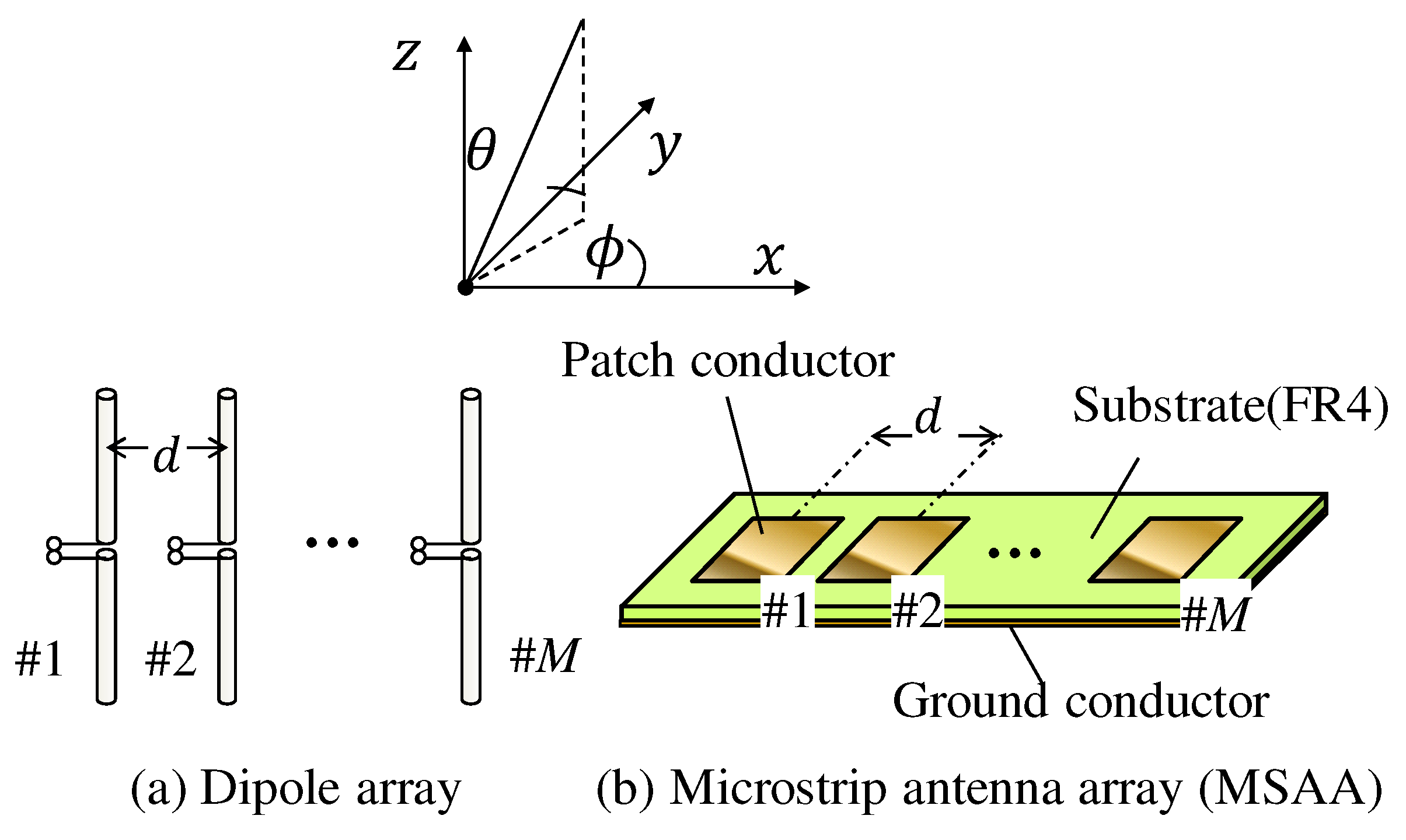
Two kinds of antenna arrays are dealt with in this paper, and the correlation coefficient is varied by changing the element spacing. Figure 7 shows the antenna models. Here, (a) is a half-wavelength dipole array and (b) is a square microstrip antenna array (MSAA); both are linear arrays with element intervals of d in the H-plane. The size of the conductor-backed dielectric substrate of (b) is determined so that the distance between the substrate edge and the center of each antenna element is 0.5 wavelengths. The thickness of the dielectric substrate was 1.6 mm, the relative dielectric constant was 4.2, and the dielectric loss tangent was 0.02. Both the dipole and MSAA had an operating frequency of 2.4 GHz. The moment-method based simulator (HyperLynx 3D EM) was used.

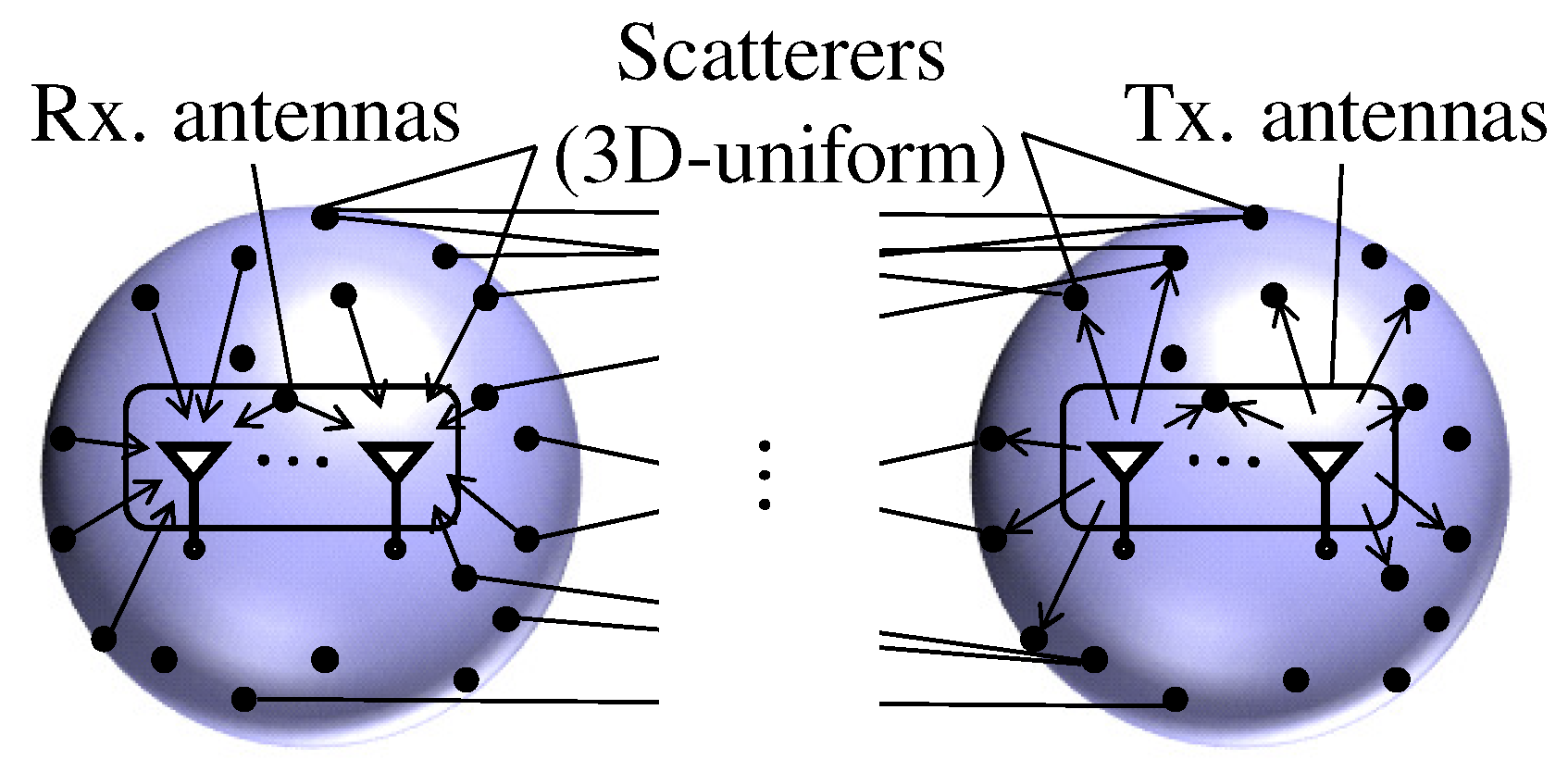
Figure 8 is a conceptual diagram of the model used to compute the propagation channel. This is a geometry-based stochastic channel model (GSCM) [7], and well explains the physical path distributions around the antennas. The scatterers are arranged sufficiently far from each antenna. Each entry of the MIMO channel matrix is yielded by the sum of all element paths from one of the transmitting antennas to one of the receiving antennas. In this simulation, the statistical conditions of the environment are identical for both transmitting and receiving sides. The number of the scatterers is set to 100 for each side, and the distribution of the scatterers are set to 3D uniform. The propagation channel is generated 1000 times for each antenna condition, where identical antenna arrays are used for both sides. The GSCM model is used only to calculate the fading correlation matrix. This is because both the complex pattern and S-parameter-based correlation matrices are determined by the antenna characteristics only, while the fading correlation matrix needs the propagation channel.

3.2. Results

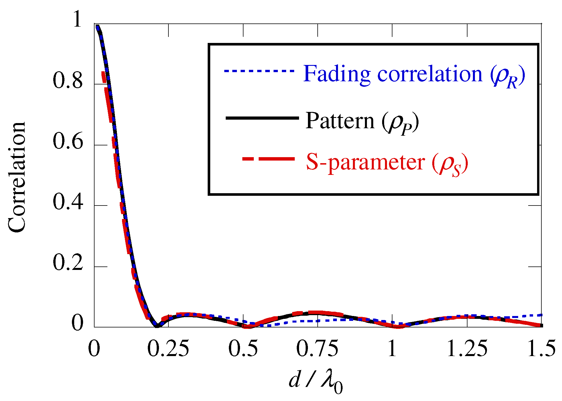
Figure 9 plots the correlation coefficient versus the element spacing of a dipole array ($M=2$), where ${\lambda }_0$ represents the wavelength in a vacuum. These results show that the correlation coefficients obtained by the three calculation methods almost agree. When the element spacing is wide, the fading correlation calculated by the GSCM diverges from those of the other methods. This is considered to be caused by insufficient resolution ($\theta$ Direction: $5^{\circ }$, $\varphi$Direction: ${10}^{\circ }$) of the complex pattern used in the scattering ring model.

Figure 10 shows the element spacing characteristics of the correlation coefficient for the dipole array ($M=4$). Since the structure is bilaterally symmetric, the correlation coefficients, which are identical in principle, are shown jointly. As a result, it was found that all methods yielded almost the same correlation coefficients. However, when S-parameter was used, the estimated correlation coefficient was slightly lower when the element interval was narrow. It is considered that the radiation efficiency (excluding reflection and coupling loss) was degraded by the effect of conductor loss because the finite conductivity (${\sigma }_{Cu}=5.7\times {10}^7$ S/m) of copper was used.

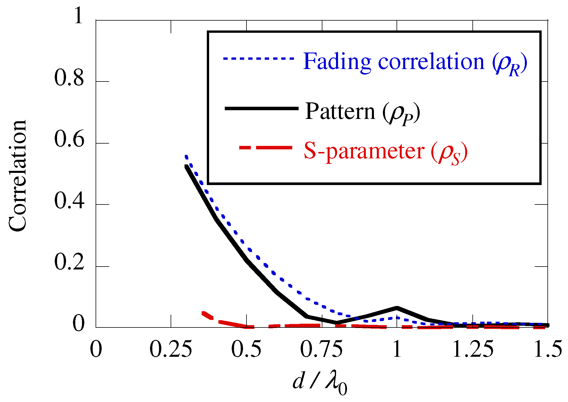
Since the radiation efficiency of the dipole array examined above is high, the correlation coefficients obtained by the three methods agreed well. Next, the accuracy of the correlation coefficients was compared using MSAA with dielectric loss. Figure 11 shows the result of the correlation coefficient of the 2-element MSAA. From this result, it is found that the complex pattern correlation given by (15) agrees well with the fading correlation by using GSCM, but the S-parameter-based correlation by (20) is always underestimated and diverges strongly from the others. This is because, when the loss is large, the radiation power of the antenna decreases, and, as a result, the mutual coupling between the antennas tends to decrease. Thus, the correlation coefficient using S-parameters is inaccurate for lossy antennas. The radiation efficiency, in this case, was about $33\%$ when the element spacing was $0.3{\lambda }_0$, and about $39\%$ when the element spacing was greater than $0.5{\lambda }_0$.

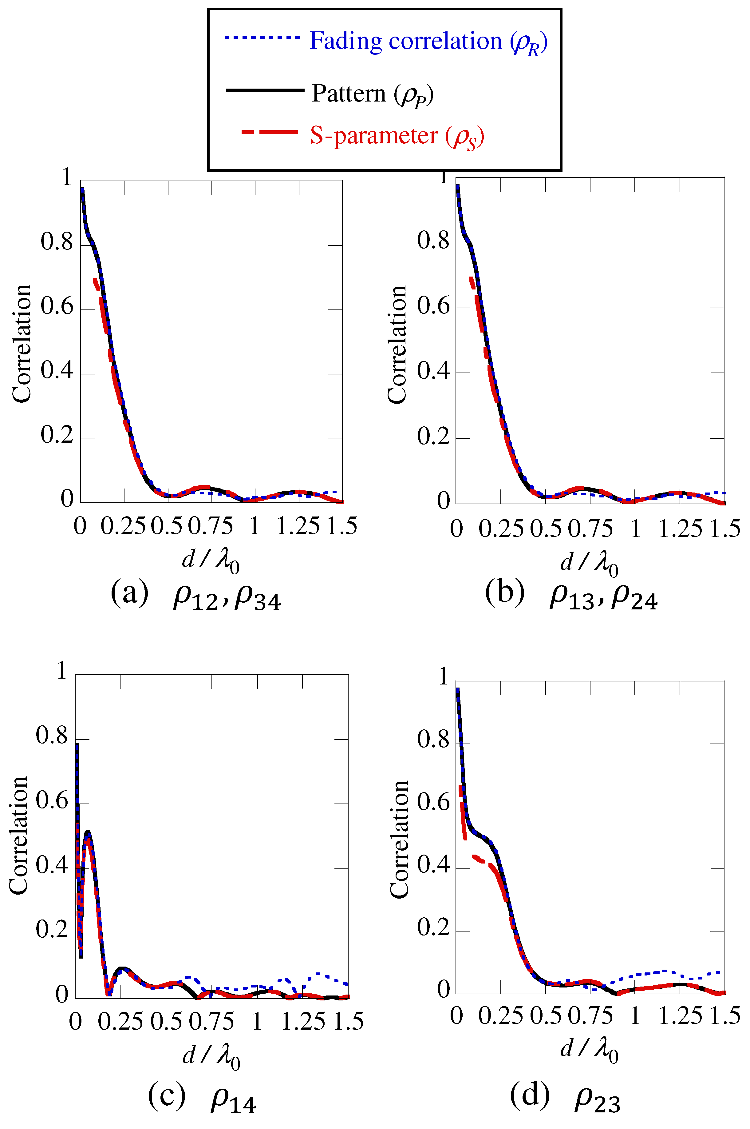
Figure 12 shows the correlation coefficient of the 4-element MSAA. The S-parameter based correlation yielded by (20) diverges significantly from those of the other methods. Similarly, the radiation efficiency is about 27% to 40%, which seriously degrades the accuracy of the S-parameter based correlation coefficient.

To confirm the impact of the radiation efficiency on the accuracy of the S-parameter based correlation coefficient, the lossy dipole model is analyzed; resistive attenuators are intentionally inserted at the feed port. Figure 13 shows the model of the lossy dipole array, where the dipole antenna elements are the same as those in Figure 7. The antenna S-parameter matrix, which has a loss term due to attenuator insertion, is expressed as

$$\begin{array}{c}\hfill {\mathit{S}}^{\prime }={\mathit{S}}_{L12}{\mathit{S}}_A{\mathit{S}}_{L21}=\eta {\mathit{S}}_A\end{array}$$

(22)

where $\eta$ is radiation efficiency ($0\le \eta \le 1$), and ${\mathit{S}}_{L12}={\mathit{S}}_{L21}={\eta }^{1/2}\mathit{I}$. Equation (22) is correct only if the antenna element is lossless and the attenuator is fully matched. Since reflection does not occur in the attenuator circuit, its S-parameter matrix is expressed as

$$\begin{array}{c}\hfill {\mathit{S}}_L=\left(\begin{array}{cc}\mathit{0}& {\mathit{S}}_{L12}\\ {\mathit{S}}_{L21}& \mathit{0}\end{array}\right).\end{array}$$

(23)

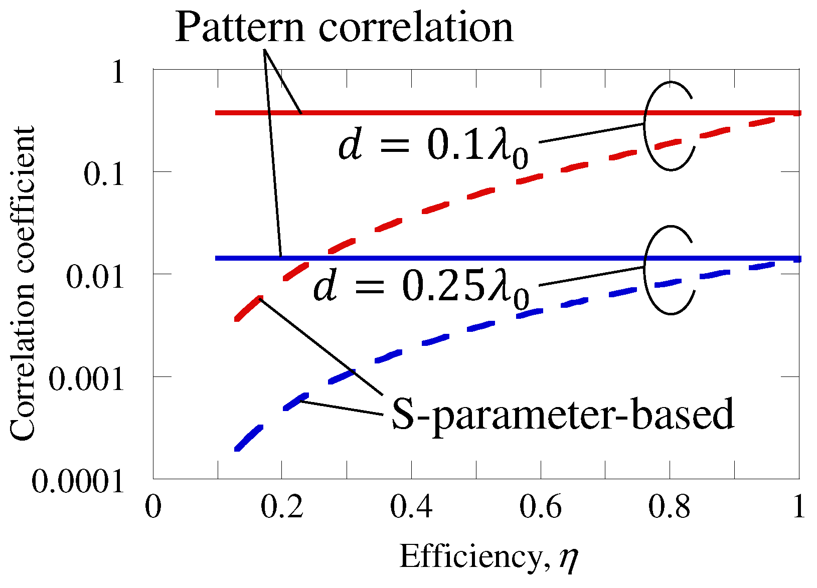
Figure 14 shows the simulated relationship between the correlation coefficients and radiation efficiency $\eta$. It can be seen the S-parameter-based correlation coefficient falls as $\eta$ becomes low. It is found that the antenna even with the efficiency higher than 97% radiation efficiency yields correlation coefficient errors of up to 10%. This means that the S-parameter based correlation coefficient is quite unreliable for most practical compact antennas.

To circumvent this problem, some methods for correcting the correlation coefficient by considering the radiation efficiency have been studied (for example, [13]). However, it is necessary to choose the right correction method to suit the location at which the loss occurs in the antenna. This means it is difficult to apply these correction methods to all kinds of antennas without knowing the detailed antenna’s current distributions.

4. Conclusions

In this paper, the current definitions of the correlation coefficient of MIMO antennas have been explained. Numerical calculations were introduced to examine the effect of element spacing and type on the accuracy of the correlation coefficients. In particular, a numerical analysis of the 2-element dipole array showed that the S-parameter-based correlation yields an error greater than 10% if the radiation efficiency is lower than 97%, and this means that most of the practical compact antennas cannot be evaluated by using the S-parameter-based correlation approach.

References

- Teletar, I.E. Capacity of Multi-Antenna Gaussian Channels; Tech. Rep.; AT&T-Bell Labs: Murray Hill, NJ, USA, 1995. [Google Scholar]
- Foschini, G.J.; Gans, M.J. Capacity when using diversity at transmit and receive sites and the Rayleigh-faded matrix channel is unknown at the transmitter. In Proceedings of the WINLAB Workshop on Wireless Information Network, New Brunswick, NJ, USA, 20–21 March 1996. [Google Scholar]
- Clarke, R. A statistical theory of mobile-radio reception. Bell Syst. Tech. J. 1968, 47, 957–1000. [Google Scholar] [CrossRef]
- Lee, W. Effects on correlation between two mobile radio base-station antennas. IEEE Trans. Commun. 1973, 21, 1214–1224. [Google Scholar] [CrossRef]
- Shiu, D.S.; Foschini, G.J.; Gans, M.J.; Kahn, J.M. Fading correlation and its effect on the capacity of multielement antenna systems. IEEE Trans. Commun. 2000, 48, 502–513. [Google Scholar] [CrossRef] [Green Version]
- Chizhik, D.; Rashid-Farrokhi, F.; Ling, J.; Lozano, A. Effect of antenna separation on the capacity of BLAST in correlated channels. IEEE Commun. Lett. 2000, 4, 337–339. [Google Scholar] [CrossRef]
- Molisch, A.F. A generic model for MIMO wireless propagation channels. IEEE Trans. Signal Process. 2004, 52, 61–71. [Google Scholar] [CrossRef]
- Blanch, S.; Romeu, J.; Corbella, I. Exact representation of antenna system diversity performance from input parameter description. Electron. Lett. 2003, 39, 705–707. [Google Scholar] [CrossRef] [Green Version]
- Nadeem, I.; Choi, D. Study on mutual coupling reduction technique for MIMO antennas. IEEE Access 2019, 7, 563–586. [Google Scholar] [CrossRef]
- Ludwig, A. Mutual coupling, gain and directivity of an array of two identical antennas. IEEE Trans. Antennas Propag. 1976, 24, 837–841. [Google Scholar] [CrossRef]
- Hallbjorner, P. The significance of radiation efficiencies when using S-parameters to calculate the received signal correlation from two antennas. IEEE Antennas Wirel. Propag. Lett. 2005, 4, 97–99. [Google Scholar] [CrossRef]
- Narbudowicz, A.; Ammann, M.J.; Heberling, D. Impact of lossy feed on S-parameter based envelope correlation coefficient. In Proceedings of the 2016 10th European Conference on Antennas and Propagation (EuCAP 2016), Davos, Switzerland, 10–15 April 2016. [Google Scholar]
- Li, H.; Lin, X.; Lau, B.K.; He, S. Equivalent circuit based calculation of signal correlation in lossy MIMO antennas. IEEE Trans. Antennas Propagat. 2013, 61, 5214–5222. [Google Scholar] [CrossRef] [Green Version]
- Sharawi, M.S.; Hassen, A.T.; Khan, M.U. Correlation coefficient calculations for MIMO antenna systems: A comparative study. Int. J. Microw. Wirel. Technol. 2017, 9, 1991–2004. [Google Scholar] [CrossRef]
- Kyritsi, P.; Chizhik, D. Capacity of multiple antenna systems in free space and above perfect ground. IEEE Commun. Lett. 2002, 6, 325–327. [Google Scholar] [CrossRef]
- Mao, C.; Chu, Q. Compact coradiator UWB-MIMO antenna with dual polarization. IEEE Trans. Antennas Propag. 2014, 62, 4474–4480. [Google Scholar] [CrossRef]
- Getu, B.; Andersen, J. The MIMO cube - a compact MIMO antenna. IEEE Trans. Wirel. Commun. 2005, 4, 1136–1141. [Google Scholar] [CrossRef]
- Das, N.K.; Inoue, T.; Taniguchi, T.; Karasawa, Y. An experiment on MIMO system having three orthogonal polarization diversity branches in multipath-rich environment. IEEE Veh. Technol. Conf. Fall 2004, 2, 1528–1532. [Google Scholar]
- Honma, N.; Nishimori, K.; Takatori, Y.; Ohta, A.; Tsunekawa, K. Proposal of compact three-port MIMO antenna employing modified inverted F antenna and notch antennas. In Proceedings of the 2006 IEEE International Symposium on Antennas and Propagation (AP-S 2006), Albuquerque, NM, USA, 9–14 July 2006; pp. 2613–2616. [Google Scholar]
- Wallace, J.W.; Jensen, M.A. Mutual coupling in MIMO wireless systems: A rigorous network theory analysis. IEEE Trans. Wirel. Commun. 2004, 3, 1317–1325. [Google Scholar] [CrossRef] [Green Version]
- Karlsson, A. On the efficiency and gain of antennas. Prog. Electromagn. Res. 2013, 136, 479–494. [Google Scholar] [CrossRef] [Green Version]
- Singh, P.K.; Saini, J. Effect of superstrate on a cylindrical microstrip antenna. Prog. Electromagn. Res. Lett. 2018, 75, 83–89. [Google Scholar] [CrossRef] [Green Version]
- Ndip, I.; Lang, K.D.; Reichl, H.; Henke, H. On the radiation characteristics of full-Loop, half-loop, and quasi-half-loop bond wire antennas. IEEE Trans. Antennas Propag. 2018, 66, 5672–5686. [Google Scholar] [CrossRef]
- Ivrlac, M.T.; Utschick, W.; Nossek, J.A. Fading correlations in wireless MIMO communication systems. IEEE J. Sel. Areas Commun. 2003, 21, 819–828. [Google Scholar] [CrossRef]
- Nishimoto, H.; Ogawa, Y.; Nishimura, T.; Ohgane, T. Measurement-based performance evaluation of MIMO spatial multiplexing in a multipath-rich indoor environment. IEEE Trans. Antennas Propag. 2017, 55, 3677–3689. [Google Scholar] [CrossRef] [Green Version]
- Nishimori, K.; Tachikawa, N.; Takatori, Y.; Kudo, R.; Tsunekawa, K. Frequency correlation characteristics due to antenna configurations in broadband MIMO transmission. IEICE Trans. Commun. 2005, E88-B, 2438–2445. [Google Scholar] [CrossRef]
- Oestges, C. Validity of the Kronecker model for MIMO correlated channels. In Proceedings of the 63rd IEEE Vehicular Technology Conference (VTC Spring), Melbourne, Australia, 7–10 May 2006; Volume 6, pp. 2818–2822. [Google Scholar]
Figure 1.
Impact of the antenna factors on correlation characteristics.
Figure 2.
Signal model of the MIMO antenna system.
Figure 3.
Method to observe fading correlation.
Figure 4.
Multiple antennas in the three-dimensionally defined space.
Figure 5.
Lossless antenna array excited by .
Figure 6.
Measurable quantities and yielded information.
Figure 7.
Antenna model.
Figure 8.
Conceptual sketch of GSCM.
Figure 9.
Correlation coefficient versus element spacing d: dipole array().
Figure 10.
Figure 11.
Correlation coefficient versus element spacing d: MSAA ().
Figure 12.
Figure 13.
Lossy dipole array model ().
Figure 14.
Correlation coefficient versus radiation efficiency : dipole array ().