Inversion-Based Approach for Detection and Isolation of Faults in Switched Linear Systems

Abstract

This paper addresses the problem of the left inversion of switched linear systems from a diagnostics perspective. The problem of left inversion is to reconstruct the input of a system with the knowledge of its output, whose differentiation is usually required. In the case of this work, the objective is to reconstruct the system’s unknown inputs, based on the knowledge of its outputs, switching sequence and known inputs. With the inverse model of the switched linear system, a real-time Fault Detection and Isolation (FDI) algorithm with an integrated Fuzzy Logic System (FLS) that is capable of detecting and isolating abrupt faults occurring in the system is developed. In order to attenuate the effects of unknown disturbances and noise at the output of the inverse model, a smoothing strategy is also used. The results are illustrated with an example. The performance of the method is validated experimentally in a dc-dc boost converter, using a low-cost microcontroller, without any additional components.

1. Introduction

The problem of linear systems inversion is a concept that gathered great interest among the control engineering community since the middle of last century. The inversion of Multiple-Input Multiple-Output (MIMO) state-space systems was principally driven by Reference [1,2] which gave, with their contributions, a lot of insight into the comprehension of the properties of inverse systems. The former, realized with his so-called structure algorithm, that an inverse system can be achieved with the same number of differentiators (or delay elements) as the original system. The latter studied principally left inversions and introduced the concept of inherent integration (delay) of continuous (discrete) Linear Time-Invariant (LTI) systems.

Some years later, Reference [3] provided necessary and sufficient conditions for the stable invertibility and introduced the concepts of left and right inverses. In fact, regarding its application, the problem of inversion can be divided into two classes—(i) right inversion; and (ii) left inversion. While right inversion deals with finding inputs and initial conditions that produce a given output, left inversion is related with the problem of recovering unknown inputs applied to the system from the knowledge of its outputs. As stated by Reference [3], a left inverse for a system $\mathbf{\Sigma }$ is a system ${\mathbf{\Sigma }}^{\mathsf{L}}$ which computes the input to $\mathbf{\Sigma }$ from the knowledge of its output, such that ${\mathbf{\Sigma }}^{\mathsf{L}}\mathbf{\Sigma }={\mathit{I}}_m$. One can verify if a system is left invertible by the following definition:

Definition 1

(Left Invertibility). Let $u_1$ and $u_2$ be any two inputs to system Σ and let $y_1$ and $y_2$ be the corresponding outputs for the same initial state. System Σ is said to be left invertible if $y_1\left(t\right)=y_2\left(t\right)$ for all $t\ge 0$ implies that $u_1\left(t\right)=u_2\left(t\right)$ for all $t\ge 0$.

Whilst right inversion deals typically with reference tracking in control applications, an important domain of application for the left inversion problem is the one related to model-based Fault Detection and Isolation (FDI) [4,5].

Hence, the inversion of linear systems plays an important role not only in the areas of digital signal processing [6] and control systems [7,8], but also in the area of fault diagnosis [9,10,11,12]. In these latter works, it were explored different approaches to take advantage of the concept of system inversion to tackle the problem of FDI, specially in the linear case. Although there is a close link between input observability and system inversion, the first is preferred when addressing the problem of input reconstruction [13]. Nevertheless, the concept of left inversion has been widely used by the scientific community for unknown input reconstruction [8,10,12,13,14,15]. Basically, the idea is to model faults as unknown inputs and to invert the system to reconstruct them.

Since power electronics converters are embedded in almost every modern electric and electronic application, there were published some works related to inversion of Switched Linear Systems (SLSs). The problem of invertibility of SLSs was introduced by Reference [16], where it was addressed the recovery of the switching signal and input from the knowledge of the output and initial state. In their work, they gave the necessary and sufficient conditions for a switched system to be invertible, based on the methodology of inversion proposed by Reference [1] for LTI systems. This algorithm was already adapted for the purpose of accomplish FDI for the case of LTI systems [17,18] and also for the case of switched linear systems using state-space approaches [19]. Giving some continuity to his work, Reference [20] addressed the invertibility problem for switched nonlinear systems. Both of these works were developed from a perspective of control.

Regarding the approach proposed by Reference [2], there are only a few works using it with the purpose of FDI, for example, References [21,22]. Hence, the goal of this paper is twofold. Firstly, the article provides a detailed perspective on the state-space inversion approach, developed based on the work of Sain and Massey [2], for researchers who are familiar with FDI, showing the mathematical explanations and formal proofs. Secondly, the problem of inversion of Switched Linear Systems is introduced to a wide audience, guiding practicing engineers in the field to a new solution to their FDI problems for SLSs.

2. General Setting of the FDI Approach and Previous Results

In this section, we set up the problem and review our previous results. As referred before, the concept of left inversion is close related to fault diagnosis, since it permits to reconstruct the input of the original system from the knowledge of its output. Consequently, the concept can be adapted to reconstruct faults modeled as unknown inputs. Henceforth, the Sain and Massey’s [2] state-space inversion approach will be adapted to accommodate faults modeled as unknown inputs, which one are interested in recover. Moreover, this state-space mathematical description will be performed in discrete-time, since it has more advantages regarding its implementation in digital controllers. Consequently, the usual state-space description is replaced by a new one, where it is included an additional unknown input vector and its corresponding matrix.

Consider a system or process described by the following generalized discrete-time state-space dynamical model $\mathbf{\Gamma }$, with ${\mathit{x}}_0=\mathit{x}\left(0\right)=\mathbf{0}$:

$$\mathbf{\Gamma }=\{\begin{array}{}\mathrm{(1a)}& \hfill {\mathit{x}}_{k+1}& =& \mathit{A}{\mathit{x}}_k+\mathit{B}{\mathit{u}}_k+\mathit{F}{\mathit{\phi }}_k\hfill \mathrm{(1b)}& \hfill {\mathit{y}}_k& =& \mathit{C}{\mathit{x}}_k\hfill \end{array}$$

where $k\in \mathbb{N}$ is the natural number standing for the discrete time instant, ${\mathit{x}}_k=\mathit{x}\left(kT\right)\in {\mathbb{R}}^n$ is the state vector, ${\mathit{u}}_k\in {\mathbb{R}}^m$ is the known input vector, ${\mathit{\phi }}_k\in {\mathbb{R}}^{\ell }$ is the unknown input vector, and ${\mathit{y}}_k\in {\mathbb{R}}^p$ is the output vector. Moreover, $\mathit{A}\in {\mathbb{R}}^{n\times n}$, $\mathit{B}\in {\mathbb{R}}^{n\times m}$, $\mathit{C}\in {\mathbb{R}}^{p\times n}$ and $\mathit{F}\in {\mathbb{R}}^{n\times \ell }$ are the matrices that define system (1). As it is shown, the feed-through $\mathit{D}$ matrix is absent from (1b) since the majority of the modeled physical systems are strictly proper.

From (1), for any given integer $i\ge 0$, one can write its state sequence $\mathcal{X}=\left\{{\mathit{x}}_k, {\mathit{x}}_{k+1}, \dots , {\mathit{x}}_{k+i}\right\}$ over $i+1$ time-steps as:

$$\begin{array}{cc}\hfill {\mathit{x}}_k& ={\mathit{x}}_0\hfill \end{array}$$

(2a)

$$\begin{array}{cc}\hfill {\mathit{x}}_{k+i}& ={\mathit{A}}^i{\mathit{x}}_k+\sum _{j=0}^{i-1}{\mathit{A}}^{i-1-j}{\mathit{Bu}}_{k+j}+\sum _{j=0}^{i-1}{\mathit{A}}^{i-1-j}{\mathit{F}\mathit{\phi }}_{k+j},\hspace{1em}i=1,2,3,\dots ,\hfill \end{array}$$

(2b)

where $\mathcal{U}=\left\{{\mathit{u}}_k, {\mathit{u}}_{k+1}, \dots , {\mathit{u}}_{k+i-1}\right\}$ is the known input sequence and $\Phi =\left\{{\mathit{\phi }}_k, {\mathit{\phi }}_{k+1}, \dots , {\mathit{\phi }}_{k+i-1}\right\}$ is the unknown input sequence. In the same manner one can write the output sequence $\mathcal{Y}=\left\{{\mathit{y}}_k, {\mathit{y}}_{k+1}, \dots , {\mathit{y}}_{k+i}\right\}$ as:

$$\begin{array}{cc}\hfill {\mathit{y}}_k& ={\mathit{Cx}}_k\hfill \end{array}$$

(3a)

$$\begin{array}{cc}\hfill {\mathit{y}}_{k+i}& ={\mathit{CA}}^i{\mathit{x}}_k+\mathit{C}\sum _{j=0}^{i-1}{\mathit{A}}^{i-1-j}{\mathit{Bu}}_{k+j}+\mathit{C}\sum _{j=0}^{i-1}{\mathit{A}}^{i-1-j}{\mathit{F}\mathit{\phi }}_{k+j},\hspace{1em}i=1,2,3,\dots .\hfill \end{array}$$

(3b)

Hence, one are interested in recover the unknown input vector ${\mathit{\phi }}_k$ by inverting the system described by the state-space model (1), based on the approach developed initially by References Sain and Massey [2,23] for inverting LTI systems.

Accordingly, system $\mathbf{\Gamma }$ is invertible if it has an L-delay inverse for some finite L. The least integer L for which an L-delay inverse exists is called the inherent delay of the invertible system $\left(L_0\right)$. This inherent delay of the invertible system is the least number of differentiations required to recover the original system’s unknown input from the knowledge of its input and output. A consequence of not having $\mathit{D}$ matrix is that $L_0$ will be at least equal to one, since at least one differentiation will be required to reconstruct the unknown input vector ${\mathit{\phi }}_k$.

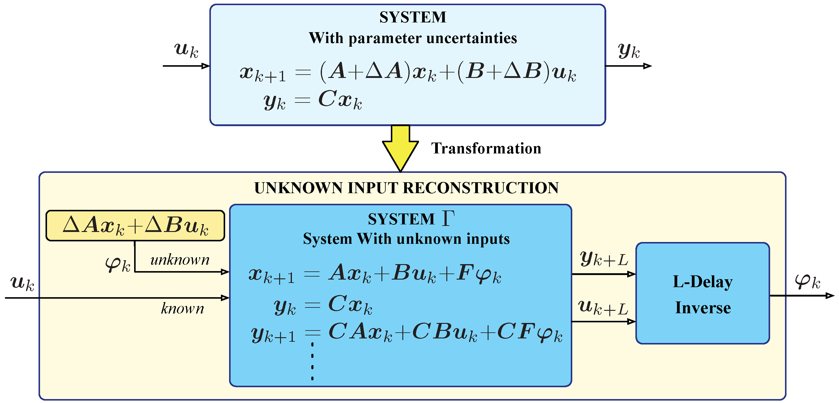
The referred concept of reconstructing an unknown input is depicted in Figure 1. On the top, it is shown the state-space description of a system, modeled with parameter uncertainties that affect both $\mathit{A}$ and $\mathit{B}$ matrices. This system is transformed to one that have these unknown parameter uncertainties modeled as unknown inputs. Since the output equation does not have any information from this vector, one need to perform some differentiations in order to subsequently recover it.

Then, the L-delay inverse block performs the inversion of the system and reconstructs the unknown input vector after L-delays. This L-delay inverse block will be shown in more detail afterwards. Note that, for $\mathbf{\Gamma }$ to have an L-delay inverse, the system must have at least as many outputs as unknown inputs, that is, $p\ge \ell$.

Imbued in this concept of input reconstruction, it is now necessary to adapt the Sain and Massey’s inversion algorithm proposed in Reference [2] to this new approach, that is, the system is modeled in discrete-time and there is a new unknown input vector which one want to reconstruct. This matrix $\mathit{F}$ and vector ${\mathit{\phi }}_k$ that are added to the state equation are the main challenges faced doing this adaptation.

Firstly, let ${\mathit{u}}_{[k:k+L-1]}\in {\mathbb{R}}^{mL}$, ${\mathit{\phi }}_{[k:k+L]}\in {\mathbb{R}}^{\ell L}$ and ${\mathit{y}}_{[k:k+L]}\in {\mathbb{R}}^{p(1+L)}$ denote the vectors of sequences over $L+1$ time units, for the known inputs, unknown inputs and outputs, respectively, which are given by:

${\mathit{y}}_{[k:k+L]}:=\left[\begin{array}{c}{\mathit{y}}_k\\ {\mathit{y}}_{k+1}\\ ⋮\\ {\mathit{y}}_{k+L}\end{array}\right]$, ${\mathit{u}}_{[k:k+L-1]}:=\left[\begin{array}{c}{\mathit{u}}_k\\ {\mathit{u}}_{k+1}\\ ⋮\\ {\mathit{u}}_{k+L-1}\end{array}\right]$ and ${\mathit{\phi }}_{[k:k+L-1]}:=\left[\begin{array}{c}{\mathit{\phi }}_k\\ {\mathit{\phi }}_{k+1}\\ ⋮\\ {\mathit{\phi }}_{k+L-1}\end{array}\right]$.

From (3), assuming known initial state (so that its effects can be subtracted out), it can readily be checked that:

$${\mathit{y}}_{[k:k+L]}={\mathcal{O}}_L{\mathit{x}}_k+{\mathcal{H}}_L{\mathit{u}}_{[k:k+L-1]}+{\mathcal{M}}_L{\mathit{\phi }}_{[k:k+L-1]},$$

(4)

where matrices ${\mathcal{O}}_L\in {\mathbb{R}}^{p(1+L)\times n}$, ${\mathcal{H}}_L\in {\mathbb{R}}^{p(1+L)\times mL}$ and ${\mathcal{M}}_L\in {\mathbb{R}}^{p(1+L)\times \ell L}$ can be defined recursively (neglecting the right $\mathbf{0}$ column) for $i\ge 1$ as:

$$\begin{array}{cc}\hfill {\mathcal{O}}_0& =\mathit{C}\hfill \end{array}$$

(5a)

$$\begin{array}{cc}\hfill {\mathcal{O}}_i& =\left[\begin{array}{c}\mathit{C}\\ {\mathcal{O}}_{i-1}\mathit{A}\end{array}\right],\hspace{1em}i=1,2,\dots \hfill \end{array}$$

(5b)

$$\begin{array}{cc}\hfill {\mathcal{O}}_i& =\left[\begin{array}{c}\mathit{C}\\ \mathit{CA}\\ ⋮\\ {\mathit{CA}}^i\end{array}\right],\hfill \end{array}$$

(5c)

$$\begin{array}{cc}\hfill {\mathcal{H}}_0& =\mathbf{0}\hfill \end{array}$$

(6a)

$$\begin{array}{cc}\hfill {\mathcal{H}}_i& =\left[\begin{array}{cc}\mathbf{0}& \mathbf{0}\\ {\mathcal{O}}_{i-1}\mathit{B}& {\mathcal{H}}_{i-1}\end{array}\right],\hspace{1em}i=1,2,\dots \hfill \end{array}$$

(6b)

$$\begin{array}{cc}\hfill {\mathcal{H}}_i& =\left[\begin{array}{ccccc}\mathbf{0}& \mathbf{0}& \mathbf{0}& \cdots & \mathbf{0}\\ \mathit{CB}& \mathbf{0}& \mathbf{0}& \cdots & \mathbf{0}\\ \mathit{CAB}& \mathit{CB}& \mathbf{0}& \cdots & \mathbf{0}\\ ⋮& ⋮& ⋮& \ddots & ⋮\\ {\mathit{CA}}^{i-1}\mathit{B}& {\mathit{CA}}^{i-2}\mathit{B}& {\mathit{CA}}^{i-3}\mathit{B}& \cdots & \mathit{CB}\end{array}\right],\hfill \end{array}$$

(6c)

and

$$\begin{array}{cc}\hfill {\mathcal{M}}_0& =\mathbf{0}\hfill \end{array}$$

(7a)

$$\begin{array}{cc}\hfill {\mathcal{M}}_i& =\left[\begin{array}{cc}\mathbf{0}& \mathbf{0}\\ {\mathcal{O}}_{i-1}\mathit{B}& {\mathcal{M}}_{i-1}\end{array}\right],\hspace{1em}i=1,2,\dots \hfill \end{array}$$

(7b)

$$\begin{array}{cc}\hfill {\mathcal{M}}_i& =\left[\begin{array}{ccccc}\mathbf{0}& \mathbf{0}& \mathbf{0}& \cdots & \mathbf{0}\\ \mathit{CF}& \mathbf{0}& \mathbf{0}& \cdots & \mathbf{0}\\ \mathit{CAF}& \mathit{CF}& \mathbf{0}& \cdots & \mathbf{0}\\ ⋮& ⋮& ⋮& \ddots & ⋮\\ {\mathit{CA}}^{i-1}\mathit{F}& {\mathit{CA}}^{i-2}\mathit{F}& {\mathit{CA}}^{i-3}\mathit{F}& \cdots & \mathit{CF}\end{array}\right].\hfill \end{array}$$

(7c)

As referred to by Reference [2], system (1) has an inverse with delay L if and only if (4) can be solved uniquely for ${\mathit{\phi }}_k$. Accordingly, the following theorem can be written:

Theorem 1.

System Γ has an L-delay inverse if and only if

$$\mathrm{rank}\left({\mathcal{M}}_L\right)-\mathrm{rank}\left({\mathcal{M}}_{L-1}\right)=\ell ,$$

(8)

where $\mathrm{rank}\left({\mathcal{M}}_{-1}\right):=0$.

Proof of Theorem 1 will be given using Lemma 1.

Lemma 1.

An $\ell \times p(1+L)$ matrix $\mathcal{K}$ satisfying $\mathcal{K}{\mathcal{M}}_L={\breve{\mathit{I}}}_{\ell }$, with ${\breve{\mathit{I}}}_{\ell }[{\mathit{I}}_{\ell } \mathbf{0}]\in {\mathbb{R}}^{\ell \times \ell (1+L)}$, exists if and only if $\mathrm{rank}\left({\mathcal{M}}_L\right)-\mathrm{rank}\left({\mathcal{M}}_{L-1}\right)=\ell$.

Proof. 

The existence of an L-integral inverse implies that (4) can be solved uniquely for ${\mathit{\phi }}_k$, given ${\mathit{x}}_k$, ${\mathit{y}}_{[k:k+L]}$ and ${\mathit{u}}_{[k:k+L-1]}$. It follows that there is a matrix $\mathcal{K}\in {\mathbb{R}}^{\ell \times p(1+L)}$ satisfying $\mathcal{K}{\mathcal{M}}_L={\breve{\mathit{I}}}_{\ell }$ if and only if the matrix ${\breve{\mathit{I}}}_{\ell }=[{\mathit{I}}_{\ell } \mathbf{0}]\in {\mathbb{R}}^{\ell \times \ell (1+L)}$ lies in the rowspace of ${\mathcal{M}}_L$. This is equivalent to the condition:

$$\mathrm{rank}\left(\left[\begin{array}{c}{\breve{\mathit{I}}}_{\ell }\\ {\mathcal{M}}_L\end{array}\right]\right)=\mathrm{rank}\left({\mathcal{M}}_L\right).$$

Note that:

$$\begin{array}{cc}\hfill \mathrm{rank}\left(\left[\begin{array}{c}{\breve{\mathit{I}}}_{\ell }\\ {\mathcal{M}}_L\end{array}\right]\right)& =\mathrm{rank}\left(\left[\begin{array}{cc}{\mathit{I}}_{\ell }& \mathbf{0}\\ \mathbf{0}& \mathbf{0}\\ {\mathcal{O}}_{L-1}\mathit{B}& {\mathcal{M}}_{L-1}\end{array}\right]\right)\hfill \\ \hfill & =\ell +\mathrm{rank}\left({\mathcal{M}}_{L-1}\right).\hfill \end{array}$$

□

Thus, proof of Theorem 1 can now be given [24]:

Proof. 

As referred, inverting a system corresponds to determine ${\mathit{\phi }}_k$ as a linear combination of ${\mathit{x}}_k$, ${\mathit{u}}_{[k:k+L-1]}$ and ${\mathit{y}}_{[k:k+L]}$ in the form:

$${\mathcal{U}}_L{\mathit{x}}_k+{\mathcal{V}}_L{\mathit{u}}_{[k:k+L-1]}+{\mathcal{W}}_L{\mathit{y}}_{[k:k+L]}={\mathit{\phi }}_k.$$

(9)

Substituting (4) into (9) one get:

$$({\mathcal{U}}_L+{\mathcal{W}}_L{\mathcal{O}}_L){\mathit{x}}_k+({\mathcal{V}}_L+{\mathcal{W}}_L{\mathcal{H}}_L){\mathit{u}}_{[k:k+L-1]}+\left({\mathcal{W}}_L{\mathcal{M}}_L\right){\mathit{\phi }}_{[k:k+L]}={\mathit{\phi }}_k,$$

(10)

which is valid for all ${\mathit{x}}_k$, ${\mathit{u}}_{[k:k+L-1]}$ and all ${\mathit{y}}_{[k:k+L]}$ if and only if:

$${\mathcal{U}}_L=-{\mathcal{W}}_L{\mathcal{O}}_L,$$

(11)

$${\mathcal{V}}_L=-{\mathcal{W}}_L{\mathcal{H}}_L$$

(12)

and

$${\mathcal{W}}_L{\mathcal{M}}_L={\breve{\mathit{I}}}_{\ell }.$$

(13)

It follows from Lemma 1 that a matrix ${\mathcal{W}}_L$ satisfying (13) exists if and only if condition (8) of Theorem 1 holds. □

Note that if $\mathrm{rank}\left({\mathcal{M}}_L\right)-\mathrm{rank}\left({\mathcal{M}}_{L-1}\right)=\ell$, then the first ℓ columns of ${\mathcal{M}}_L$ are linearly independent of each other and the remaining $\ell L$ columns.

A consequence of Theorem 1 and Lemma 1 is that there exist $L+1$$(\ell \times p)$-matrices ${\mathit{K}}_0, {\mathit{K}}_1, \dots , {\mathit{K}}_L$ such that:

$$\begin{array}{cc}\hfill \sum _{i=0}^j{\mathit{K}}_i{\mathit{J}}_{j-i}=\mathbf{0},& \hspace{1em}j=0,1,2,\dots ,L-1\hfill \end{array}$$

(14a)

$$\begin{array}{c}\hfill \sum _{i=0}^L{\mathit{K}}_i{\mathit{J}}_{L-i}={\mathit{I}}_{\ell },\end{array}$$

(14b)

where

$$\begin{array}{cc}\hfill {\mathit{J}}_0& =\mathbf{0},\hfill \end{array}$$

(15a)

$$\begin{array}{cc}\hfill {\mathit{J}}_i& ={\mathit{CA}}^{i-1}\mathit{B}.\hfill \end{array}$$

(15b)

Multiplying (from the left) both sides of (4) by $\mathcal{K}$, in accordance to Lemma 1 one can write:

$$\mathcal{K}{\mathit{y}}_{[k:k+L]}=\mathcal{K}{\mathcal{O}}_L{\mathit{x}}_k+\mathcal{K}{\mathcal{H}}_L{\mathit{u}}_{[k:k+L-1]}+\mathcal{K}{\mathcal{M}}_L{\mathit{\phi }}_{[k:k+L-1]}$$

(16)

where $\mathcal{K}$ is partitioned as in (14), compatible with the partition of ${\mathit{y}}_{[k:k+L]}$. Since:

$${\mathcal{M}}_L=\left[\begin{array}{cccc}{\mathit{J}}_0& \mathbf{0}& \dots & \mathbf{0}\\ {\mathit{J}}_1& {\mathit{J}}_0& \dots & \mathbf{0}\\ ⋮& ⋮& \ddots & ⋮\\ {\mathit{J}}_L& {\mathit{J}}_{L-1}& \dots & {\mathit{J}}_0\end{array}\right]$$

(17)

it follows from (14) that:

$$\begin{array}{cc}\hfill {\mathcal{KM}}_L{\mathit{\phi }}_{[k:k+L]}& =({\mathit{K}}_L{\mathit{J}}_0+{\mathit{K}}_{L-1}{\mathit{J}}_1+\dots +{\mathit{K}}_0{\mathit{J}}_L){\mathit{\phi }}_k+\hfill \\ \hfill & +({\mathit{K}}_{L-1}{\mathit{J}}_0+{\mathit{K}}_{L-2}{\mathit{J}}_1+\dots +{\mathit{K}}_0{\mathit{J}}_{L-1}){\mathit{\phi }}_{k+1}+\dots +\hfill \\ \hfill & +({\mathit{K}}_1{\mathit{J}}_0+{\mathit{K}}_0{\mathit{J}}_1){\mathit{\phi }}_{k+L-1}={\mathit{\phi }}_k\hfill \end{array}$$

(18)

Thus, substituting (18) into (16) results in the following equation:

$${\mathit{\phi }}_k=-{\mathcal{KO}}_L{\mathit{x}}_k-{\mathcal{KH}}_L{\mathit{u}}_{[k:k+L-1]}+\mathcal{K}{\mathit{y}}_{[k:k+L]}$$

(19)

which permits to reconstruct the unknown input vector ${\mathit{\phi }}_k$ from the knowledge of ${\mathit{x}}_k$, ${\mathit{u}}_{[k:k+L-1]}$ and ${\mathit{y}}_{[k:k+L]}$.

It is important to realize that in order to obtain the state-space inverse system, it is firstly necessary to determine the matrix $\mathcal{K}$ satisfying ${\mathcal{KM}}_L={\breve{\mathit{I}}}_{\ell }$. For that, one enunciate the following theorem:

Theorem 2.

If condition (8) is verified, the input ${\mathit{\phi }}_k$ of Γ can be reconstructed as a linear combination of ${\mathit{y}}_{[k:k+L]}$, ${\mathit{u}}_{[k:k+L-1]}$ and ${\mathit{x}}_k$. The reconstruction is given by (19) and $\mathcal{K}$ must satisfy:

$$\mathcal{K}={\breve{\mathit{I}}}_{\ell }{\mathcal{M}}_L^{\left(1\right)}+{\mathit{Y}}_L{\mathit{Z}}_L$$

(20)

where ${\mathit{Y}}_L$ is an $\ell \times p(1+L)$ arbitrary parameter matrix and ${\mathit{Z}}_L:={\mathit{I}}_{p(1+L)}-{\mathcal{M}}_L{\mathcal{M}}_L^{\left(1\right)}$, where ${\mathcal{M}}_L^{\left(1\right)}$ is the generalized inverse or {1}-inverse of matrix ${\mathcal{M}}_L$ [24].

Note that, since the matrix ${\mathit{Y}}_L$ can be freely chosen, the matrix $\mathcal{K}$ in (20) is, in general, not unique.

Substituting (19) into the state Equation (1a) of $\mathbf{\Gamma }$ yields the following L-delay inverse system with input ${\mathit{y}}_{[k:k+L]}$, ${\mathit{u}}_{[k:k+L-1]}$ and output ${\mathit{\phi }}_k$:

$${\mathbf{\Gamma }}^{-\mathsf{L}}=\left\{\begin{array}{cc}\hfill {\mathit{x}}_{k+1}=& (\mathit{A}-{\mathit{F}\mathcal{KO}}_L){\mathit{x}}_k+{\mathit{Bu}}_k-{\mathit{F}\mathcal{KH}}_L{\mathit{u}}_{[k:k+L-1]}+\mathit{F}\mathcal{K}{\mathit{y}}_{[k:k+L]}\hfill \\ \hfill {\mathit{\phi }}_k=& -{\mathcal{KO}}_L{\mathit{x}}_k-{\mathcal{KH}}_L{\mathit{u}}_{[k:k+L-1]}+\mathcal{K}{\mathit{y}}_{[k:k+L]}.\hfill \end{array}\right.$$

(21)

The structure of the L-delay inverse system that corresponds to this state-space system of equations is depicted in Figure 2. Since there is a vector of known inputs, it will have to be considered in both equations and, consequently, introduces some complexity to the diagram. This added complexity is fundamentally based on the bank of delays necessary to obtain the parcel ${\mathcal{KH}}_L{\mathit{u}}_{[k:k+L-1]}$, which has to be subtracted for the reconstruction of ${\mathit{\phi }}_k$ and also in the state equation pre-multiplied by the matrix $\mathit{F}$. Note that the matrices ${\mathit{H}}_0$, ${\mathit{H}}_1$, ${\mathit{H}}_{L-1}$ and ${\mathit{H}}_L$ correspond to the $L^{th}$ column of ${\mathcal{H}}_L$.

3. Inversion of Switched Linear Systems

In general, switched systems form a particular class of hybrid systems where the occurrence of a discrete event leads to a change in system’s mode. A switched system is composed of a family of dynamical subsystems and a rule (switching law) that orchestrates the switching among them. A wide range of biologic, physical and engineering systems, can be modeled in this framework. Some examples of real processes that can be modeled as switched systems are, for example, autonomous vehicles, flight control systems and power electronics circuits, like converters.

The focus here will be on a particular class of switched systems where all the subsystems are LTI and the switching signal is governed by a deterministic process. These are known as Switched Linear Systems (SLSs), and an overview of their principle of operation is illustrated in Figure 3. As it is shown, besides the subsystems, this SLS also consists of a switching device usually called supervisor. The supervisor generates the switching rule $\sigma \left(k\right)$ which orchestrates the switching between subsystems. Consequently, there is an active subsystem, enabled by the switching rule, while the other $q-1$ subsystems are not active.

According to References [19,25,26], one can represent the SLS dynamic behavior by the following generalized discrete-time switched state-space model ${\Gamma }_{\sigma \left(k\right)}$ with ${\mathit{x}}_0=\mathit{x}\left(0\right)=\mathbf{0}$:

$${\Gamma }_{\sigma \left(k\right)}=\{\begin{array}{}\mathrm{(22a)}& \hfill {\mathit{x}}_{k+1}=& {\mathit{A}}_{\sigma \left(k\right)}{\mathit{x}}_k+{\mathit{B}}_{\sigma \left(k\right)}{\mathit{u}}_k+{\mathit{F}}_{\sigma \left(k\right)}{\mathit{\phi }}_k\hfill \mathrm{(22b)}& \hfill {\mathit{y}}_k=& {\mathit{C}}_{\sigma \left(k\right)}{\mathit{x}}_k\hfill \end{array}$$

where $k\in {\mathbb{N}}_0$ is a time index, ${\mathit{x}}_0$ is the initial state, ${\mathit{x}}_k\in {\mathbb{R}}^n$ is the state vector, ${\mathit{u}}_k\in {\mathbb{R}}^m$ is the known input vector, ${\mathit{\phi }}_k\in {\mathbb{R}}^{\ell }$ is the unknown input vector, ${\mathit{y}}_k\in {\mathbb{R}}^p$ is the output vector, all at time k, $\sigma \left(k\right):{\mathbb{N}}_0\mapsto \mathcal{Q}$ is a piecewise switching signal which indicates the active subsystem at any time instant $k=\{0,1,2,\dots \}$ and takes values from the finite index set $\mathcal{Q}:=\{1,2,\dots ,q\}$. Moreover, ${\mathit{A}}_q\in {\mathbb{R}}^{n\times n}$, ${\mathit{B}}_q\in {\mathbb{R}}^{n\times m}$, ${\mathit{C}}_q\in {\mathbb{R}}^{p\times n}$ and ${\mathit{F}}_q\in {\mathbb{R}}^{n\times \ell }$, with $q\in \mathcal{Q}$, are constant matrices that define the subsystems in (22). One are assuming that $\sigma \left(·\right):=\left\{\sigma \right(k\left)\right\}$ is a piecewise constant function, meaning that it takes a constant value every interval between two consecutive switchings. It is also important to note that, this switching signal is an external input which can be selected freely from $\mathcal{Q}$ without any constraint.

The concept of inversion applied to SLSs is an approach with few publications. According to Reference [16,19], the problem of inverting such systems, is to recover the switching signal and the input, given uniquely the output and the initial state. However, since one are considering that the switching signal is known, this problem is reduced merely to recovering the unknown input vector of the system. For that, as it is shown in References [16,19], it is only necessary to verify that each subsystem of the SLS is invertible. If all subsystems are invertible, then the SLS is invertible.

Accordingly, first it is necessary to verify the invertibility condition given in Theorem 1 for each subsystem. If all subsystems are invertible, it is possible to obtain the discrete state-space description of the inverse system for each subsystem from the set $\mathcal{Q}=\{1,2,\dots ,q\}$, which is given by:

$${\mathbf{\Gamma }}_{\sigma \left(k\right)}^{-\mathsf{L}}=\{\begin{array}{ll}\hfill {\mathit{x}}_{k+1}=& {(\mathit{A}-{\mathit{F}\mathcal{KO}}_L)}_{\sigma \left(k\right)}{\mathit{x}}_k-{\left({\mathit{F}\mathcal{KH}}_L\right)}_{\sigma \left(k\right)}{\mathit{u}}_{[k:k+L-1]}+\hfill \\ \mathrm{(23a)}& \hfill & +{\mathit{B}}_{\sigma \left(k\right)}{\mathit{u}}_k+{\left(\mathit{F}\mathcal{K}\right)}_{\sigma \left(k\right)}{\mathit{y}}_{[k:k+L]}\hfill \mathrm{(23b)}& \hfill {\mathit{\phi }}_k=& -{\left({\mathcal{KO}}_L\right)}_{\sigma \left(k\right)}{\mathit{x}}_k-{\left({\mathcal{KH}}_L\right)}_{\sigma \left(k\right)}{\mathit{u}}_{[k:k+L-1]}+{\mathcal{K}}_{\sigma \left(k\right)}{\mathit{y}}_{[k:k+L]}.\hfill \end{array}$$

Since the number of inverse subsystems is q, it is also necessary to obtain q-times all matrices in (23), one for each configuration. The procedure of constructing such matrices is the same as the one explained in previous section, which is not going to be repeated here.

4. Inversion-Based FDI

This section shows simulation results regarding the implementation of the inversion approach to detect and isolate faults in a dc-dc boost converter. Moreover, it is derived the converter’s dynamic state-space model and the corresponding inverse model, which is used to recover the unknown input vector, which, in turn, includes faults, injected into the converter and sensors. Furthermore, it is described the proposed FDI approach in detail.

4.1. Boost Power Converter

To illustrate the procedure discussed in previous sections, it is considered the boost converter shown in the top of Figure 4. As referred before, a power converter is a switched linear system with a finite set of subsystems and a set of logic rules that determine the transition between those subsystems, one for each state of the switch, resulting in two active subsystems $\mathcal{Q}=\{1,2\}$ in this case, since one are assuming that the converter operates only in Continuous Conduction Mode (CCM). Moreover, $s_{\sigma \left(k\right)}$ is a Boolean variable that indicates the state of the semiconductor switch: when $S_1$ is on then $s_{\sigma \left(k\right)}=1$; when $S_1$ is off then $s_{\sigma \left(k\right)}=0$. This step-up dc-dc converter is constituted of a power source, an inductor L (not ideal), a switch $S_1$, a diode $D_1$, a filtering capacitor $C_1$ and a load resistance $R_o$ at the output.

As illustrated, the studied boost converter is operating in closed-loop, in order to regulate the output voltage of the converter. Moreover, one are considering the possibility of occurrence of four different types of faults in the converter (shown also in the figure): (i) switch open fault; (ii) capacitor degradation; (iii) voltage sensor fault; and (iv) current sensor fault.

Since the converter is operating in closed-loop, all the considered faults will manifest themselves in the unknown input vector of (22). Thus, the dynamics of the boost converter with the inclusion of faults can be modeled by the following generalized discrete-time state-space system $\langle {\Gamma }_{\sigma \left(k\right)}\rangle$:

$${\mathbf{\Gamma }}_{\sigma \left(k\right)}=\{\begin{array}{}\mathrm{(24a)}& \hfill {\mathit{x}}_{(k+1)}& =\left[\begin{array}{cc}1-\frac{r_L}{L}T& -\frac{T}{L}(1-s_{\sigma \left(k\right)})\\ \frac{T}{C}(1-s_{\sigma \left(k\right)})& 1-\frac{T}{R_{o}C}\end{array}\right]{\mathit{x}}_{\left(k\right)}+\left[\begin{array}{c}\frac{T}{L}\\ 0\end{array}\right]v_{i\left(k\right)}+\left[\begin{array}{cc}T& 0\\ 0& T\end{array}\right]\left[\begin{array}{c}{\varphi }_{1\left(k\right)}\\ {\varphi }_{2\left(k\right)}\end{array}\right]\hfill \mathrm{(24b)}& \hfill {\mathit{y}}_{\left(k\right)}& =\left[\begin{array}{cc}1& 0\\ 0& 1\end{array}\right]{\mathit{x}}_{\left(k\right)}\hfill \end{array}$$

which was discretized applying Euler’s forward method of discretization, using T as sampling period. Moreover, it is considered that $v_i$ is known and that the state vector $\mathit{x}={[i_L v_C]}^{\mathsf{T}}$ can be measured.

Consequently, applying the methodology described in Section 2, one can obtain the state-space equations for the inverse system $\langle {\mathbf{\Gamma }}_{\sigma \left(k\right)}^{-\mathsf{L}}\rangle$, which can be written as:

$$\left\{\begin{array}{c}\begin{array}{c}\hfill {\mathit{z}}_{(k+1)}=-\left[\begin{array}{c}\frac{T}{L}\\ 0\end{array}\right]v_{i\left(k\right)}+\left[\begin{array}{c}\frac{T}{L}\\ 0\end{array}\right]v_{i\left(k\right)}+\left[\begin{array}{cccc}0& 0& 1& 0\\ 0& 0& 0& 1\end{array}\right]{\mathit{y}}_{(k,k+1)}\end{array}\hfill \\ \begin{array}{c}\hfill \left[\begin{array}{c}{\varphi }_{1\left(k\right)}\\ {\varphi }_{2\left(k\right)}\end{array}\right]=\left[\begin{array}{cc}\frac{r_L}{L}-\frac{1}{T}& \frac{1}{L}(1-s_{\sigma \left(k\right)})\\ -\frac{1}{C}(1-s_{\sigma \left(k\right)})& \frac{1}{R_{o}C}-\frac{1}{T}\end{array}\right]{\mathit{z}}_{\left(k\right)}\\ \hfill -\left[\begin{array}{c}\frac{1}{L}\\ 0\end{array}\right]v_{i\left(k\right)}+\left[\begin{array}{cccc}0& 0& \frac{1}{T}& 0\\ 0& 0& 0& \frac{1}{T}\end{array}\right]{\mathit{y}}_{(k,k+1)}\end{array}\hfill \end{array}\right.$$

(25)

where the unknown inputs are recovered with one step delay. Moreover, beyond the switching sequence, the inputs to this inverse system are ${\mathit{y}}_{(k,k+1)}={\left[i_{L\left(k\right)} v_{C\left(k\right)} i_{L(k+1)} v_{C(k+1)}\right]}^{\mathsf{T}}$ and $v_{i\left(k\right)}$. Note that, in this case, it is only possible to recover two signals from the inverse system: ${\varphi }_{1\left(k\right)}$ and ${\varphi }_{2\left(k\right)}$, which are the unknown additive inputs of (24).

4.2. Symptoms Generation for Fault Detection

The approach followed in this paper relies upon the use of the left inversion of deterministic systems in state-space form, where the objective is to exactly reconstruct the input applied to the system from knowledge of its output. It is clear that the fault signals ${\varphi }_1$ and ${\varphi }_2$ contain useful information (symptoms). However, as it will be clear later, with only the two signals ${\varphi }_1$ and ${\varphi }_2$, it is not possible to detect all four types of faults occurring in the converter. In order to distinguish between different faults, it is necessary to create two additional special symptoms from measurements and reconstructed inputs. In the search for obtaining a mathematical description for the sensor faults, it was found that a good approximation to each sensor gain fault can be obtained by:

$${\delta }_{1\left(k\right)}\approx \frac{{\varphi }_{1\left(k\right)}}{{\tilde{i}}_{L\left(k\right)}-{\varphi }_{1\left(k\right)}}$$

(26)

and

$${\delta }_{2\left(k\right)}\approx \frac{{\varphi }_{2\left(k\right)}}{{\tilde{v}}_{C\left(k\right)}-{\varphi }_{2\left(k\right)}},$$

(27)

where ${\tilde{i}}_{L\left(k\right)}$ and ${\tilde{v}}_{C\left(k\right)}$ are the discrete-time derivatives of $i_L$ and $v_C$, respectively. Thus, in order to detect the four types of faults, it was developed a delta block, which generates these two extra signals: ${\delta }_1$ and ${\delta }_2$, as illustrated in Figure 5. As shown, the FD system consists of an inversion block which generates the signals ${\varphi }_1$ and ${\varphi }_2$, a $\mathit{\delta }$ block which generates the signals ${\delta }_1$ and ${\delta }_2$, followed by a smoothing filter and a threshold checking mechanism that generates a fault flag indicating the presence of a fault in the converter. It is assumed that these four signals change significantly when a fault appears, making it possible to generate a fault indicator signal, which shows that there is a fault present in the system.

4.3. Fault Isolation Using a Fuzzy Logic System

As it is easy to understand, using the previously described Fault Detection (FD) system, faults can only be detected and not isolated. Once the fault detection mechanism perceives a condition of fault occurrence, that fault has to be classified. Like referred before, with the signals obtained from the inversion and delta blocks it is possible to detect the presence of faults in the converter. However, it is intended not only to detect them, but also to have the knowledge of the component or sensor that has a problem. This is the task of isolation in a FDI system.

The problem of FDI is not easy to achieve, since there are uncertainties inherent to every modeling process. Moreover, in the presence of faults, the faulty measurements influence the closed-loop behavior and the state estimation becomes corrupted. Also, since the measured variables are only two, it is not possible to fully isolate four types of faults, that is, the isolation is only possible with some known constraints.

In fact, with only two measured variables one can obtain only two outputs from the inverse system, as already stated. Thus it is not possible to achieve complete fault decoupling. To overcome this problem, it was developed a new approach that, with some restrictions, turns it possible to isolate the four types of faults, achieving an acceptable FDI performance. An overview of that implementation is illustrated in Figure 6.

Consequently, a Fuzzy Inference System (FIS) was developed to cope with the problem of fault isolation. This fuzzy inference system was developed in Matlab^®, using its fuzzy control toolbox [27]. The use of this toolbox proved to be an easy way to design the membership functions for the inputs and output of our FDI system.

As fuzzy-logic has similarities with human reasoning, it has been widely used for fault diagnosis [28]. Given a set of symptom variables, it is first necessary to define membership functions that map this numeric data into linguistic variables. The process where a variable is represented by a membership function is known as fuzzification. In our case, each input is a crisp numerical value limited to the universe of disclosure of the input variable, that is, the universe $X\in [-1,1]$. Consequently, it were used linguistic variables to describe the behavior of the physical variables, which are composed of 5 terms each, corresponding to membership functions.

According to Reference [29], the uniform triangular membership functions describing negative high (NH), negative medium (NM), negative small (NS), almost zero (AZ), positive small (PS), positive medium (PM) and positive high (PH), all in absolute values, are very effective for describing the behavior of input and output variables. In our case, it were made small changes to these membership functions, maintaining the coverage of the range of the input variables to obtain better performance of the FDI system. In some cases it were introduced the following terms: positive medium/high (PMH), negative medium/high (NMH) and positive (P). The membership functions for all variables are illustrated in Figure 7a,b, and were obtained after some simplifications of the above mentioned set referred to in Reference [29].

The proposed fuzzy fault detection and isolation block FDI has four inputs: $\langle {\varphi }_1\rangle$, $\langle {\varphi }_2\rangle$, $\langle {\delta }_1\rangle$ and $\langle {\delta }_2\rangle$, which are the outputs of the smoothing block. Each input is then fuzzified or mapped to a value between 0 and 1 defined by the membership functions referred before.

After the definition of the membership functions for all input variables, it is necessary to implement a set of linguistic fuzzy rules, which consists of a collection of IF-THEN rules. In this fuzzy inference system it was used a set with seven fuzzy IF-THEN rules.

After each rule is evaluated, it is generated a number that is then applied to the output, which consists of the set of membership functions depicted in Figure 8. The terms for these membership functions are related with the presence of faults and their isolation. Thus, they are defined as: no fault (NF), switch fault (SW), current sensor fault (CS), voltage sensor fault (VS) and capacitor fault (C). As referred before, the indication of switch fault means an open circuit in the semiconductor switch, and the indication of capacitor fault means a degradation of its capacitance.

After the evaluation of all rules, their outputs are combined in a process called aggregation which, in this work, is computed using the ‘maximum’ method. Finally, it is necessary to deffuzify the output to obtain a crisp value. This process of inference can be viewed in more detail in the specialty literature, for example, in Reference [27]. It is important to note that the output of the fuzzy block is an integer number indicating what is the fault present at a certain moment. Consequently, if a fault occurs, a flag will be set and it will trigger a visual indicator showing what component or sensor has a problem.

4.4. Illustrative Simulation Studies of the Inversion-Based Method

This section shows simulation results obtained from the implementation of the inversion-based approach to detect and isolate faults, in a boost dc-dc converter. The studied converter is simulated in Matlab^®/Simulink^® using the parameters and other important values listed in

Table 1. Boost converter’s values used in simulation.

Description	Value
Input voltage – $V_i$	24 $\mathrm{V}$
Output voltage – $V_o$	50 $\mathrm{V}$
Inductor inductance – L	$4.7$$\mathrm{mH}$
Inductor resistance – $r_L$	1 $\Omega$
Capacitor capacitance – $C_1$	1100 $\mathsf{\mu }$F
Load resistance – $R_o$	35 $\Omega$ to 65 $\Omega$
Switching frequency – $f_s$	5 $\mathrm{kHz}$
Sampling time – T	$1\times {10}^{-5}$$\mathrm{s}$

.

The developed Matlab^®/Simulink^® model consists of a boost converter constructed using the Simulink’s simscape library, an inverse model to recover the unknown inputs, and blocks to inject the faults in the switch, sensors and capacitor. As already referred, the converter is working in closed-loop to regulate its output voltage to $V_o=50 \mathrm{V}$. The controller has two PI controllers whose gains where calculated using a small-signal model of the converter, as explained in Reference [30], and then fine tuned by trial and error. Moreover, it were made simulations for different load values, varying between 35 $\Omega$ to 65 $\Omega$.

The injection of faults in the converter consists in applying step changes to the above mentioned components and sensors. In the case of sensors, it consists in changing their gain ${\delta }_g$ and offset ${\delta }_o$ values, while in the capacitor consists in degrading the value of its capacitance by ${\delta }_C$.

Regarding the current sensor, its gain ${\delta }_{g_i}$ is changed to $0.8$ at $t=3 \mathrm{s}$ and to $1.2$ at $t=4 \mathrm{s}$. Moreover, it is injected a more drastic fault at $t=6 \mathrm{s}$, where its gain is changed to $0.4$. In the case of the offset faults ${\delta }_{o_i}$ it is added $-1 \mathrm{A}$ at $t=4 \mathrm{s}$ and $1 \mathrm{A}$ at $t=5 \mathrm{s}$.

For the voltage sensor, its gain ${\delta }_{g_v}$ changes between $-15\%$ at $t=7 \mathrm{s}$ and $+15\%$ at $t=8 \mathrm{s}$. In the case of the offset faults ${\delta }_{o_v}$, it is added $-7.5 \mathrm{V}$ at $t=9 \mathrm{s}$ and $7.5 \mathrm{V}$ at $t=10 \mathrm{s}$. Finally, the value of the capacitor’s capacitance will drop to 40% of its nominal value at $t=11 \mathrm{s}$.

One of the first results obtained from simulation is illustrated in Figure 9 for a load resistance of $R_o=35 \Omega$. It is easy to spot the time instant when the switch is open, as the current drops to zero and the output voltage drops to the value of the input. Note that the measured values (sensor) are different from the real ones and that the controller and FDI block receive information from the sensors, which, although being highly reliable, are susceptible to show incorrect measurements.

Inspecting Figure 9a, it is visible that when faults are injected in the current sensor, they manifest themselves in the measured value but, as would be expected, not in the real one. Contrarily, in the case of the voltage sensor, since the controller adjusts the output voltage to the reference, the faults do not show up in the measured values, as it is illustrated in Figure 9b. However, looking at the real values one can see that the output voltage changes to accommodate the injected fault in the sensor. At the same time, as the voltage changes, the current also adapts to the new situation.

With model uncertainties and possibility of faults in the converter, it is difficult at first place to obtain good output from the inverse system and also to perform FDI from the available data. Consequently, it was opted first to filter the output of the inverse system to obtain a cleaner and more perceptible information. Figure 10a shows the evolution of the two output variables from the inverse system after passing through that filter. From the figure, it is clear that the signal $\langle {\varphi }_1\rangle$ is more sensible to switch and voltage sensor faults and that current sensor gain and offset faults are more noticeable in signal $\langle {\varphi }_2\rangle$.

Inspecting Figure 10b, It is clear that, in one hand, the top signal $\langle {\delta }_1\rangle$ is more sensible to switch and current sensor gain faults, while, on the other hand, the bottom signal $\langle {\delta }_2\rangle$ is more sensible to capacitor’s faults. With these four recovered signals it is possible to detect and isolate all the referred faults using the fuzzy inference system presented before. Drastic gain and offset current sensor faults are also evident in these figures. From simulations it was also found that $\langle {\delta }_2\rangle$ signal can be used to detect and isolate the capacitor’s fault.

As already stated, it were made simulations for different load values to validate the FDI approach, which, due to space limitations, are not included here. In fact, for the inversion algorithm to be insensitive to the load, its resistance value is computed during the simulations, which inserts some transients in the results. Nevertheless, there are advantages from implementing this additional calculation.

The generated flags for fault detection and isolation are illustrated in Figure 11 for $R_o=35 \Omega$. As it can be seen, the FDI system has an acceptable performance, being able to isolate the four types of faults. Moreover, it proved to be robust to load variations. It is also important to refer that the system continues to operate, although with degraded performance, in the presence of sensor and capacitor faults.

5. Experimental Results

In order to validate the previously exposed and simulated FDI approach, it was developed an experimental setup whose general overview is illustrated in Figure 12. This setup consists of a boost converter, current (CS) and voltage (VS) sensors, a gate driver (d), a microcontroller and a computer-based dashboard. A 24 $\mathrm{V}$ power source $v_i$ feeds the boost converter, which is connected to a load resistance $R_o$. To control the converter it is used a microcontroller, which is connected to a computer that has a Graphical User Interface (GUI) (dashboard) to inject faults and visualize signals. This dashboard also permits to access the values of variables and to make measurements in real-time. Moreover, permitted to implement some visual indicators that light up ‘green’ in the case of normal operation and turn ‘red’ in the presence of faults in the converter or sensors.

The microcontroller receives through its Analog to Digital Converters (ADCs) the measurements from the sensors installed in the boost converter, $i_{sens}$ and $v_{sens}$. After acquiring these signals, they pass through a software-based filter to reduce inherent noise and are used in the controller’s current and voltage PI loops and also in the FDI block. The PWM signal is generated by the controller, based on the acquired current and voltage, being then sent to the gate driver, which controls the converter’s switch $S_1$ on and off state. The proportional and integral gains were calculated using the small-signal model of the converter, as explained in Reference [30], and then fine tuned making experimental tests.

Those signals are also used by the FDI block to detect and isolate the faults in the converter. Firstly, the filtered values of the current and voltage are used to reconstruct the additive unknown inputs using the inverse model of the converter in the Inversion block. These, together with the discrete derivatives of the voltage and current are used to compute ${\delta }_1$ and ${\delta }_2$, which are then passed through another filter to smooth them. Finally, these four filtered signals are used by the Fuzzy Logic block to perform FDI. The injection of faults and visualization of the FDI output is made in the dashboard, as illustrated in Figure 12.

In order to implement the algorithm which controls the output voltage of the converter and the inversion-based FDI algorithm explained before, it was used the Infineon DAVE™ software, together with some built-in APPs. DAVE™ is a free eclipse based IDE offering code repository and graphical system design methods using APPs, which automatically generates code for XMC microcontrollers using cortex-M processors. In addition to DAVE™ it was also used the $\mathsf{\mu }$C/Probe™ software, whose working window is depicted in Figure 13. This software works in communication with DAVE™ and has some interesting functionalities, like visualizing and changing variable’s values. It permits to develop, for example, a dashboard that shows information of the variables defined in DAVE’s C code in real-time. In what refers to this work, it allows to visualize values of variables, inject faults in sensors by changing their gain and offset values, and visualize boolean variables in a LED-like form, that is, ‘green’ for no-fault and ‘red’ when a fault occurs. Moreover, it permits to work as a scope to see the evolution of variables in real-time, although with some communication constraints. To better understand the software implementation, Figure 14 illustrates its execution flowchart, where it is depicted the main loop, ‘main’, and the three interrupt routines: ‘interrupt_0’, ‘interrupt_1’, and ‘adc meas.’.

To validate the simulation results, it was constructed an experimental setup whose layout is shown in Figure 15. Its main components, are identified with labels in the figure, and are mainly the following: power source, converter, microcontroller and associated electronics, converter’s load and computer (dashboard).

As already stated, sensor faults were injected by software, using the dashboard constructed in $\mathsf{\mu }$C/Probe™. As illustrated in Figure 13, the injection of a fault is performed by using an ‘option button’, permitting to inject gain and offset faults for each sensor. The results obtained by the practical experience can be divided in two groups: the first consisting only of the first images of the real and measured voltages, and the second consisting of the images of the signals from the inverse and $\delta$ blocks.

Thus, regarding the first, Figure 16 shows the evolution of the real output voltage and the sensor reading voltage when faults are injected in the voltage sensor. It also shows the value of the flag that indicates the presence of a fault in the sensor.

At instant ➀, there is a change in the reference voltage $v_{ref}$ from 40 $\mathrm{V}$ to 50 $\mathrm{V}$. As shown, both real and sensor voltage (acquired by controller) follow the reference value and the fault flag keeps its value. At instant ➁ it is injected a $-15$% gain fault/$-7.5 \mathrm{V}$ offset fault in voltage sensor. As the sensor information is less than the real value, the voltage at the output increases to compensate that fault. Then, the algorithm detects the existence of that fault and the corresponding flag changes to one, indicating the existence of a voltage sensor fault. At instant ➂ the fault is cleared and the system returns to normal operation, without any faults. At instant ➃ it is injected a $15$% gain fault/$7.5 \mathrm{V}$ offset fault in the sensor. Contrarily to the occurred before, the output voltage is reduced to compensate for the fault and, at the same time, the algorithm detects the existence of the fault by changing the value of its flag. When the fault is cleared at instant ➄, the converter returns to normal operation and the fault flag changes to zero.

Regarding the second experience, the time injection of faults is performed like follows: at instant ➀ it is injected a −15% gain fault in voltage sensor and a −20% gain fault in current sensor; at instant ➁ it is injected a 15% gain fault in voltage sensor and a 20% gain fault in current sensor; at instant ➂ it is injected a $-7.5$ $\mathrm{V}$ offset fault in voltage sensor and a $-2$ $\mathrm{A}$ gain fault in current sensor; at instant ➃ it is injected a $7.5$ $\mathrm{V}$ offset fault in voltage sensor and a $2$ $\mathrm{A}$ gain fault in current sensor; at instant ➄ it is injected a −90% gain fault in current sensor.

Figure 17 shows the FDI of faults in the voltage and current sensors obtained from reasoning about the variables ${\varphi }_1$, ${\varphi }_2$, ${\delta }_1$ and ${\delta }_2$. At this point it is worth mentioning that these variables passed through an average filter implemented by software and that, even though Figure 17 shows only the evolution of ${\varphi }_1$ and ${\varphi }_2$, the other two variables are also used to obtain FDI.

Inspecting both figures, it is noticeable that variable ${\varphi }_1$ is more sensible to voltage sensor faults whereas ${\varphi }_2$ is more sensible to current sensor faults. Moreover, as it is clear from figures, the FDI algorithm has a good performance and is capable of detecting and isolating the injected faults. It is also important to realize that these results show similarities to those obtained by simulations and shown in the previous section.

Figure 18, it shows the evolution in time of variables ${\delta }_1$ and ${\delta }_2$, when faults are injected in voltage and current sensors. The time injection of faults is the same as before, as described above. Inspecting both figures, one can see that variables ${\delta }_1$ and ${\delta }_2$ are more sensitive to current sensor faults, as shown by simulations in the previous section. Moreover, as shown in both figures, all injected faults were detected and the corresponding flags were triggered. Once again, it is important to note that in order to isolate these faults the algorithm must also have information of the variables ${\varphi }_1$ and ${\varphi }_2$.

Regarding switch and capacitor faults, they were injected by activating physical switches on the main-board. For injecting the switch open fault, the signal from its gate was disconnected for a couple of seconds. The injection of the capacitor fault was done by pressing a ‘pressure switch’ in the board, which is connected to the microcontroller. The latter send the information to the ‘relay board’ that disconnects some of the capacitors (in parallel), which correspond to approximately 80% of its capacitance. It is worth mentioning that the disconnection of that capacitance value does not mean it stops working. In fact, the converter maintains its normal operation, only with a little more ripple magnitude, as illustrated in simulations.

Figure 19 shows the detection and isolation of the switch and capacitor faults. Again, it is necessary to make some reasoning considering the four signals to perform FDI. Nevertheless, as it is shown, the algorithm can isolate both faults with the considered signals. As referred previously, all variables used for isolation of faults are affected by faults occurring in the system. Thus, one can see some variation in all variables when a fault occurs. From the shown figures, one can see that, for each fault, each variable shows a particular symptom. The knowledge of all symptoms permits to infer about which fault is occurring at a given instant.

6. Conclusions

This article has explored the combined used of two approaches with the purpose of fault detection and isolation applied to a particular case of a switched linear system. The first is related to the concept of left inversion of linear deterministic systems used in a perspective of fault detection. The latter is the application of a fuzzy logic system, which is able to infer about the faults in the system. Together they were used in a new approach for fault detection and isolation in switched linear systems. Particularly, an alternative formulation of a left inversion published firstly by Sain and Massey was introduced. Here the inversion algorithm consists of a bank of delay elements followed by a dynamical system for unknown input reconstruction. The effectiveness of the whole scheme in detecting and isolating the presence of four faults has been experimentally tested in a dc-dc boost converter.

References

- Silverman, L. Inversion of multivariable linear systems. IEEE Trans. Autom. Control 1969, 14, 270–276. [Google Scholar] [CrossRef]
- Sain, M.K.; Massey, J.L. Invertibility of linear time-invariant dynamical systems. IEEE Trans. Autom. Control 1969, 14, 141–149. [Google Scholar] [CrossRef]
- Moylan, P. Stable inversion of linear systems. IEEE Trans. Autom. Control 1977, 22, 74–78. [Google Scholar] [CrossRef]
- Bonilla Estrada, M.; Figueroa Garcia, M.; Malabre, M.; Martínez García, J.C. Left invertibility and duality for linear systems. Linear Algebra Its Appl. 2007, 425, 345–373. [Google Scholar] [CrossRef] [Green Version]
- Lewis, F.L.; Christodoulou, M.A.; Mertzios, B.G. System inversion using orthogonal functions. Circuits Syst. Signal Process. 1987, 6, 347–362. [Google Scholar] [CrossRef]
- Santamarina, J.C.; Fratta, D. Discrete Signals and Inverse Problems: An Introduction for Engineers and Scientists; John Wiley: Hoboken, NJ, USA, 2005; p. 350. [Google Scholar]
- Bianco, C.G.L.; Piazzi, A. A servo control system design using dynamic inversion. Control Eng. Pract. 2002, 10, 847–855. [Google Scholar] [CrossRef]
- Naderi, E.; Khorasani, K. Inversion-based output tracking and unknown input reconstruction of square discrete-time linear systems. Automatica 2018, 95, 44–53. [Google Scholar] [CrossRef] [Green Version]
- Dong, J.; Verhaegen, M. Identification of fault estimation filter from I/O data for systems with stable inversion. IEEE Trans. Autom. Control 2012, 57, 1347–1361. [Google Scholar] [CrossRef]
- Sundaram, S.; Hadjicostis, C.N. Delayed observers for linear systems with unknown inputs. IEEE Trans. Autom. Control 2007, 52, 334–339. [Google Scholar] [CrossRef]
- Edelmayer, A.; Bokor, J.; Szabó, Z. Inversion-based residual generation for robust detection and isolation of faults by means of estimation of the inverse dynamics in linear dynamical systems. Int. J. Control 2009, 82, 1526–1538. [Google Scholar] [CrossRef]
- Szigeti, F.; Bokor, J.; Edelmayer, A. Input Reconstruction by Means of System Inversion: Application to Fault Detection and Isolation. IFAC Proc. Vol. 2002, 35, 13–18. [Google Scholar] [CrossRef] [Green Version]
- Hou, M.; Patton, R.J. Input observability and input reconstruction. Automatica 1998, 34, 789–794. [Google Scholar] [CrossRef]
- Palanthandalam-Madapusi, H.J.; Bernstein, D.S. A subspace algorithm for simultaneous identification and input reconstruction. In Proceedings of the 46th IEEE Conference on Decision and Control, New Orleans, LA, USA, 12–14 December 2007; pp. 4956–4961. [Google Scholar] [CrossRef]
- Kirtikar, S.; Palanthandalam-Madapusi, H.; Zattoni, E.; Bernstein, D.S. L-delay input and initial-state reconstruction for discrete-time linear systems. Circuits Syst. Signal Process. 2011, 30, 233–262. [Google Scholar] [CrossRef]
- Vu, L.; Liberzon, D. Invertibility of switched linear systems. Automatica 2008, 44, 949–958. [Google Scholar] [CrossRef] [Green Version]
- Martínez-Hernández, R.; Rincón-Pasaye, J.J. Fault diagnosis in linear multivariable systems: An inversion approach. In Proceedings of the 2011 IEEE Electronics, Robotics and Automotive Mechanics Conference (CERMA 2011), Cuernavaca, Morelos, Mexico, 15–18 November 2011; pp. 252–257. [Google Scholar] [CrossRef]
- Szigeti, F.; Vera, C.; Bokor, J.; Edelmayer, A. Inversion based fault detection and isolation. In Proceedings of the 40th IEEE Conference on Decision and Control (Cat. No.01CH37228), Orlando, FL, USA, 4–7 December 2001; Volume 2, pp. 1005–1010. [Google Scholar] [CrossRef]
- Tanwani, A.; Domínguez-garcía, A.D.; Liberzon, D. An Inversion-Based Approach to Fault Detection and Isolation in Switching Electrical Networks. IEEE Trans. Control Syst. Technol. 2011, 19, 1059–1074. [Google Scholar] [CrossRef]
- Tanwani, A.; Liberzon, D. Invertibility of Nonlinear Switched Systems. In Proceedings of the 2008 47th IEEE Conference on Decision and Control, Cancun, Mexico, 9–11 December 2008. [Google Scholar] [CrossRef]
- Pinheiro, V.; Araújo, R.E. Evaluation of applicability of system inversion to fault detection and isolation on switched power converters. In Proceedings of the Conference on Control and Fault-Tolerant Systems, SysTol, Nice, France, 9–11 October 2013; pp. 784–789. [Google Scholar] [CrossRef]
- Silveira, A.; Araujo, R.E.; Ulson, J. Comparative study of inversion-based and observer-based approaches for fault diagnosis in DC-DC converters. In Proceedings of the 2017 IEEE 8th International Symposium on Power Electronics for Distributed Generation Systems (PEDG), Florianopolis, Brazil, 17–20 April 2017; pp. 1–6. [Google Scholar] [CrossRef]
- Sain, M.; Massey, J. A modified inverse for linear dynamical systems. In Proceedings of the IEEE Symposium on Adaptive Processes (8th) Decision and Control, University Park, PA, USA, 17–19 November 1969; p. 51. [Google Scholar] [CrossRef]
- Wang, G.; Wei, Y.M.; Qiao, S. Generalized Inverses: Theory and Computations; Science Press: Beijing, China, 2018; p. 378. [Google Scholar]
- Du, D.; Jiang, B.; Shi, P. Fault Tolerant Control for Switched Linear Systems; Studies in Systems, Decision and Control; Springer International Publishing: Cham, Switzerland, 2015; Volume 21. [Google Scholar] [CrossRef]
- Sundaram, S.; Hadjicostis, C.N. Designing Stable Inverters and State Observers for Switched Linear Systems with Unknown Inputs. In Proceedings of the 45th IEEE Conference on Decision and Control, San Diego, CA, USA, 13–15 December 2006; pp. 4105–4110. [Google Scholar] [CrossRef]
- Mathworks. Fuzzy Logic Toolbox™ User’s Guide R2018b; Technical Report; MathWorks, Inc.: Natick, MA, USA, 2018. [Google Scholar]
- Isermann, R. Fault-Diagnosis Systems—An Introduction from Fault Detection to Fault Tolerance; Springer: Berlin/Heidelberg, Germany, 2006. [Google Scholar] [CrossRef]
- Chen, G.; Pham, T. Introduction to Fuzzy Sets, Fuzzy Logic, and Fuzzy Control Systems; CRC Press: Boca Raton, FL, USA, 2001; p. 316. [Google Scholar]
- Kazimierczuk, M.K. Pulse-Width Modulated DC-DC Power Converters, 2nd ed.; John Wiley & Sons, Ltd.: Hoboken, NJ, USA, 2016; p. 963. [Google Scholar]
Figure 1.
Unknown input reconstruction overview.
Figure 2.
Structure of the L-delay inverse system.
Figure 3.
Switched linear system overview.
Figure 4.
Boost converter and injected faults.
Figure 5.
Overview of the implemented Fault Detection (FD) system.
Figure 6.
Overview of the implemented Fault Detection and Isolation (FDI) block.
Figure 7.
Membership functions of input variables.
Figure 8.
Membership functions of output.
Figure 9.
Boost converter simulation: real and measured states for .
Figure 10.
Boost converter simulation: generated signals for .
Figure 11.
Boost simulation: flags for FDI with .
Figure 12.
General overview of the implemented solution.
Figure 13.
Micrium working window.
Figure 14.
Software execution flowchart.
Figure 15.
Experimental setup at the laboratory.
Figure 16.
Experimental detection and isolation of faults in voltage sensor.
Figure 17.
Experimental FDI in sensors using and signals.
Figure 18.
Figure 19.
Experimental detection and isolation of faults in switch and capacitor.