
Predicting Students at Risk of Dropout in Technical Course Using LMS Logs

1
Institute of Computing, Federal University of Amazonas, Manaus 69067-005, Brazil
2
Federal Institute of Rondonia, Porto Velho 76821-002, Brazil
*
Author to whom correspondence should be addressed.
Electronics 2022, 11(3), 468; https://doi.org/10.3390/electronics11030468
Submission received: 5 December 2021
/
Revised: 28 January 2022
/
Accepted: 30 January 2022
/
Published: 5 February 2022
(This article belongs to the Special Issue Machine Learning in Educational Data Mining)
Abstract
:Educational data mining is a process that aims at discovering patterns that provide insight into teaching and learning processes. This work uses Machine Learning techniques to create a student performance prediction model, using academic data and records from a Learning Management System, that correlates with success or failure in completing the course. Six algorithms were employed, with models trained at three different stages of their two-year course completion. We tested the models with records of 394 students from 3 courses. Random Forest provided the best results with 84.47% on the F1 score in our experiments, followed by Decision Tree obtaining similar results in the first subjects. We also employ clustering techniques and find different behavior groups with a strong correlation to performance. This work contributes to predicting students at risk of dropping out, offers insight into understanding student behavior, and provides a support mechanism for academic managers to take corrective and preventive actions on this problem.
1. Introduction
Distance Education, also known as distance learning, is the broad concept of teaching and learning where the student does not necessarily attend classes in person. Although distance education (DE) is not a new concept [1], it has become more prevalent with the gradual improvement of information technologies. More recently, interest in this subject has soared as schools from all levels have sought options to continue providing courses during the COVID-19 pandemic [2,3].
Modern DE is usually totally online, with the aid of a Learning Management System (LMS), or hybrid (also called blended), in which students attend classes in person and also perform different activities online. In both cases, LMSs facilitate the communication between students and teachers and enable access to teaching materials, assignments, information regarding the classes, etc. One notorious advantage of LMS is that every student activity may be logged. For example, the LMS may record whenever a student views the syllabus, attempts to take an assignment, or watches pre-recorded lectures. As these types of data and algorithms become more prevalent and complex, different types of statistical analysis, data mining, and predictive model design also become more prevalent and complex.
Educational Data Mining employs Machine Learning (ML) to better understand students and the learning process. ML is a multidisciplinary field concerned with the construction of programs that automatically learn from experience [4], in contrast to programs that are manually designed to solve a problem. ML models may be used to extract predictive or explicative models in different tasks, including classification, regression, clustering, and others. For example, one may use classification techniques to create models that predict whether students are at risk of dropping out of a course, and clustering may be used to find groups of students with similar behavior towards the course.
This work presents an exploratory case at IFRO (Federal Institute of Education, Science, and Technology of Rondônia), a public education institute from Brazil. The IFRO provides DE in totally online and blended formats at different levels, including higher education, concomitant technician (dual enrollment), subsequent technician (after completing high school), integrated technician (4-year high school), undergraduate, and postgraduate courses. This research focuses on students taking two-year technical courses from IFRO concomitant with high school.
Typically, more than half of the students in these courses fail to graduate every year. Reasons include failure to pass classes and dropout. Unsuccessful students waste their own time and effort, and their families may suffer emotionally and financially. Furthermore, schools spend resources, which are often scarce.
Based on the stated objective, we propose the following research questions.
- RQ1. Is it possible to predict the outcome of a student (dropout/graduate) from LMS data at different course stages?
- RQ2. What are the most useful features that may be extracted from the LMS data to predict a student’s performance?
- RQ3. Which are the features of the different at-risk groups of students for their interaction with the LMS?
To address RQ1 and RQ2, we employ classification algorithms to learn from Moodle data how to predict whether a student is at risk of dropping out or not. Moodle is one of the most popular LMSs, and it allows professors to provide students with teaching materials, take and submit assignments, and log extensive data from the interaction of students with the course. In addition to the problems stated in RQ1 and RQ2, we are interested in knowing how early it is possible to predict the students’ outcome, thus we compare models created with data collected at 20%, 40%, and 60% of course completion.
To address RQ3, we employ the K-means clustering algorithm. This technique gives insight into how students can be grouped according to their behavior towards the course (e.g., how committed they are to completing assignments) and which attributes have the most significant impact on discovering groups of students at risk of not completing the course.
This work adopts the term “success” for students who finish the technical course after being approved in all subjects. Students who fail to graduate after three years and those who drop out will be termed “failure”.
This work is expected to serve as a source of information for DE management teams to support decision-making and allow early pedagogical intervention to reduce student dropout and achieve equity in distance learning. According to Seidman [5], the key to lowering dropout levels is the early identification of at-risk students, in addition to maintaining intensive and continuous intervention.
The remainder of this paper is organized as follows. Section 2 presents the theoretical background and related work, Section 3 details the research methodology, Section 4 and Section 5 present and discuss the results. Finally, Section 6 concludes the article and presents additional research and challenges using ML techniques for student performance prediction models.
2. Theoretical Background
Educational Data Mining (EDM) is a field that exploits statistical, ML, and data mining algorithms over the different types of educational data. Its main goal is to analyze these types of data to resolve academic research issues [6,7]. It may also draw from “Big Data,” a concept covering new techniques to extract knowledge from massive data sets [8]. LMS systems may also benefit from the user data collected from students’ and teachers’ interactions with the computer software [9]. The large amount of data collected in an LMS is ideal for ML algorithms. ML procedures generally involve collecting and preparing data, and then training and testing models until the desired performance is reached. In that sense, the LMS log may be used as input data, usually after a careful feature extraction step.
Models may be trained according to different performance criteria. For example, concerning RQ1 and RQ2, our model is a classification algorithm that attempts to predict, based on features extracted from the interaction of a student with the LMS, whether the student is at risk of failing to graduate. Thus, the better the model can predict at-risk students in simulations, the better its estimated performance is.
ML techniques fall into four major categories: supervised, semi-supervised, unsupervised, and reinforcement learning. Each category differs by the learning experience. In supervised learning, each data instance is labeled with the concept that it represents. In this work, this means the data contains information on whether the student could graduate or not.
To efficiently leverage this data, students’ key demographic characteristics and their marks on a few written assignments can constitute the training set for a supervised ML algorithm. The learning algorithm could then be able to predict the performance of new students, thus becoming a useful tool for identifying poorly-performing students [10].
Thus, the objective is to learn, from previous cases, which “features” a student may show that indicate whether they are likely to finish the course or not. The result is an algorithm capable of predicting, with some degree of accuracy, precision, or other performance measure, which students are at risk of dropping out, thus allowing intervention that, ideally, may reduce the evasion rate. Therefore, it is crucial to accurately measure students’ learning to achieve that goal [11].
In unsupervised learning, the data are not labeled, and the objective is to find a structure in the data. In this work, we employ clustering algorithms to group students by profile and behavior without explicitly using the information on whether they did or did not finish the course. Among the most used clustering methods is K-means, which is one of the simplest unsupervised learning partitional algorithms [12] for that task.
In summary, we use supervised learning classification techniques to predict dropout risk and unsupervised learning cluster techniques to discover the dropout risk groups and analyze the characteristics of those students. Most of the research we encountered in our literature review analyzes college-level students [13,14], and there are no studies in technical and secondary education, which is the focus of our work.
Semi-supervised learning uses both, that combines a small amount of labeled data with a large amount of unlabeled data during training, and at EDM the majority of the proposed methods that operate using labeled and unlabeled data kinds of these data are oriented toward exploiting only one category of these algorithms, without combining their strategies. Since the most popular of them regarding the classification task are Active and Semi-supervised Learning approaches, Karlos et al. [15] design a framework that combines both of them, trying to fuse their advantages during the main core of the learning process.
2.1. Related Work
In 2019, Ljubobratović and Matetić 2019 [16] created Random Forest models to predict student success based on input predictors (lectures, quizzes, labs, and videos) extracted from Moodle records, with 96.3% accuracy. They analyzed the dependence of predictors on the target value, finding that laboratory and questionnaire scores have the most significant influence on the final grade.
Some researchers create dropout prediction models based on a weekly analysis [17,18]. Burgos et al. [17] used logistic regression models for classification purposes. In addition to prediction performance, this article presents a tutoring action plan that presented a 14% reduction in the dropout rates. Xing and Du [19] explore Deep Learning techniques by building a prediction model using data from the past few weeks to predict whether a student will drop out in the following week.
Conijn et al. [20] analyzed 17 blended courses with 4989 students using Moodle LMS. Their objective was to predict students’ final grades from LMS predictor variables and from in-between assessment grades, using logistic (pass/fail) and standard regression (final grade) models. They predicted students’ performance for the first 10 weeks.
Our work uses an approach to create a predictive model with the logs generated in the course up to each predicted analysis moment, 20%, 40%, and 60% of the course’s progress and the socio-economic profile data. It is about the technical courses concomitant with high school.
It is important not to generalize an initial prediction because the actual log information is different from that used to train the models. López-Zambrano et al. [21] have studied the portability of predictive models of student performance across courses with the same degree and similar level of LMS use. They have created decision tree models from 24 courses to classify whether students pass or fail. When transferring models between courses of the same level, the AUC values (the area under the value of the roc curve is between 0 and 1, where 0.5 denotes a wrong classifier and 1 denotes an excellent classifier) fall 0.09 to 0.28. These losses range from 0.22 to 0.25 when porting models between courses with a similar level of Moodle usage. That poor performance suggests that the ideal scenario would be when the model is trained with data from the current course, rather than replicating the model generated in another context, as each group has its own characteristics, and in this work, we approach grouping techniques to find these characteristics as the course progresses.
2.2. Other Research Works about Student Clustering in LMS
The following research works aim to cluster students concerning their interaction with LMSs.
Hung and Zhang [22] have worked log entries for 98 undergraduates to discover students’ online learning behaviors. The K-means clustering algorithm found clusters 1 and 2 of students with above-the-average performance and high interaction, while cluster 3 represents patterns of low interaction with low performance.
The dataset introduced by Talavera and Gaudioso [23] includes LMS log data, background knowledge, demographic data, and student interests taken from surveys filled in by the students to discover LMS interaction patterns from one course. The Expectation-Maximization (EM) algorithm found six clusters showing a good correlation with students’ performance.
Cerezo et al. [24] have used data extracted from Moodle logs to cluster students of a distance course to study their asynchronous learning process. K-means and EM algorithms find that procrastination and socialization variables are the most determinant for the cluster. Out of the four clusters, three groups show differences in students’ final marks.
Romero et al. [25] proposed a classification via different clustering plus association rules algorithms to predict students’ final marks in a university course using forum data. The EM algorithm obtained similar accuracy to traditional supervised machine learning algorithms.
In 2020, Riestra-González et al. [26] used ML to create models for the initial prediction of student performance in solving tasks in LMS, just analyzing the Moodle log files generated up to the time of prediction. They analyzed 699 courses in different areas, types, and duration at 10%, 25%, 33%, and 50% of their duration. As a result, they managed to identify four behavior patterns in Moodle. They created course-agnostic clusters rather than cluster students of one particular course, using only log records of LMS. MLP neural networks (Multilayer Perceptron) obtained 80.10% accuracy when 10% of the course was taught.
A summary of works found during our literature review is given in Table 1.
Other research works use information retrieved from LMSs to predict students’ performance. However, they use multiple courses but do not provide early predictions while the course is in progress. Instead, they use all LMS data generated throughout the course, reducing their early prediction capability. Additionally, in the research literature, we did not find articles of this type with high school students.
The main contribution of this work is to predict students at risk of dropping out in the early stages of a course, using LMS log data (394 students and nearly a million log records) for different (3) distance learning courses in the concomitant technical course to high school, an unexplored level in researches and offers insight into student behavior.
3. Dataset
3.1. Dataset Description
We analyze three dual-enrollment courses. Dual enrollment is a modality in which students take one technical course during their first or second year of secondary education. Several public education institutes in Brazil provide dual-enrollment technical courses. In total, considering all campuses from public institutions associated with Brazil’s Federal administration, the “Institutos Federais” encompass 661 educational units in 26 states plus the Brazilian federal district.
We shall define the terminology as follows. A “course” is a programme in which a student is enrolled. The programme is composed of “subjects” and each “subject” is a unit of study on a specific topic from the programme. The IFRO provides different types of courses, but in this work, we are interested in two-year, dual enrollment courses, which are divided into “modules”. Finally, a “class” is a group of students from a course who (ideally) began their studies simultaneously and are expected to graduate simultaneously.
In this work, we analyze students in nine classes from three courses beginning between 2016 and 2018. More specifically, there were three classes from the Informatics course, four classes from Administration, and two classes from Finance. We note that the conclusion of all classes happened before December 2019, thus the data were not affected by the pandemics of SARS-CoV-2. Each class had roughly 40 students.
All courses analyzed are divided into three modules, and each module contains from 6 to 10 consecutive subjects. At any point, a student should be attending two subjects, which begin and end in the same weeks.
We analyzed the students’ performance at approximately 20%, 40%, and 60% of course completion, which henceforth we shall refer to as moments M1, M2, and M3. Thus, if a course has a total of, e.g., 25 subjects, M1 takes place after the student has concluded 5–6 subjects, M2 after 9–10 subjects, and M3 after approximately 15 subjects.
A summary of success/failure for the nine classes is presented in Table 2. As it is usual in classification tasks with two classes, the case of higher interest to this work is called the positive class (P), while the other is called the negative class (N). Since we are interested in detecting at-risk students, the P class is a failure, and N is a success. Notice that students belong to the positive or negative class if they fail to graduate after two years. Thus, although the Informatics course has 98 cases of failure at M1, it does not mean that 98 students dropped the classes in the first subjects.
The data set was assembled from Moodle log data and contained records from 394 students. More specifically, there were initially 132 students from Informatics, out of which 98 failed (74%) and 34 succeeded (26%); 172 students from Administration, with 108 having failed (63%) and 64 passed (36%); and Finance had 86 students, with 56 having failed (65%) and 29 passed (35%). Some students abandon the course after or during the first module, thus the total number of students is lower at M2 than at M1 (29 fewer students), and this number reduces again at M3 (97 fewer students than at the beginning).
3.2. Attributes
Since Moodle logs are not designed for statistical analysis, we extracted information from the logs and employed feature engineering to construct the attributes to train the ML models. These attributes reflect the student’s relation with Moodle and include the number of assignments finished on time, the student’s assiduity, how often the student’s views the teaching material, as well as grades assigned by the teacher. For each student, we collect their data from the log at different times and aggregate them into attributes. The aggregation function for each attribute is the same for all course moments. In essence, we have three independent data sets with the same set of attributes, but different data, depending on which stage of course duration they refer to.
In addition to Moodle data, this work used socio-economic data such as student’s age (as of their enrollment), gender, family income, and the number of family members. This information is collected by the university staff at the time of the student’s admission and is not present in the Moodle database. We integrate this data by matching student’s identification in Moodle data with a CSV file, as shown in Figure 1. However, it is relevant to mention that students may or may not update that data, and we only take them after the completion of the courses. The records do not show whether these data have been changed since the student joined the course (with the exception of age), and as such, we need to consider the possibility that the data may not be up-to-date.
Our initial data set contains 14 attributes. There are 7 socio-economic attributes, named ID1 through ID7, as shown in Table 3 (ID stands for Institutional Data).
The remaining 7 are derived from Moodle log records and are named TD1 through TD7, as shown in Table 4 (TD stands for Traced Data). These attributes come from different statistics extracted from the Moodle Data, according to criteria presented in [27], which are as follows.
The FREQ variable (TD1) is the total attendance per student and subject. We calculate the participation percentage in reference to the maximum. This attribute was normalized considering the Min-Max (a) data normalization, which transforms outliers using a scale that goes from 0.0 for the smallest and 1.0 for the largest value. In this work, a scale ranging from 0 to 100 was considered.
The variables tGPA (TD2) and pGPA (TD3) are calculated from the student’s grades. The attribute tGPA is the average of the final grades of the subjects and pGPA is the average grade of the activities submitted by the student. These ratings and activity values are those posted in the LMS.
The attributes related to activities recorded in the log are found in the columns mdl_log.module, which informs each module (login, user, chat, message, forum, URL, task, etc.), and mdl_log.action, which indicate the actions. Among them, we consider nine actions associated with the modules: URL view, assign view, course view, resource view, quiz view, quiz attempt, quiz close, forum view, and assign submit, for having the most significant number of records.
For each attribute, we calculated the percentage of participation of each student in each action over the maximum registered by each class and subject in moments M1, M2, and M3, since the absolute values can change depending on the subject, class, and teacher who proposes the activities. When calculating the percentages, the values are normalized between 0 and 100.
The VIS attribute encompasses the views of all modules (URLview, assignmentview, courseview, resourceview, quizview, forumview); QST is only related to quizzes like viewing, accessing, answering, and submitting for evaluation (quizview, quizattempt, quizclose); UAA groups URL of external material such as videos, viewed tasks and completed tasks for assessment (viewURL, assignview, assignsubmit); CIR has access to the course and materials provided by the teacher (courseview, resourceview).
Although Moodle has more than ten types of resources (forum, quizzes, assignment, wiki, URL, class, book, lesson, and others) to diversify activities, teachers prefer to use the quiz as an assessment activity, which indicates the importance of this variable. Regarding the number of records, the questionnaires account for more than half of the activities proposed in the LMS.
3.3. Pre-Processing Dataset and Features Selection
In general, the performance of a classifier tends to degrade after a certain number of attributes, even if they are helpful. In Machine Learning, feature engineering works with factors to define the attributes that have the most relevance and meaning.
As the raw data in the log files are complex and some registration data imported into the base have noise, including missing data and incorrect records. Therefore, some criteria were used for data cleansing and pre-processing.
This step consists of identifying and deleting any incomplete, incorrect, inaccurate, and irrelevant data that could cause problems for the training process. It is essential to produce clean data entries for training and testing ML models.
With the RapidMiner tool [28], we performed an information quality analysis based on correlation, ID_ness, stability, missing data, and text-ness, called CISMT, to help choose relevant attributes and prepare models with selected algorithms. These criteria are as follows.
- Correlation: Columns that too closely mirror the target column, or not at all;
- ID-ness: Columns where nearly all values are different;
- Stability: Columns where nearly all values are identical;
- Missing: Columns with excess of missing values.
In general, in ML, the attributes for the feature set should have low values for missing data, stability, and ID-ness. Attributes with high correlations are usually preferred, but not if the high correlation is due to a direct cause-and-effect relationship with the predictive value of the data.
This information was helpful in the attribute reduction stage to help us disregard those who provided none or only a minor contribution. It found and disregarded ID3, ID4, and ID5, data with null values or little or no variation between instances. The ID6 attribute has a single value of 2 (Dependent) for nearly all instances, as they are high school students. After this step, we were left with 9 attributes: ID1, ID2, TD1, TD2, TD3, TD4, TD5, TD6, and TD7.
4. Methodology
As shown in Figure 1, this research was created and conducted following three main steps: (1) data preparation; (2) construction of machine learning models; and (3) ML analysis to predict dropout risk based on the models and evaluation, training, and testing.
The information on whether each student graduated or not is not contained in the Moodle log. This information comes from a separate database, and each student is assigned one of the following statuses:
- “Approved”: the student has passed all subjects but not earned a degree.
- “Apt to graduate”: the student has passed all subjects, completed the mandatory internship, and provided all necessary documentation required to graduate.
- “Completed”: the student has graduated and received a diploma.
- “Dropout”: the student has abandoned the course (no attendance).
- “Failed”: the student has failed one or more subjects, either by grade or attendance.
During data preparation, we use the information from this database to label each student according to the previously explained classes. Students with the status “dropout” or “failed” belong to the positive class (“failure”), and students with status “approved”, “apt to graduate”, or “completed” belong to the negative class (“success”).
In addition, we used the Auto Model extension of RapidMiner, which tests different combinations of models and hyperparameters, using validation data to estimate the performance of these models, and selects those that obtained the lowest error. We allow the Auto Model to experiment with grid search using RapidMiner’s default ranges of hyperparameters.
This whole procedure is repeated three times, once for each moment of evaluation. Effectively, we have three versions of the training and test data, which differ amongst themselves by the subject sources. The attributes in M1 were extracted from the Moodle logs considering only the subjects from the beginning of the course until approximately 20% of its duration; M2 until approximately 40% of its duration, and M3 until approximately 60% of its duration.
5. Experimental Process and Results
According to Barnes et al. [6], classification allows predicting the student’s performance and their consequent final evaluation in advance, which allows determining students who are unmotivated during the course. To find those students, we evaluated different models on a train-test hold-out partition, as explained in the previous section. We trained the following models, using their default parameters: Random Forest (RF), Decision Tree (DT), Gradient Boost Trees (GBT), Logistic Regression (LR), Naïve Bayes (NB), and Support Vector Machine (SVM).
The goodness of the models was assessed according to Precision (Equation (1)), Recall (Equation (2)), and F1-score (Equation (3)).
These measures were chosen because they are meaningful to our problem. Precision is related to the classifier’s ability to correctly identify samples of the positive class. In our context, high Precision means that, when the classifier identifies that a student is at risk, there is a high probability that that specific student is actually at risk.
However, Precision alone is not a silver bullet metric, and Recall should also be considered. Recall is related to the model’s ability to detect all samples of the positive class and, as such, it is also known as Sensitivity. In our context, high Recall means that, if a student is at risk, there is a high probability that the classifier will detect it.
In general, there is a trade-off between Precision and Recall. Maximizing Precision tends to make the model more focused on the “easier” positive cases, decreasing false positives at the expense of true positives. Conversely, maximizing Recall tends to create models that “take bigger risks”, increasing true positives but also false positives. A balance between these two measures may be obtained with measures such as the F1-Score, which is a harmonic mean of the Precision and Recall [29,30].
With this methodology in mind, we now consider our research questions.
- RQ1. Is it possible to predict the outcome of a student (dropout/graduate) from LMS data at different stages of the course?
This two-part question is at the core of our research. First, we want to know if a decision program can be created to predict the future performance of a student from Moodle and socioeconomic data. Second, we want to know how early this program may be employed to produce adequate answers, ensuring we can direct our efforts to the students who are in most need of assistance.
To address this first research question, we consider the performance of different classification models trained to maximize Precision, Recall, and F1-Score (individually). As mentioned in the previous sections, the whole process is repeated three times, once for each moment, M1, M2, and M3. The results of the six classifiers in the three moments are shown in Figure 2 and in Figure 3.
In Figure 2a,b, the RF is the most balanced in the changes in Precision and Sensitivity, which translates into an excellent F1 metric (Figure 3) during the course. Also observed, NB, an algorithm based on probabilistic calculations, stands out for having ascending, constant, and significant F1 improvement as the course progresses. Furthermore, this technique has the advantage of needing a small number of test data to complete classifications with good accuracy because it is simple and fast.
The highest F1 for the first measurement (20% M1) was 84.47% for RF (Figure 3), with 20 trees and a maximum depth of two, resulting in an error rate of 24.6%. At M2, GBT had the best F1 with 91.4%, with 90 trees and a maximum depth of two as optimal parameters for the lowest error rate. Finally, at M3, NB had the best result with 90.84%.
Some classifiers give better results in M3 when compared to M2, while others drop in performance. Yet, almost all improve from M1 to M2. In the cases where either Precision or Recall was lower at M2 than M1, it was compensated by an increase in the other metric.
This is most likely explained by the difference in student profiles as the course progresses. The transition from M1 to M2 happens near the end of the first semester and the beginning of the second semester, and most students who will eventually drop out do not abandon the course at this time. Consequently, students at M1 and M2 are mostly the same (with the exception of Administration), but at M2 we have more information about them and the models tend to perform better at this point than before. On the other hand, between M2 and M3 our courses lost several students, and there is a larger difference between the data collected at M2 and the data collected at M3.
It is particularly interesting how this shift in student profile affects the SVM. In Figure 4 we may see the confusion matrices for this classifier at the 3 moments. It has very good recall, but raises a high number of false positives. It incorrectly flags 33 students as being at-risk at M1, 28 at M2, and 23 at M3. That mistake affects the model’s precision, and, as the course progresses and the ratio of negative-to-positive instances increases, it causes a bigger impact on the model’s F1-score.
In Figure 5 we show the decision tree found at M1, with only the first subjects of the course completed. At M1, with the first subjects of the course completed, the DT had a good performance together with the RF. Each subfigure shows a specific path from the root to the tree, which translates to a decision according to some attributes. For example, in Figure 5a, we see that 95% of the students with pGPA is ≤60.5 are correctly classified as cases of the positive class (151 cases from the dataset had pGPA ≤ 60.5, and 144 of them actually did not graduate). The pGPA attribute derives from the average grades that the student received in all activities from all subjects up to the moment of evaluation, and this result confirms the intuition that students who receive poor grades in the first subjects tend to fail future subjects or drop out.
In (b) and (c), however, we see that students with pGPA in (60.5, 85.5) are mixed. The best separation with a maximum height 3 found by the training algorithm was to separate these students according to CIR, which is related to how often the student accesses the Moodle and its features. However, though the classifier correctly identified all instances with CIR ≤ 12 as positive (Figure 5c), its performance was close to a random guess for students with CIR > 12.
This probably calls for more robust models, such as Random Forests. The RF model is like a pooling of decision trees. They take on the teamwork of many short trees, thus improving the performance of a single random. Random decision forests correct the decision trees’ habit of overfitting to their training set [31]. RF generally outperforms DT, but their accuracy is less than gradient boosted trees. However, data characteristics can affect their performance [32]. In our experiments, RF had a good balance between Precision and Recall, producing better results at M2 and M3.
- RQ2. Which are the most useful features that may be extracted from the LMS data to predict a student’s performance?
We analyzed the correlation of each attribute to the class in order to determine which variables contribute the most to the assessment of a student’s performance. The results for our experiments are shown in Table 5. Note that the most significant attributes vary depending on the moment the data were analyzed. The weight of each attribute is its Pearson’s correlation coefficient with the target.
The pGPA attribute, which is based on the average of the grades a student received in all activities from all subjects, was the most relevant attribute for the detection of at-risk students at the three moments. Additionally, tGPA, which is the average of the final grades of the subjects, showed a significant correlation with the final status. The grades were regular throughout the course and, in a way, it confirms what we already know empirically, whether assessment grades directly correlate with success or not in the study.
The differences begin with the third most useful attribute at each moment. QST, which is related to how frequently students engage with questionnaires, was among the five most important attributes. However, at M1, even though it was relatively more important than other attributes, it had a much lower correlation to the class, whereas the correlation increases at M2 and M3. This probably suggests that lack of engagement with subject activities is an early warning sign, and this continued behavior is a serious indicator of potential failure in the future. The attribute VIS (visualization of resources, but not necessarily engaging with them) and CIR (access to the course page) are also considered important.
The variables related to assignments, tGPA, and pGPA, become more critical as the moment of forecast advances; a low number of accesses to teacher materials (CIR) identifies at-risk and failing students; a large number of accesses to courses (CIR) in early stages indicate good students; and access to external materials (UAA) has a low influence on student performance.
Table 4 also shows that trace data (TD) attributes related to log records have remarkably greater relevance than institutional (ID) data for predicting at-risk students. Attributes such as age at ingress, gender, and socioeconomic data are barely correlated to the class.
- RQ3. Which are the features of the different at-risk groups of students for their interaction with the LMS?
According to [33] (p. 443), “clustering is the process of grouping a set of data objects into multiple groups or clusters so that objects within a cluster have high similarity but are very dissimilar to objects in other groups.” In this work, we consider partition-based clustering, in which the groups are disjoint sets of objects. The dissimilarity between the objects is given by a distance function on the numeric attributes. Categorical attributes, including the class, were disregarded for this experiment. However, the class was later used later to verify the quality of the clusters.
First, we analyzed whether it is possible to group students by their interaction with the LMS. Then, after identifying the clusters, behavior patterns were analyzed, and we verified whether there exists any correlation between the groups of students and their performance, focusing on students at risk of failure.
We used partitional cluster analysis, which is a statistical technique used to classify elements into disjoint groups. Elements within the same cluster are more similar to each other than from elements in other clusters (high intra-cluster similarity, low inter-cluster similarity). The algorithm chosen for clustering was the K-means with Euclidean distance. The hyperparameter k (number of clusters) was selected with X-Means, which is an extension of the K-means algorithm where the feature space is successively subdivided, and several iterations of the K-means algorithm are executed until a satisfactory value of k has been found. As we did in the classification problem, different models for clustering were obtained at moments M1, M2, and M3.
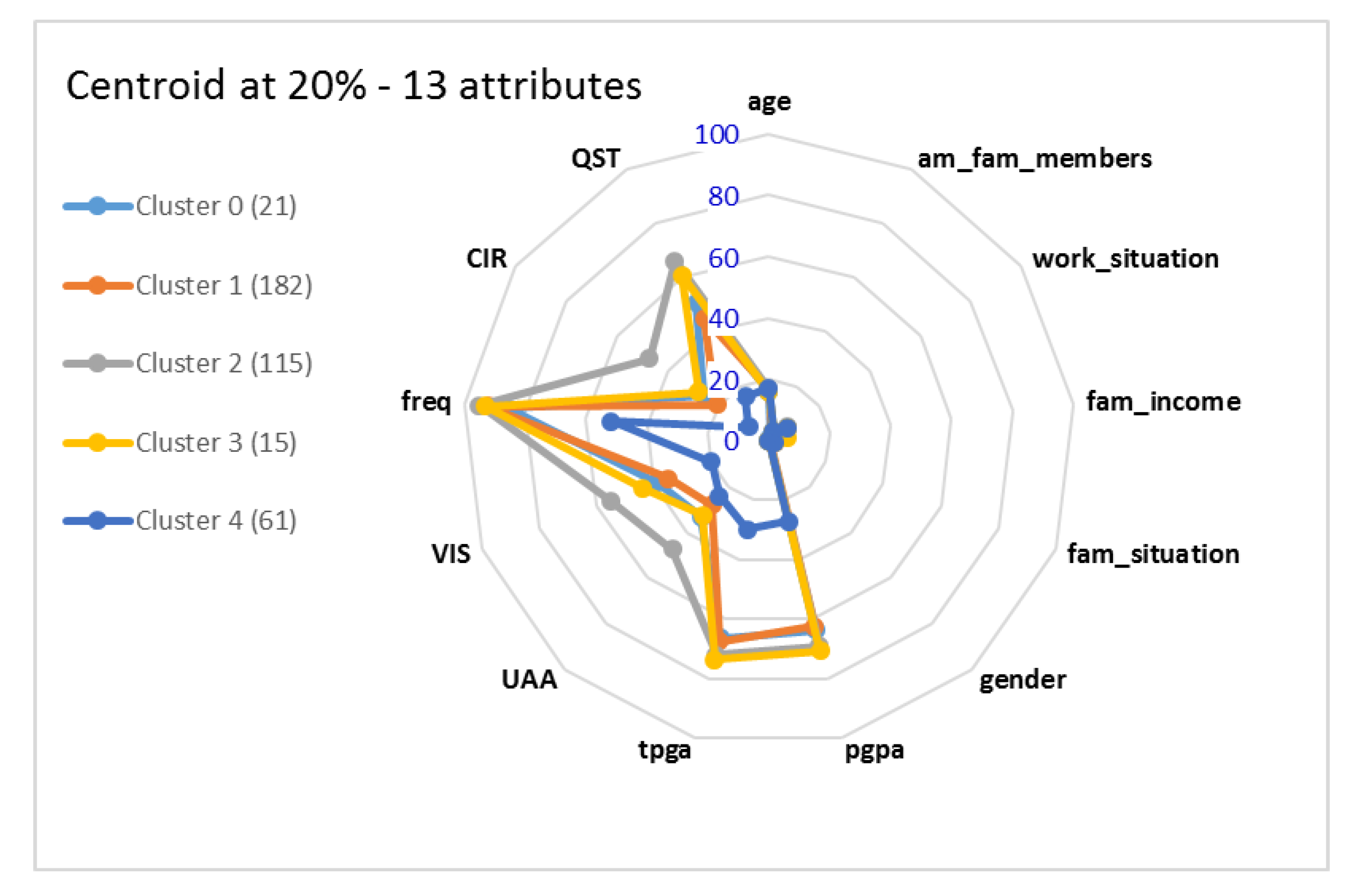
Initially, all attributes were used to find the clusters. The first result, for all data at M1, is shown in Figure 6 as a radar chart representing the coordinates of each cluster. Each polygon in this chart represents one cluster, and each direction is an attribute. This chart gives a sense of which centroids are closer to each other, and may be used to compare the clusters found at different moments.
Figure 6 shows five clusters, numbered arbitrarily from 0 to 4. We can see there are a few attributes where the centroids differ more, and that there are a few attributes that have no impact on the clustering, namely age, gender, am_fam_members, and fam_situation. After this first set of clusters was found, we removed the irrelevant attributes and ran K-means again. This time the attribute work_situation was found to have no impact on the clustering and was removed before we ran the clustering algorithm again. The attribute fam_income, which is missing values for 50.56% of the instances, was also removed. Finally, we ran the K-means algorithm. The last set of clusters at M1 is shown in Figure 7 as a centroid chart.
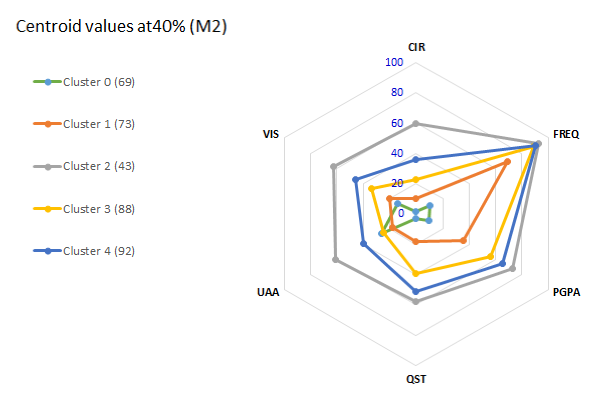
We repeated the same procedure at M2 and M3, starting with all attributes, and then pruning to the same 6 features. At M2 (Figure 8), the 5 clusters have similar characteristics to M1. The number of students differs, however, because between M1 and M2 there is a transition from the 1st. to the 2nd. semester and some students abandon the course.
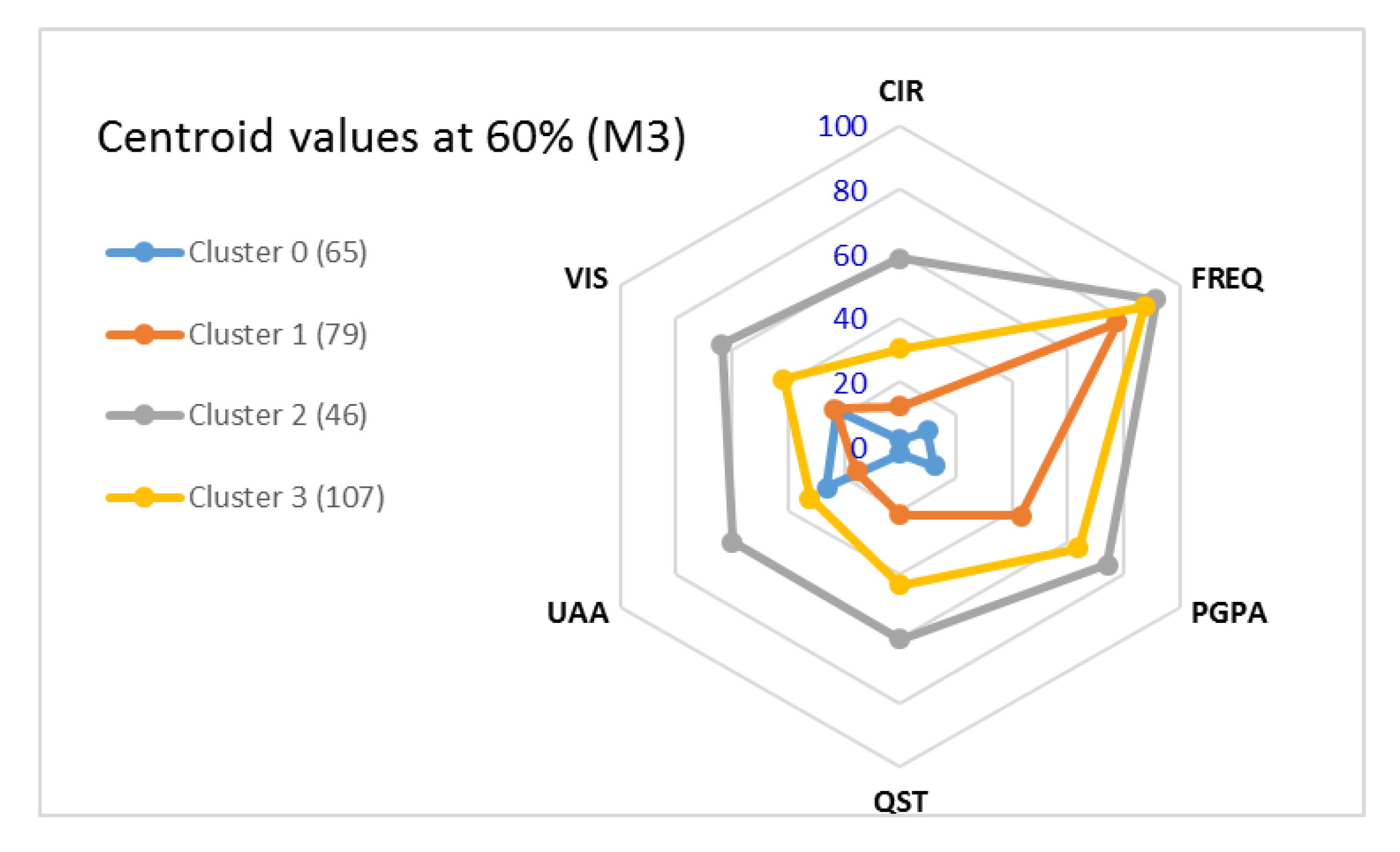
At M3 (Figure 9), we find the best k = 4, which indicates closer distances between the values than those found in M1 and M2. As the course progresses, we are able to identify fewer groups that better define the characteristics of the classes that would later succeed or fail in completing the course.
Now we analyze the data of the clusters. For each attribute per cluster, we extracted its median, mean, lower, and upper quartiles at M1, M2, and M3. This gives insight on the dispersion and central tendency of the data sets. Results are in Table 6.
It is important to remember that each cluster contains students from both the positive and negative classes. Therefore, the classification label is not necessarily related to clusters. However, getting to understand the correlations to get as close as possible is part of this work.
The pGPA is the most relevant attribute to find groups of students, with a minimum of 60 points for approval in the subject. In M1 and M2, we have 5 clusters. In M3, there are 4 clusters, 2 from the positive class (cluster_0 and cluster_1) and 2 from the negative class (cluster_2 and cluster_3).
The next most relevant attribute is QST. This maintains a balanced pattern in M1, M2, and M3, with the median and quartiles better delimited than the others for each cluster. Despite several assessment tools in the LMS, teachers prefer to use the questionnaire, and, as a result, it is an attribute with a high correlation with the grade.
The following attribute that becomes relevant is the CIR, with the percentage, in reference to the maximum in the class, of views of the course and resources provided by the teacher, which has a median that follows an ordered sequence with the upper quartile that does not overlap with the lower quartile of the next cluster. Thus, they are well-delimited values to identify each group.
Students with poor CIR scores procrastinate when it comes to viewing course content and teacher-submitted resources. As a result, they may hand in assignments with little reference to these resources.
Thus, the pGPA together with the CIR, better define the standards to find the groups during the course and that a gGPA lower than 55.5 (lower quartile in M3) or a CIR lower than 23.0 (lower quartile in M3) belong the positive class, the non-completers.
There is a weekly attendance and the rest is online. The FREQ (TD1) attribute, considering the 75% minimum attendance requirement, identifies those who do not reach the minimum. This attribute is typically analyzed in any course of any modality and level, confirming its relevance in online tracking. Cluster_0 is the only one in the 3 moments below 75.0, defining who is reproved for lack but does not define who is reproved by other requirements.
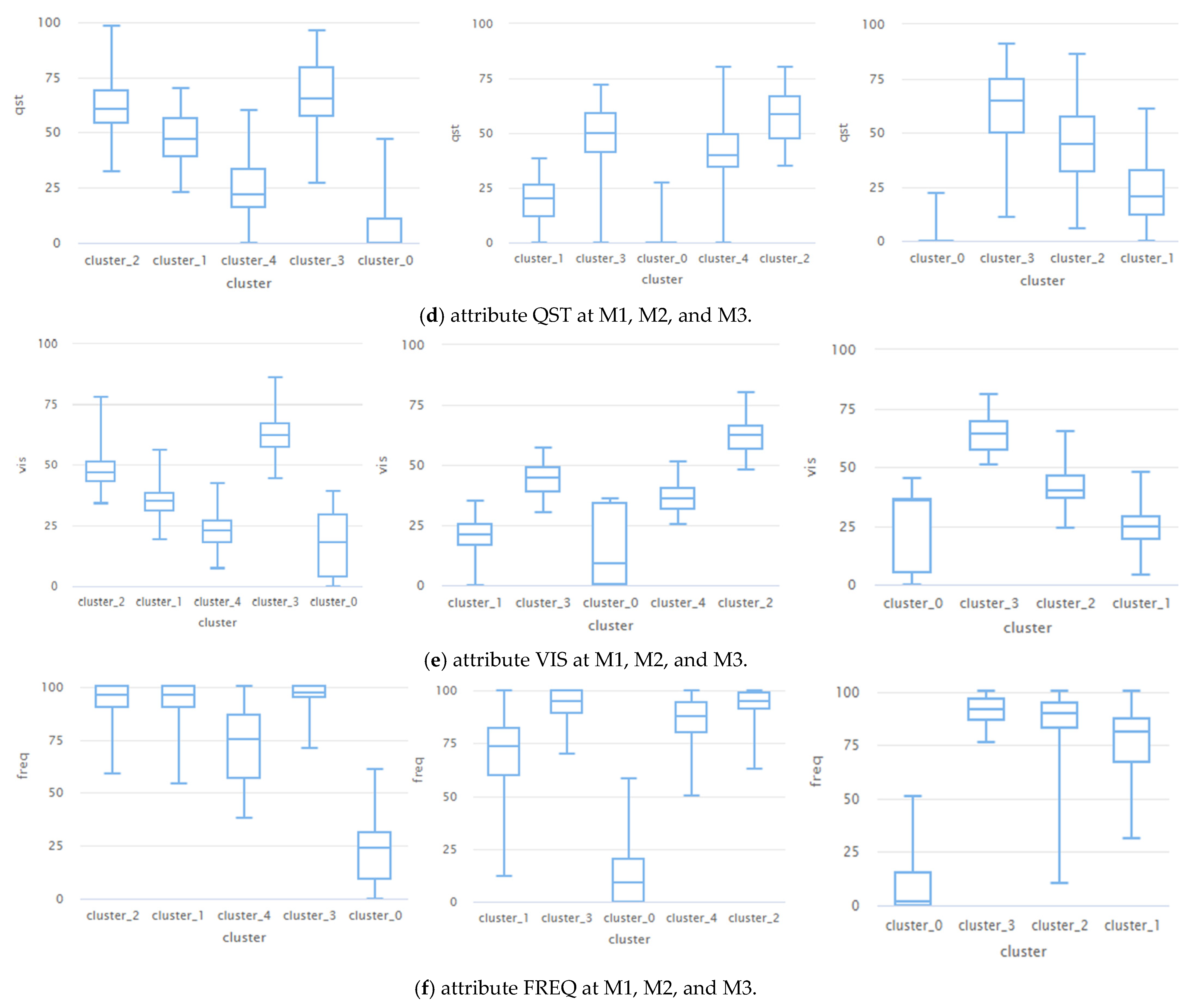
To better visualize the behavior of each of the 6 features that created the clusters, Figure 10 shows, in boxplot form, the median, the mean, the quartiles, their minimum and maximum values of the UAA (TD6), CIR (TD7), pGPA (TD3), QST (TD5), VIS (TD4) and FREQ (TD1). We did the same process in M2 and M3.
In the case of the VIS (TD4) in Figure 10e, they have better-delimited median, minimum and maximum values for each cluster. A deficient VIS value defines a group of students who view significantly less often than the rest. Together with the CIR (Figure 10b), this attribute can identify and discriminate between groups in M1.
To continue with the analysis, we observed that the Cluster_4 at M1 (Figure 7) is very similar to Cluster_1 at M2 (Figure 8) and Cluster_1 at M3 (in Figure 9). We can see the same happens in Figure 10. Although they do not necessarily contain the same instances, they represent the same behavior of students at different moments of analysis. We identified equivalence between clusters at all moments, and this equivalence is reported in Table 7. At this point, we break down the clusters by status, which are “drop-out” (D), “fail” (F), and “passed” (P).
- ◦
- Although the status was not used as part of the clustering (it was the target in our classification problem), most clusters show a distribution of students that reflect their future condition (passed, fail, or drop-out);
- ◦
- Several cases at M1 still do not fit the characteristics of a student who will later drop out or fail. Yet, as one progresses to M2 and M3, we can see that it has a status that stands out by the majority in each cluster;
- ◦
- We have identified a group of students who have never or seldom accessed the LMS, which is Cluster_0 (M1, M2, and M3). As one may see in the boxplots (Figure 10) the centroid has all attributes with a minimum value of 0 or close to 0. For M1, it found 25 students, 10% of class P (status D + F), 71 students at M2, 30% of class P, and 64 students at M3, 36% of the total 175 in class P (Table 7). Performance drops as time passes;
- ◦
- At M1 (Table 7), the first two groups concentrate on those who do not finish, and the last two groups focus on those who complete. In instances from the intermediate cluster (cluster_1 in M1, cluster_4 in M2), concentrate the average values in their attributes (Figure 10). There is a similar amount of classes N and P, not managing to determine a group, but which dissipates in M2 and can better determine in M3, whether it belongs to the first two groups or the last two groups, eliminating the intermediate group;
- ◦
- Class P is mainly concentrated in cluster_0, cluster_4, and cluster_1 in M1 (Table 7), with lower values in all attributes (Figure 9), and cluster_0 (predominant dropout) has minimum values of 0 in all attributes. This value includes cases with no interaction in the LMS, while cluster 1 (predominant failure) always has better values but not enough to complete successfully;
- ◦
- ◦
- In M1, cluster_0 and cluter_4 indicate low performance in all attributes, except for FREQ where cluster_0 is very low, and in cluster_4 it is high, which suggests that cluster_0 corresponds to those who do not attend or reach a passing grade and cluster_4 are those who attend but don’t get enough grade to approve;
- ◦
- The best performance is obtained by students who have high results in the assessment, attendance, visualization of the course, and resources provided by the teacher. Just one of them is not enough;
- ◦
- Of the students who started well (cluster_2 and cluster_3 at M1), 73 cases with D (dropout) and F(failed) status out of the 262 in class P, 28% failed to complete the course. On the other hand, only 2 students with status P (passed) in cluster_0 and cluster_4 at M1 start with difficulties and then improve to complete the course, not even 2% of class N.
The summary of our findings is shown in the last section, and we can now answer RQ3. Initially, we detected five groups of students, valid for forecast moments in M1 (20% of course completion) and M2 (40%), which group the students in terms of their interaction with the LMS. Notably, the single assessment-related variable (pGPA) does not by itself determine group membership.
The K-means algorithm finds, for each prediction moment, behavior patterns that are highly correlated with the performance of students belonging to such groups, with pGPA and CIR being those that better define the clusters. It finds five patterns in M1 and M2 and four patterns in M3.
It is impossible to state that a student cluster at M1 stayed or changed clusters in M2. We would need an analysis per student, but by the total amounts in the clusters, together with the statuses, we can identify the permanence or changes of groups. Further study would be needed to detect individual student behavior changes.
Limitation
This study must be interpreted within the following limitations: (a) the results may be subject to the automated engines of the RapidMiner tool; (b) there may be some bias involved in the resources initially selected to build the dataset from the records and decisions to deal with the missing data.
6. Discussion
This paper presented a supervised model, using classification techniques for predicting students at risk of dropping out, and an unsupervised analysis to gather insight on the behavior of students for a Learning Management System.
We trained classification models to predict students’ performance with data collected from students of nine classes of three courses, all of which are 2-year dual-enrollment technical courses in distance education mode with data at 20% of the course completion (M1), 40% of course completion (M2), and 60% of course completion (M3). Training and test data for Machine Learning algorithms were assembled with features engineered from Moodle log data, as well as socio-economic data provided by the students as of their admittance in the course.
By analyzing the correlation of the attributes with class, we verified that socio-economic data make for poor attributes to identify student performance. This may be partly explained by the fact that a large proportion of the data is missing, such as family income, which students often decline to provide, and employment status. On the other hand, we confirmed that some Moodle data makes for very useful attributes. One example is the low overall score in Moodle activities, which indicates that the student is prone to fail or drop out. Little engagement with Moodle activities is an early warning sign and becomes an important predictor of failure at M2 and M3.
The results suggest that RF (Random Forest) and DT (Decision Tree) are the best models to predict students at risk of dropping out in the course’s first 5–6 subjects (M1). Tree-based models are relatively easy to interpret and thus allow not only to identify at-risk students with high confidence but also to understand the possible reasons for dropout. The NB (Naive Bayes), based on statistical calculations, proved to be efficient from the middle of the course onwards.
Clustering by K-means resulted in 5 behavior patterns in the LMS up to M1 and four more clearly defined patterns when reaching M3, two groups for class N (success) and two groups for class P (fail).
In addition to the mean of the activity grades (pGPA), the most relevant variable was CIR (access to the course and teacher resources), which proved the most pertinent predictor with the target value. This conclusion coincides with the list of the most relevant attributes found in the classification techniques (Table 5), without the tGPA, excluded from K-means. It also coincides with the tree in Figure 4 that shows pGPA and CIR, with values that define classes N and P, and manages to separate 236 of the 262 cases of class P, i.e., 90%.
It is important to remember that students in the classes we analyzed attend regular high school while simultaneously taking a course to obtain the title of technician. Secondary education is a difficult stage for students to prepare for the college preparation exam and the job market, contributing to dropout from the technical course. On the other hand, they are motivated to have this training and diploma, which better prepares them to get a job, prepare for higher education studies, and increase self-esteem.
It is also worthwhile to remark that our studies were carried out with data from classes completed by the end of 2019, therefore before the start of the SARS-CoV-2 pandemic. After that, however, new studies may be carried out, and a similar analysis could be performed to consider the impact of social isolation throughout the course and how the adoption of remote classrooms has affected presential or semi-presential.
7. Conclusions
The contribution of this work is to provide a performance prediction model for students at risk of dropping out using Machine Learning techniques on Moodle-LMS logs of technical courses concomitant with high school, a level of education that is still little explored.
In summary, our findings are as follows:
- The first two groups (Table 7) concentrate on those who do not finish, and the last two groups focus on those who complete. The intermediate cluster does not manage to determine a group, but which dissipates in M2 and can better determine in M3, eliminating the middle group;
- The first cluster (predominant dropout) without interaction in the LMS, while the second cluster (predominant failure) has better values and good class attendance but not enough to complete successfully;
- Approximately 28% of the students who start well fail to complete the course. In comparison, only 2% of those who begin with difficulties in the assessments manage to overcome themselves and complete the course;
- Students with lower assessment scores do not access or view teacher resources.
Finally, the model allows the adoption of measures that contribute to the personalized monitoring of students and the detection of students at risk of dropping out, as it can serve as an instrument for decision-making in school intervention.
Author Contributions
Formal analysis, M.M.T. and R.G.; Investigation, M.M.T.; Methodology, M.M.T. and R.G.; Project administration, M.M.T.; Software, M.M.T. and R.G.; Supervision, R.G.; Validation, R.G.; Visualization, J.F.d.M.N.; Writing—original draft, M.M.T.; Writing—review & editing, R.G. All authors have read and agreed to the published version of the manuscript.
Funding
This research, carried out within the scope of the Samsung-UFAM Project for Education and Research (SUPER), according to Article 48 of Decree nº 6.008/2006(SUFRAMA), was funded by Samsung Electronics of Amazonia Ltda., under the terms of Federal Law nº 8.387/1991, through agreement 003/2019 and 001/2020, signed with Federal University of Amazonas and FAEPI, Brazil.
Institutional Review Board Statement
The study was approved by the Ethics Committee of Federal University of Amazonas, protocol code 88677018.3.0000.5020 date of approval on July 5, 2018, for studies involving humans.
Acknowledgments
We thank the Federal Institute of Education, Science and Technology of Rondonia State (IFRO) for providing the database and administrative support. This work was partially supported by Amazonas State Research Support Foundation—FAPEAM.
Conflicts of Interest
The authors declare no conflict of interest.
References
- Means, B.; Toyama, Y.; Murphy, R.; Bakia, M.; Jones, K. Evaluation of Evidence-Based Practices in Online Learning: A Meta-Analysis and Review of Online Learning Studies; Repository.alt.ac.uk: Washington, DC, USA, 2009. [Google Scholar]
- Marek, M.W.; Chew, C.S. Teacher Experiences in Converting Classes to Distance Learning in the COVID-19 Pandemic. Int. J. Distance Educ. Technol. 2021, 19, 40–60. [Google Scholar] [CrossRef]
- Alturki, U.; Aldraiweesh, A. Application of Learning Management System (LMS) during the COVID-19 Pandemic: A Sustainable Acceptance Model of the Expansion Technology Approach. Sustainability 2021, 13, 10991. [Google Scholar] [CrossRef]
- Mitchell, T. Machine Learning; McGraw-Hill: New York, NY, USA, 1997; p. 432. ISBN 0070428077. [Google Scholar]
- Seidman, A. Retention revisited: R=E, id+E & In, iv. Coll. Univ. 1996, 71, 18–20. [Google Scholar]
- Barnes, T.; Desmarais, M.; Romero, C.; Ventura, S. Educational Data Mining. In Proceedings of the 2nd International Conference Educational Data Mining, Cordoba, Spain, 1–3 July 2009. [Google Scholar]
- Zamfiroiu, A.; Constantinescu, D.; Zurini, M.; Toma, C. Secure Learning Management System Based on User Behavior. Appl. Sci. 2020, 10, 7730. [Google Scholar] [CrossRef]
- Balkaya, S. Role of Trust, Privacy Concerns and Data Governance in Managers’ Decision on Adoption of Big Data Systems. Manag. Stud. 2019, 7, 229–237. [Google Scholar] [CrossRef] [Green Version]
- Balkaya, S.; Akkucuk, U. Adoption and Use of Learning Management Systems in Education: The Role of Playfulness and Self-Management. Sustainability 2021, 13, 1127. [Google Scholar] [CrossRef]
- Kotsiantis, S.; Pierrakeas, C.; Pintelas, P. Predicting students’ performance in distance learning using machine learning techniques. Appl. Artif. Intell. 2004, 15, 411–426. [Google Scholar] [CrossRef]
- Lee, S.; Choi, Y.-J.; Kim, H.-S. The Accurate Measurement of Students’ Learning in E-Learning Environments. Appl. Sci. 2021, 11, 9946. [Google Scholar] [CrossRef]
- Anil, K.J. Data Clustering: 50 Years beyond K-Means, Pattern Recognition Letters; Elsevier: Amsterdam, The Netherlands, 2010; Volume 31, pp. 651–666. ISSN 0167-8655. [Google Scholar] [CrossRef]
- Tamada, M.M.; Netto, J.F.M.; Lima, D.P.R. Predicting and Reducing Dropout in Virtual Learning using Machine Learning Techniques: A Systematic Review. In Proceedings of the 2019 IEEE Frontiers in Education Conference (FIE), Covington, KY, USA, 16–19 October 2019. [Google Scholar] [CrossRef]
- Andrade, T.L.; Rigo, S.J.; Barbosa, J.L. Active Methodology, Educational Data Mining and Learning Analytics: A Systematic Mapping Study. Inform. Educ. 2021, 20, 171–204. [Google Scholar] [CrossRef]
- Karlos, S.; Aridas, C.; Kanas, V.G.; Kotsiantis, S. Classification of acoustical signals by combining active learning strategies with semi-supervised learning schemes. Neural Comput. Appl. 2021. [Google Scholar] [CrossRef]
- Ljubobratović, D.; Matetić, M. Using LMS activity logs to predict student failure with random forest algorithms. In Proceedings of the Future of Information Sciences, Zagreb, Croatia, 21–22 November 2019; p. 113. [Google Scholar] [CrossRef]
- Burgos, C.; Campanario, M.L.D.; Peña, D.L.; Lara, J.A.; Lizcano, D.; Martínez, M.A. Data mining for modeling students performance: A tutoring action plan to prevent academic dropout. Comput. Electr. Eng. 2018, 66, 542–556. [Google Scholar] [CrossRef]
- Isidro, C.; Carro, R.M.; Ortigosa, A. Dropout detection in MOOCs: An exploratory analysis. In Proceedings of the 2018 International Symposium on Computers in Education (SIIE), Cadiz, Spain, 19–21 September 2018; pp. 1–6. [Google Scholar] [CrossRef]
- Xing, W.; Du, D. Dropout Prediction in MOOCs: Using Deep Learning for Personalized Intervention. J. Educ. Comput. Res. 2019, 57, 547–570. [Google Scholar] [CrossRef]
- Conijn, R.; Snijders, C.; Kleingeld, A.; Matzat, U. Predicting student performance from LMS data: A comparison of 17 blended courses using Moodle LMS. IEEE Trans. Learn. Technol. 2017, 10, 17–29. [Google Scholar] [CrossRef]
- López-Zambrano, J.; Lara, J.A.; Romero, C. Towards portability of models for predicting students’ final performance in university courses starting from Moodle logs. Appl. Sci. 2020, 10, 354. [Google Scholar] [CrossRef] [Green Version]
- Hung, J.-L.; Zhang, K. Revealing online learning behaviors and activity patterns and making predictions with data mining techniques in online teaching. MERLOT J. Online Learn. Teach. 2008, 4, 426–437. [Google Scholar]
- Talavera, L.; Gaudioso, E. Mining student data to characterize similar behavior groups in unstructured collaboration spaces. In Proceedings of the Workshop on Artificial Intelligence in CSCL, 16th European Conference on Artificial intelligence, Valencia, Spain, 22–27 August 2004; pp. 17–23. [Google Scholar]
- Cerezo, R.; Sanchez-Santillan, M.; Paule-Ruiz, M.P.; Núñez, J.C. Students’ LMS interaction patterns and their relationship with achievement: A case study in higher education. Comput. Educ. 2016, 96, 42–54. [Google Scholar] [CrossRef]
- Romero, C.; López, M.-I.; Luna, J.-M.; Ventura, S. Predicting students’ final performance from participation in on-line discussion forums. Comput. Educ. 2013, 68, 458–472. [Google Scholar] [CrossRef]
- Riestra-González, M.; Paule-Ruíz, M.D.P.; Ortin, F. Massive LMS log data analysis for the early prediction of course-agnostic student performance. Comput. Educ. 2021, 163, 104108. [Google Scholar] [CrossRef]
- Neto, F.A.; Castro, A. Elicited and mined rules for dropout prevention in online courses. In Proceedings of the 2015 IEEE Frontiers in Education Conference, El Paso, TX, USA, 21–24 October 2015; Volume 1, pp. 1–7. [Google Scholar] [CrossRef]
- RapidMiner, Lightning Fast Data Science Platform for Teams. Available online: https://rapidminer.com (accessed on 22 July 2020).
- Powers, D.M.W. Evaluation: From precision, recall and F-measure to ROC, informedness, markedness & correlation. J. Mach. Learn. Technol. 2011, 2, 37–63. [Google Scholar] [CrossRef]
- Derczynski, L. Complementarity, F-score, and NLP Evaluation. In Proceedings of the International Conference Language Resource Evaluation, (LREC’16), Portorož, Slovenia, 23–28 May 2016; pp. 261–266. [Google Scholar]
- Hastie, T.; Tibshirani, R.; Friedman, J. The Elements of Statistical Learning: Data Mining, Inference, and Prediction, 2nd ed.; Springer: Cham, Switzerland, 2008; ISBN 978-0-387-84858-7. [Google Scholar]
- Piryonesi, S.M.; El-Diraby, T.E. Using Machine Learning to Examine Impact of Type of Performance Indicator on Flexible Pavement Deterioration Modeling. J. Infrastruct. Syst. 2021, 27, 04021005. [Google Scholar] [CrossRef]
- Han, J.; Pei, J.; Kamber, M. Data Mining: Concepts and Techniques; Elsevier: Amsterdam, The Netherlands, 2011; p. 744. [Google Scholar]
Figure 1.
Model preparation and construction.

Figure 2.
Classification algorithms metrics: (a) Precision metric; (b) Recall metric.

Figure 3.
Performance of the F1 metric of each algorithm at each point in time M1, M2, M3.

Figure 4.
Confusion matrices for the SVM classifier.

Figure 5.
Classification Decision Tree at M1: (a) pgpa <= 60.5; (b) pgpa between (60.5, 85.5) and cir <= 12; (c) pgpa between (60.5, 85.5) and cir > 12.
Figure 5.
Classification Decision Tree at M1: (a) pgpa <= 60.5; (b) pgpa between (60.5, 85.5) and cir <= 12; (c) pgpa between (60.5, 85.5) and cir > 12.

Figure 6.
K-means summary at M1. Polygons are cluster centroids and points represent the value of the centroid for each attribute.
Figure 6.
K-means summary at M1. Polygons are cluster centroids and points represent the value of the centroid for each attribute.

Figure 7.
Clustering at M1.

Figure 8.
Clustering at M2.

Figure 9.
Clustering at M3.

Figure 10.
Boxplot by clusters in M1, M2 and M3 for each attribute; (a) UAA; (b) CIR; (c) pGPA; (d) QST; (e) VIS; (f) FREQ.
Figure 10.
Boxplot by clusters in M1, M2 and M3 for each attribute; (a) UAA; (b) CIR; (c) pGPA; (d) QST; (e) VIS; (f) FREQ.


Table 1.
Summary of the literature review of distance learning students’ performance prediction.
| Ref | Approach | Year | Algorithms | Target | Overview |
|---|---|---|---|---|---|
| [16] | Classification | 2019 | Random Forest | final grade | Laboratory and questionnaire scores have the most significant influence on the final grade. |
| [17] | Classification | 2017 | Logistic Regression | dropout | A tutoring action plan that presented a 14% reduction in the dropout rates. |
| [18] | Classification | 2018 | Deep Learning | dropout | Models based on a weekly analysis. They generated 42 predictive models, one for each week. |
| [19] | Classification | 2018 | Deep Learning | dropout | Prediction model using data from the past few weeks to predict whether a student will drop out in the following week. |
| [20] | Regression | 2017 | Logistic Regression | final grade | Using logistic (pass/fail) and standard regression (final grade) models for 10 weeks. |
| [26] | Classification | 2021 | Multilayer Perceptron | solving tasks | Models for the initial prediction of student performance in solving tasks in LMS, just analyzing the Moodle log files generated up to the time of prediction. |
| [23] | Cluster analysis | 2004 | Expectation-Maximization | N/A | Found six clusters with LMS interaction patterns from one course. |
| [22] | Cluster analysis | 2008 | K-means | N/A | Finding three clusters with patterns of learning behavior using surveys. |
| [25] | Cluster analysis | 2013 | Expectation-Maximization | final marks | Use of different data mining approaches for improving prediction of students’ final performance using forum data. |
| [24] | Cluster plus association analysis | 2016 | K-means; Expectation-Maximization | N/A | Found four clusters studying students’ asynchronous learning process. |
| [26] | Cluster analysis | 2021 | K-means | solving tasks | Creating course-agnostic clusters generalizing 699 courses in different areas, types, and periods at 10%, 25%, 33%, and 50% of the course duration |
Table 2.
Distribution of classes for each course and moments. Rows are related to the three courses and columns refer to the moment of collection (at 20%, 40%, and 60% of course completion). The positive class (P) refers to students who did not graduate after three years and the negative class (N) refers to students who did graduate.
| M1 (20%) | M2 (40%) | M3 (60%) | ||||
|---|---|---|---|---|---|---|
| N | P | N | P | N | P | |
| IPI (Informatics) | 34 | 98 | 34 | 96 | 34 | 64 |
| ADM (Administration) | 68 | 108 | 64 | 87 | 59 | 64 |
| FIN (Finance) | 30 | 56 | 29 | 55 | 29 | 47 |
| Total | 132 | 262 | 127 | 238 | 122 | 175 |
| % | 33.5 | 66.5 | 34.79 | 65.21 | 41.08 | 58.92 |
| Total enrolled | 394 | 365 | 297 | |||
Table 3.
Institutional Data Attributes. These data are collected from students at admission.
| Institutional Data (ID) | ||||
|---|---|---|---|---|
| Code | Name | Type | Description | Values |
| ID1 | age | continuous | variable calculated | 14 to 19 years old |
| ID2 | gender | categorical | ||
| ID3 | fam_income | continuous | family income in number of minimum wages | |
| ID4 | am_fam_members | continuous | number of people in the family | |
| ID5 | work_situation | categorical | family work situation | 1-Unemployed, 2-Professional, 3-Employed, 4-Retired, 5-Entrepreneur, 6-Self-employed, 7-Cooperated |
| ID6 | fam_situation | categorical | income share | 1—Income Provider; 2—Dependent; 3—Make up the income |
| ID7 | status | categorical | final status | “passed”, “completed”, “apt to graduate”, “dropout”, “failed”, “abandon” |
Table 4.
Traced Data Attributes, collected from Moodle data. They are aggregated according to their description and normalized to the 0–100 interval.
Table 4.
Traced Data Attributes, collected from Moodle data. They are aggregated according to their description and normalized to the 0–100 interval.
| Trace Data (TD) | ||||
|---|---|---|---|---|
| Code | Name | Type | Description | Values |
| TD1 | FREQ | continuous | student attendance | 0–100 |
| TD2 | tGPA | continuous | Total GPA with an average of the final grades of the subjects by the defined forecast time in the duration of the course. | 0–100 |
| TD3 | pGPA | continuous | Progress GPA with average of submitted activities grades. 2 courses activities per subject are required | 0–100 |
| TD4 | VIS | continuous | percentage of visualization of modules, tasks, forums, quizzes, etc. | 0–100 |
| TD5 | QST | continuous | percentage of viewing, accessing, answering attempts, and answering questionnaires | 0–100 |
| TD6 | UAA | continuous | percentage of access to external materials and submitted tasks | 0–100 |
| TD7 | CIR | continuous | percentage of access to course and resources | 0–100 |
Table 5.
Weights of attributes according to Pearson correlation: (a) at M1 (20%); (b) at M2 (40%); (c) at M3 (60%).
Table 5.
Weights of attributes according to Pearson correlation: (a) at M1 (20%); (b) at M2 (40%); (c) at M3 (60%).
| M1 (20%) | M2 (40%) | M3 (60%) | |||
|---|---|---|---|---|---|
| Attribute | Weight | Attribute | Weight | Attribute | Weight |
| pGPA | 0.494 | pGPA | 0.642 | pGPA | 0.662 |
| tGPA | 0.446 | tGPA | 0.610 | tGPA | 0.630 |
| QST | 0.379 | CIR | 0.559 | CIR | 0.591 |
| VIS | 0.366 | VIS | 0.527 | QST | 0.557 |
| CIR | 0.359 | QST | 0.503 | VIS | 0.554 |
| freq | 0.332 | freq | 0.494 | freq | 0.535 |
| UAA | 0.265 | UAA | 0.451 | UAA | 0.444 |
| age | 0.186 | age | 0.186 | age | 0.187 |
| gender | 0.097 | gender | 0.106 | fam_income | 0.087 |
| fam_income | 0.088 | fam_income | 0.084 | gender | 0.083 |
| am_fam_members | 0.041 | am_fam_members | 0.032 | am_fam_members | 0.007 |
Table 6.
Median, lower quartile, the upper quartile of clusters by attributes at M1, M2, M3.
| UAA | CIR | pGPA | QST | VIS | FREQ | ||||||||||||||
|---|---|---|---|---|---|---|---|---|---|---|---|---|---|---|---|---|---|---|---|
| Median | Lower | Upper | Median | Lower | Upper | Median | Lower | Upper | Median | Lower | Upper | Median | Lower | Upper | Median | Lower | Upper | ||
| M1 | cluster_0 | 33.44 | 26.00 | 33.44 | 0.60 | 0.00 | 4.20 | 13.00 | 0.00 | 32.50 | 0.20 | 0.00 | 10.50 | 18.00 | 3.88 | 29.00 | 24.00 | 9.00 | 31.00 |
| cluster_4 | 17.75 | 12.00 | 27.75 | 9.00 | 6.00 | 15.00 | 38.00 | 31.25 | 49.00 | 22.00 | 15.70 | 33.00 | 23.00 | 18.00 | 27.00 | 75.50 | 57.00 | 86.75 | |
| cluster_1 | 28.00 | 20.40 | 33.33 | 18.00 | 14.00 | 25.00 | 63.00 | 54.00 | 70.00 | 47.00 | 39.00 | 56.00 | 35.00 | 31.00 | 38.00 | 96.00 | 90.00 | 100.00 | |
| cluster_2 | 37.00 | 32.00 | 43.70 | 34.00 | 29.00 | 43.85 | 70.00 | 63.00 | 77.75 | 60.80 | 54.00 | 69.00 | 47.00 | 43.00 | 51.00 | 96.00 | 90.25 | 100.00 | |
| cluster_3 | 58.50 | 45.60 | 68.90 | 60.50 | 47.00 | 67.25 | 73.50 | 64.50 | 79.00 | 65.60 | 57.50 | 79.00 | 62.00 | 57.15 | 67.00 | 97.50 | 94.75 | 100.00 | |
| M2 | cluster_0 | 31.72 | 22.00 | 31.72 | 0.00 | 0.00 | 1.00 | 0.00 | 0.00 | 11.00 | 0.00 | 0.00 | 0.00 | 9.17 | 0.33 | 33.76 | 9.00 | 0.00 | 20.00 |
| cluster_1 | 16.00 | 10.15 | 26.25 | 9.00 | 6.00 | 13.25 | 37.50 | 27.00 | 47.00 | 20.00 | 12.00 | 26.08 | 21.00 | 16.75 | 25.00 | 73.50 | 59.75 | 82.25 | |
| cluster_4 | 25.30 | 18.13 | 32.50 | 23.25 | 18.83 | 31.00 | 51.00 | 43.00 | 60.25 | 40.00 | 34.28 | 49.25 | 35.91 | 31.50 | 40.00 | 95.00 | 91.00 | 100.00 | |
| cluster_3 | 38.67 | 32.00 | 45.00 | 34.00 | 25.00 | 41.00 | 71.00 | 63.00 | 79.00 | 50.00 | 41.00 | 59.04 | 44.67 | 38.75 | 49.00 | 95.00 | 89.00 | 100.00 | |
| cluster_2 | 31.50 | 54.00 | 67.00 | 56.50 | 48.00 | 69.96 | 70.50 | 67.00 | 81.75 | 58.42 | 47.25 | 66.75 | 62.41 | 56.25 | 66.13 | 88.00 | 80.00 | 94.25 | |
| M3 | cluster_0 | 30.71 | 30.71 | 30.71 | 0.00 | 0.00 | 2.00 | 0.00 | 0.00 | 21.25 | 0.00 | 0.00 | 0.00 | 35.93 | 5.04 | 35.93 | 2.00 | 0.00 | 15.00 |
| cluster_1 | 14.00 | 9.00 | 21.00 | 11.50 | 5.96 | 18.38 | 43.00 | 34.00 | 53.00 | 20.50 | 11.75 | 32.25 | 24.50 | 19.00 | 28.75 | 81.00 | 67.00 | 87.00 | |
| cluster_2 | 32.00 | 24.83 | 39.50 | 30.00 | 23.00 | 37.50 | 63.00 | 55.50 | 74.50 | 44.50 | 32.00 | 57.00 | 40.00 | 36.83 | 45.91 | 90.00 | 83.00 | 95.00 | |
| cluster_3 | 59.33 | 49.00 | 70.25 | 58.00 | 48.79 | 65.25 | 74.00 | 68.00 | 81.00 | 64.50 | 50.00 | 74.25 | 64.00 | 56.88 | 69.00 | 92.00 | 86.75 | 96.25 | |
Table 7.
Clusters and instances by status.
| M1 (20%). | M2 (40%) | M3 (60%) | |||||||||
|---|---|---|---|---|---|---|---|---|---|---|---|
| cluster_0 | D | 21 | cluster_0 | D | 70 | cluster_0 | D | 56 | |||
| cluster_0 | F | 4 | 25 | cluster_0 | F | 1 | 71 | cluster_0 | F | 8 | 64 |
| cluster_4 | P | 2 | cluster_1 | P | 4 | cluster_1 | P | 9 | |||
| cluster_4 | D | 47 | cluster_1 | D | 29 | cluster_1 | D | 5 | |||
| cluster_4 | F | 7 | 56 | cluster_1 | F | 41 | 74 | cluster_1 | F | 68 | 82 |
| cluster_1 | P | 33 | cluster_4 | P | 14 | ||||||
| cluster_1 | D | 36 | cluster_4 | D | 14 | ||||||
| cluster_1 | F | 74 | 143 | cluster_4 | F | 58 | 86 | ||||
| cluster_2 | P | 67 | cluster_3 | P | 72 | cluster_2 | P | 73 | |||
| cluster_2 | D | 34 | cluster_3 | D | 9 | cluster_2 | D | 5 | |||
| cluster_2 | F | 23 | 124 | cluster_3 | F | 9 | 90 | cluster_2 | F | 27 | 105 |
| cluster_3 | P | 30 | cluster_2 | P | 37 | cluster_3 | P | 40 | |||
| cluster_3 | D | 7 | cluster_2 | D | 2 | ||||||
| cluster_3 | F | 9 | 46 | cluster_2 | F | 5 | 44 | cluster_3 | F | 6 | 46 |
| Students | 394 | Students | 365 | Students | 297 | ||||||
Publisher’s Note: MDPI stays neutral with regard to jurisdictional claims in published maps and institutional affiliations. |
© 2022 by the authors. Licensee MDPI, Basel, Switzerland. This article is an open access article distributed under the terms and conditions of the Creative Commons Attribution (CC BY) license (https://creativecommons.org/licenses/by/4.0/).
Share and Cite
MDPI and ACS Style
Tamada, M.M.; Giusti, R.; Netto, J.F.d.M. Predicting Students at Risk of Dropout in Technical Course Using LMS Logs. Electronics 2022, 11, 468. https://doi.org/10.3390/electronics11030468
AMA Style
Tamada MM, Giusti R, Netto JFdM. Predicting Students at Risk of Dropout in Technical Course Using LMS Logs. Electronics. 2022; 11(3):468. https://doi.org/10.3390/electronics11030468
Chicago/Turabian StyleTamada, Mariela Mizota, Rafael Giusti, and José Francisco de Magalhães Netto. 2022. "Predicting Students at Risk of Dropout in Technical Course Using LMS Logs" Electronics 11, no. 3: 468. https://doi.org/10.3390/electronics11030468
Note that from the first issue of 2016, this journal uses article numbers instead of page numbers. See further details here.