Model Predictive Control-Based Integrated Path Tracking and Velocity Control for Autonomous Vehicle with Four-Wheel Independent Steering and Driving

Abstract

This paper presents an MPC-based integrated control algorithm for an autonomous vehicle equipped with four-wheel independent steering and driving systems. The objective of this research is to improve the performance of the path and velocity tracking controllers by distributing the control effort to the multiple actuators. The proposed algorithm has two modules: reference state decision and MPC-based vehicle motion controller. Reference state decision module determines reference state profiles consisting of yaw rate and velocity in order to overcome the limitation of the error dynamics-based path tracking controller, which requires several assumptions on the reference path. The MPC-based vehicle motion controller is designed with a linear time-varying vehicle model in order to optimally allocate the control effort to each actuator. A linear time-varying MPC is adopted to reduce computational burden caused by using a non-linear one. The effectiveness of the proposed algorithm is validated via simulation on MATLAB/Simulink and CarSim. The simulation results show that the proposed algorithm improves the reference tracking performance by effectively distributing the control effort to the steering angle and driving force of each actuator.

1. Introduction

For the last decade, autonomous driving has attracted intensive attention as a solution needed to improve road safety, traffic efficiency, and the convenience of traffic participants. Various methodologies have been adopted to extend the coverage of application environments and target vehicles in the area of autonomous driving [1,2]. At the beginning of autonomous driving, the operational design domain (ODD) of the autonomous vehicles was restricted to some specific and simple driving environments, such as motorways or parking lots. Thanks to continuous research and developments, the advantages of autonomous driving led to the expansion of application environments, and ODD has been extended beyond urban roads to unconstructed environments [3]. These advances in autonomous driving have been achieved by utilizing the increased number of sensors, processors, actuators, and various information sources, such as vehicle-to-vehicle (V2V) or vehicle-to-infrastructure (V2I) communications. In particular, a larger number of actuators for autonomous vehicles leads to the control allocation problem, which is used to improve the vehicle control performance by coordinating the multiple actuators [4,5,6,7,8]. Since current autonomous vehicles are actuated by the steering, throttle, and brake, researchers have not focused on the problem of motion control. Recently, over-actuated vehicles, such as a purpose-built vehicle (PBV) equipped with in-wheel motors (IWMs) and four-wheel independent steering (4WIS) modules, have been introduced as a platform for future autonomous driving [5,6,7,8]. In order to effectively control the over-actuated vehicles, several research projects have been conducted with the perspective of not only chassis control but also autonomous driving.

Basically, an integrated vehicle control for over-actuated vehicles means the control allocation among various active actuators, which have been introduced to improve the maneuverability of the vehicle or to implement the autonomous driving functions [9,10]. In the area of vehicle chassis control, several actuators have been adopted to improve maneuverability or lateral stability [11,12]. For example, electronic stability control (ESC) with differential braking, torque vectoring devices, electronic-limited slip differential (e-LSD), active suspension, and rear-wheel steering (RWS) have been adopted as an actuator for vehicle chassis control [11,12,13,14]. Recently, E-corner module, which consists of an IWM, brake-by-wire, steer-by-wire, and active suspension has been proposed as a next-generation modular platform for electric and eco-friendly vehicles [9]. For autonomous driving, actuators that can replace the driver’s driving behavior were used to actuate the vehicle. Electric power steering (EPS), throttle-by-wire (TBW), and ESC have been adopted to convert conventional vehicles to autonomous ones [15,16]. Recently, four-wheel independent steering, driving, and braking (4WIS, 4WID, and 4WIB), have been adopted as an actuator for various autonomous vehicles such as passenger cars, autonomous shuttles or PBV [5,9].

The key function in autonomous driving is path and velocity tracking controls which try to make a vehicle follow given path and velocity profiles, respectively. Various path tracking algorithms for a front wheel steering (FWS) vehicle have been proposed to implement autonomous driving into real vehicles [17]. For path tracking, it is necessary to determine a steering angle of the front wheel. For the purpose, the pure pursuit and the Stanley methods based on geometric relationship between a reference path and a vehicle have been adopted as a path tracking algorithm [17]. To improve path tracking performance, a look-ahead distance in the pure pursuit method was designed as a second-order polynomial considering the braking characteristics of the vehicle [18]. In addition, a receding horizon control was applied to the pure pursuit method in order to improve the path tracking performance under high-speed driving conditions [19]. On the other hand, the parameter optimization based on the particle swarm optimization was introduced to Stanley controller [20]. LQR controller was proposed for the lateral controller using the weight matrices optimization mechanism needed to automatically determine the control gain [21]. To handle the non-linearity of a vehicle, a Takagi–Sugeno (T–S) fuzzy model for output feedback control was proposed [22]. Model predictive control (MPC) based on the Ackerman steered vehicle and non-linear tire model were proposed to balance the performance and computational burden [23,24]. Moreover, a multi-layered MPC was developed to compensate for the modeling error by using three different models [25]. Recently, a learning-based steering control algorithm were proposed to achieve acceptable performance without modeling [26,27,28]. For velocity tracking control, MPC with V2V communication was adopted to reduce the rear-end collision [29]. In addition, optimization-based and learning-based approaches were also introduced to design velocity tracking controllers [30,31].

By virtue of the four-wheel steering and driving (4WS/4WD) system, the potential of chassis control and autonomous driving can be extended. Several algorithms have been proposed to enhance the vehicle stability and maneuverability from the perspective of chassis control [11,32]. Similar to the approaches proposed to enhance the vehicle stability, RWS was adopted to improve the lane-keeping assistant system [33,34,35]. The application scope of 4WS was extended toward the path tracking control of the autonomous vehicle. PI and state feedback controllers based on the path tracking errors were used to calculate the front- and rear-wheel steering angles [36,37]. In addition, LQR and H∞ controllers were adopted to determine the optimal state feedback gain [5,6,38]. Adaptive control was also utilized to compensate for the parametric complexity of the 4WS system, which has more parameter than the FWS vehicle [39,40]. An adaptive MPC scheme was developed based on an autoregressive with exogeneous input model to improve the yaw-motion stability [41]. Moreover, torque distribution to four in-wheel motors was proposed by using hybrid structure considering an adaptive maximum torque search and robust sliding mode control to regulate acceleration slip [42].

Since the 4WS/4WD system is inherently non-linear, various sliding mode control (SMC)-based algorithms have been proposed to consider the non-linearity when determining the control input. By assigning two control points at the front and rear wheels of a vehicle, SMC can be applied to the front- and rear-wheel steering, respectively [7]. Similarly, a parallel steering maneuver, which actuates the front and rear wheels at the same angle, was introduced to simplify the SMC algorithm [43]. Furthermore, several types of SMC algorithms were also used to allocate the control effort to the differential steering system by using integral SMC [8], adaptive multivariable super-twisting control [44], and non-linear gain adjustment [45]. The integrated SMC controller for steering and driving/braking was designed to compensate the external yaw moment needed to improve the path tracking performance [4]. In addition, a robust SMC with a T–S fuzzy model was designed to consider the non-linearity of the vehicle model [46].

MPC-based algorithms have been proposed to design the path and velocity tracking controllers for a vehicle with 4WS/4WD system. A time-invariant linear vehicle model assuming a small steering angle and constant velocity was utilized to design an MPC-based path tracking controller [47]. However, it is difficult for this simple model to maintain performance when the curvature or acceleration increases. To prevent the deviation from the linear section of tire force, an MPC with slip angle constraints has been proposed [48]. In addition, a multi-model based MPC was proposed to improve the performance in various driving conditions [49].

Recently, studies have been proposed to integrate several methods or introduce other methods such as machine learning. An integrated approach of MPC and SMC was developed to follow the path and desired speed simultaneously. In this approach, MPC distributed the yaw moment and SMC calculated the longitudinal forces [50]. Decoupling motion tracker for 4WD was designed based on the inverse model learned by the neural network [51]. This method corrected the reference path to improve the yaw tracking and lateral tacking. Furthermore, a game theory-based controller was proposed to search the Nash equilibrium points between two player models [52].

To reduce the computational burden and complexity of the MPC, MPC itself and a control allocation method were separated [9,10]. In this approach, MPC was used only to determine the desired motion needed to track a reference path, and a control allocation method was used to distribute control efforts into each actuator in order to follow the desired motion. The integrated approach with the maneuver decision and the path planner for the lane changes and intersection crossing scenario was proposed based on the MPC. However, a proper prediction algorithm for surrounding vehicles was not proposed [53]. In addition, the controllers that reflect the operational constraints have been proposed [54]. A method for unmanned aerial vehicles to avoid obstacles has been proposed using an explicit reference governor. This governor combines a dynamic safety margin from obstacles and attraction field toward target position in order to create an auxiliary reference for position controller [54].

From a careful review on the previous studies, the various control algorithms for autonomous vehicles with 4WS/4WD have been proposed to enhance the reference tracking performance. In this paper, the reference tracking means both of path and velocity tracking. Since the path tracking control can be considered as an error feedback regulator, the error dynamics based on the lateral and heading error with respect to the reference path were frequently adopted when defining the MPC problem. This approach required the assumptions on the reference path in order to derive the derivatives of the lateral and heading error, which restricts the road conditions where performance can be achieved. In addition, the 4WIS was frequently regarded as a 4WS system, so control inputs were the front and rear steering angles, which were equally applied to the left and right-side wheels [4,5,6,8,36,38,39,40,41,42,43,44,45]. Furthermore, the effect of the four-wheel independently driving (4WID) on the yaw motion of the vehicle was not considered when designing the path tracking controller.

Based on the literature survey on the previous studies, this paper presents the integrated control algorithm with the path and velocity tracking controllers for autonomous vehicles equipped with 4WIS/4WID. Figure 1 shows the schematic diagram of the proposed algorithm. As shown in Figure 1, the proposed algorithm is composed of two modules: a reference state decision and an MPC-based motion controller. The reference state decision module is introduced to determine the reference yaw rate and velocity, which replace the lateral and heading errors. Then, the MPC-based motion controller directly determines the eight control inputs consisting of four steering angles and four traction forces generated by 4WIS/4WID in order to track the reference states. To validate the performance of the proposed algorithm, simulation was conducted via co-simulation on MATLAB/Simulink and CarSim.

The key contributions in this work are summarized as follows:

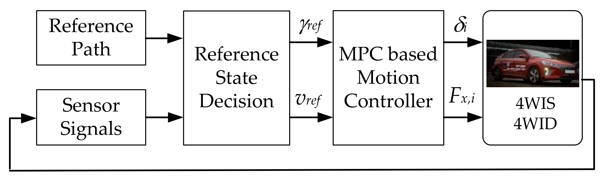
• In the proposed algorithm, the path tracking and velocity controllers determine the control inputs, required for autonomous vehicles with 4WIS/4WID, with a single integrated controller, which distributes the control efforts into the steering angle and wheel torque of each wheel.
• The reference states can be determined without assumptions on the road shapes and vehicle models. Therefore, the reference state decision module can be used for various road conditions and vehicle systems.
• The proposed MPC controller uses the vehicle model as a constraint. The vehicle model is not included in other modules. Therefore, even if the actuator configuration changes, it can only be used by modifying the constraint.

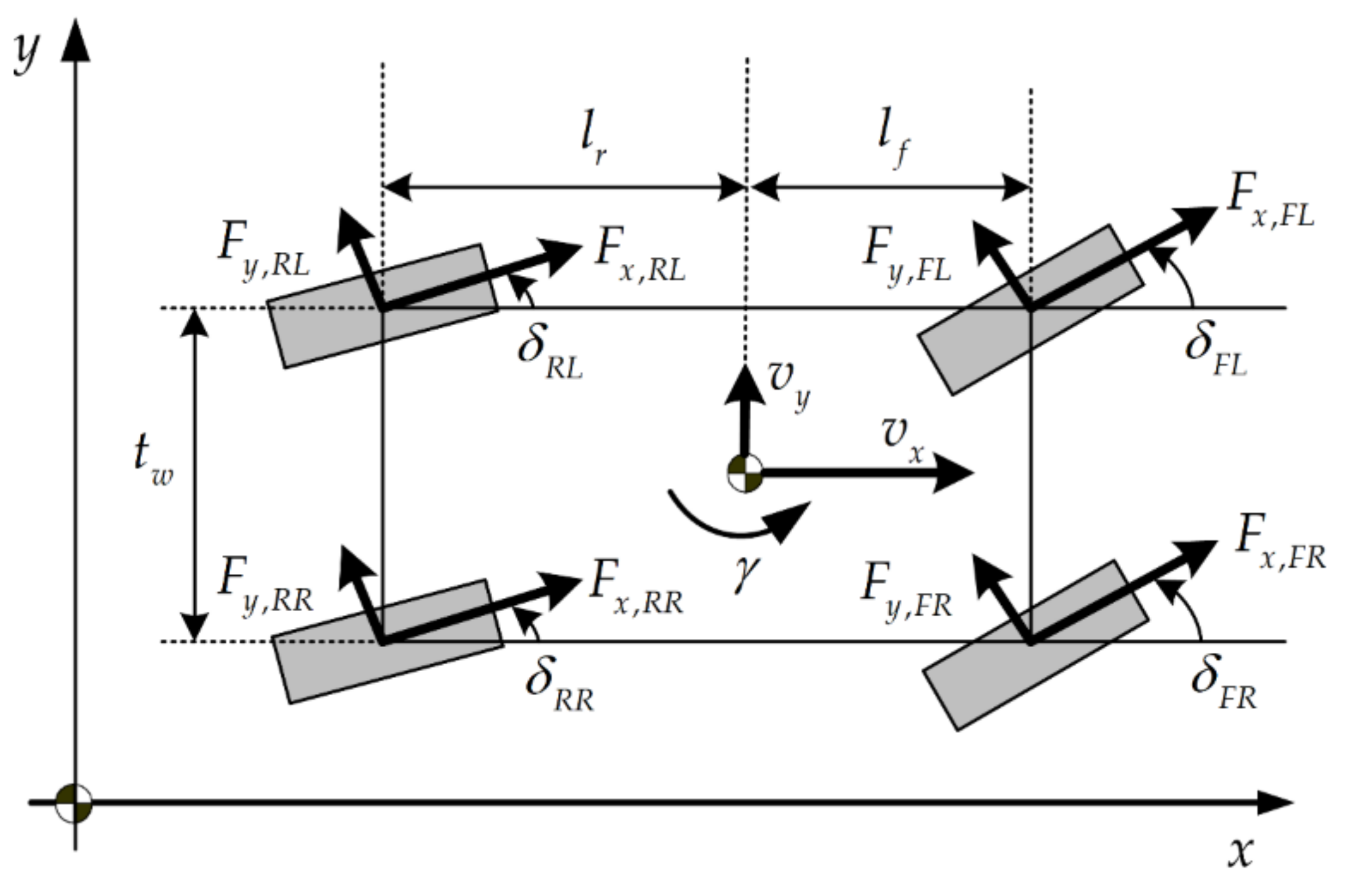
The remaining section of the paper is organized as follows: Section 2 describes the vehicle model used for controller design. The reference state decision for path and velocity tracking controllers are presented in Section 3. The linear time-varying MPC algorithm based on the local linearization of the vehicle model is presented in Section 4. The simulation results in the proposed algorithm and conventional ones are summarized in Section 5. The final section provides the conclusion and future works regarding the proposed algorithm.

2. Vehicle Model

The integrated control algorithm for path and velocity tracking control should consider the longitudinal, lateral, and yaw motion of the vehicle simultaneously. In other words, the equations of motion along the x-axis and y-axis, and around z-axis are defined to describe the behavior of the vehicle. Since it is assumed that the steering, driving, and braking of the four wheels are controlled independently, the longitudinal and lateral forces of each wheel should be considered as independent variables.

Figure 2 shows the free-body diagram of 4WIS/4WID vehicle model. Based on the variables as shown in Figure 2, the tire forces along the longitudinal and lateral directions generated by the steering and wheel torque were calculated. Then, the equations of the longitudinal (along x-direction), lateral (along y-direction), and yaw (around z-axis) motions are derived as (1), (2), and (3), respectively [55]. In these equations, M and I_z denote the total mass and the yaw moment of inertia of the vehicle, respectively. l_f and l_r are the distances of the front and rear axles from the CG, respectively. t_w is the track width of the vehicle. v_x and v_y are the longitudinal and lateral velocities of the vehicle, respectively. γ is the yaw rate. F_x,i, F_y,i and δ_i represent the longitudinal, lateral forces and the steering angle of each wheel, where i = FL, FR, RL, RR denote the front left, front right, rear left, and rear right wheels, respectively.

Longitudinal dynamics:

$$\begin{array}{ll}M{\dot{v}}_x=v_y\cdot \gamma & +F_{x,FL}\cdot \cos {\delta }_{FL}-F_{y,FL}\cdot \sin {\delta }_{FL}\hspace{0.17em}+F_{x,FR}\cdot \cos {\delta }_{FR}-F_{y,FR}\cdot \sin {\delta }_{FR}\\ & +F_{x,RL}\cdot \cos {\delta }_{RL}-F_{y,RL}\cdot \sin {\delta }_{RL}\hspace{0.17em}+F_{x,RR}\cdot \cos {\delta }_{RR}-F_{y,RR}\cdot \sin {\delta }_{RR}\end{array}$$

(1)

Lateral dynamics:

$$\begin{array}{ll}M{\dot{v}}_y=-v_x\cdot \gamma & +F_{x,FL}\cdot \sin {\delta }_{FL}+F_{y,FL}\cdot \cos {\delta }_{FL}+F_{x,FR}\cdot \sin {\delta }_{FR}+F_{y,FR}\cdot \cos {\delta }_{FR}\\ & +F_{x,RL}\cdot \sin {\delta }_{RL}+F_{y,RL}\cdot \cos {\delta }_{RL}\hspace{0.17em}+F_{x,RR}\cdot \sin {\delta }_{RR}+F_{y,RR}\cdot \cos {\delta }_{RR}\end{array}$$

(2)

Yaw dynamics:

$$\begin{array}{ll}{I}_z\dot{\gamma }=& l_f\left(F_{x,FL}\cdot \sin {\delta }_{FL}+F_{y,FL}\cdot \cos {\delta }_{FL}+F_{x,FR}\cdot \sin {\delta }_{FR}+F_{y,FR}\cdot \cos {\delta }_{FR}\right)\\ & -l_r\left(F_{x,RL}\cdot \sin {\delta }_{RL}+F_{y,RL}\cdot \cos {\delta }_{RL}+F_{x,RR}\cdot \sin {\delta }_{RR}+F_{y,RR}\cdot \cos {\delta }_{RR}\right)\\ & -0.5t_w\left(-F_{x,FL}\cdot \cos {\delta }_{FL}+F_{x,FR}\cdot \cos {\delta }_{FR}-F_{x,RL}\cdot \cos {\delta }_{RL}+F_{x,RR}\cdot \cos {\delta }_{RR}\right.\\ & \left.+F_{y,FL}\cdot \sin {\delta }_{FL}-F_{y,FR}\cdot \sin {\delta }_{FR}+F_{y,RL}\cdot \sin {\delta }_{RL}-F_{y,RR}\cdot \sin {\delta }_{RR}\right)\end{array}$$

(3)

The lateral tire force F_y,i of each wheel is modeled as a linear model under the assumption that the tire slip angle is small. Therefore, F_y,i can be represented as (4) where α_i is the slip angle of each tire. C_f and C_r are the cornering stiffness of the front and rear tires, respectively. Since the difference between the left and right tires is negligible compared to that of the front to rear tires, it is assumed that the cornering stiffness of the left and right tires are identical to each other.

$$\begin{array}{l}{F}_{y,FL}=C_f{\alpha }_{FL}=C_f\left({\delta }_{FL}-\frac{v_y+l_f\cdot \gamma }{v_x}\right),\hspace{1em}{F}_{y,FR}=C_f{\alpha }_{FR}=C_f\left({\delta }_{FR}-\frac{v_y+l_f\cdot \gamma }{v_x}\right)\\ F_{y,RL}=C_r{\alpha }_{RL}=C_r\left({\delta }_{RL}-\frac{v_y-l_r\cdot \gamma }{v_x}\right),\hspace{1em}{F}_{y,RR}=C_r{\alpha }_{RR}=C_r\left({\delta }_{RR}-\frac{v_y-l_r\cdot \gamma }{v_x}\right)\end{array}$$

(4)

where, α_i is the slip angle of each tire. C_f and C_r are the cornering stiffness of the front and rear tire, respectively. Since the difference of the left and right tire is negligible compared to the front-to-rear difference, it is assumed that the cornering stiffness of the left and right tires are identical to each other.

For the 4WID system, which is realized by using an in-wheel motor, F_x,i can be calculated as (5). In (5), I_w and w_i denote the wheel inertia and angular velocity of each wheel. T_i denotes the driving or braking torque of each wheel. R_e is the effective radius of the tire.

$$I_w{\dot{\omega }}_i=T_i-F_{x,i}{R}_e$$

(5)

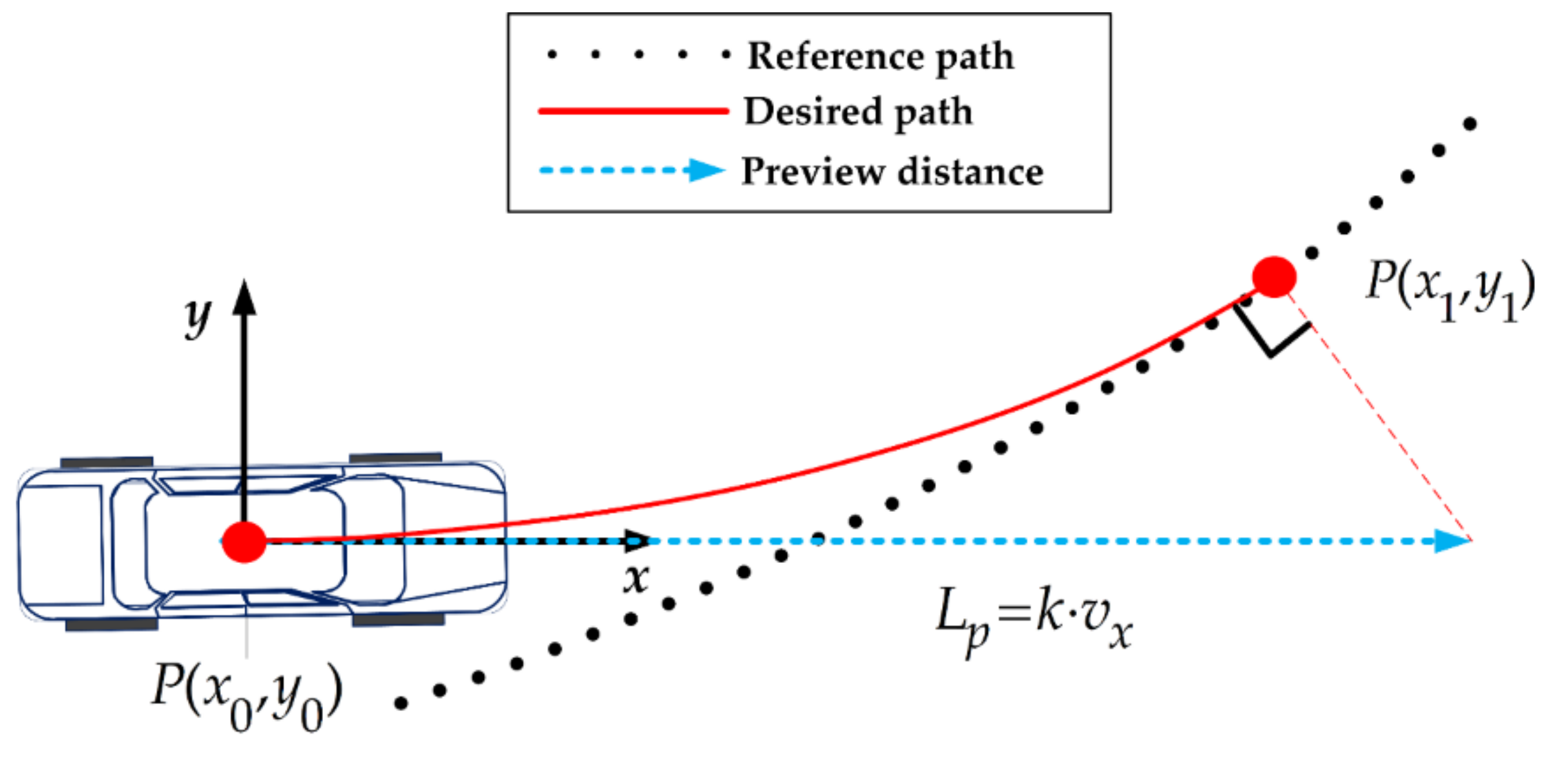
3. Reference State Decision

In the conventional approaches, path tracking controllers for autonomous vehicles have been designed by using the error dynamics based on the lateral position and heading errors with respect to the reference path [17,18,19,20,21,22,23,24,25]. In this paper, the pre-defined path that an autonomous vehicle wants to follow is called the reference path. To design the path tracking controller, several studies have converted the vehicle model to the path tracking one by considering the vehicle position and reference path [21,22,23]. However, when defining the plant model of the controller based on the error with respect to the reference path, it is difficult to intuitively connect the dynamic behavior of the vehicle to the errors. This is caused by the fact that an appropriate relationship between the lateral motion of vehicle and path tracking errors should be defined before deriving the path tracker. In addition, the dimension of the path tracking error is different from the yaw rate or the steering angle, which is closely related to the lateral motion of the vehicle [18,19,20]. Furthermore, the assumption on the reference path should be included in order to differentiate the error in constructing the error dynamics [20,21]. As a result, the path tracking performance may not be achieved in driving situations where the assumptions on the reference path are not valid. To overcome the limitations of the error dynamics, a reference state decision module is proposed for the purpose of determining the yaw rate and velocity profile within the prediction horizon.

The reference states, which consist of the reference yaw rate and the longitudinal velocity, have been determined when providing the reference path for MPC. Figure 3 shows the decision procedure of the desired path based on the reference one. First, the geometric relationship between the vehicle’s position and the reference path, which is depicted as a black dotted line in Figure 3, is considered. Under the assumption of low speed and negligible body slip angle, the required yaw rate needed to align the vehicle with the reference path is calculated by defining the desired path represented as a red solid line, which connects the center of gravity (C.G.) of the vehicle and the preview point on the reference path [56]. The C.G. of the vehicle and the preview point are denoted as P(x₀,y₀) and P(x₁,y₁), respectively. A preview length needed to define the preview point is determined by multiplying the preview time and the longitudinal velocity of the vehicle. In this paper, the preview time of 0.8 s is used to define the preview point. The preview length needed to determine P(x₁,y₁) is represented as L_p, and the preview time needed to calculate the L_p is denoted as gain k in Figure 3.

To determine the required yaw rate needed for a vehicle to follow the reference path, the curvature κ_des of the desired path should be defined first. Since the preview point is close enough to the vehicle, the desired path can be approximated by a simple polynomial. To define the desired path, the second-order polynomial, as given in (6), is adopted in this paper. This is defined with respect to the vehicle’s local coordinate system. The coefficients of (6), i.e., a, b and c, are determined with (7) by considering the position constraints at P(x₀,y₀), P(x₁,y₁) and the heading constraint at P(x₀,y₀). Based on the approximated desired path, κ_des at P(x₀,y₀) is derived as (8). Finally, the required yaw rate γ_j|k,input for path tracking is derived as (9). This is the explicit relationship between the required yaw rate and the reference path, which is the key contribution of this paper. By virtue of the relationship, vehicle chassis control dealing with the required yaw rate tracking and autonomous driving dealing with the reference path tracking are connected to each other.

$$y(x)=a{x}^2+bx+c$$

(6)

$$\left[\begin{array}{c}a\\ b\\ c\end{array}\right]={\left[\begin{array}{ccc}{x}_0^2& x_0& 1\\ x_1^2& x_1& 1\\ 2x_0& 1& 0\end{array}\right]}^{-1}\left[\begin{array}{c}{y}_0\\ y_1\\ y^{\prime }(x_0)\end{array}\right]$$

(7)

$${\kappa }_{des}=\frac{y^{″}\left(x_0\right)}{{\left\{1+y^{\prime }{\left(x_0\right)}^2\right\}}^{3/2}}=\frac{2a}{{\left\{1+{\left(2a{x}_0+b\right)}^2\right\}}^{3/2}}$$

(8)

$${\gamma }_{j|k,input}=v_{j|k}\cdot {\kappa }_{des}$$

(9)

Since the reference states for the MPC should be defined within the prediction horizon, it is necessary to distinguish the indices for the time and the prediction step. In (9), j is the prediction step index for reference state decision and k is the time index. Therefore, v_j|k means the j-th predicted longitudinal velocity at k-th time instant. For example, v_0|k is the current velocity of the vehicle at k-th instant.

The desired velocity v_j|k,des is defined by selecting the pre-defined velocity on the reference path. The pre-defined velocity on the reference path can be defined in various ways [29,30,31,57]. However, since the objective of this paper is to develop an integrated control algorithm for the path and velocity tracking controllers, the driving history of the driver is used to define the pre-defined velocity profiles and the reference path [15,58]. Then, a simple proportional controller is utilized to define the acceleration input for reference state decision, as given in (10).

$$a_{j|k,input}=-k\cdot \left(v_{j|k}-v_{j|k,des}\right)$$

(10)

As mentioned before, the reference states should be defined within the prediction horizon of the MPC. This means that the state prediction of the vehicle should be performed in order to define the reference states [10,52,53,54,58,59]. First, the state and input vectors of the motion prediction model is defined as (11). In (11), p_x,j|k, p_y,j|k, and θ_j|k are the longitudinal and lateral positions, and the yaw angle of the vehicle with respect to the local coordinate system defined at k-th time instant, respectively. v_j|k, γ_j|k, a_j|k, and γ′_j|k are the longitudinal velocity, the yaw rate, the longitudinal acceleration, and the yaw acceleration, respectively. When defining the state and input vectors, it is necessary to take the actuation delay of the vehicle into account. For this reason, the a_j|k, and γ’_j|k are defined separately with the virtual inputs, a_j|k,input, and γ_j|k,input in order to include the delay model in the reference state decision module.

$$\begin{array}{l}{x}_{pred,j|k}={[p_{x,j|k}\hspace{0.17em}\hspace{0.17em}\hspace{0.17em}{p}_{y,j|k}\hspace{0.17em}\hspace{0.17em}\hspace{0.17em}{\theta }_{j|k}\hspace{0.17em}\hspace{0.17em}\hspace{0.17em}{v}_{j|k}\hspace{0.17em}\hspace{0.17em}\hspace{0.17em}{\gamma }_{j|k}\hspace{0.17em}\hspace{0.17em}\hspace{0.17em}{a}_{j|k}\hspace{0.17em}\hspace{0.17em}\hspace{0.17em}{\gamma }_{j|k}^{\prime }]}^T\\ u_{j|k}={[{\gamma }_{j|k,input}\hspace{0.17em}\hspace{0.17em}\hspace{0.17em}{a}_{j|k,input}]}^T\end{array}$$

(11)

Under the assumption of small body slips, the kinematic model can be used to propagate the vehicle states. In addition, the lateral velocity is excluded from the state variable because of small body slip [39]. Based on the kinematic model, the prediction model is defined as (12). In (12), f(x_pred,j|k, u_j|k) is the non-linear equation, which is composed of the seven ones for each state variable, as given in (13). In (13), dt is the prediction sampling time, which is set to 0.1 s.

$$x_{pred,j+1|k}=f\left(x_{pred,j|k},u_{j|k}\right)$$

(12)

$$\begin{array}{l}{f}_1=p_{x,j|k}+v_{j|k}\cos {\theta }_{j|k}\cdot dt+\left(a_{j|k}\cos {\theta }_{j|k}-v_{j|k}\cdot {\gamma }_{j|k}\sin {\theta }_{j|k}\right)\cdot d{t}^2/2\\ f_2=p_{x,j|k}+v_{j|k}\cos {\theta }_{j|k}\cdot dt+\left(a_{j|k}\cos {\theta }_{j|k}-v_{j|k}\cdot {\gamma }_{j|k}\sin {\theta }_{j|k}\right)\cdot d{t}^2/2\\ f_3={\theta }_{j|k}+{\gamma }_{j|k}\cdot dt+{\dot{\gamma }}_{j|k}d{t}^2/2\\ f_4=v_{j|k}+a_{j|k}\cdot dt-k_a\cdot a_{j|k}\cdot d{t}^2/2\\ f_5={\gamma }_{j|k}+{\dot{\gamma }}_{j|k}\cdot dt-k_{\gamma }\cdot {\dot{\gamma }}_{j|k}\cdot d{t}^2/2\\ f_6=a_{j|k}-k_a\cdot a_{j|k}\cdot dt-k_a{}^2{a}_{j|k}\cdot d{t}^2/2+a_{j|k,input}\\ f_7={\dot{\gamma }}_{j|k}-k_{\gamma }\cdot {\dot{\gamma }}_{j|k}\cdot dt-k_{\gamma }{}^2{\dot{\gamma }}_{j|k}\cdot d{t}^2/2+{\gamma }_{j|k,input}.\end{array}$$

(13)

It is necessary to determine the longitudinal and lateral behaviors, which occur after the virtual inputs are applied, with the consideration of the actuation delay. If the virtual input is directly integrated by the prediction model without any considerations, the generated reference state can be the states that the actual vehicle cannot follow [59]. In this paper, the first-order delay model is used to describe the actuation delay in the prediction model. The expression of the first-order transfer function in the time domain appears as an exponential function, which is named as an exponential decay model in many studies [60]. Therefore, the exponential decay model is used in defining (13) in order to reflect the actuation delay in the prediction model. The exponential decay model is represented as (14) [60]. In (14), k_a and k_γ are the decay rate for the longitudinal acceleration and yaw rate, respectively. The values of k_a and k_γ are set to 0.05 and 0.15 for state prediction, respectively. a₀ and γ₀ are the initial values of the a_j|k, and γ_j|k, respectively.

$$\begin{array}{c}\dot{a}\left(k+j\cdot dt\right)=a_0\cdot \exp \left(-k_a\cdot \left(k+j\cdot dt\right)\right)\\ \dot{\gamma }\left(k+j\cdot dt\right)={\gamma }_0\cdot \exp \left(-k_{\gamma }\cdot \left(k+j\cdot dt\right)\right)\end{array}$$

(14)

The reference state x_ref,k is composed of v_x, v_y and γ. The reference v_x and γ are defined from the prediction results of v_j|k and γ_j|k, respectively. To minimize the body slip, the reference v_y is set to zero. Therefore, x_ref,k is defined as (15).

$$x{(k)}_{ref}=\left[\begin{array}{ccc}{v}_{1|k}& & v_{N_p|k}\\ 0& \cdots & 0\\ {\gamma }_{1|k}& & {\gamma }_{N_p|k}\end{array}\right]$$

(15)

4. Design of Linear Time-Varying Model Predictive Controller

The control algorithm for the over-actuated vehicle with 4WIS/4WID is designed with MPC. MPC has the advantage that an optimization has been performed for each moment while keeping future behavior in the account [9,10,48,49,50,51,52,59]. This advantage is realized by performing the optimization for a finite horizon and then optimizing repeatedly for every sampling time of the controller. In addition, since MPC is solved for every instant, prediction results of the plant and surrounding factors can be considered to respond to future events. For this reason, a linear time-varying MPC algorithm is proposed to control the over-actuated vehicle with 4WIS/4WID for the purpose of tracking the reference states. The details of the MPC algorithm will be discussed in the following sections.

4.1. Discretization and Linearization of the Vehicle Model

The vehicle model presented in Section 2 is the time-varying non-linear one. In the previous studies, various assumptions have been made to linearize the model and to transform it into a time-invariant one. In particular, small steering angle and constant velocity assumptions were frequently made to linearize a trigonometric function for steering inputs and to ensure the denominator divided by the velocity is constant [19,23,24]. In order to avoid the performance deterioration caused by the model linearization, the nonlinear control method has been introduced in designing the path and velocity tracking controllers [6,7,8,39,40,41,42,43,44,45]. Among the approaches using the non-linear control, a nonlinear MPC (NMPC) has been used to directly utilize the non-linear vehicle model. However, NMPC requires a complex nonlinear optimization algorithm to obtain optimal control inputs considering nonlinear prediction models, constraints, and cost functions. In addition, the complex numerical calculation of the NMPC increases the computational burden, which makes the NMPC solving sampling time larger [61]. Therefore, the non-linear vehicle model described in Section 2 is transformed to a linear time-varying one through local linearization.

The state and input vectors of the nonlinear vehicle model are defined as (16) and (17), respectively. After dividing (1) and (2) by M and (3) by I_z, the non-linear model can be expressed in the form of state-space equation with the definitions of (16) and (17). The state-space equation of the non-linear vehicle model is given in (18). In (18), the vehicle model is a continuous-time one. To adopt the model of (18) in the linear time-varying MPC controller, the model is needed to be linearized with respect to current states and inputs. The linearized model is obtained as (19) by approximation of (18) at x(t) and u(t − 1).

$$x={\left[\begin{array}{ccc}{v}_x& v_y& \gamma \end{array}\right]}^T$$

(16)

$$u={\left[\begin{array}{cccccccc}{\delta }_{FL}& {\delta }_{FR}& {\delta }_{RL}& {\delta }_{RR}& F_{x,FL}& F_{x,FR}& F_{x,RL}& F_{x,RR}\end{array}\right]}^T$$

(17)

$$\begin{array}{l}\dot{x}\left(t\right)=f\left(x\left(t\right),u\left(t\right)\right)\\ y\left(t\right)=h\left(x\left(t\right)\right)\end{array}$$

(18)

$$\begin{array}{l}\dot{x}\left(t\right)=A\left(t\right)x\left(t\right)+B\left(t\right)u\left(t\right)\\ y\left(t\right)=C\left(t\right)x\left(t\right)\end{array}$$

(19)

where,

$$A\left(t\right)={\left.\frac{\partial f\left(x\left(t\right),u\left(t\right)\right)}{\partial x}\right|}_{x\left(t\right),u\left(t-1\right)},\hspace{1em}B\left(t\right)={\left.\frac{\partial f\left(x\left(t\right),u\left(t\right)\right)}{\partial u}\right|}_{x\left(t\right),u\left(t-1\right)},\hspace{1em}C\left(t\right)={\left.\frac{\partial h\left(x\left(t\right)\right)}{\partial x}\right|}_{x\left(t\right)}$$

Since the 4WIS/4WID system uses a steering motor and IWM at each wheel, the steering angle and driving torque of each wheel are measurable. Therefore, C is the identity matrix of 8 × 8. The linear time-varying continuous system of (19) is discretized by first-order difference and transformed into (20). In (20), ∆T is the sampling time of the MPC algorithm, which is set to 0.1 s. n is the prediction step index for the MPC problem.

$$\begin{array}{l}x\left(n+1\right)=A_d\left(n\right)x\left(n\right)+B{\left(n\right)}_{d}u\left(n\right)\\ y\left(n\right)=C_{d}x\left(n\right)\end{array}$$

(20)

where,

$$A_d\left(n\right)=I+A\left(t\right)\Delta T,\hspace{1em}{B}_d\left(n\right)=B\left(t\right)\Delta T,\hspace{1em}{C}_d\left(n\right)=C\left(t\right)$$

4.2. Cost Function and Constraints

The objective of the controller designed for the over-actuated autonomous vehicle with 4WIS/4WID is to make the vehicle follow the reference path and velocity while minimizing the control effort. In order to achieve the objective of the proposed controller, the cost function of the MPC problem is defined as the quadratic form of (21). In (21), x(k)_ref is the reference states, which are defined in (15). α_i(n) and κ_i(n) are the tire slip angle and tire slip ratio for each wheel, respectively. The subscripts, i = 1, 2, 3, 4, correspond to FL, FR, RL, and RR tires of the vehicle. ρ is a relaxation factor used to avoid optimization failures when there is no optimal solution within the prediction horizon [50]. In other words, ρ ensure that at least cost function can find a suboptimal solution. In (21), Q and R are defined as (22), which represent the weighting matrices on reference tracking error and control input, respectively. In (22), Q_vx, Q_vy, and Q_γ are the weights on the tracking errors of the longitudinal and lateral velocities and the yaw rate, respectively. R_δ and R_Fx are the weighting matrices on the steering angle generated by 4WIS and the longitudinal force generated by the driving torques of 4WID at each wheel, respectively.

$$J={\displaystyle \sum _{n=1}^{N_p}\left({\left(x\left(n\right)-x{\left(n\right)}_{ref}\right)}^{T}Q\left(x\left(n\right)-x{\left(n\right)}_{ref}\right)+u{\left(n\right)}^{T}Ru\left(n\right)+{\displaystyle \sum _{i=1}^4{\alpha }_i}\left(n\right)+{\displaystyle \sum _{i=1}^4{\kappa }_i\left(n\right)}\right)}+\rho {\epsilon }^2$$

(21)

$$Q=\left[\begin{array}{ccc}{Q}_{vx}& & \\ & Q_{vy}& \\ & & Q_{\gamma }\end{array}\right],\hspace{1em}R={\left[\begin{array}{cccccc}{R}_{\delta }& & & & & \\ & \ddots & & & & \\ & & R_{\delta }& & & \\ & & & R_{Fx}& & \\ & & & & \ddots & \\ & & & & & R_{Fx}\end{array}\right]}_{\hspace{0.17em}8\times 8}$$

(22)

Equality constraints are derived from the vehicle model and initial condition of the optimization. In the MPC controller, the linearized and discretized vehicle models are used as a dynamic constraint, as given in (23). In (23), N_p is the number of the prediction steps. Then, the vehicle states at k-th time instant are used as initial condition constraints, as given in (24).

$$\begin{array}{l}x\left(n+1\right)=A_d\left(n\right)x\left(n\right)+B_d\left(n\right)u\left(n\right)\\ \hspace{0.17em}\hspace{0.17em}\hspace{0.17em}\hspace{0.17em}\hspace{0.17em}\hspace{0.17em}\hspace{0.17em}\hspace{0.17em}\hspace{0.17em}\hspace{0.17em}\hspace{0.17em}\hspace{0.17em}\hspace{0.17em}\hspace{0.17em}\hspace{0.17em}\hspace{0.17em}\hspace{0.17em}\hspace{0.17em}\hspace{0.17em}\hspace{0.17em}\hspace{0.17em}⋮\\ x\left(N_p\right)=A_d\left(N_p-1\right)x\left(N_p-1\right)+B_d\left(N_p-1\right)u\left(N_p-1\right)\end{array}$$

(23)

$$x_1\left(1\right)=v_{x,k},\hspace{0.17em}\hspace{0.17em}\hspace{0.17em}{x}_2\left(1\right)=v_{y,k},\hspace{0.17em}\hspace{0.17em}\hspace{0.17em}{x}_3\left(1\right)={\gamma }_k$$

(24)

Constraints on the states and inputs of MPC problem are defined as inequality ones in order to make the vehicle operate within a stable region. The constraints for the state vector of the MPC problem are defined as (25). The input constraints are defined as (26) and (27), which mean a maximum value and jerk limit to each actuator needed to consider the actuator limit. The inequality constraints on steering of 4WIS are defined as (26). In (26), δ_max and δ’_max are the maximum steering angle and its angular rate, respectively. The inequality constraints for drive torque of 4WID are defined as (27). In (27), F_x,max, and F’_x,max are the maximum longitudinal tire force and its rate, respectively. Finally, the parameters of the linear time-varying MPC are summarized in

Table 1. Parameters for model predictive control (MPC)-based controller.

Symbol	Values	Symbol	Values
Np	20 steps	vx,min	0 m/s
Qvx	1	vx,max	20 m/s
Qvy	2	vy,man	1 m/s
Qγ	40	δmax	30 deg
Rδ	0.1	δ′max	90 deg/s
RFx	0.001	Fx,max	1000 N
γmax	20 deg/s	F′x,max	4000 N/s

.

$$\hspace{0.17em}\begin{array}{c}\hspace{0.17em}\hspace{0.17em}\hspace{0.17em}\hspace{0.17em}\hspace{0.17em}{v}_{x,\min }\le x_1\left(n\right)\le v_{x,\max }\\ \hspace{0.17em}-v_{y,\max }\le x_2\left(n\right)\le v_{y,\max }\\ -{\gamma }_{\max }\le x_3\left(n\right)\le {\gamma }_{\max }\end{array}$$

(25)

$$\begin{array}{l}-{\delta }_{\max }\le u_i\left(n\right)\le {\delta }_{\max },\hspace{0.17em}\hspace{0.17em}\hspace{0.17em}\hspace{0.17em}\hspace{0.17em}\hspace{0.17em}\hspace{0.17em}\hspace{0.17em}\\ \left|u_i\left(n+1\right)-u_i\left(n\right)\right|\le {{\delta }^{\prime }}_{\max }\hspace{0.17em}\hspace{0.17em}\hspace{0.17em}\hspace{0.17em}\hspace{0.17em}\hspace{0.17em}\hspace{0.17em}\hspace{0.17em}i=1,2,3,4\end{array}$$

(26)

$$\begin{array}{l}-F_{x,\max }\le u_i\left(n\right)\le F_{x,\max },\hspace{0.17em}\\ \left|u_i\left(n+1\right)-u_i\left(n\right)\right|\le {F^{\prime }}_{x,\max },\hspace{0.17em}\hspace{0.17em}\hspace{0.17em}\hspace{0.17em}\hspace{0.17em}\hspace{0.17em}i=5,6,7,8\end{array}$$

(27)

5. Simulation

The simulation with the path and velocity tracking controllers was conducted to evaluate the performance of the proposed algorithm, comparing it with base algorithms. In this paper, two base algorithms were used to compare the performance of path and velocity tracking controllers. The details of the base algorithms and simulation environments are described in the following subsection.

5.1. Base Algorithms

As mentioned before, two base algorithms, Base #1 and Base #2, were adopted to compare the performance with the proposed algorithm. These algorithms were designed for 4WS with conventional 4WD vehicle systems. In other words, 4WS of the base algorithms control the left and right wheels with identical steering angles as done in the previous studies [4,5,6,8,36,38,39,40,41,42,43,44,45,46]. Base #1 is a simplified version of the proposed algorithm, which determines the FWS and RWS angles and a single driving torque. The diving torque determined by Base #1 is transferred to each wheel via a conventional drivetrain, which is composed of the transfer case, front, and rear differentials. Base #2 is based on the conventional RWS controller and velocity tracking algorithm [11]. The path tracking controller of Base #2 makes the RWS angle proportional to that of the FWS, which is determined by an adaptive steering controller. A model-free approach was adopted to track the reference yaw rate by determining the FWS angle. The reference yaw rate for Base #2 was determined by the same approach, as described in Section 3 [56]. Since the path tracking controller of Base #2 adapts the yaw rate gain by using the lateral position error to reference path, it can be applied to various kinds of vehicle [56]. The yaw rate gain represents the ratio between the steering angle and yaw rate. Therefore, the steering angle command can be determined without vehicle parameters and a detailed lateral model [56]. A similar model-free approach was also adopted to determine the throttle and brake inputs to track the reference velocity. The velocity tracking controller of Base #2 modeled the longitudinal behavior as a dynamic model with lumped parameters [62]. The lumped parameter was adapted to compensate for acceleration error in order to improve the velocity tracking performance. Therefore, the vehicle parameters are not required to determine the throttle and brake inputs [62].

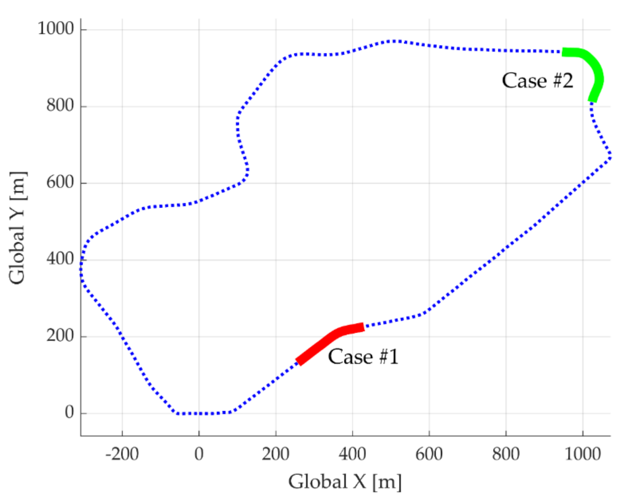
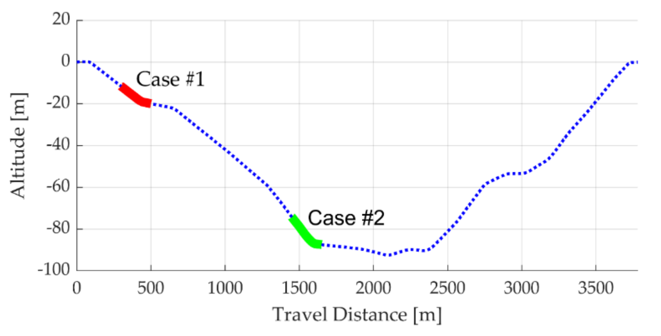
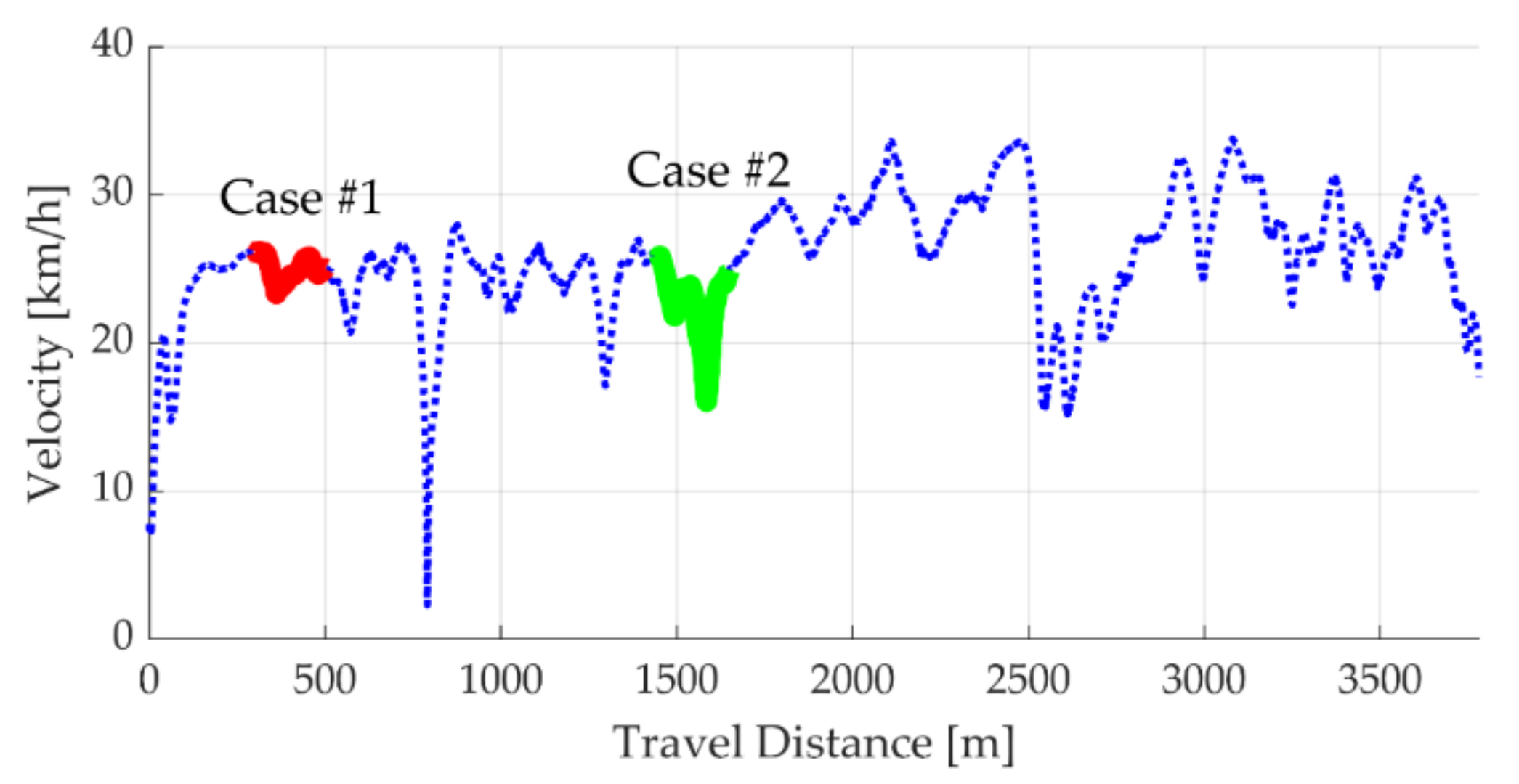
5.2. Simulation Environments

The co-simulation platform on MATLAB/Simulink and CarSim was adopted as the simulation environment. The proposed algorithm and Base #1 were implemented by using CVXGEN, which is a high-speed solver for a convex optimization problem [63]. For the Base #2, the MPC block was replaced by the base algorithm, and simulation was undertaken. In this paper, D-class sedan model given in CarSim was used as a vehicle model for simulation. The parameters used for simulation are listed in

Table 2. Parameters for the simulation study.

Symbol	Definition	Values
M	Vehicle Mass	1370 kg
lf	Distance of the front axle to the center of gravity	1.110 m
lr	Distance of the rear axle to the center of gravity	1.666 m
Iz	Vehicle yaw inertia	4192 kgm2
tw	Vehicle track width	1.795 m
Cf	Cornering stiffness of the front tires	77,388 N/rad
Cr	Cornering stiffness of the rear tires	77,388 N/rad
Np	Step of prediction horizon	20
ΔT	Sampling time of MPC	0.1 s

.

The campus road in the Seoul National University, Korea, was adopted as the reference path for the simulation. As shown in Figure 4, the reference path, which is approximately 3.7 km long, has a large curvature and steep slope region. In particular, this path includes a 90 deg turn and a section with a slope of about 15%. Therefore, the proposed reference path is an appropriate environment for evaluating the path tracking algorithm. Since the reference path given in Figure 4 and Figure 5 was acquired from a vehicle equipped with a high-precision DGPS, OxTS RT3002, not only the vehicle’s position but also the vehicle’s pose and dynamic states were precisely collected. The velocity history of the human driving data was used to define the reference velocity on the reference path, as shown in Figure 6. Among all simulation results, the results of Case #1 with a slight slope and curvature and Case #2 with 90 deg turning on a steep slope are summarized in the following section. The road sections of Case #1 and Case #2 are marked in red and green bold lines in Figure 4, Figure 5 and Figure 6, respectively.

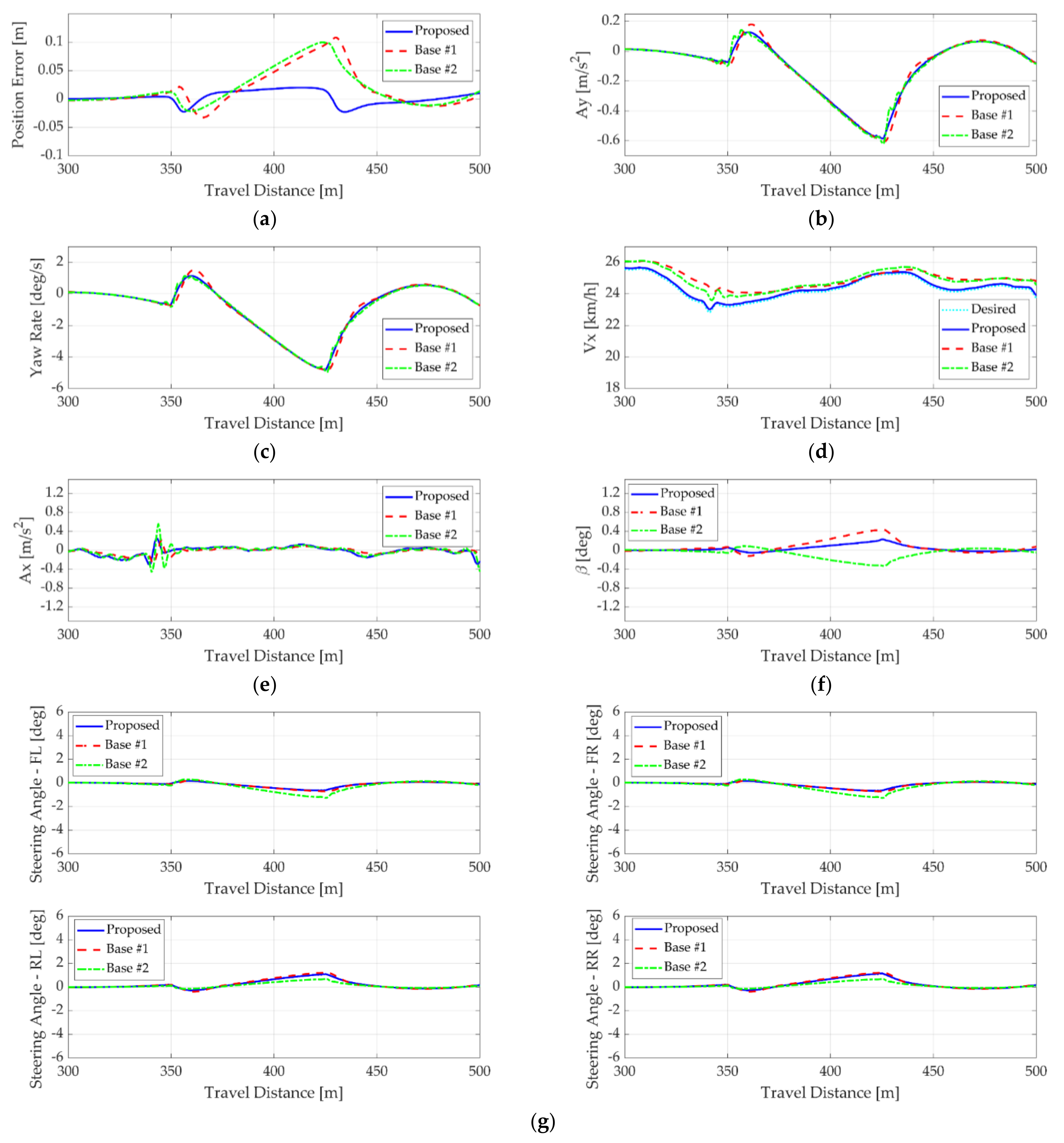
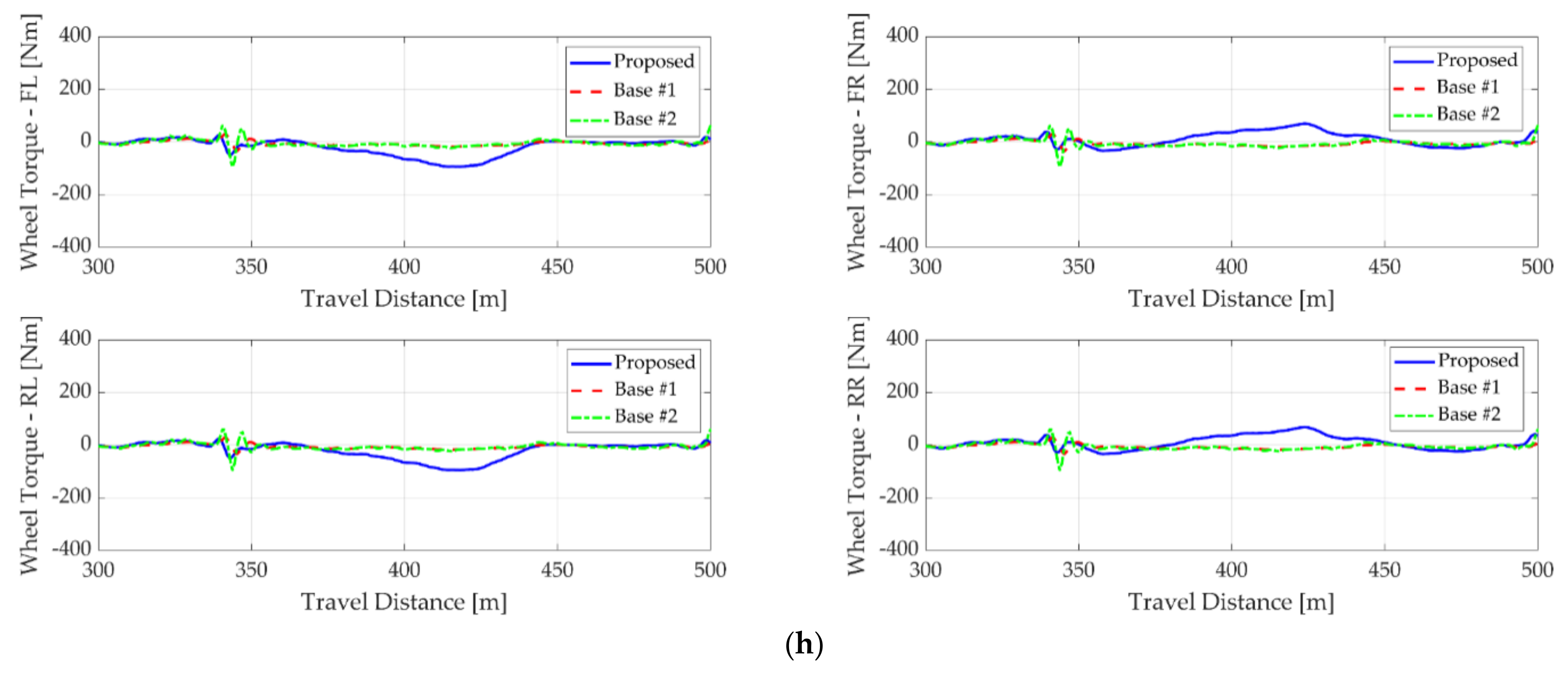
5.3. Simulation Results

The simulation results of the proposed and base algorithms for Case #1 are summarized in Figure 7. In Figure 7, the results of the proposed algorithm, Base #1, and Base #2 are depicted as a blue solid, red dashed and green dash-dot lines, respectively. In addition, the desired velocity is marked as a cyan dotted line in Figure 7b. Since the simulation time of each algorithm is different, the simulation histories are described with respect to the travel distance of the closest point on the reference path.

As shown in Figure 7a, simulation results of Case #1 show that the position error of the proposed algorithm was maintained below 0.05 m. Meanwhile, the position errors of Base #1 and Base #2 were almost three times that of the proposed one, and even the lateral acceleration and the yaw rate were almost the same for all algorithms in Figure 7b,c. For longitudinal motion, the velocity tacking performances of Base #1 and Base #2 showed an error of about 1 km/h, as shown in Figure 7d. In addition, a larger jerk occurred in the case of the base algorithms in Figure 7e. As shown in Figure 7h, Base #1 and Base #2 evenly distributed the driving torque through the conventional drivetrain, which causes a larger body slip angle than the proposed algorithm. Since Base #2 determined the RWS angle in proportion to that of the FWS as shown in Figure 7g, it caused the largest body slip among the simulation results, as shown in Figure 7f. Moreover, the proposed algorithm generated the additional lateral moment by actively distributing the driving torque to each wheel, as shown in Figure 7h. From the results, the proposed algorithm showed the most accurate path and velocity tracking performance than the base algorithms while regulating the body slip angle.

The simulation results of Case #2 are summarized in Figure 8. Simulation for Case #2 included a larger curvature and steep road slope than Case #1, which makes it difficult for the vehicle to track the reference path and velocity. Like simulation Case #1, the proposed algorithm improved the path and velocity tracking performances, compared to Base #1 and Base #2, as shown in Figure 8a,d. As shown in Figure 8b,c, all algorithms showed the similar histories of lateral acceleration and yaw rate. In terms of the reference tracking performance, the proposed algorithm prevented the position error from increasing by actively distributing the driving and braking torques to each wheel, as shown in Figure 8h. In the case of Base #1, the steering angle was determined similarly with that of the proposed algorithm, as shown in Figure 8g. However, the driving torque was not effectively distributed, compared to the proposed algorithm. Consequently, the path tracking performance of Base #1 was not improved as much as Base #2, as shown in Figure 8a. For Base #2, severe jerks in longitudinal acceleration and driving torque occurred, as shown in Figure 8e,h. This was caused by the fact that the proposed algorithm and Base #1, which are based on the MPC, predict and consider the road conditions ahead for optimization. Meanwhile, the longitudinal controller of Base #2 only takes the current states into account to determine the control inputs. In addition, since Base #2 was not designed to consider the lateral velocity, it can be seen that the body slip was not properly managed, compared to the proposed algorithm, as shown in Figure 8f.

From the perspective of energy consumption, it can be considered that more energy is consumed in applying the proposed algorithm because the wheel torque was highly used. However, considering that regenerative braking is available in a vehicle with IWM, all three algorithms can be found to be at the same level of energy consumption. For example, as shown in Figure 8h, the acceleration torque was used for the left wheels, but the right wheels were decelerating to a similar level of the acceleration torque on the left. Therefore, there were no significant differences in energy consumption from the base algorithms because regenerative braking can recover similar levels of energy used to drive left wheels. Therefore, it can be concluded that the proposed algorithm improves the path and velocity tracking performances for the autonomous vehicle with 4WIS/4WID without much loss in energy consumption.

6. Conclusions

This paper proposed a new algorithm for the integrated path and velocity tracking controller for an autonomous vehicle with 4WIS/4WID. The proposed algorithm is composed of the two modules: a reference state decision and MPC-based motion controller. The reference state decision module determines the reference yaw rate and velocity profiles to provide the reference state for the MPC algorithm. The MPC-based motion controller was designed based on the linear time-varying vehicle model in order to handle the high curvature road conditions which require a large steering angle. The local linearization of the non-linear vehicle model was performed for every sampling step to minimize the modeling error caused by linearization and discretization. The MPC was used to optimize and allocate the control inputs while reducing the computational load compared to non-linear MPC.

The performance of the proposed algorithm was evaluated via simulation conducted on the co-simulation environment, MATLAB/Simulink and CarSim. The reference path and velocity were defined by collecting the driving data of the driver from real driving experiments. The simulation results showed that the proposed algorithm achieved improved reference tracking performance than the base algorithms, which were based on the simplified MPC-based controller and adaptive control approach, respectively. Future work will consider extreme driving conditions, such as racing or the split-mu condition. The scope of the proposed algorithm will be extended toward the fault-tolerant control approach to over-actuated vehicle systems in order to guarantee the safety of autonomous vehicles.

References

1. Paden, B.; Cap, M.; Yong, S.Z.; Yershov, D.; Frazzoli, E. A Survey of Motion Planning and Control Techniques for Self-Driving Urban Vehicles. IEEE Trans. Intell. Veh. 2016, 1, 33–55. [Google Scholar] [CrossRef] [Green Version]
2. Yurtsever, E.; Lambert, J.; Carballo, A.; Takeda, K. A survey of autonomous driving: Common practices and emerging technologies. IEEE Access 2020, 8, 58443–58469. [Google Scholar] [CrossRef]
3. Aguiar, A.; Dos Santos, F.; Cunha, J.; Sobreira, H.; Sousa, A. Localization and Mapping for Robots in Agriculture and Forestry: A Survey. Robotics 2020, 9, 97. [Google Scholar] [CrossRef]
4. Wang, J.; Wang, R.; Jing, H.; Chen, N. Coordinated Active Steering and Four-Wheel Independently Driving/Braking Control with Control Allocation. Asian J. Control 2015, 18, 98–111. [Google Scholar] [CrossRef]
5. Chen, X.; Peng, Y.; Hang, P.; Tang, T. Path tracking control of four-wheel independent steering electric vehicles based on optimal control. In Proceedings of the 2020 39th Chinese Control Conference (CCC), Shenyang, China, 27–29 July 2020; pp. 5436–5442. [Google Scholar]
6. Hang, P.; Chen, X.; Luo, F. LPV/H∞ Controller Design for Path Tracking of Autonomous Ground Vehicles Through Four-Wheel Steering and Direct Yaw-Moment Control. Int. J. Automot. Technol. 2019, 20, 679–691. [Google Scholar] [CrossRef]
7. Hiraoka, T.; Nishihara, O.; Kumamoto, H. Automatic path-tracking controller of a four-wheel steering vehicle. Veh. Syst. Dyn. 2009, 47, 1205–1227. [Google Scholar] [CrossRef]
8. Hu, C.; Wang, R.; Yan, F. Integral Sliding Mode-Based Composite Nonlinear Feedback Control for Path Following of Four-Wheel Independently Actuated Autonomous Vehicles. IEEE Trans. Transp. Electrif. 2016, 2, 221–230. [Google Scholar] [CrossRef]
9. Tan, Q.; Dai, P.; Zhang, Z.; Katupitiya, J. MPC and PSO Based Control Methodology for Path Tracking of 4WS4WD Vehicles. Appl. Sci. 2018, 8, 1000. [Google Scholar] [CrossRef] [Green Version]
10. Tan, Q.; Wang, X.; Taghia, J.; Katupitiya, J. Force control of two-wheel-steer four-wheel-drive vehicles using model predictive control and sequential quadratic programming for improved path tracking. Int. J. Adv. Robot. Syst. 2017, 14, 1729881417746295. [Google Scholar] [CrossRef] [Green Version]
11. Park, K.; Joa, E.; Yi, K.; Yoon, Y. Rear-Wheel Steering Control for Enhanced Steady-State and Transient Vehicle Handling Characteristics. IEEE Access 2020, 8, 149282–149300. [Google Scholar] [CrossRef]
12. Hang, P.; Chen, X. Integrated chassis control algorithm design for path tracking based on four-wheel steering and direct yaw-moment control. Proc. Inst. Mech. Eng. Part I J. Syst. Control. Eng. 2019, 233, 625–641. [Google Scholar] [CrossRef]
13. Yim, S.; Park, Y.; Yi, K. Design of active suspension and electronic stability program for rollover prevention. Int. J. Automot. Technol. 2010, 11, 147–153. [Google Scholar] [CrossRef]
14. Woo, S.; Cha, H.; Yi, K.; Jang, S. Active Differential Control for Improved Handling Performance of Front-Wheel-Drive High-Performance Vehicles. Int. J. Automot. Technol. 2021, 22, 537–546. [Google Scholar] [CrossRef]
15. Kim, K.; Kim, B.; Lee, K.; Ko, B.; Yi, K. Design of Integrated Risk Management-Based Dynamic Driving Control of Automated Vehicles. IEEE Intell. Transp. Syst. Mag. 2017, 9, 57–73. [Google Scholar] [CrossRef]
16. Yoo, J.M.; Jeong, Y.; Yi, K. Virtual Target-Based Longitudinal Motion Planning of Autonomous Vehicles at Urban Intersections: Determining Control Inputs of Acceleration with Human Driving Characteristic-Based Constraints. IEEE Veh. Technol. Mag. 2021, 16, 38–46. [Google Scholar] [CrossRef]
17. Snider, J.M. Automatic Steering Methods for Autonomous Automobile Path Tracking; CMU-RITR-09-08; Robotics Institute: Pittsburgh, PA, USA, 2009. [Google Scholar]
18. Wang, W.-J.; Hsu, T.-M.; Wu, T.-S. The improved pure pursuit algorithm for autonomous driving advanced system. In Proceedings of the 2017 IEEE 10th International Workshop on Computational Intelligence and Applications, Hiroshima, Japan, 11–12 November 2017; pp. 33–38. [Google Scholar]
19. Elbanhawi, M.; Simic, M.; Jazar, R. Receding horizon lateral vehicle control for pure pursuit path tracking. J. Vib. Control 2016, 24, 619–642. [Google Scholar] [CrossRef]
20. Amer, N.H.; Zamzuri, H.; Hudha, K.; Aparow, V.R.; Abd Kadir, Z.; Abidin, A.F.Z. Path tracking controller of an autonomous armoured vehicle using modified Stanley controller optimized with particle swarm optimization. J. Braz. Soc. Mech. Sci. Eng. 2018, 40, 104. [Google Scholar] [CrossRef]
21. Piao, C.; Liu, X.; Lu, C. Lateral control using parameter self-tuning LQR on autonomous vehicle. In Proceedings of the 2019 International Conference on Intelligent Computing, Automation and Systems, Chongqing, China, 6–8 December 2019; pp. 913–917. [Google Scholar]
22. Zhang, C.; Hu, J.; Qiu, J.; Yang, W.; Sun, H.; Chen, Q. A Novel Fuzzy Observer-Based Steering Control Approach for Path Tracking in Autonomous Vehicles. IEEE Trans. Fuzzy Syst. 2018, 27, 278–290. [Google Scholar] [CrossRef]
23. Raffo, G.; Gomes, G.K.; Normey-Rico, J.E.; Kelber, C.R.; Becker, L.B. A Predictive Controller for Autonomous Vehicle Path Tracking. IEEE Trans. Intell. Transp. Syst. 2009, 10, 92–102. [Google Scholar] [CrossRef]
24. Sun, C.; Zhang, X.; Xi, L.; Tian, Y. Design of a Path-Tracking Steering Controller for Autonomous Vehicles. Energies 2018, 11, 1451. [Google Scholar] [CrossRef] [Green Version]
25. Bai, G.; Meng, Y.; Liu, L.; Luo, W.; Gu, Q.; Li, K. A New Path Tracking Method Based on Multilayer Model Predictive Control. Appl. Sci. 2019, 9, 2649. [Google Scholar] [CrossRef] [Green Version]
26. Jiang, L.; Wang, Y.; Wang, L.; Wu, J. Path tracking control based on Deep reinforcement learning in Autonomous driving. In Proceedings of the 2019 3rd Conference on Vehicle Control and Intelligence, Hefei, China, 21–22 September 2019; pp. 1–6. [Google Scholar]
27. Song, S.; Chen, H.; Sun, H.; Liu, M. Data Efficient Reinforcement Learning for Integrated Lateral Planning and Control in Automated Parking System. Sensors 2020, 20, 7297. [Google Scholar] [CrossRef] [PubMed]
28. Kamran, D.; Zhu, J.; Lauer, M. Learning path tracking for real car-like mobile robots from simulation. In Proceedings of the 2019 European Conference on Mobile Robots, Prague, Czech Republic, 4–6 September 2019; pp. 1–6. [Google Scholar]
29. Yan, W.; Li, C.; Huang, Y.; Yang, L. Smart Longitudinal Velocity Control of Autonomous Vehicles in Interactions with Distracted Human-Driven Vehicles. IEEE Access 2019, 7, 168060–168074. [Google Scholar] [CrossRef]
30. Bianco, C.G.L.; Romano, M. Optimal velocity planning for autonomous vehicles considering curvature constraints. In Proceedings of the 2007 IEEE International Conference on Robotics and Automation, Rome, Italy, 10–14 April 2007; pp. 2706–2711. [Google Scholar]
31. Lefevre, S.; Carvalho, A.; Borrelli, F. A Learning-Based Framework for Velocity Control in Autonomous Driving. IEEE Trans. Autom. Sci. Eng. 2015, 13, 32–42. [Google Scholar] [CrossRef]
32. Alfi, A.; Farrokhi, M. Hybrid state-feedback sliding-mode controller using fuzzy logic for four-wheel-steering vehicles. Veh. Syst. Dyn. 2009, 47, 265–284. [Google Scholar] [CrossRef]
33. Chen, C.; Jia, Y.; Du, J.; Yu, F. Lane keeping control for autonomous 4WS4WD vehicles subject to wheel slip constraint. In Proceedings of the 2012 American Control Conference, Montreal, QC, Canada, 27–29 June 2012; pp. 6515–6520. [Google Scholar]
34. Enache, N.M.; Guegan, S.; Desnoyer, F.; Vorobieva, H. Lane keeping and lane departure avoidance by rear wheels steering. In Proceedings of the 2012 IEEE Intelligent Vehicles Symposium, Madrid, Spain, 3–7 June 2012; pp. 359–364. [Google Scholar]
35. Oya, M.; Wang, Q. Adaptive lane keeping controller for four-wheel-steering vehicles. In Proceedings of the 2007 IEEE International Conference on Control and Automation, Guangzhou, China, 30 May–1 June 2007; pp. 1942–1947. [Google Scholar]
36. Galvani, M.; Biral, F.; Nguyen, B.M.; Fujimoto, H. Four wheel optimal autonomous steering for improving safety in emergency collision avoidance manoeuvres. In Proceedings of the 2014 IEEE 13th international Workshop on Advanced Motion Control, Yokohama, Japan, 14–16 March 2014; pp. 362–367. [Google Scholar]
37. Raksincharoensak, P.; Nagai, M.; Mouri, H. Investigation of automatic path tracking control using four-wheel steering vehicle. In Proceedings of the IEEE International Vehicle Electronics Conference 2001, Tottori, Japan, 25–28 September 2001; pp. 73–77. [Google Scholar]
38. Hu, C.; Wang, R.; Yan, F.; Chen, N. Output constraint control on path following of four-wheel independently actuated autonomous ground vehicles. IEEE Trans. Veh. Technol. 2015, 65, 4033–4043. [Google Scholar] [CrossRef]
39. Shu, P.; Sagara, S.; Wang, Q.; Oya, M. Improved adaptive lane-keeping control for four-wheel steering vehicles without lateral velocity measurements. Int. J. Robust Nonlinear Control 2017, 27, 4154–4168. [Google Scholar] [CrossRef]
40. Yoshida, Y.; Wang, Q.; Oya, M.; Okumura, K. Adaptive longitudinal velocity and lane keeping control of four-wheel-steering vehicles. In Proceedings of the SICE Annual Conference 2007, Takamatsu, Japan, 17–20 September 2007; pp. 1305–1310. [Google Scholar]
41. Wu, J.; Wang, Z.; Zhang, L. Unbiased-estimation-based and computation-efficient adaptive MPC for four-wheel-independently-actuated electric vehicles. Mech. Mach. Theory 2020, 154, 104100. [Google Scholar] [CrossRef]
42. Ding, X.; Wang, Z.; Zhang, L. Hybrid Control-Based Acceleration Slip Regulation for Four-Wheel-Independent-Actuated Electric Vehicles. IEEE Trans. Transp. Electrif. 2021, 7, 1976–1989. [Google Scholar] [CrossRef]
43. Solea, R.; Filipescu, A.; Filipescu, S.; Dumitrascu, B. Sliding-mode controller for four-wheel-steering vehicle: Trajectory-tracking problem. In Proceedings of the 2010 8th World Congress on Intelligent Control and Automation, Jinan, China, 7–9 July 2010; pp. 1185–1190. [Google Scholar]
44. Hu, C.; Qin, Y.; Cao, H.; Song, X.; Jiang, K.; Rath, J.J.; Wei, C. Lane keeping of autonomous vehicles based on differential steering with adaptive multivariable super-twisting control. Mech. Syst. Signal Process. 2019, 125, 330–346. [Google Scholar] [CrossRef]
45. Kasahara, M.; Kanai, Y.; Mori, Y. Adjust method of nonlinear gain in four-wheel steering control using Sliding Mode Control. In Proceedings of the 2009 4th IEEE Conference on Industrial Electronics and Applications, Xi’an, China, 25–27 May 2009; pp. 608–613. [Google Scholar]
46. Wang, R.; Yin, G.; Jin, X. Robust adaptive sliding mode control for nonlinear four-wheel steering autonomous Vehicles path tracking systems. In Proceedings of the 2016 IEEE 8th International Power Electronics and Motion Control Conference, Hefei, China, 22–26 May 2016; pp. 2999–3006. [Google Scholar]
47. Hang, P.; Luo, F.; Fang, S.; Chen, X. Path tracking control of a four-wheel-independent-steering electric vehicle based on model predictive control. In Proceedings of the 2017 36th Chinese Control Conference (CCC), Dalian, China, 26–28 July 2017; pp. 9360–9366. [Google Scholar]
48. Fnadi, M.; Plumet, F.; Benamar, F. Model predictive control based dynamic path tracking of a four-wheel steering mobile robot. In Proceedings of the 2019 IEEE/RSJ International Conference on Intelligent Robots and Systems, Macau, China, 3–8 November 2019; pp. 4518–4523. [Google Scholar]
49. Liang, Y.; Li, Y.N.; Khajepour, A.; Zheng, L. Holistic Adaptive Multi-Model Predictive Control for the Path Following of 4WID Autonomous Vehicles. IEEE Trans. Veh. Technol. 2021, 70, 69–81. [Google Scholar] [CrossRef]
50. Wu, H.; Li, Z.; Si, Z. Trajectory tracking control for four-wheel independent drive intelligent vehicle based on model predictive control and sliding mode control. Adv. Mech. Eng. 2020, 13, 16878140211045142. [Google Scholar] [CrossRef]
51. Yu, Y.; Li, Y.; Liang, Y.; Zheng, L.; Ren, Y. Decoupling motion tracking control for 4WD autonomous vehicles based on the path correction. Proc. Inst. Mech. Eng. Part D J. Automob. Eng. 2021, 09544070211015928. [Google Scholar] [CrossRef]
52. An, Q.; Cheng, S.; Li, C.; Li, L.; Peng, H. Game Theory-Based Control Strategy for Trajectory Following of Four-Wheel Independently Actuated Autonomous Vehicles. IEEE Trans. Veh. Technol. 2021, 70, 2196–2208. [Google Scholar] [CrossRef]
53. Liu, C.; Lee, S.; Varnhagen, S.; Tseng, H.E. Path planning for autonomous vehicles using model predictive control. In Proceedings of the 2017 IEEE Intelligent Vehicles Symposium, Los Angeles, CA, USA, 11–14 June 2017; pp. 174–179. [Google Scholar]
54. Baskar, L.D.; De Schutter, B.; Hellendoorn, H. Model-based predictive traffic control for intelligent vehicles: Dynamic speed limits and dynamic lane allocation. In Proceedings of the 2008 IEEE Intelligent Vehicles Symposium, Eindhoven, The Netherlands, 4–6 June 2008; pp. 174–179. [Google Scholar]
55. Li, D.-Y.; Song, Y.-D.; Huang, D.; Chen, H.-N. Model-Independent Adaptive Fault-Tolerant Output Tracking Control of 4WS4WD Road Vehicles. IEEE Trans. Intell. Transp. Syst. 2012, 14, 169–179. [Google Scholar] [CrossRef]
56. Jung, C.; Kim, H.; Son, Y.; Lee, K.; Yi, K. Parameter adaptive steering control for autonomous driving. In Proceedings of the 17th International IEEE Conference on Intelligent Transportation Systems, Qingdao, China, 8–11 October 2014; pp. 1462–1467. [Google Scholar]
57. Hermand, E.; Nguyen, T.W.; Hosseinzadeh, M.; Garone, E. Constrained control of UAVs in geofencing applications. In Proceedings of the 2018 26th Mediterranean Conference on Control and Automation, Zadar, Croatia, 19–22 June 2018; pp. 217–222. [Google Scholar]
58. Kim, B.; Kim, D.; Park, S.; Jung, Y.; Yi, K. Automated Complex Urban Driving based on Enhanced Environment Representation with GPS/map, Radar, Lidar and Vision. IFAC-PapersOnLine 2016, 49, 190–195. [Google Scholar] [CrossRef]
59. Jeong, Y. Self-Adaptive Motion Prediction-Based Proactive Motion Planning for Autonomous Driving in Urban Environments. IEEE Access 2021, 9, 105612–105626. [Google Scholar] [CrossRef]
60. Kim, B.; Yi, K. Probabilistic and Holistic Prediction of Vehicle States Using Sensor Fusion for Application to Integrated Vehicle Safety Systems. IEEE Trans. Intell. Transp. Syst. 2014, 15, 2178–2190. [Google Scholar] [CrossRef]
61. Chen, W.-H.; O’Reilly, J.; Ballance, D. Model predictive control of nonlinear systems: Computational burden and stability. IEE Proc. Control Theory Appl. 2000, 147, 387–394. [Google Scholar] [CrossRef] [Green Version]
62. Kim, H.; Yi, K. Combined throttle and brake control for vehicle cruise control: A model free approach. In Proceedings of the 2013 IEEE Intelligent Vehicles Symposium (IV), Gold Coast, Australia, 23–26 June 2013; pp. 859–864. [Google Scholar]
63. Mattingley, J.; Boyd, S. CVXGEN: A code generator for embedded convex optimization. Optim. Eng. 2011, 13, 1–27. [Google Scholar] [CrossRef]
Figure 1. Schematic diagram of the proposed algorithm.
Electronics 10 02812 g001
Figure 2. Free-body diagram of four-wheel independent steering/four-wheel independently driving (4WIS/4WID) vehicle model.
Electronics 10 02812 g002
Figure 3. Desired path decision based on the reference.
Electronics 10 02812 g003
Figure 4. Reference paths with Case #1 and Case #2.
Electronics 10 02812 g004
Figure 5. Altitude of reference path with Case #1 and Case #2.
Electronics 10 02812 g005
Figure 6. Reference velocity with Case #1 and Case #2.
Electronics 10 02812 g006
Figure 7. Simulation results of Case #1: (a) position error; (b) lateral acceleration; (c) yaw rate; (d) longitudinal velocity; (e) longitudinal acceleration; (f) body slip angle; (g) steering angle; (h) wheel torque.
Electronics 10 02812 g007aElectronics 10 02812 g007b
Figure 8. Simulation results of Case #2: (a) Position error; (b) lateral acceleration; (c) yaw rate; (d) longitudinal velocity; (e) longitudinal acceleration; (f) body slip angle; (g) steering angle; (h) wheel torque.
Electronics 10 02812 g008