
Sentiment Analysis in Twitter Based on Knowledge Graph and Deep Learning Classification


1
Department of Computer Science, Universidad Simón Bolívar, Caracas 1080, Venezuela
2
Centre for Environmental Research, Helmholtz Department of Molecular Systems Biology, 04318 Leipzig, Germany
*
Authors to whom correspondence should be addressed.
Electronics 2021, 10(22), 2739; https://doi.org/10.3390/electronics10222739
Submission received: 4 October 2021
/
Revised: 16 October 2021
/
Accepted: 21 October 2021
/
Published: 10 November 2021
(This article belongs to the Special Issue Deep Learning and Explainability for Sentiment Analysis)
Abstract
:The traditional way to address the problem of sentiment classification is based on machine learning techniques; however, these models are not able to grasp all the richness of the text that comes from different social media, personal web pages, blogs, etc., ignoring the semantic of the text. Knowledge graphs give a way to extract structured knowledge from images and texts in order to facilitate their semantic analysis. This work proposes a new hybrid approach for Sentiment Analysis based on Knowledge Graphs and Deep Learning techniques to identify the sentiment polarity (positive or negative) in short documents, such as posts on Twitter. In this proposal, tweets are represented as graphs; then, graph similarity metrics and a Deep Learning classification algorithm are applied to produce sentiment predictions. This approach facilitates the traceability and interpretability of the classification results, thanks to the integration of the Local Interpretable Model-agnostic Explanations (LIME) model at the end of the pipeline. LIME allows raising trust in predictive models, since the model is not a black box anymore. Uncovering the black box allows understanding and interpreting how the network could distinguish between sentiment polarities. Each phase of the proposed approach conformed by pre-processing, graph construction, dimensionality reduction, graph similarity, sentiment prediction, and interpretability steps is described. The proposal is compared with character n-gram embeddings-based Deep Learning models to perform Sentiment Analysis. Results show that the proposal is able to outperforms classical n-gram models, with a recall up to 89% and F1-score of 88%.
1. Introduction
Users of social networks make use of such platforms to express opinions as well as emotions on any topic. Twitter, one of the most used, is a social network and a microblogging service that allows users to write small pieces of text or messages known as tweets, through which users can interact with each other and express their ideas. In this context, Sentiment Analysis models have demonstrated efficiency in predicting feelings in texts and to determine users’ perception of aspects of everyday life [1]. The information extracted by Sentiment Analysis can be used as knowledge for further analysis. In general, the idea is to predict the results or trends of a particular topic based on sentiment [2], for example in contexts of product preferences in the market [3,4], film preferences [5], or political opinions [6].
However, on Twitter, predicting sentiment is a challenging problem for various reasons such as the lack of context and the use of language that may deviate from the well-formed language that constitutes most of the corpora on which the models for textual analysis are usually trained. Nowadays, there exists increasing interest in improving Sentiment Analysis techniques in order to reach more accurate, traceable, and explainable results, as well as better performance in real-time applications [7,8,9].
Several computational techniques can be applied to solve the problem of predicting sentiment [10,11,12,13]. they vary from linear models to Deep Learning [14], and some researchers even use Linked-Data [15]. Artificial Intelligence (AI) techniques have demonstrated their wide applicability in different engineering fields and sciences, such as in electrical engineering [16], civil engineering [17], petroleum engineering [18], health care [19], and cybernetics [20,21]. Thus, machine learning, as part of AI, represents an appropriate option to perform sentiment analysis. The use of Machine Learning allows defining a classifier that learns to differentiate positive and negative sentiments and then determines the polarity of new texts; as a lexicon-based (also known as rule-based) approach, it allows deriving the sentiment from the individual words used [22].
Nonetheless, most existing approaches lack the capacity to provide users with an explanation of the scores or the classification resulting from the sentiment analysis process. A solution to this problem can be provided by recurring to Knowledge Graphs. Knowledge Graphs provide a way to extract structured knowledge from images and texts to facilitate the semantic analysis. The knowledge of context provides additional information on the subject to be studied, which in turn offers the ability to cover a complete view of its semantics, applicable in many areas, including health, computer networks, and others [23,24,25]. In this study, the use of Knowledge Graphs supports the analysis of sentiment polarities, based on similarity measurements between the text’s graph and pre-determined polarity graphs.
Interpretability and explainability are two separate concepts that help to understand the behavior of a model. Interpretability is the accuracy of a model associating a cause to an effect; explainability, on the other hand, is related to the relevance of the parameters in a predictive model [26,27]. Interpretability of models has been applied to recognize better models thanks to having a better understanding in their predictions [28,29].
Understanding models and their results is an indication of high-quality science. Nowadays, some tools can build accurate and sophisticated explanations of Machine Learning models that enable human understanding of predictions. Over the years, researchers have developed different types of interpretability techniques and are still developing more modern systems to facilitate the understanding of models [30,31]. Generally, these interpretability models are classified into the following:
- Intrinsic or post hoc: Intrinsic methods mean simple models that can be interpreted by humans, for example, decision trees or linear models. Nonetheless, the more complex the model is, the more difficult it becomes to interpret it. Post hoc interpretations are those that occur after the model is trained and are not connected to its internal design.
- Model-specific or model agnostic: these are interpretability methods applied to a specific model. All intrinsic methods are model-agnostic, as are post hoc methods, as they do not have access to model structure and weights.
- Local or global: These concepts are related to the scope of the interpretation. Global considers the entire model, while local means focusing on individual predictions.
In this context, a new hybrid approach is proposed that considers the words of the text connected to their definition. A brief description of this approach was presented in [32]; in this work, the proposed approach is detailed and extended by integrating a strategy to reach the interpretability of the results to understand how the model creates predictions. The problem of predicting sentiment in short pieces of texts, such as posts on Twitter, is addressed by treating the words of a tweet as entities that potentially are connected with other entities through the expansion of its Knowledge Graph representation. Thus, tweets are represented using graphs; then, graph similarity metrics (tweets’ graphs vs. polarities’ graphs) and a Deep Learning classification algorithm are applied to produce sentiment predictions. To approach the interpretability of results, the Local Interpretable Model-agnostic Explanations (LIME) model [33] is integrated at the end of classification pipeline. LIME allows interpreting prediction results, gives understanding on how the model produces predictions and allows raising trust on predictive models, since the model is not a black box anymore. LIME is a software that explains why a data point was classified in a certain way or to a specific class (https://christophm.github.io/interpretable-ml-book/ accessed on 29 April 2021).
Thus, LIME helps to understand how the model makes decisions by changing input samples and understanding how the outcomes or predictions change. LIME is used in this proposal as an extra step in Sentiment Analysis. After the model is trained and the Knowledge Graphs are defined, it is tested how the trained model is actually generating predictions; therefore, the interpretability results are only applied to the prediction model based on Knowledge Graphs. Each phase of the proposed approach, confirmed by pre-processing, graph construction, dimensionality reduction, graph similarity, sentiment prediction, and interpretability steps, is described. To demonstrate the efficiency of using Knowledge Graphs for Sentiment Analysis, the proposal is compared with state-of-the-art techniques (character n-gram embeddings based on Deep Learning models). Results show that this proposal is able to outperform classical n-gram models, reaching a recall up to 89% and an F1-score of 88%. These results demonstrate that the use of Knowledge Graphs opens the opportunity to explore the use of semantics in the task of Sentiment Analysis, as well as facilitating the traceability and interpretability of the classification results. Moreover, the construction of Knowledge Graphs is not affected by the size of the text or the use of dialects.
The description of this work is organized as follows. Section 2 describes related work on Sentiment Analysis, Deep Learning, and the use of tools such as LIME to interpret results. Section 3 introduces concepts that are used in the rest of the paper. Section 4 is the core of this article, since it contains the proposed model, combining Deep Learning techniques, Knowledge Graphs, and Sentiment Analysis. Then, Section 5 shows the results obtained from experiments. Finally, Section 6 contains final thoughts and the potential future work.
2. Related Work
Sentiment Analysis on social media has become a trending topic in recent decades [34]. Classical approaches for Sentiment Analysis on social media are based on linear techniques. The study described in [35] presents a performance analysis of several tools (AlchemyAPI, Lymbix, ML Analyzer, among others) based on linear techniques for predicting sentiment, including Support Vector Machines (SVM), Decision Trees, and the Random Forest model. Authors combine different media sources (Twitter, reviews, and news) to build the datasets. In experiments, the best tools achieved an accuracy of 84% with Random Forest models. The study concludes that the accuracy tends to decrease with longer texts (this might be since the model is unable to capture long-distance dependencies between words and is also unable to detect other sentiments—i.e., neutral sentiment), and the combination of the tools with a meta-classifier can enhance the accuracy of the predictions.
Some other traditional approaches supported by machine learning techniques are based on language features. Pang and Lee [36] investigate the performance of various machine learning techniques, such as Naive Bayes, Maximum Entropy, and SVM in the domain of opinions on movies. From their analysis, they obtain 82.9% accuracy in their model, using SVM with unigrams. Normally, the features used for a sentiment classifier are extracted by Natural Language Processing (NLP). These NLP techniques are mainly based on the use of n-grams; however, the use of bag-of-words is also popular for this task. Many studies show relevant results using the bag-of-words as a text representation for object categorization [37,38,39,40,41,42,43].
Researchers have exploited NLP topics and used them to implement Deep Learning models based on neural networks that have more than three layers. In general, in these studies, predicting sentiment is a task that is performed by Deep Learning models. These models include Convolutional Neural Networks (CNN) [44,45], Recursive Neural Networks (RNN) [46], Deep Neural Networks (DNN) [47], Recursive Neural Deep Model (RNDM) [48], and an attention-based bidirectional CNN-RNN Deep Model [49]. Some researchers combine models in their study, and then these models are named Hybrid Neural Networks, for example, the Hierarchical Bidirectional Recurrent Neural Network (HBRNN) [50]. Table 1 shows some relevant and recent works based on Deep Learning techniques in terms of performance. As shown in Table 1, results in different studies demonstrate how good the Deep Learning techniques perform with different datasets. In particular, models based on RNN have obtained results above 80% of accuracy.
An emerging strategy to perform Sentiment Analysis is based on using graphs for feature representation, which shows an enhancement in text-mining applications. Nonetheless, one of the main challenges with the graphs is related to their construction, which is not direct and depends on the grammatical structure of the text. Only a few studies have approached this strategy. In [51], authors use a co-occurrence graph that represents relationships among terms of a document; they use centrality measures for extraction of sentiment words that can express the sentiment of the document; then, they use these words as features for supervised learning algorithms and obtain the polarity of the new document. In [52], authors use graphs to represent the sequences of words in a document. They apply graph similarity metrics and classification algorithms such as SVM to predict sentiment. In [53], authors try to leverage a deep graph-based text representation of sentiment polarity by combining graphs and use them in a representation learning approach. The study presented in [54] proposes a knowledge-based methodology for Sentiment Analysis on social media, focusing primarily on semantics and on the content of words. The authors combine graph theory algorithms, similarity measures, knowledge graphs, and a disambiguation process to predict different range of feelings (joy, trust, sadness, and anger).
Table 2 shows a comparative evaluation of these studies. Even though the approach of graph-based techniques uses a different data structure for features and its learning pattern is different, these techniques reach results as good as the techniques based on Deep Learning.
Some recent works have used LIME to add interpretability to Knowledge Graphs. In [55], the authors use LIME to build a local interpretable model to explain the predictions generated. LIME generates an output of features that contributes the most in the prediction of a specific class (a factual explanation). In [56], the authors apply several state-of-the-art Machine Learning algorithms on datasets and show how LIME can help to understand such Machine Learning methods. In particular, authors evaluate the performance of four classification algorithms on a dataset used to predict rain. Authors conclude that LIME helps to increase model interpretability.
The main contribution of this work is related to Knowledge Graphs, whose main advantage is that their construction is not affected by the size of the text or the use of dialects and can be visually inspected. Results of previous studies suggest that the use of Deep Learning for the task of sentiment prediction, produces accurate models. Therefore, combining Knowledge Graphs with Deep Neural Networks allows obtaining a powerful model to be obtained that is able to produce accurate, traceable, and explainable results in predicting sentiment labels. Additionally, LIME introduces interpretation of the proposed model, helping to understand how the model is predicting values based on the input vectors. The benefits of incorporating this last part is that it provides a better intuition of model predictions and its behavior.

Table 2.
Graph-based techniques for sentiment classification and results.
| Work | Model | Dataset | Result |
|---|---|---|---|
| Castillo et al., 2015 [51] | Co-occurrence graphs | SemEval 2015 | 76% for positive and 68.04% for neutral classes |
| Violos et al., 2016 [52] | Word-graph model based | Twitter dataset | 75.07% of accuracy. |
| Bijari et al., 2019 [53] | Sentence-level graph-based text representation | IMDB dataset IMDB dataset | 88.31% for negative and 86.60% for positive classes |
| Vizcarra et al., 2021 [54] | Knowledge based graphs | Amazon reviews [57] | 67.0% of precision for joy 79% of precision for trust 75% of precision for sadness 98% of precision for anger |
3. Knowledge Graphs and Neural Nets Models: Preliminaries
This section introduces the concept of Knowledge Graph (KG) and the predictive models based on neural networks that are implemented in this study, specifically Long-Short-Term Memory (LSTM) and Bidirectional Long-Short-Term Memory (Bi-LSTM).
3.1. Knowledge Graphs
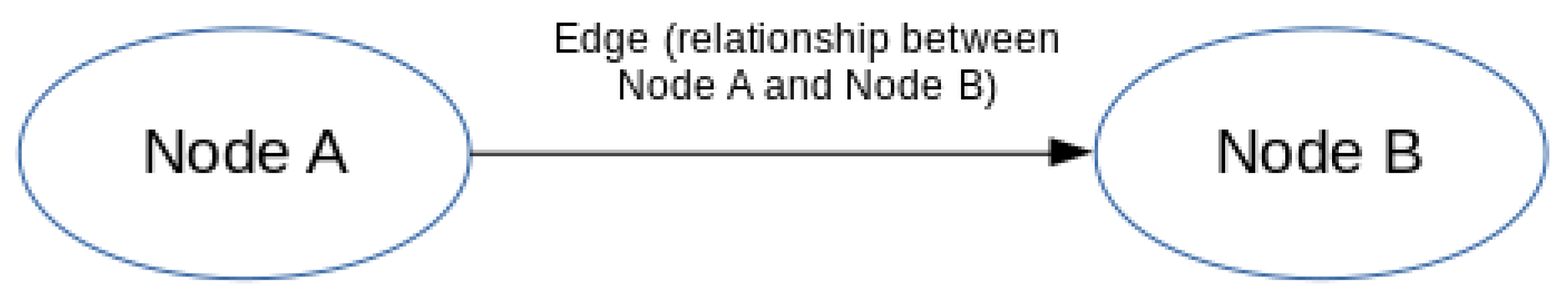
Knowledge Graphs (KG) are inspired in interlinking data, modeling unstructured information in a meaningful way. A KG is also known as a Knowledge Base (technology that stores complex unstructured or structured information/data), and it is defined as a network in which the nodes indicate entities and the edges indicate their relation. DBpedia (http://aksw.org/Projects/DBpedia.html accessed on 7 May 2021), YAGO (https://yago-knowledge.org/ accessed on 7 May 2021), and SUMO (http://www.adampease.org/OP/index.html accessed on 8 May 2021) are three examples of huge KG that have been released on the past decade, since they have become an outstanding resource for NLP applications, such as Question-Answering (QA) [58,59]. Formally, the essence of KG is triples, and its general form is explained in Definition 1.
Definition 1.
Knowledge Graph (KG) A knowledge graph, denoted as KG, is a triple , where is a set of entities, represents a set of binary relations, and represents the relationships between entities (fact triple set).
Since the KG stores real-world information in RDF-style triplets (http://www.w3.org/TR/rdf11-concepts/ accessed on 8 July 2021), such as , it can be employed to support the representation of knowledge in different applications. For example, in the medical industry, it can provide a clear visual representation of diseases as mentioned in [23]; in e-commerce, it maps clients’ purchase intentions with sets of candidate products as mentioned in [60]. The construction of KG is based on its entities (also known as nodes) and their interrelation with other objects, organized in the form of a graph. Each entity is able to share its knowledge with other entities.
In Figure 1, two nodes represent different entities. There is a connection between these two nodes that represents their relationship. The first node (Node A) is known as the subject, the second node (Node B) is known as the object, and their relationship is known as the predicate. This representation is the minimal KG that can exist. It is also known as a semantic triple (codification of a statement in a set of three entities). Figure 2 shows an example of a KG representing the following triples: (“Da Vinci”, “is a”, “Person”), (“Da Vinci”, “painted”, “Mona Lisa”), (“Mona Lisa”, “is located in”, “Louvre”).
3.2. Long-Short-Term Memory (LSTM)
The motivation for using neural networks in this work, in particular LSTM, is due to its proven efficiency in Sentiment Analysis. Although RNNs have proved to be successful in several tasks, it is well-known that it suffers from a significant drawback, namely the vanishing-gradient problem [61], making it difficult for the network to learn long-distance dependencies. The use of memory units in the network helps to overcome this drawback. These memory units decide what the network should remember and what it should forget. These units are part of the LSTM networks.
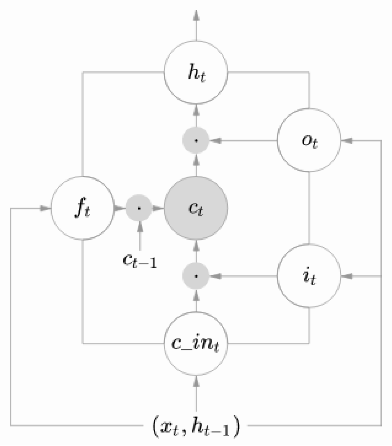
The most important concept of LSTM is the cell state. The cell state is the mechanism to transfer information throughout the network [62], the cell state is the memory of the network, which allows it to remember or forget information. This information is added or removed by three gates, namely the input, output, and forget gates, defined by Equations (1)–(3), respectively. These gates use a activation function (represented by g) [63,64]. Below are the equations that represent the gates. Upper-case variables represent matrices, while lower-case variables represent vectors. The matrices and contain the weights of the recurrent connections and the input, q index could be either the input gate (i), the output gate (o) or the forget gate (f):
- The input gate (which tells what new information will be stored in a cell) is defined as:
- The output gate (which provides the activation function with the final output of the LSTM block at a timestamp t) is defined as:
- The forget gate (which tells what information should be forgotten) is defined as:
The initial values are and . The variables are:
- : represents a vector of dimension d to the LSTM unit.
- : activation vector of the forget gates.
- : activation vector of input gates.
This mechanism is represented in Figure 3. The cell can keep a piece of information for long-term periods of time and the gradient descent is not affected, and this makes it possible to learn long dependencies on phrases. This is the main reason for choosing LSTM networks. This network can be trained in a supervised environment mixed with back-propagation algorithms.
For the case of Bi-LSTM, it applies the same mechanism as in LSTM, but in this network the input is fed through the neural network from the beginning to the end and then again from the end to the beginning; this bi-directionality is what gives it the name Bi-LSTM. It is expected that this neural network learns faster than LSTM.
4. Sentiment Analysis Based on KG: The Proposal
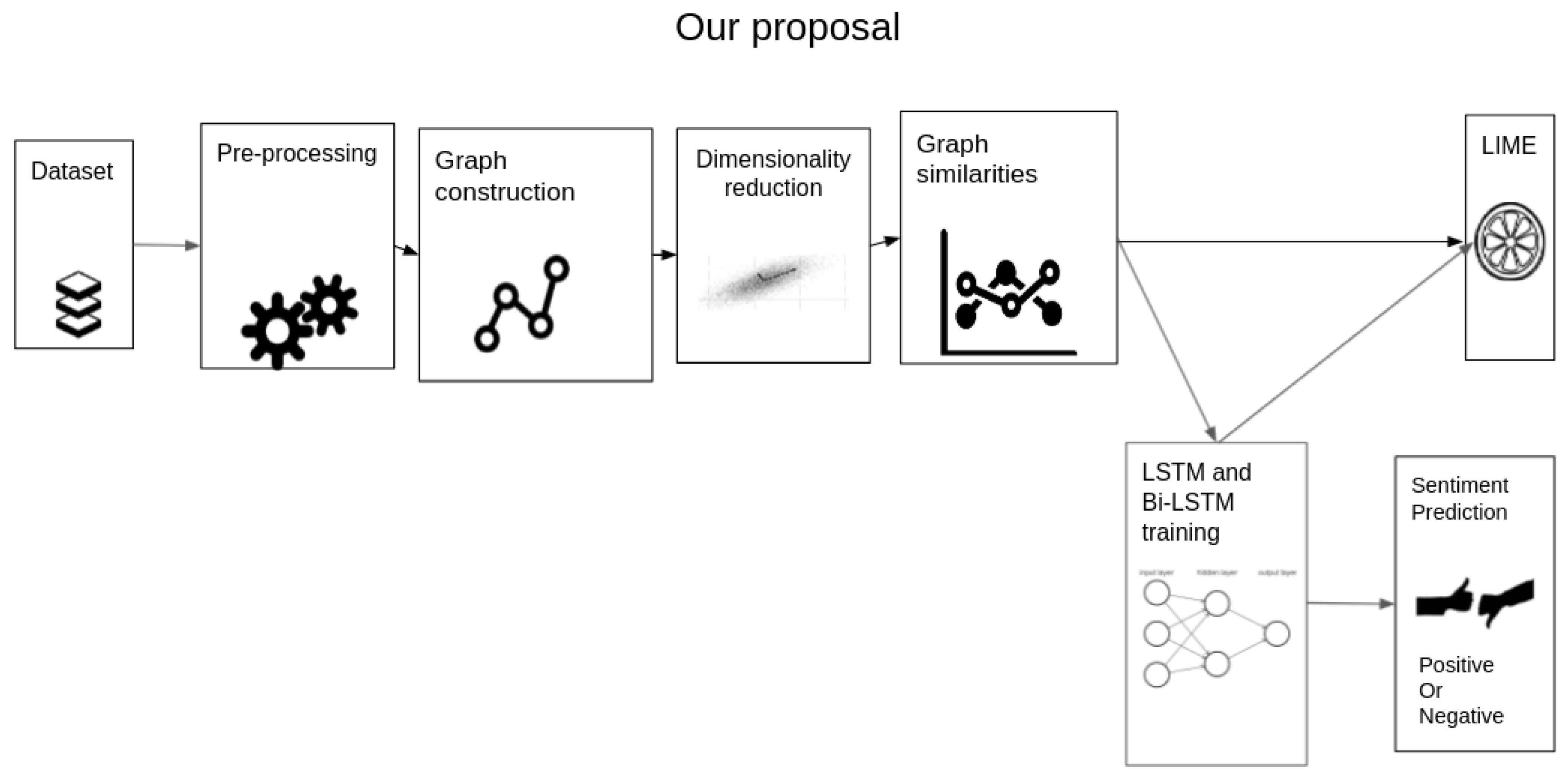
The proposed method is inspired by other works that are related to the representation of text as graphs [52]. The combination of Knowledge Graphs and Deep Learning techniques represents a different approach from the traditional n-gram representation with the aim of better understanding of the sentiment, which is related to the representation of text as graphs. KG and vector representation of text lead the Sentiment Analysis task in tweets. Figure 4 illustrates every step taken in the proposal. The details of these steps are explained below.
The proposed approach starts with the construction of a dataset, that could be done in different ways, for example, by querying an API or by accessing a public dataset. In this case, the dataset is well-known and it has been used in previous studies. This dataset should contain text information and a label. Following to the dataset extraction, the data need to be pre-processed; the pre-processing step includes filtering unwanted values in the text, lower-casing it, filtering stop words, etc. Then, the graph construction consists of using KG (see Definition 1) to create the polarity classes for positive and negative sentiment and the representation for the tweets in KG form. Each tweet and the sentiment polarities (positive and negative) are represented as a KG. They are built from a subset of the training set—i.e., one part of the training set is taken to produce the KG representing sentiment polarities (one for positive, one for negative) and the other produces KG for every tweet. Then, the dimensions of these graphs is reduced by applying the mutual information criteria, reducing in this way the number of edges of the graphs. Afterward, the distance metrics between the graphs of the tweets and the polarities are evaluated, to obtain similarity measurements. The similarity comparison between the sentiment polarities and the individual KG produces vectors used to train a classifier model, in this case an LSTM network and a Bi-LSTM network. On the test set, each new tweet to be classified is transformed into a KG and then its similarity to the polarity graphs is measured. Deep Learning models combined with the explicit semantics of texts represented by KG and the similarity metrics facilitate the traceability and explainability of the classification results since these graphs can be visually inspected, while the accuracy of the results is ensured. As an aggregated step, the proposal provides interpretability based on LIME. Once the model is trained, it is important to try to understand how it makes predictions and what features are the most important. The details of these steps are presented in the following sections.
4.1. Dataset
The dataset used for the implementation of the proposed approach is Sentiment140 (http://cs.stanford.edu/people/alecmgo/trainingandtestdata.zip accessed on 2 July 2019), which contains 1,600,000 tweets in English, labeled positive, negative, and neutral, as well as meta-data describing each tweet. For the purposes of Sentiment Analysis, only the content of the tweet text along with its tag is required. However, the neutral tag is not considered in this work; therefore, the tweets considered are the ones that contain sentiment.
The dataset was divided into two pieces, one for training the model and the other for testing it. The first 80% of the dataset was for training and the other 20% for testing. The process of transforming the tweets into small KG also took place for this last 20%, and the measurement of the similarities with the same metrics is explained in Section 4.5. Finally, the predictive model runs with these new similarities as input to compute the score of the model and its efficiency.
4.2. Pre-Processing
The pre-processing of the raw text involves removal of characters that do not help to detect Sentiment, such as HTML characters, elements that contain the special character “@”, URL, and hashtags; transformation to lower case, since the analysis is sensitive to case letters; expansion of English contraction, such as don’t, won’t; elimination of long words; elimination of tweets that contain words longer than 45 characters; elimination of stop words, such as the, a, this. Nonetheless, it does not include the lemmatization, since the interest resides on the inflected form of the words, and not on their normal form.
4.3. Graph Construction
The automatic construction of KG demands finding a way to recognize the entities and their relationships. The following steps describe the KG construction process:
- Sentence segmentation: Split the text (a tweet, in this case) into sentences. Therefore, a sentence has one object and one subject.
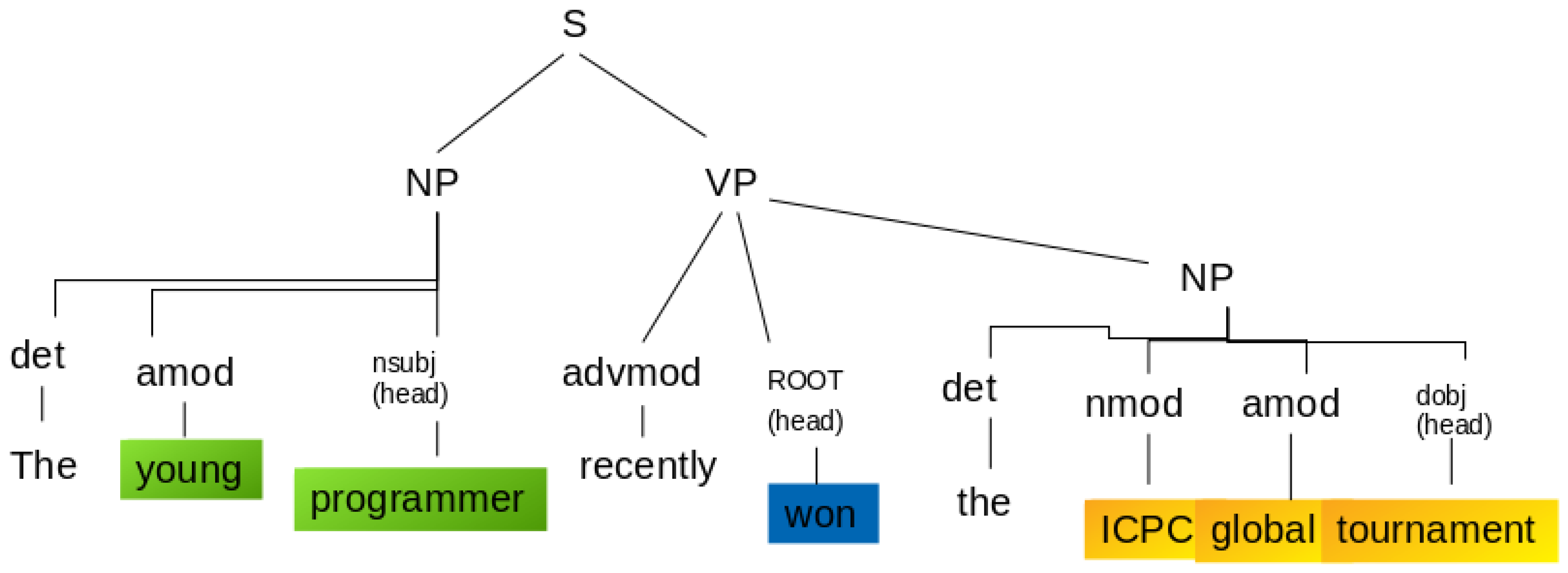
- Entities extraction: An entity is a Noun or a Noun Phrase (NP). sentencePart of Speech (PoS) tags help in this case to extract a single-word entity from a sentence. For example, in the sentence “Rafael won the first prize”, the PoS tags classify “Rafael” as a Nominal Subject (nsubj), and “prize” as a Direct Object (dobj); both of them are syntactic dependency tags that contain the information needed for the formation of the KG entities. For most of the sentences, the use of PoS tags alone is almost enough. Nonetheless, for some sentences, the entities span multiple words; therefore, the syntactic dependency tags are not sufficient. For example, in the sentence “The 42-year-old won the prize”, “old” is classified as the nsubj; nonetheless, “42-year-old” would be preferable to extract instead. The “42-year” is classified as adjectival modifier (amod)—i.e., it is a modifier of “old”. Something similar happens with the dobj. In this case, there are no modifiers but there are compound words (collections of words that form a new term with a different meaning); for example, “ICP global tournament” instead of the word “prize”. The PoS tags only retrieve “tournament” as the dobj; however, the extraction of compound words is critical. These words are “ICP” and “global”. Hence, the subjects and objects along with its punctuation marks, modifiers, and also compound words are essential for the extraction. Therefore, parsing the dependency tree of the sentence contributes to this task. To accomplish this, the modifier of the subject is extracted (amod in the dependency tree).
For example, for the sentence “The young programmer recently won the ICPC global tournament”, its parse tree can give information about the PoS tags, defining the determiners, verbs, modifiers, and subjects and grouping them in verb phrases (VP) and noun phrases (NP) sub-trees, as shown in Figure 5. In this example, the entity “young programmer” is identified as a subject and “ICPC global tournament” as the object of the sentence. Therefore, for these cases, it is needed to include modifiers and adverbs in the entities of the KG.
- 3.
- Relationships extraction: To extract the relations between nodes, it is convenient to assume that it refers to the main verb of the sentence. Therefore, the main verb represents the relationship between two entities. In the sentence in Figure 5, the predicate is “won”, which is also tagged as “ROOT” or main verb.
- 4.
- Building the knowledge graph: In order to build the KG, it is necessary to work with a network in which the nodes are the entities, and the edges between the nodes represent the relations between the entities. It needs to be a directed graph, which means that the relation between two nodes is unidirectional.
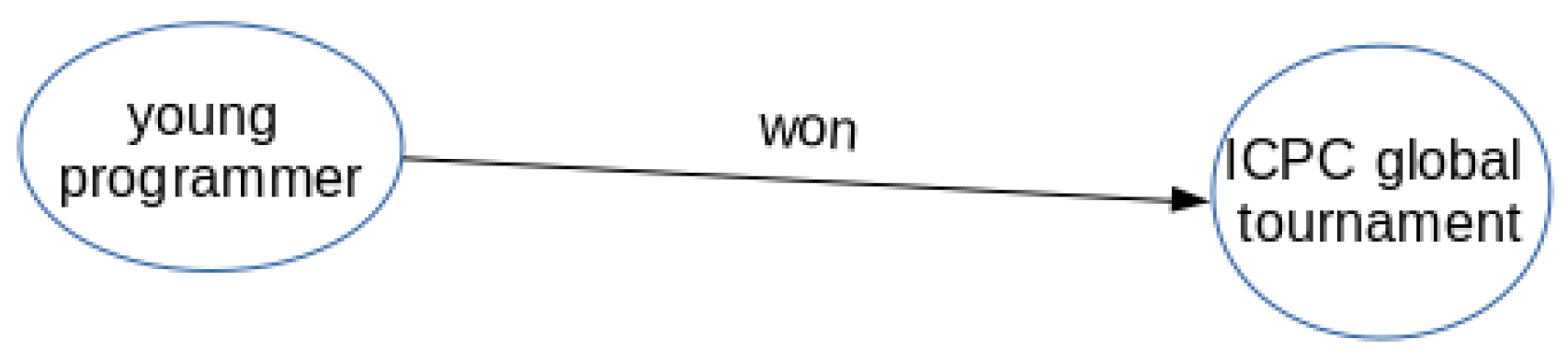
Figure 6 shows a KG representation of the parser tree presented in Figure 5. The entities of this small KG are given by “young programmer” and “ICPC global tournament”, and the relation between the entities is the main verb, in this case the verb “won”. In this way, a sentence is enough for constructing a KG. The two polarity KG are constructed from positive tagged tweet sets and another negative tagged set, respectively, taken from the training dataset. Then, with the other part of the training dataset, a KG is generated for each tweet.
4.4. Dimensionality Reduction
Typical Machine Learning methodologies imply feature selection or dimensionality reduction in order to improve metrics, such as accuracy or the mean squared error [65]. In this work, the mutual information criteria for graphs is used. This criterion is applied after the creation of the KG for the sentiment classes and tweets in the training process. Dimensionality reduction discards edges so the graphs become smaller; therefore, computational resources are optimized.
The edge filter with the containment similarity metric is used. The mutual information criterion between the term (t) (edge) and category (c) (sentiment class) is defined in Equation (4) [66], where A is the number of times that t exists in the graph of sentiment polarities and in the graphs of the tweets of the second part of the training process; B is the number of times that t does not exist in the graph of sentiment polarities but exists in the graphs of the tweets of the second part of the training process; C is the number of times the second part of the training process expresses the sentiment of c and does not contain t; N is the total number of documents in the second part of the training process.
Finally, the average factor, , defines the contribution of the edge to the sentiment graphs. For every edge, Equation (5) computes the global mutual information, where is the percentage of tweets from the second part of the training process that express the sentiment . Naturally, if this contribution for a certain edge is smaller than a certain threshold (chosen accordingly to the problem or criteria of the researcher), then the edge is discard.
Tweets have a limitation in length; thus, they are short pieces of text. Therefore, it is necessary to use a classification model able to deal with this characteristic and also deal with the long dependencies in the words in a tweet (i.e., dependencies of words that are not strictly adjacent words or morphemes). In this sense, this work is based on LSTM and Bi-LSTM networks, that are able to manage these text conditions [67].
4.5. Graph Similarities
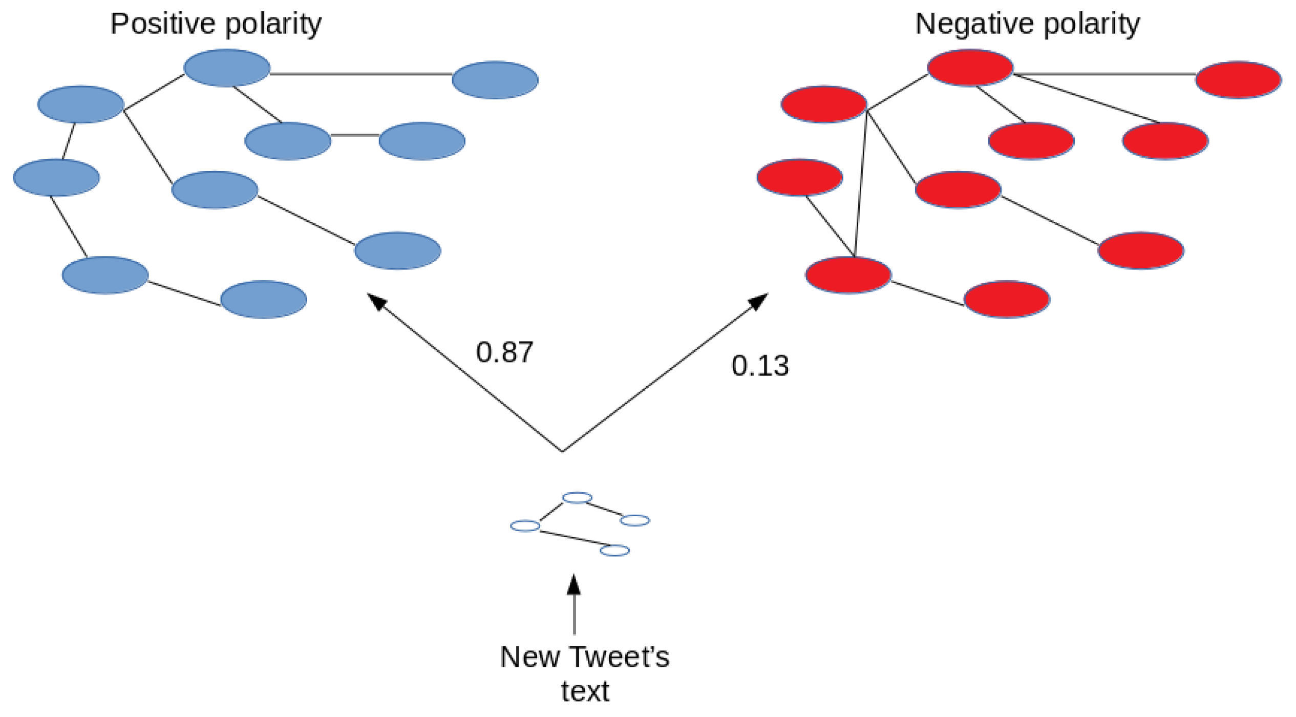
The similarity between the graph that represents the tweet and the polarity graphs expresses how the tweet is related to one polarity or to another. This indicates that if the graph of a tweet is more similar to the positive polarity graph, this tweet is considered as expressing a positive sentiment (as shown in Figure 7). Each similarity distance means the percentage of correlation between the new graph and the polarity graphs. If a tweet is more related to a positive polarity, and therefore its correlation is higher to this polarity, then a positive label is assigned to this tweet. Otherwise, a negative label is assigned.
To calculate the similarity of a tweet KG, the following graph similarity metrics are relevant:
- Containment similarity measurement: This is a graph similarity measurement that expresses the percentage of common edges between the graphs, taking the size of the smaller graph as the factor of this measurement. Given as the knowledge graph of a new document or tweet, and as the knowledge graph of a polarity, Equation (6) calculates the containment similarity measurement between these two graphs, where represents a function that calculates the amount of common edges between the two graphs passed as parameters.
- Maximum common sub-graph similarity measurement: Given two graphs, and , the maximum common sub-graph of them, is a sub-graph of both graphs, such that there is no other sub-graph of and with more nodes [68]. The measurement of maximum common sub-graph is based on the sizes of common sub-graph between the two graphs. Detecting the maximum common sub-graph between two graphs with labeled nodes is a linear problem. Equation (7) is used to calculate the maximum common sub-graph between and , where MCSN is a function that returns the number of nodes that are contained in the maximum common sub-graph of these graphs.
- Maximum common sub-graph number of edges: It takes into account the number of common edges that are contained in the maximum common sub-graph instead of the nodes in common. This is reflected in Equation (8), where the Maximum Common Subgraph of Edges (MCSE) is the number of edges contained in the maximum common sub-graph.
The is defined as the quantity of edges contained in the maximum common sub-graph and maintain the same direction in both and . It is also possible to measure the similarity using the edges but not taking into account if the direction is maintained; this is measured in Equation (9), where represents the Maximum Common Subgraph of Undirected Edges (i.e., total number of edges contained in the maximum common sub-graph regardless of their direction).
Thus, the vector used to train a classifier have eight similarity metrics (four for each polarity), and it has the following format:
The motivation of using these metrics is that they offer a numerical representation of the graphs and also reduce the data structure repetitions [69].
4.6. LSTM and Bi-LSTM
As a predictive model, there is an implementation of two neural networks, an LSTM and a Bi-LSTM. These models take as input the vector constructed in the previous step (see Section 4.5). These networks are considered as the most effective models for sentiment prediction, since they have demonstrated their value in the task of recognizing sentiment [70].
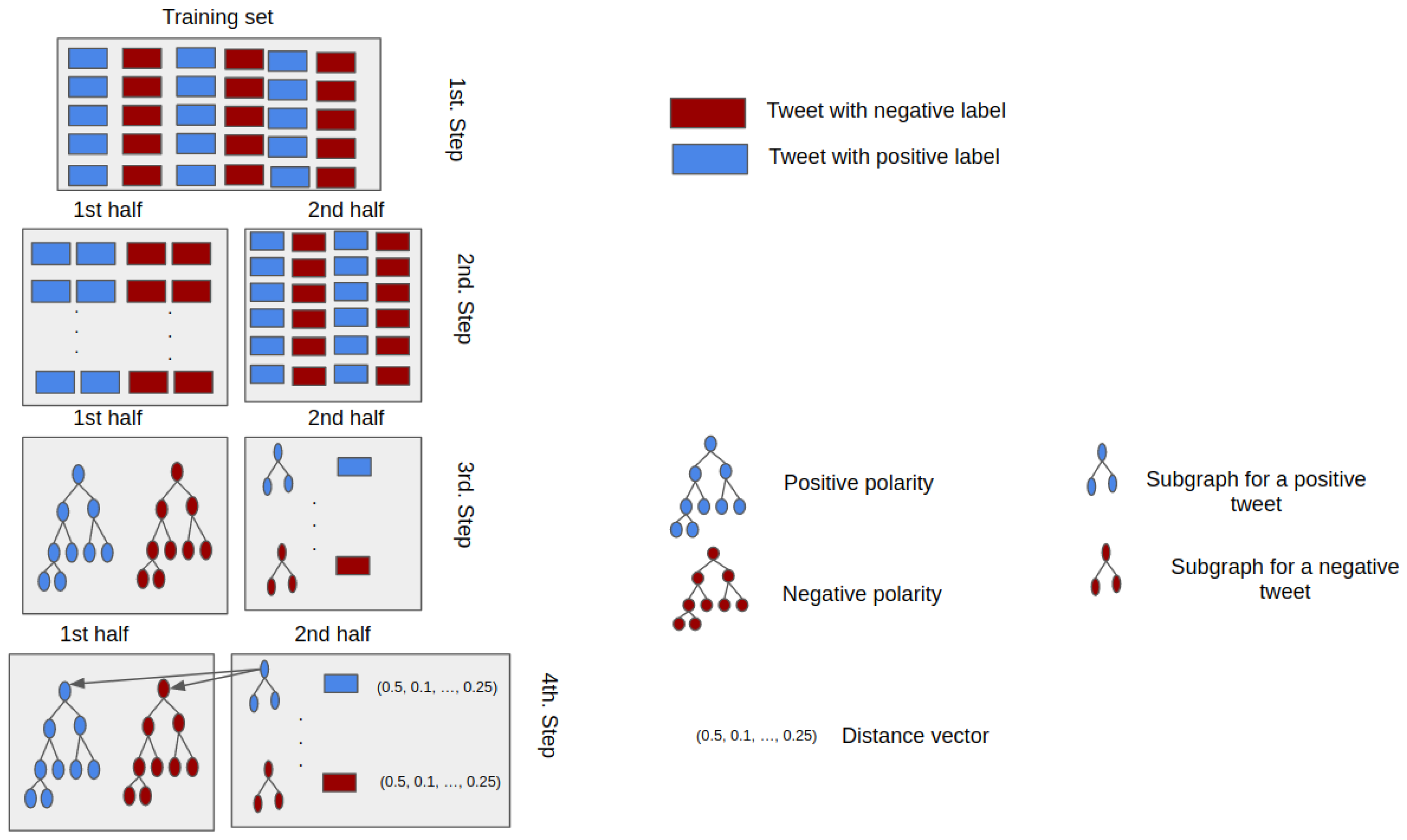
Figure 8 illustrates the steps for the construction of the training set and the respective KG. The definition of the training set (a percentage of the whole dataset) occurs first (first step). The second step is divided into two parts. The first part is used to build the KG that represents the sentiment classes (positive and the negative polarities); labeled tweets (positive and negative sentiment) enables the creation of a positive and negative polarity KG (3rd step). The second part, in the third step, represents the creation of a KG for every tweet, following the process explained in Section 4.3. Finally, the similarity metric between every KG representing the tweet with the KG of positive and negative polarities is calculated, resulting in a vector of eight dimensions (four measurements against the positive KG and four against the negative KG—see Section 4.5) and a label of a sentiment (4th step).
Naturally, the creation of a test set follows the same steps as previously described. The classifier’s input vectors contain the eight different similarity measurements.
The 10-fold cross validation approach is part of the training of the LSTM and Bi-LSTM classifiers, using the same training data. In every fold, 90% of the tweets are used for training and 10% for testing. No added data were used, and no other statistical measurements were taken.
After the model is trained, it is able to execute predictions on the test set. The test set was created with the same rules as the training set; this test set is useful for measuring the performance of the model.
4.7. Lime-Based Interpretability
Once the model is trained, the results are passed to LIME to be interpreted. LIME explains the behavior of the classifier around the predicted instance; it perturbs the input, changing it into its neighbors and sees how the model behaves. Then, LIME weights the perturbed data points and compares them with the original sample. It weights these perturbed data points by their similarity with the original sample and learns an interpretable model on these weights and the associated prediction. For example, to explain the prediction of the sentiment “I love this summer”, LIME perturbs the sentence and makes predictions for sentences like “I love summer”, “I love”, “I summer”, which are examples of perturbation of the original sentence/sample. The classifier is expected to learn that the word “love” is relevant and it expresses the correct sentiment. Thus, after the model is trained and tested, the introduction of interpretability allows us to understand how the predictions were made and the importance of the distance metrics for the KG.
5. Results
This section contains the evaluation of the proposed LSTM and Bi-LSTM enhanced with KG models through the metrics F1-score, precision, and recall and its comparison with state-of-the-art techniques. Afterward, the interpretation of the results and also how the interpretability is done through the use of LIME.
5.1. Performance Evaluation
Implementations of an LSTM (Character n-gram based LSTM) and a Bi-LSTM (Character n-gram based Bi-LSTM) classical versions are implemented as baselines, representing state-of-the-art techniques for learning long-distance dependencies, in order to to evaluate the LSTM enhanced with the KG version (LSTM with KG) and Bi-LSTM enhanced with the KG model (Bi-LSTM with KG). For the traditional character n-gram embeddings versions, the original input is the sentence, and then, using max-pooling, the more important n-grams are extracted, combining the maximum values of each layer of the network in only one vector to finally use a Sigmoid function to make the prediction.
For the implementation, Python 3 with the Keras library and TensorFlow, using GoogleGPUs (https://colab.research.google.com/notebooks/intro.ipynb#recent=true accessed on 3 September 2021), were confirmed to be an extraordinary toolset. GoogleGPUs is a free cloud-based version of a Jupyter notebook, which allows optimizations for big arrays in Colab Notebooks. The hardware available in these notebooks is a 12GB NVIDIA Tesla K80 GPU that can be used up to 12 h continuously. The hyperparameters for optimizations were chosen empirically: (i) Batch size is 500, Max length of the input sequence is 280, since 280 is the maximum length of a tweet, and the embedding matrix is initialized to 0; (ii) Embedding layer created within the Sequential model given by Keras; (iii) SpatialDropout1D layer to delete 1D feature maps, promoting independence between features; and (iv) LSTM and Bi-LSTM layer given by Keras.
These experiments show that Dimensionality Reduction helps to improve the precision of the method, since it decreases the number of edges in the KG. Results are shown in Table 3 in terms of score, precision, and recall.
The proposed approach based on KG has a higher score with LSTM (LSTM with KG in Table 3) than with Bi-LSTM (BI-LSTM with KG in Table 3); nonetheless, this is a more complex and fast convergence model. Comparing both versions of the proposed models with KG against the two classical Deep Learning models, note that the character n-gram-based Bi-LSTM model presents the worst results. LSTM shows better results for both KG and character n-gram-based LSTM. For both cases, scores are quite similar, as results of LSTM with KG are better than results of character n-gram-based LSTM; actually, precision and recall values of LSTM with KG are the best among the four models, meaning that the proposed model is able to make correct predictions and the ratio of correctly predicted values tends to be high as well. These results show that the combination of KG with a classifier is appropriate for detecting the feelings expressed in short texts.
Besides the fact that results are the state of the art for Sentiment Analysis, there are several advantages of the proposed approach: (i) it enables easily creating a KG that can be inspected, which is conducive to more traceable and interpretable classification results; (ii) the explicit semantics of texts are represented by KG, which capture grammar, long-distance dependencies, and neologism and thus are more suitable for detecting sentiment in micro-blogging texts; and (iii) this approach represents a way of doing Sentiment Analysis that can be used in other contexts, for example, recognizing topics based on the semantic provided by KG and expanded with the use of Linked-Data, which are indeed complex KG.
5.2. Interpretability
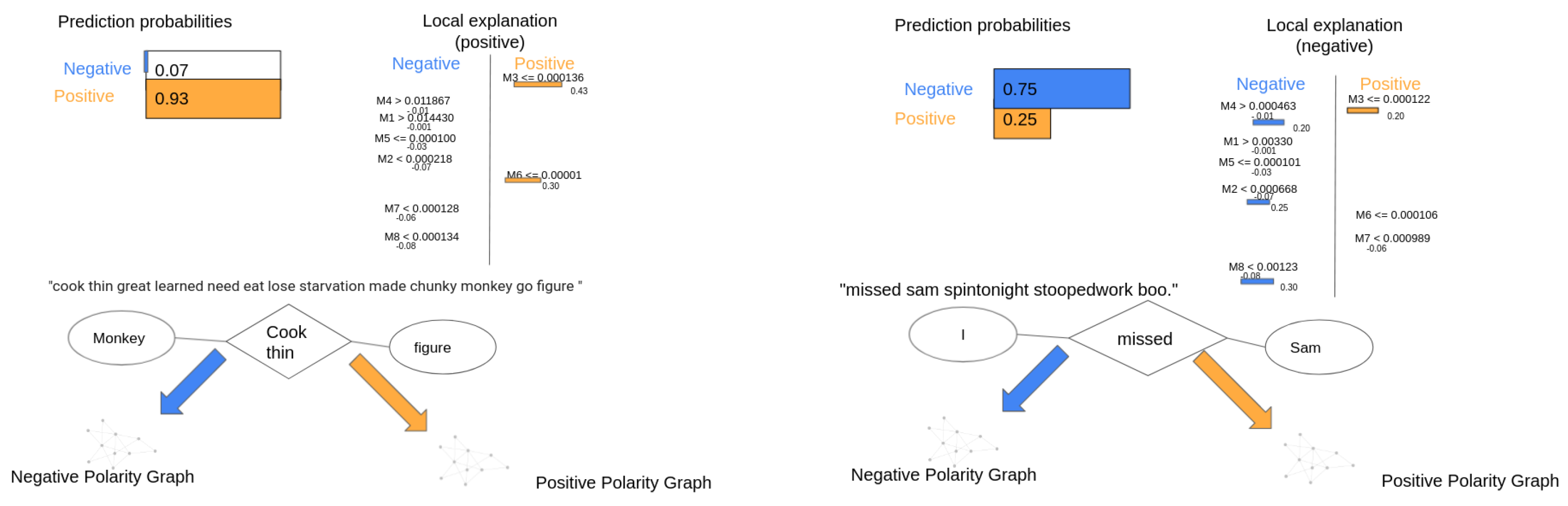
This section illustrates the interpretability of two tweets, one positive and one negative. Figure 9 shows the process of interpretability for a positive (left side) and a negative (right side) tweet. with represents the vector with graph similarity metrics as explained on Section 4.5. The original positive tweet is: “cook thinneed to eat it go figure” and the original negative tweet is: “missed sam spintonight stooped work boo”. After the cleaning process, the first tweet becomes into “cook thin need to eat it go figure”; the similarity metrics vector of this tweet is given by the following values:
It seems obvious that the similarity to the positive class is greater than to the negative class, since the first four similarity measurements show a greater similarity to the positive polarity. The LIME output of this tweet shows that the model is 93% confident that this is a positive classification, because the values of () and () increase the tweet’s chance of being classified as good. In other words, the explanation assigns positive weight to the containment similarity measurement between the Positive Polarity Graph and the KG of the tweet. It also assigns positive weight to the Maximum Common Subgraph of Undirected Edges between these two graphs, i.e., and .
After the cleaning process, the second tweet becomes “missed sam spin tonight stooped work boo”. The graph similarity metrics vector is given by the following values:
The analysis of these similarity metrics is analogous to the previous one. The similarity to the negative class is bigger than to the positive class; therefore, it is considered or classified as negative. The LIME output of this tweet shows that the model is 75% confident that this is a negative classification, because the values of (), (), (), and () increase the chance of the tweet being classified as negative, while the () is the only one that decreases it.
6. Conclusions
This work shows that Knowledge Graphs combined with Deep Learning techniques are able to detect sentiment in short segments of text. Knowledge Graphs can capture structural information of a tweet and also part of its meaning. The proposed model is based on the use of graph techniques and similarity metrics between graphs. The result of the comparison of graphs (i.e., graph similarity measurements) is a vector, which is fed later to the neural networks, which recognize the polarity of the sentiment. The study of sentiment through Knowledge Graphs and Deep Learning represents an interesting challenge that has some limitations. There could be scenarios where the data are limited (small dataset), and this can lead to an under-fitting classifier unable to generalize a rule for distinguishing sentiments.
The recognition of entities and their connections is crucial to the proposed approach, the use of PoS tagging allows performing this operation. Results are comparative with the ones encountered on literature for the same problem. The proposed methodology is simple, and the main contribution is to show that the construction and good manipulation of Knowledge Graphs leads to state-of-the-art results. Knowledge Graphs are suitable for detecting sentiment in micro-blogging texts, provides more informed and traceable Deep Learning algorithms that produce higher accuracy scores, and have the potential to be expanded with the use of Linked-Data, thanks to the properties of the Knowledge Graphs. Adding interpretability with LIME enables a better understanding of the importance of similarity metrics between graphs and gives a deeper insight into what the algorithm is doing, since it focuses on how the prediction is made.
The use of Knowledge Graphs has proven to be useful to detect semantic information; therefore, this type of graph can be applied in other areas. As future work, it is planned to investigate how the Knowledge Graphs interact with other applications, such as cross-domain polarity classification [71], since they use semantic networks and these can be enhanced with the use of Knowledge Graphs. Another future work for the Knowledge Graphs for Sentiment Analysis is in the area of irony detection [72], where the sentiment helps to differentiate between an ironic and non-ironic tweet.
Author Contributions
Conceptualisation: F.A.L., Y.C.C. and M.N.H.; data curation: F.A.L.; methodology: F.A.L., Y.C.C. and M.N.H.; software: F.A.L.; validation, F.A.L., Y.C.C. and M.N.H.; investigation: F.A.L., Y.C.C.; writing—original draft preparation: F.A.L.; Y.C.C.; writing—review and editing: F.A.L., Y.C.C. and M.N.H. All authors have read and agreed to the published version of the manuscript.
Funding
This research received no external funding.
Conflicts of Interest
The authors declare no conflict of interest.
References
- Mostafa, M.M. More than Words: Social Networks’ Text Mining for Consumer Brand Sentiments. Expert Syst. Appl. 2013, 40, 4241–4251. [Google Scholar] [CrossRef]
- Cambria, E.; Das, D.; Bandyopadhyay, S.; Feraco, A. Affective computing and sentiment analysis. In A Practical Guide to Sentiment Analysis; Springer: Cham, Switzerland, 2017; Volume 31, pp. 102–107. [Google Scholar]
- De Albornoz, J.C.; Plaza, L.; Gervás, P.; Díaz, A. A joint model of feature mining and sentiment analysis for product review rating. In European Conference On Information Retrieval; Springer: Berlin/Heidelberg, Germany, 2011; pp. 55–66. [Google Scholar]
- Mirtalaie, M.A.; Hussain, O.K.; Chang, E.; Hussain, F.K. Sentiment analysis of specific product’s features using product tree for application in new product development. In Proceedings of the International Conference on Intelligent Networking and Collaborative Systems, Vancouver, BC, Canada, 24–28 September 2017; pp. 82–95. [Google Scholar]
- Chu, E.; Roy, D. Audio-visual sentiment analysis for learning emotional arcs in movies. In Proceedings of the IEEE International Conference on Data Mining (ICDM), New Orleans, LA, USA, 18–21 November 2017; pp. 829–834. [Google Scholar]
- Oliveira, D.J.S.; Bermejo, P.H.d.S.; dos Santos, P.A. Can social media reveal the preferences of voters? A comparison between sentiment analysis and traditional opinion polls. J. Inf. Technol. Politics 2017, 14, 34–45. [Google Scholar] [CrossRef]
- Agarwal, A.; Xie, B.; Vovsha, I.; Rambow, O.; Passonneau, R.J. Sentiment analysis of twitter data. In Proceedings of the Workshop on Language in Social Media, Portland, OR, USA, 23 June 2011; pp. 30–38. [Google Scholar]
- Rosenthal, S.; Farra, N.; Nakov, P. SemEval-2017 task 4: Sentiment analysis in Twitter. In Proceedings of the 11th International Workshop on Semantic Evaluation, Vancouver, BC, Canada, 3–4 August 2017; pp. 502–518. [Google Scholar]
- Pagolu, V.S.; Reddy, K.N.; Panda, G.; Majhi, B. Sentiment analysis of Twitter data for predicting stock market movements. In Proceedings of the International Conference on Signal Processing, Communication, Power and Embedded System, Odisha, India, 3–5 October 2016; pp. 1345–1350. [Google Scholar]
- Sadegh, M.; Ibrahim, R.; Othman, Z.A. Opinion mining and sentiment analysis: A survey. Int. J. Comput. Technol. 2012, 2, 171–178. [Google Scholar]
- Medhat, W.; Hassan, A.; Korashy, H. Sentiment analysis algorithms and applications: A survey. Ain Shams Eng. J. 2014, 5, 1093–1113. [Google Scholar] [CrossRef] [Green Version]
- Kharde, V.; Sonawane, P. Sentiment analysis of twitter data: A survey of techniques. arXiv 2016, arXiv:1601.06971. [Google Scholar]
- Hussein, D.M.E.D.M. A survey on sentiment analysis challenges. J. King Saud Univ.-Eng. Sci. 2018, 30, 330–338. [Google Scholar] [CrossRef]
- Jianqiang, Z.; Xiaolin, G.; Xuejun, Z. Deep convolution neural networks for twitter sentiment analysis. IEEE Access 2018, 6, 23253–23260. [Google Scholar] [CrossRef]
- Sánchez-Rada, J.F.; Torres, M.; Iglesias, C.A.; Maestre, R.; Peinado, E. A Linked Data Approach to Sentiment and Emotion Analysis of Twitter in the Financial Domain. In Proceedings of the European Semantic Web Conference, Crete, Greece, 25–29 May 2014. [Google Scholar]
- Roshani, S.; Jamshidi, M.B.; Mohebi, F.; Roshani, S. Design and Modeling of a Compact Power Divider with Squared Resonators Using Artificial Intelligence. Wirel. Pers. Commun. 2021, 117, 2085–2096. [Google Scholar] [CrossRef]
- Nazemi, B.; Rafiean, M. Forecasting house prices in Iran using GMDH. Int. J. Hous. Mark. Anal. 2020, 14, 555–568. [Google Scholar] [CrossRef]
- Roshani, M.; Sattari, M.A.; Ali, P.J.M.; Roshani, G.H.; Nazemi, B.; Corniani, E.; Nazemi, E. Application of GMDH neural network technique to improve measuring precision of a simplified photon attenuation based two-phase flowmeter. Flow Meas. Instrum. 2020, 75, 101804. [Google Scholar] [CrossRef]
- Reddy, S.; Allan, S.; Coghlan, S.; Cooper, P. A governance model for the application of AI in health care. J. Am. Med Informatics Assoc. 2020, 27, 491–497. [Google Scholar] [CrossRef] [PubMed]
- Ma, L.; Cheng, S.; Shi, Y. Enhancing Learning Efficiency of Brain Storm Optimization via Orthogonal Learning Design. IEEE Trans. Syst. Man, Cybern. Syst. 2020, 51, 6723–6742. [Google Scholar] [CrossRef]
- Ma, L.; Huang, M.; Yang, S.; Wang, R.; Wang, X. An Adaptive Localized Decision Variable Analysis Approach to Large-Scale Multiobjective and Many-Objective Optimization. IEEE Trans. Cybern. 2021, 1–13. [Google Scholar] [CrossRef]
- Taboada, M. Sentiment Analysis: An Overview from Linguistics. Annu. Rev. Linguist. 2016, 2, 325–347. [Google Scholar]
- Rotmensch, M.; Halpern, Y.; Tlimat, A.; Horng, S.; Sontag, D. Learning a health knowledge graph from electronic medical records. Sci. Rep. 2017, 7, 5994. [Google Scholar] [CrossRef] [PubMed]
- Wang, X.; He, X.; Cao, Y.; Liu, M.; Chua, T.S. Knowledge graph attention network for recommendation. In Proceedings of the 5th International Conference Association for Computing Machinery’s Special Interest Group on Knowledge Discovery and Data Mining, Anchorage, AK, USA, 4–8 August 2019; pp. 950–958. [Google Scholar]
- Zou, X. A survey on application of knowledge graph. J. Phys. Conf. Ser. 2020, 1487, 012016. [Google Scholar] [CrossRef]
- Richardson, A.; Rosenfeld, A. A survey of interpretability and explainability in human-agent systems. In Proceedings of the eXplainable Artificial Intelligence Workshop, Stockholm, Sweden, 13–19 July 2018; pp. 137–143. [Google Scholar]
- Marcinkevičs, R.; Vogt, J.E. Interpretability and explainability: A machine learning zoo mini-tour. arXiv 2020, arXiv:2012.01805. [Google Scholar]
- Mahajan, A.; Shah, D.; Jafar, G. Explainable AI Approach Towards Toxic Comment Classification. In Emerging Technologies in Data Mining and Information Security; Hassanien, A.E., Bhattacharyya, S., Chakrabati, S., Bhattacharya, A., Dutta, S., Eds.; Springer: Singapore, 2021; pp. 849–858. [Google Scholar]
- Magesh, P.R.; Myloth, R.D.; Tom, R.J. An explainable machine learning model for early detection of Parkinson’s disease using LIME on DaTSCAN imagery. Comput. Biol. Med. 2020, 126, 104041. [Google Scholar] [CrossRef]
- Du, M.; Liu, N.; Hu, X. Techniques for interpretable machine learning. Commun. Assoc. Comput. Mach. 2019, 63, 68–77. [Google Scholar] [CrossRef] [Green Version]
- Monga, V.; Li, Y.; Eldar, Y.C. Algorithm unrolling: Interpretable, efficient deep learning for signal and image processing. IEEE Signal Process. Mag. 2021, 38, 18–44. [Google Scholar] [CrossRef]
- Lovera, F.A.; Cardinale, Y.; Buscaldi, D.; Charnois, T.; Homsi, M.N. Deep Learning Enhanced with Graph Knowledge for Sentiment Analysis. In Proceedings of the 6th International Workshop on Explainable Sentiment Mining and Emotion Detection (X-SENTIMENT), Hersonissos, Greece, 7 June 2021. [Google Scholar]
- Ribeiro, M.T.; Singh, S.; Guestrin, C. “Why should i trust you?” Explaining the predictions of any classifier. In Proceedings of the 2016 Conference of the North American Chapter of the Association for Computational Linguistics: Demonstrations, San Diego, CA, USA, 12–17 June 2016; pp. 1135–1144. [Google Scholar]
- Beigi, G.; Hu, X.; Maciejewski, R.; Liu, H. An overview of sentiment analysis in social media and its applications in disaster relief. In Sentiment Analysis and Ontology Engineering; Springer: Cham, Switzerland, 2016; pp. 313–340. [Google Scholar]
- Cieliebak, M.; Dürr, O.; Uzdilli, F. Potential and Limitations of Commercial Sentiment Detection Tools. In Proceedings of the International Conference of the Italian Association for Artificial Intelligence AI* IA, Turin, Italy, 4–6 December 2013; pp. 47–58. [Google Scholar]
- Pang, B.; Lee, L. Opinion mining and sentiment analysis. Found. Trends Inf. Retr. 2008, 2, 1–135. [Google Scholar] [CrossRef] [Green Version]
- Uijlings, J.R.; Smeulders, A.W.; Scha, R.J. Real-time bag of words, approximately. In Proceedings of the Association for Computing Machinery international Conference on Image and Video Retrieval, Kos, Greece, 28 August–2 September 2017; pp. 1–8. [Google Scholar]
- Li, T.; Mei, T.; Kweon, I.S.; Hua, X.S. Contextual bag-of-words for visual categorization. IEEE Trans. Circuits Syst. Video Technol. 2010, 21, 381–392. [Google Scholar] [CrossRef]
- Filliat, D. A visual bag of words method for interactive qualitative localization and mapping. In Proceedings of the IEEE International Conference on Robotics and Automation, Rome, Italy, 10–14 April 2007; pp. 3921–3926. [Google Scholar]
- Sikka, K.; Wu, T.; Susskind, J.; Bartlett, M. Exploring bag of words architectures in the facial expression domain. In Proceedings of the European Conference on Computer Vision, Florence, Italy, 7–13 October 2012; pp. 250–259. [Google Scholar]
- Bekkerman, R.; Allan, J. Using Bigrams in Text Categorization; Technical Report, Technical Report IR-408; Center of Intelligent Information Retrieval, UMass: Amherst, MA, USA, 2004. [Google Scholar]
- Krapac, J.; Verbeek, J.; Jurie, F. Modeling spatial layout with fisher vectors for image categorization. In Proceedings of the International Conference on Computer Vision, Barcelona, Spain, 6–13 November 2011; pp. 1487–1494. [Google Scholar]
- Wang, X.; McCallum, A.; Wei, X. Topical n-grams: Phrase and topic discovery, with an application to information retrieval. In Proceedings of the Seventh IEEE International Conference on Data Mining (ICDM), Omaha, Nebraska, 28–31 October 2007; pp. 697–702. [Google Scholar]
- Severyn, A.; Moschitti, A. Twitter sentiment analysis with deep convolutional neural networks. In Proceedings of the 38th International ACM SIGIR Conference on Research and Development in Information Retrieval, Santiago, Chile, 9–13 August 2015; pp. 959–962. [Google Scholar]
- Yanmei, L.; Yuda, C. Research on Chinese micro-blog sentiment analysis based on deep learning. In Proceedings of the 8th International Symposium on Computational Intelligence and Design (ISCID), Hangzhou, China, 12–13 December 2015; pp. 358–361. [Google Scholar]
- Arras, L.; Montavon, G.; Müller, K.R.; Samek, W. Explaining recurrent neural network predictions in sentiment analysis. arXiv 2017, arXiv:1706.07206. [Google Scholar]
- Yanagimoto, H.; Shimada, M.; Yoshimura, A. Document similarity estimation for sentiment analysis using neural network. In Proceedings of the 12th International Conference on Computer and Information Science, Niigata, Japan, 16–20 June 2013; pp. 105–110. [Google Scholar]
- Li, C.; Xu, B.; Wu, G.; He, S.; Tian, G.; Hao, H. Recursive deep learning for sentiment analysis over social data. In Proceedings of the International Joint Conferences on Web Intelligence and Intelligent Agent Technologies, Warsaw, Poland, 11–14 August 2014; pp. 180–185. [Google Scholar]
- Basiri, M.E.; Nemati, S.; Abdar, M.; Cambria, E.; Acharya, U.R. ABCDM: An attention-based bidirectional CNN-RNN deep model for sentiment analysis. Future Gener. Comput. Syst. 2021, 115, 279–294. [Google Scholar] [CrossRef]
- Silhavy, R.; Senkerik, R.; Oplatkova, Z.K.; Silhavy, P.; Prokopova, Z. Artificial intelligence perspectives in intelligent systems. In The 5th Computer Science Online Conference; Springer: Cham, Switzerland, 2016; pp. 249–261. [Google Scholar]
- Castillo, E.; Cervantes, O.; Vilarino, D.; Báez, D.; Sánchez, A. UDLAP: Sentiment analysis using a graph-based representation. In Proceedings of the 9th International Workshop on Semantic Evaluation, Denver, Colorado, 4–5 June 2015; pp. 556–560. [Google Scholar]
- Violos, J.; Tserpes, K.; Psomakelis, E.; Psychas, K.; Varvarigou, T. Sentiment analysis using word-graphs. In Proceedings of the 6th International Conference on Web Intelligence, Mining and Semantics, Nîmes, France, 13–15 June 2016; pp. 1–9. [Google Scholar]
- Bijari, K.; Zare, H.; Kebriaei, E.; Veisi, H. Leveraging deep graph-based text representation for sentiment polarity applications. Expert Syst. Appl. 2020, 144, 113090. [Google Scholar] [CrossRef] [Green Version]
- Vizcarra, J.; Kozaki, K.; Ruiz, M.T.; Quintero, R. Knowledge-based sentiment analysis and visualization on social networks. New Gener. Comput. 2021, 39, 199–229. [Google Scholar] [CrossRef]
- Díaz-Rodríguez, N.; Lamas, A.; Sanchez, J.; Franchi, G.; Donadello, I.; Tabik, S.; Filliat, D.; Cruz, P.; Montes, R.; Herrera, F. EXplainable Neural-Symbolic Learning (X-NeSyL) methodology to fusedeep learning representations with expert knowledge graphs: The MonuMAI cultural heritage use case. arXiv 2021, arXiv:2104.11914. [Google Scholar]
- Dieber, J.; Kirrane, S. Why model why? Assessing the strengths and limitations of LIME. arXiv 2020, arXiv:2012.00093. [Google Scholar]
- Sosic, R.; Leskovec, J. Large scale network analytics with SNAP: Tutorial at the World Wide Web 2015 Conference. In Proceedings of the 24th International Conference on World Wide Web, Florence, Italy, 18–22 May 2015; pp. 1537–1538. [Google Scholar]
- Huang, X.; Zhang, J.; Li, D.; Li, P. Knowledge graph embedding based question answering. In Proceedings of the Twelfth Association for Computing Machinery International Conference on Web Search and Data Mining, Melbourne, VIC, Australia, 11–15 February 2019; pp. 105–113. [Google Scholar]
- Zhang, Y.; Dai, H.; Kozareva, Z.; Smola, A.J.; Song, L. Variational reasoning for question answering with knowledge graph. In Proceedings of the Thirty-Second Association for the Advancement of Artificial Intelligence Conference on Artificial Intelligence, New Orleans, LA, USA, 2–7 February 2018. [Google Scholar]
- Teru, K.; Denis, E.; Hamilton, W. Inductive relation prediction by subgraph reasoning. In Proceedings of the International Conference on Machine Learning, 13–18 July 2020; pp. 9448–9457. [Google Scholar]
- Roodschild, M.; Sardiñas, J.G.; Will, A. A new approach for the vanishing gradient problem on sigmoid activation. Prog. Artif. Intell. 2020, 9, 351–360. [Google Scholar] [CrossRef]
- Huang, F.; Li, X.; Yuan, C.; Zhang, S.; Zhang, J.; Qiao, S. Attention-Emotion-Enhanced Convolutional LSTM for Sentiment Analysis. IEEE Trans. Neural Netw. Learn. Syst. 2021, 1–14. [Google Scholar] [CrossRef]
- Ito, Y. Approximation of continuous functions on Rd by linear combinations of shifted rotations of a sigmoid function with and without scaling. Neural Netw. 1992, 5, 105–115. [Google Scholar] [CrossRef]
- Behera, R.; Jena, M.; Rath, S.; Misra, S. Co-LSTM: Convolutional LSTM model for sentiment analysis in social big data. Inf. Process. Manag. 2021, 58, 102435. [Google Scholar] [CrossRef]
- Chagheri, S.; Calabretto, S.; Roussey, C.; Dumoulin, C. Feature vector construction combining structure and content for document classification. In Proceedings of the 6th International Conference on Sciences of Electronics, Technologies of Information and Telecommunications (SETIT), Sousse, Tunisia, 21–24 March 2012; pp. 946–950. [Google Scholar]
- Xu, Y.; Jones, G.J.; Li, J.; Wang, B.; Sun, C. A study on mutual information-based feature selection for text categorization. J. Comput. Inf. Syst. 2007, 3, 1007–1012. [Google Scholar]
- Wang, B.; Liu, W.; Han, G.; He, S. Learning Long-Term Structural Dependencies for Video Salient Object Detection. IEEE Trans. Image Process. 2020, 29, 9017–9031. [Google Scholar] [CrossRef]
- Bunke, H. On a relation between graph edit distance and maximum common subgraph. Pattern Recognit. Lett. 1997, 18, 689–694. [Google Scholar] [CrossRef]
- Quer, S.; Marcelli, A.; Squillero, G. The Maximum Common Subgraph Problem: A Parallel and Multi-Engine Approach. Computation 2020, 8, 48. [Google Scholar] [CrossRef]
- Jin, Z.; Yang, Y.; Liu, Y. Stock closing price prediction based on sentiment analysis and LSTM. Neural Comput. Appl. 2020, 32, 9713–9729. [Google Scholar] [CrossRef]
- Franco-Salvador, M.; Cruz, F.L.; Troyano, J.A.; Rosso, P. Cross-domain polarity classification using a knowledge-enhanced meta-classifier. Knowl.-Based Syst. 2015, 86, 46–56. [Google Scholar] [CrossRef] [Green Version]
- Farías, D.I.H.; Patti, V.; Rosso, P. Irony Detection in Twitter: The Role of Affective Content. Assoc. Comput. Mach. Trans. Internet Technol. 2016, 16, 1–24. [Google Scholar] [CrossRef] [Green Version]
Figure 1.
Basic graph with two entities and its relationship.

Figure 2.
Extended graph with two entities and its relationship.

Figure 3.
LSTM’s cell gates and mechanism.

Figure 4.
Pipeline that represents the proposal’s steps.

Figure 5.
Tree parser representation of the sentence: “The young programmer recently won the ICPC global tournament”.
Figure 5.
Tree parser representation of the sentence: “The young programmer recently won the ICPC global tournament”.

Figure 6.
Knowledge Graph representation of the sentence: “The young programmer recently won the ICPC global tournament”.
Figure 6.
Knowledge Graph representation of the sentence: “The young programmer recently won the ICPC global tournament”.

Figure 7.
Similarity measurements.

Figure 8.
Transformation stages of a dataset to its vector form in the Knowledge Graph Method.

Figure 9.
Local explanation of a positive and negative tweet, on the left and right, respectively.

Table 1.
Deep Learning techniques and results.
| Work | Model | Dataset | Result |
|---|---|---|---|
| Yanagimoto et al., 2013 [47] | DNN | T&C New | F-score of 90.8% of accuracy |
| Li et al., 2014 [48] | RNDM | 2270 movie reviews from websites | Accuracy of 90.8% |
| Severyn and Moschitti, 2015 [44] | CNN | Semeval-2015 | F-measure score sub-task A: 84.19% and sub-task B: 64.69% |
| Yanmei and Yuda, 2015 [45] | CNN | 1000 micro-blog comments | Statistical model with average of 85.4% of accuracy |
| Silhavy et al., 2016 [50] | HBRNN | 150,175 labeled reviews from 1500 hotels | HBRNN outperformed the rest of the methods. |
| Arras et al., 2017 [46] | RNN | 11,855 single sentences from movies review | Accuracy of 82.9% for binary classification (positive and negative). |
| Basiri et al., 2021 | ABCDM | Five review and Twitter datasets | Accuracy up to 92% |
Table 3.
Results for experiments.
| Model | Precision | Recall | |
|---|---|---|---|
| LSTM with KG | 0.884 | 0.880 | 0.890 |
| Bi-LSTM with KG | 0.757 | 0.690 | 0.840 |
| Character n-gram based LSTM | 0.849 | 0.840 | 0.860 |
| Character n-gram based Bi-LSTM | 0.852 | 0.851 | 0.856 |
Publisher’s Note: MDPI stays neutral with regard to jurisdictional claims in published maps and institutional affiliations. |
© 2021 by the authors. Licensee MDPI, Basel, Switzerland. This article is an open access article distributed under the terms and conditions of the Creative Commons Attribution (CC BY) license (https://creativecommons.org/licenses/by/4.0/).
Share and Cite
MDPI and ACS Style
Lovera, F.A.; Cardinale, Y.C.; Homsi, M.N. Sentiment Analysis in Twitter Based on Knowledge Graph and Deep Learning Classification. Electronics 2021, 10, 2739. https://doi.org/10.3390/electronics10222739
AMA Style
Lovera FA, Cardinale YC, Homsi MN. Sentiment Analysis in Twitter Based on Knowledge Graph and Deep Learning Classification. Electronics. 2021; 10(22):2739. https://doi.org/10.3390/electronics10222739
Chicago/Turabian StyleLovera, Fernando Andres, Yudith Coromoto Cardinale, and Masun Nabhan Homsi. 2021. "Sentiment Analysis in Twitter Based on Knowledge Graph and Deep Learning Classification" Electronics 10, no. 22: 2739. https://doi.org/10.3390/electronics10222739
Note that from the first issue of 2016, this journal uses article numbers instead of page numbers. See further details here.