
A Metaheuristic Based Approach for the Customer-Centric Perishable Food Distribution Problem


1
TICLab, ESIN, International University of Rabat, Rabat 11100, Morocco
2
Models of Decision and Optimization Research Group, Department of Computer Science and A.I., Universidad de Granada, 18014 Granada, Spain
3
Modeling and Mathematical Structures Laboratory, Sidi Mohamed Ben Abdellah University, Fez 30050, Morocco
*
Authors to whom correspondence should be addressed.
Electronics 2021, 10(16), 2018; https://doi.org/10.3390/electronics10162018
Submission received: 9 July 2021
/
Revised: 17 August 2021
/
Accepted: 19 August 2021
/
Published: 20 August 2021
(This article belongs to the Special Issue 10th Anniversary of Electronics: Recent Advances in Computer Science & Engineering)
Abstract
:High transportation costs and poor quality of service are common vulnerabilities in various logistics networks, especially in food distribution. Here we propose a many-objective Customer-centric Perishable Food Distribution Problem that focuses on the cost, the quality of the product, and the service level improvement by considering not only time windows but also the customers’ target time and their priority. Recognizing the difficulty of solving such model, we propose a General Variable Neighborhood Search (GVNS) metaheuristic based approach that allows to efficiently solve a subproblem while allowing us to obtain a set of solutions. These solutions are evaluated over some non-optimized criteria and then ranked using an a posteriori approach that requires minimal information about decision maker preferences. The computational results show (a) GVNS achieved same quality solutions as an exact solver (CPLEX) in the subproblem; (b) GVNS can generate a wide number of candidate solutions, and (c) the use of the a posteriori approach makes easy to generate different decision maker profiles which in turn allows to obtain different rankings of the solutions.
1. Introduction
In recent years, the global food market has shown substantial growth; therefore, posing new challenges, including in the global logistics market of perishable foods. It is widely known that the processing of the later is different from the distribution of other goods because they deteriorate continuously and have an expiration date. The transportation process is the most critical phase in the entire food supply chain, where the trip path length have the potential to influence the deterioration rate [1,2].
According to the Food and Agriculture Organization FAO (2018) [3], nearly half of fruits and vegetables and approximately one-third of food produced is damaged across the supply chain. Consequently, maintaining food quality and safety has become a primary goal, which must be achieved to satisfy the consumers.
In addition to product quality, the service quality is another driver of customer satisfaction. Responsiveness is a key factor for differentiation in terms of service quality, and it can be measured by the punctuality with which products are delivered. It is therefore becoming extremely critical that products are delivered within the time frame specified by customers.
Furthermore, customers may have a specific target time in which they prefer to be served. For instance, some restaurants tend to implement the Just In Time (JIT) inventory system, which is a company’s management strategy oriented to receive goods as close as possible to when they are actually needed, to ensure the freshness of their meals. Therefore, the service fulfilment in the customer’s preferred time is one of the key indicators to evaluate the service level.
In some other situations arising from real life, customers may have different priority levels. This issue can be very significant, for instance, when deliveries to small restaurants are considered. In fact, such restaurants need to be cyclically supplied since their storage capacities are limited.
The perishable food distribution problem is usually modelled as a multiobjective Vehicle Routing Problem (VRP). For example, taking into account the total cost minimization and average freshness maximization [4]. However, as far as we know, other objectives such as the quality of service improvement, the freshness level maximization, the damage minimization, etc., are less explored.
A Customer-Centric Perishable Food Distribution Problem is studied in this work. A vehicle routing problem with time windows is extended to consider (in addition to the cost minimization), other objectives centred on the quality of service issues. Each customer has preferences to be considered that are expressed through the time windows, a specific target time, and pre-defined priority index. The objectives of the problem are to minimize the total cost, to maximize the average freshness, to maximize the service level, and to minimize the tardiness resulted from non-respect of priorities.
It is clear that the addition of multiple conflicting objectives and many parameters in the model formulation increase its complexity up to a point where it cannot be solved: either because the model is unsolvable or a certain problem’s information is not available at the solving stage.
In this situation, providing a set of alternative solutions (set of routes), that can be examined from different perspectives, is highly desirable.
At the end, the decision maker should select the solution that best fits his/her preferences. In the context of multiobjective optimization such preference articulation can be done in three different ways [5]. (1) A priori: where the decision-maker preferences are incorporated before the search, or (2) A posteriori manner: by considering the preferences after the search process, and the (3) Progressive way when the decision-maker preferences are incorporated during the search process. In this work the a posteriori approach is adopted.
Most of the metaheuristics based approaches for solving vehicle routing problems, focus on finding a near optimum solution. In contrast, our proposed approach exploits the fact that metaheuristics can produce several alternatives for further evaluation by the decision maker from other perspectives non included in the model (for example, subjective measurements).
The proposed approach consists of two main steps: (1) we solve a subproblem using a General Variable Neighbourhood Search (GVNS) algorithm which generates a set of different solutions and (2) using the decision-maker preferences, those solutions are ranked using a possibility degree approach. In this way, a best compromise solution can be selected.
The paper is structured as follows. Section 2 provides a summary of related works. In Section 3, we present the model formulation of the problem, and Section 4 describes the proposed strategy to solve it. After that, we present the GVNS approach in Section 5. Section 6 is devoted to assess the performance of GVNS, doing comparisons against CPLEX software. A full example showing all the steps of the proposed solving strategy is shown in Section 7. The last section is devoted to conclusions and provide some perspectives for future research.
2. Related Works
Vehicle routing problems for perishable food are challenging compared to classical VRP, due to the sensitivity of the handled products. Several works have addressed this problem in different contexts, considering single objective. To overcome the issue of food delivery in a cattle ranch, authors in [6] formulate the problem as a capacitated rural postman problems with time windows and split delivery. In [7], a threshold-acceptance-based algorithm was developed to solve vehicle routing and scheduling problem for fresh milk, considering a fixed heterogeneous fleet. While in [8] a multi-depot VRP was used to address a real-world fresh meat delivery problem. To solve the latter an approach based on stochastic search meta-heuristic was proposed. In a different work [9] a hybrid of heuristic-exact method to solve a VRP with strict delivery quantities and narrow time windows was presented. Authors in [10] proposed an application service provider that provides delivery services to fresh food suppliers. The problem is modelled as a VRP that is solved via a meta-heuristic. A decision support tool for grocery delivery service was proposed in [11]. The tool helps in deciding to accept or reject deliveries, in addition to determining routes and scheduling tasks to maximize the profit. In [12], authors describe a case-study of perishable food delivery through a national highway. Considering an homogeneous fleet able to carry fresh, frozen, and dry goods, the randomness in food delivery process is considered in [13] through a stochastic VRP-TW model with time-dependent travel times.
For the distribution of fresh vegetables, authors in [14] solve the problem using a heuristic. In [15], authors proposed an exact and approximate algorithms for blood pickup. An integrated production-distribution for perishable food products was studied by authors in [16], where they propose an iterative scheme to solve the problem in which constructive heuristic is used to address the distribution part, and the production part is solved using the Nelder–Mead method. In [17], the authors designed a closed-loop multi-echelons supply chain for perishable goods considering uncertain demand, multiple periods, and multiple products. An agent-based simulation was combined with geographic information system in [18], to determine the quickest routes for delivering fresh products. In another study [19], the authors propose a model and solving approach to address VRP for perishables distribution on a real road network considering fuzzy time window. The real-road network approach was also adopted by authors in [20] for perishables delivery.
Some researchers have considered several objectives. In [21], authors propose a metaheuristic to solve the routing problem considering two main objectives: the total cost minimization, and the maximization of the product freshness. The latter objectives were also addressed in [22] using an evolutionary algorithm. To minimize the costs related to the distribution, and the environmental effect in a two-echelon supply chain of perishable food, authors in [23] proposed an approach based on particle swarm algorithm. Authors in [24] applied a Genetic Algorithm (GA) to maximize the average freshness, and minimize the total transportation cost.
Furthermore, the Gradient Evolution (GE) algorithm was used in [25] to solve multi-objective routing problem with time windows, and time-dependency. A GA was suggested by [26] to reduce the total overall cost of delivery, and environmental effect on a two-stage capacitated vehicle routing problem. Recently, the GE algorithm was implemented by [27] to solve a green VRP for perishables delivery, considering four objective functions. These objectives were minimizing the overall distribution cost, reducing the environmental effects, improving the service level, and minimizing the damage. Table 1 presents a summary of related researches in the field of perishables distribution. Summing up the critical synthesis, we have identified the following gaps in the literature:
- Most of the problems studied in the literature are bi-objective focusing on cost minimization, and freshness maximization or service level improvement.
- There are a few studies that propose multi-objective models that take into account simultaneously the economic, social, and environmental aspects.
- Those reviewed works considering the service level improvement objective, evaluate the quality of service with respect to the satisfaction of the time window constraint. However, the service level can be related to other criteria.
This paper is an attempt to fill in these gaps by proposing a many-objective model that focuses on the cost, the quality of the product, and the service level improvement by considering not only the time window respect, but also the target time and priority respect.
Our approach differs from the reviewed ones, in the sense that it exploits all the alternative solutions’ generated by a metaheuristics and rank them afterwards for a set of non-modelled criteria using scores intervals and a possibility degree approach. To the best of our knowledge, we are the first to jointly integrate these aspects.
3. Model Formulation
The studied problem is represented as a direct graph denoted by . is the set of vertices, while the nodes 0 and represents the depot, and the remaining nodes are the customers to serve. Each customer i should be served within a specific time slot expressed by .
The problem is modelled under the assumption of fleet homogeneity: all the refrigerated trucks have the same refrigeration characteristics, the same load capacity, and the same constant velocity. All parameters are given in Table 2.
3.1. The Optimization Goal Setting
The problem we are addressing is a many-objective customer-centric vehicle routing problem with time windows. The objectives considered include the economic aspect by minimizing different costs, and the customer-centric aspect by improving the quality of service and product. The objectives are explained in detail in the following sub-sections:
- Objective 1: Minimize the total cost
The overall cost includes: the fixed costs for using a vehicle denoted , transportation costs , the refrigeration costs , and the damage costs .
- The fixed costsThe fixed costs of a vehicle are not related to the mileage, and represent the maintenance, and depreciation costs. Assuming that the depot has k refrigerated trucks to provide distribution services for the set of customers.F represents the fixed cost related to a vehicle. The fixed costs can be formulated as:
- The transportation costsWe denote these costs by . They are proportional to the vehicle mileage. We consider only the fuel consumption cost and express it as:
- The refrigeration costsInclude two types of costs: the costs incurred by the vehicle’s energy usage to maintain a specific temperature in the process of transportation, in addition to the costs of extra energy during the unloading.The refrigeration costs during transportation process denoted are expressed as follows:The cost of energy supplied during the unloading is expressed as:the total refrigeration cost
- The damage costsThe quality of perishable foods decay with the time extension, and the temperature changes during the transportation and handling process. If product quality falls to a certain level, damage costs are incurred. The quality of refrigerated goods can be expressed using the following function [28]:where , and are, respectively, the quality of product at time t and from the depot 0. The parameter ∂ is the spoilage rate of the product, and it’s assumed as an increasing function to the temperature. Thus, we differentiate between the damage cost during the delivery , and the damage cost during the unloading due to the temperature changes (∂ varies also). The damage cost is expressed as follows:where the coefficient represents the spoilage rate of product when the vehicle is closed, the arrival time of vehicle k at customer i, the departure time of vehicle k from the depot, and is 0-1 decision variable taking the value 1 in case the vehicle k is servicing the customer i, and 0 otherwise.The damage cost during the unloading is defined as:With the remaining quantity of product after servicing the customer i, the necessary time to serve is customer i is , and is the spoilage rate when the vehicle is opened.The total damage cost is therefore:Given the cost components defined above, the total cost can be formulated as:
- Objective 2: Maximize the average freshness
The average freshness can be defined as in [29] by the following formula:
- Objective 3: Maximize the service level
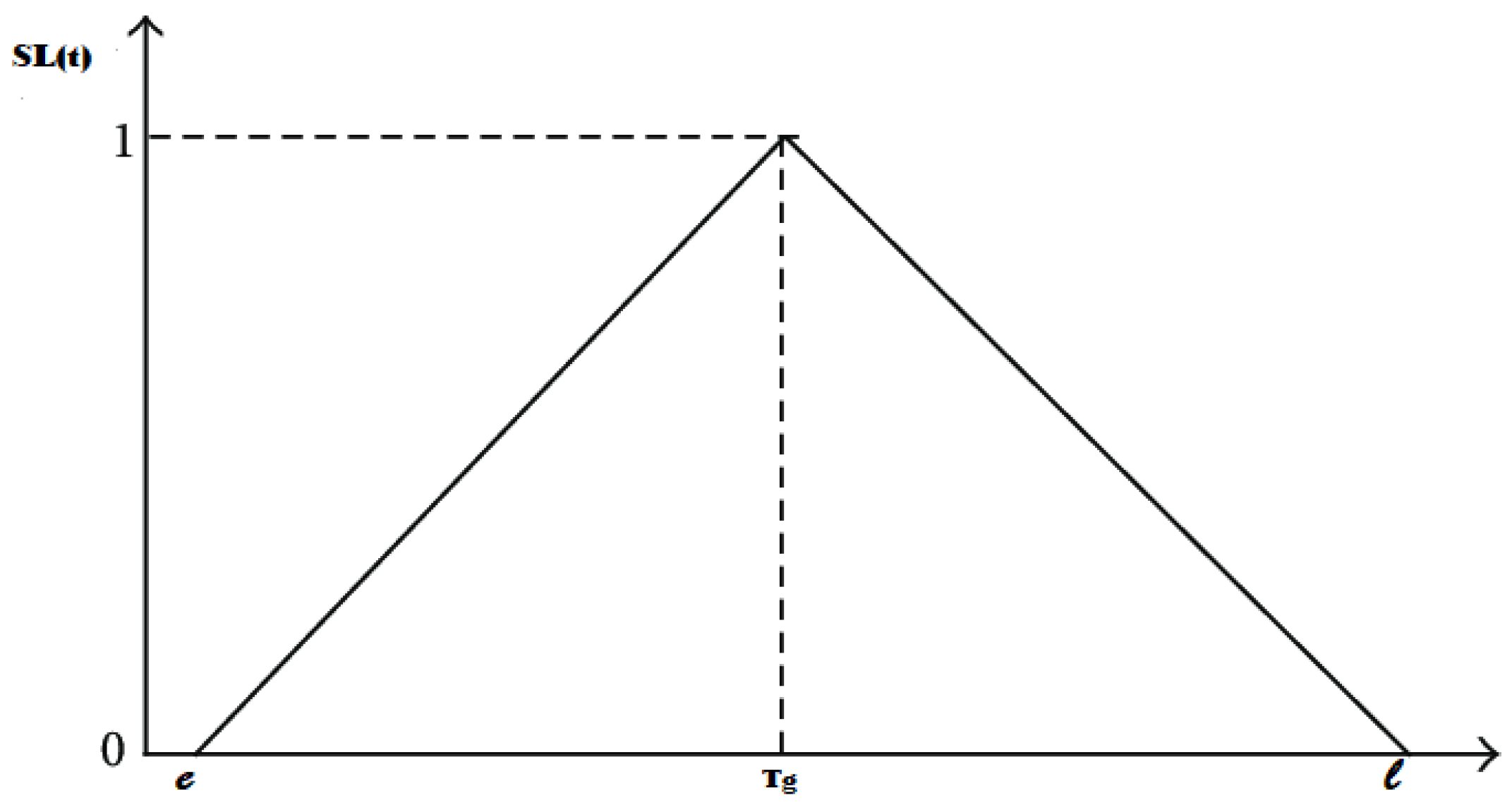
Our research was motivated by the real life distribution problem of perishable food. Indeed, customers may prefer to receive the products at a specific time in order to start preparing meals for example. In addition, restaurants tend to implement the Just In Time inventory management strategy to reduce the storage cost. Thus, instead of serving the customers within a time window, we focus on fulfilment of customer requests as much as we can at a specific target time. To assess the service level, we use the target time as an indicator by means of the following function:
Function , shown in Figure 1, represents the service level ensured for customer i if we deliver their demand at time t. is the target time, and are, respectively, the lower, and upper bounds of the time window.
The function f is non-decreasing, while g is a decreasing function that are defined as follows:
Thus, the objective is to maximize the following function:
- Objective 4: Minimize the total tardiness
In this work, we study a customer-centric version of routing problems which focus on customer satisfaction. In this variant, we consider serving the customers according to priority level. Such a problem arises when customers have different levels of attention. The motivation behind including priority indexes to our problem is that a customer may have a set of locations to be serviced, and preferences to serve each node. Priorities of customers can be defined by the decision-maker. We assume that we have a pre-defined priorities. To consider priority indexes, we define a precedence matrix P, where indicate that the customer i should be supplied before the customer j, and if customer i might be supplied after customer j.
The aim is to reduce overall tardiness as much as possible. The latter arises when a lower-priority customer is served before a higher-priority customer; these customers are either on the same route, or served by two different vehicles. In other words, the arrival time of a vehicle at a customer with lower priority () is less than the arrival time of a vehicle at a customer with higher priority (), with . The arising tardiness in this case can be denoted , and can be expressed as the difference between arrival times (when , with ) as follows:
Therefore the tardiness of the system can be computed using the following formula:
3.2. Mathematical Model
Giving the parameters, decision variables, and the objectives described above, the problem can be formulated as a Mixed integer Program (MIP) as follows:
subject to:
The objectives (17)–(20) correspond, respectively, to, minimize the total cost, maximize the average freshness, maximize the service level, and minimize the total tardiness. Constraint (21) avoids going from a point to itself. Constraint (22) avoids going from the depot to node , which represents the depot. Constraint (23) states only one vehicle visits each customer exactly once. Constraint (24) and (25) indicate the flow balance of input and output in each node. They state that for every truck and for every served client i there is at most one client j such that the truck traverses the arc . The vehicle depart from the depot 0, and return to the depot node according to the Constraint (26) and (27). Constraint (28) guarantees the respect of vehicle loading capacity. Constraint (29) establishes the relationship between the service starting times at a customer and its successor. Constraint (30) is the time window constraint. The maximum number of routes is controlled by Constraint (31) to guarantee that the number of trucks departing from the depot do not exceed the available fleet of trucks .
4. The Solving Strategy
The problem under study is a many-objectives optimization problem. As the objectives are conflicting, finding a single optimal solution is not possible. Instead, there is a set of optimal solutions.Therefore, the decision maker has to settle on the importance of each objective at some stage, in order to come up with a single solution.
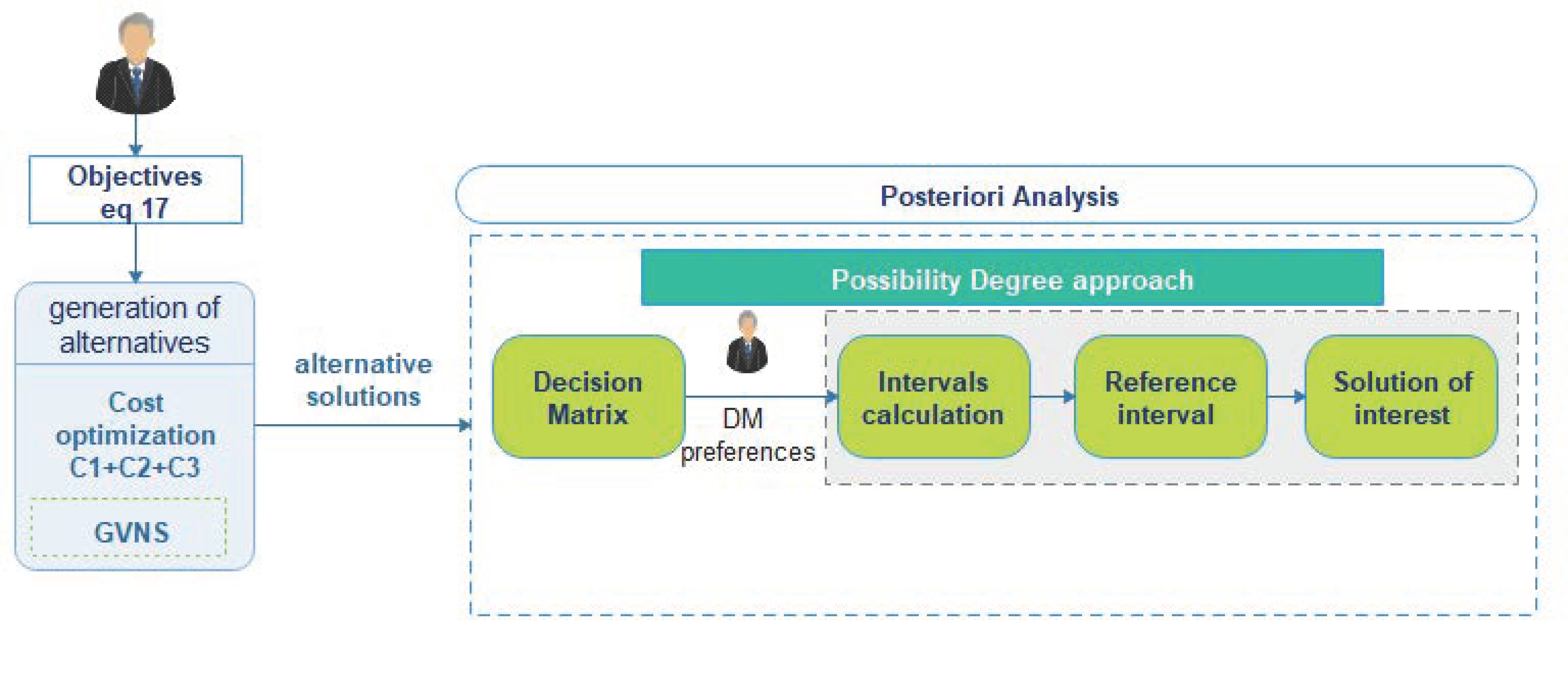
The idea of this paper is to articulate the preferences after the optimization process as an a posteriori approach. To the best of our knowledge, there is no effective tool that can deal with the problem on its original form, considering simultaneously all the objectives. Therefore, we propose to follow the steps described in the workflow diagram of Figure 2. We start by solving a sub-problem using General Variable Neighbourhood Search (GVNS) by considering a single objective (17). Afterwards, we exploit the fact that meta-heuristics can generate a set of alternative solutions. These alternatives are good with respect to the modelled objective, and expected to perform relatively well with respect to unconsidered objectives (the average freshness, the service level, and the tardiness).
The alternative solutions provided by the GVNS will be then ranked using the possibility degree approach proposed in [30], allowing the DM to choose the best solution with respect to their preferences for each criteria. The proposed ranking approach consists of assigning an interval to each solution, where the intervals correspond to the potential scores depending on the DM preferences. The solutions are then ranked through comparing their corresponding intervals using the possibility degree. The steps of the possibility degree approach are described in Appendix B. For further details, you can refer to [30].
5. General Variable Neighborhood Search Heuristic
Inspired by the successful application of variable neighbourhood search (VNS) heuristics in solving vehicle routing problem, we propose a General Variable Neighbourhood Search (GVNS) to solve the problem in hand. In this section, we begin describing the VNS and the basic details of the proposed GVNS (additional details can be found in Appendix A).
5.1. Variable Neighborhood Search (VNS)
VNS is a trajectory based-meta-heuristic proposed in [31] to solve combinatorial and global optimization problems. The method’s key principle is to adjust neighbourhoods in a systematic manner in order to arrive at an optimal (or near-optimal) solution. The VNS heuristic is made-up of three major phases: neighbour generation, local search, and jump.
Let , be the neighbourhood structures, and let denote the set of solutions in the k-th order neighbourhood of a solution x. The first step known as the shaking or diversification phase, consists of applying a neighbour of the current solution is applied. Afterwards, by applying a local search to , a solution is obtained. Finally, the current solution jumps from x to in case the latter improved the former. Otherwise, the neighbourhood’s order is incremented, and all the steps are repeated unless a stopping criteria is met.
In the field of vehicle routing problems, VNS and its variants have been widely used and recognized as efficient for solving such hard optimization problems. As examples, we can mention a VNS for a multi-depots VRP with time windows [32], a guided VNS for a large scale VRP [33], a RVNS to solve the VRPTW [34], and a VNS for periodical VRP [35].
5.2. GVNS Implementation Details
In GVNS, Variable Neighbourhood Descent (VND) is used for local search. When designing a GVNS, one should take the following design decisions: the number of neighbourhood structures, the order in which they will be explored, how the initial feasible solution is generated, the acceptance criterion and the stopping conditions. These elements define the configuration of the GVNS.
The main steps of GVNS are shown in Algorithm 1. GVNS starts by an initialization phase (line 1) in which a feasible solution is generated. The best solution is set as the first feasible solution (line 2). After selecting the neighbourhood structures for the shaking stage , and for local search (line 3), the stopping condition is then chosen (line 4). The stopping condition corresponds to a number of iterations M that will be set in the computational experience. The loop corresponding to lines 4–25 is repeated M times. The shaking process (line 8), the local search (line 9), and the move decision (line 19) are repeated until . In the shaking phase a solution is generated randomly at the neighbourhood of . Then the local search is performed to find a better solution from using the neighbourhood structures.
| Algorithm 1: GVNS |
 |
Remaining details are available in Appendix A.
6. GVNS Performance Evaluation
This section reports the computational experiments done to evaluate the efficiency of the proposed GVNS. The results are compared against those provided by an exact method (CPLEX) on a subproblem of the original model.
6.1. Data Description
To assess the performance of the proposed GVNS algorithm we conduct computational experiments on a subset of the well-known Solomon instances (https://www.sintef.no/projectweb/top/vrptw/solomon-benchmark/ (accessed on 20 August 2021)). These instances, originally developed for the classical vehicle routing problem with time window are modified to fit our problem. They are, in total, 56 instances that are classified into six categories. In our case, we test on the following categories: R1, RC1, and C1. In R1 customers locations are generated randomly; in C1 instances have clustered distributions of customers, while in RC1 instances have semi-clustered with a mix of clustered and randomly distributed customers. We conduct experiments on the following selected instances: R101, C104, and RC107. We denote the instances as in the following example: R101-20 is the instance of class ‘R1’ with 20 customers.
The parameters of the algorithm are set to the following values: . The stopping criteria M which correspond to the number of iterations, is fixed to 10. The experiments were carried out on an Intel Core i7 processor with 1.99 GHz speed and 8 GB RAM.
6.2. Computational Experiments
Using a a sub-model of the MIP problem presented before, we run a set of experiments to test the GVNS efficiency.
The submodel is:
Subject to:
The GVNS algorithm was coded in Python and the mathematical model was coded in the OPL modelling language, and solved with the CPLEX optimization solver. For CPLEX, we set the run time limit to 900 (s).
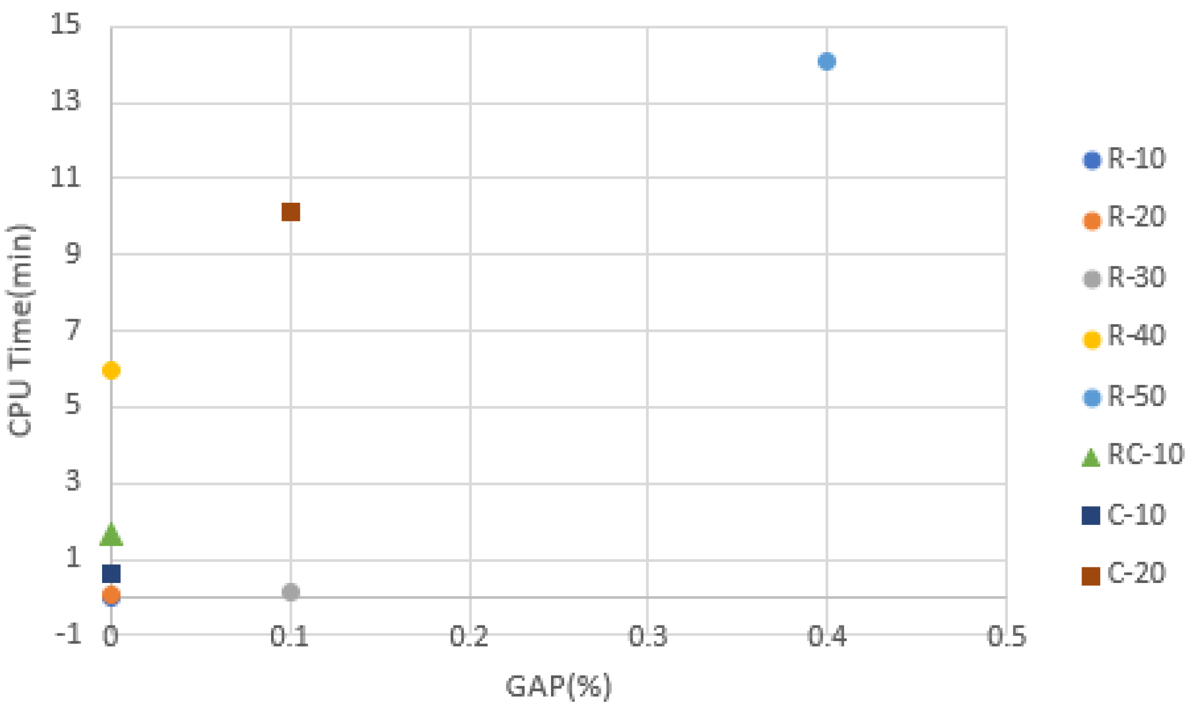
Table 3 provides the best results obtained by GVNS (out of 10 runs), the CPLEX solutions, and also the percentage gaps between both solutions. The GAP is calculated as follows:
The results indicates that our algorithm achieved the same objective value as CPLEX in 4 instances (R101-10, R101-20, R101-40, RC107-10). Furthermore, CPLEX failed to solve 22 instances within the time limit. The CPU time consumed by GVNS is less than the time spent by CPLEX. This can be clearly identified in Figure 3.
7. Application Example
Once verified the efficiency of the GVNS, we provide here a complete example of the proposed solving approach, shown in Figure 2. This section reports the test instance used, the computational experiments performed, and the results obtained.
7.1. Data and Parameter Setting
The proposed approach is applied to identify the solutions of interest for a set of 100 customers. For the data, we conduct experiments on the the category RC101 of Solomon’s instance presented in Section 6.1, that we adapted to our problem. For setting the customer’s target time, we assume that it’s the midpoint of the corresponding time window. The refrigerated vehicles used to deliver products have a fixed cost of EUR 25, and the fuel consumption is estimated to be 3 EUR/km. For the GVNS parameters, we use the same as in previous experiment Section 6.1. The other parameters are given in Table 4.
7.2. Generation of Alternative Solutions
We ran our GVNS metaheuristic 9 times to obtain the alternative solutions reported in Table 5. The algorithm provides only the total cost for each solution. Afterwards, we compute the average freshness, the service level, and the tardiness corresponding to each alternative solution. We can observe that the total cost varies between 17,966.3 and 18,323.9, the average freshness between 58.64 and 62.17, the service level from 25.71 to 30.17, and the total tardiness varies from 1,328,918 and 1,716,339.
Table 5 can be understood as a decision matrix, where solutions (1–9) are the alternatives among which the DM have to choose, and the total cost, average freshness, service level, and tardiness are the criteria for which the performance of alternatives is measured.
7.3. Decision Maker Preferences and Ranking of Solutions
At this point, the preferences of the decision maker should be considered to rank the alternatives. These will be done using scores intervals and the possibility degree approach described in Appendix B.
The preferences are established through a linear ordering of the criteria and every order corresponds to a DM profile. We define the following three profiles:
- Economic-centric (E-c): Cost Average freshness Service level Tardiness.
- Product-centric (P-c): Average freshness Cost Service level Tardiness.
- Customer Satisfaction-centric (C-c): Service level Cost Average freshness Tardiness.
where the symbol should be read as “at least as preferred to”.
The rankings of solutions under the three profiles are shown in Table 6.
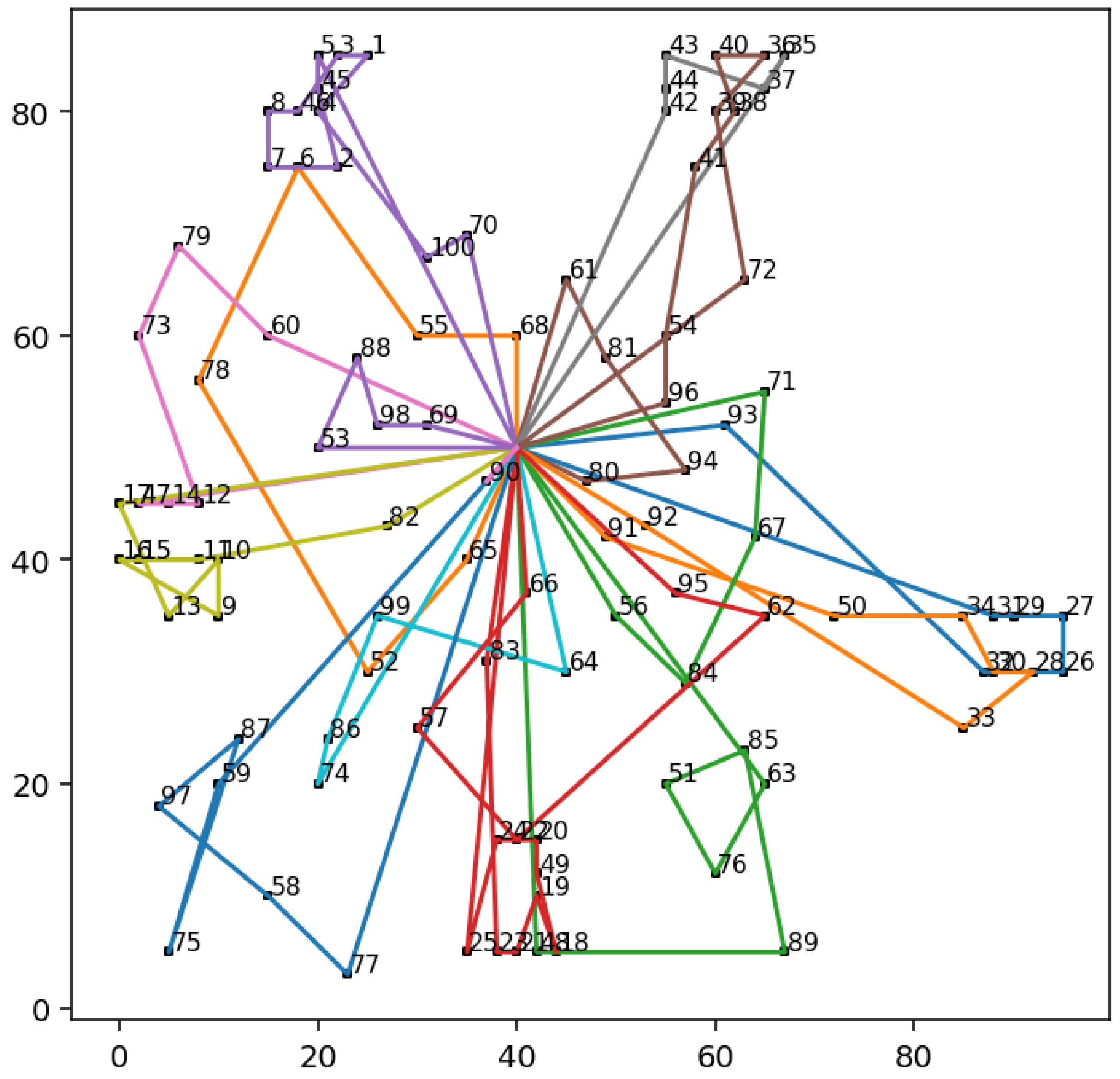
The results show that every profile lead to a different rank of the solutions. Analysing the highly ranked alternative over different scenarios, we can note that the solution presented in Figure 4 retain the first position among all scenarios. For the second-ranked alternatives, retain the position for both economic and customer-centric scenarios. However, there is a rank reversal for the profile P-c, where the alternative moves to the second position. We can also notice that and interchange their positions in profiles P-c and C-c.
By analysing the top-ranked solution represented in Figure 4, we found that 13 vehicles are used to deliver the products under customer requirements. Furthermore, we observe many arcs crossing in the tours. Indeed, in the literature, many solving strategies for VRP are based on crossing avoidance hypothesis, which is stated in [36,37]. However, crossing arcs appeared in our solutions due to customers requirement ( time windows, priority indexes).
8. Conclusions and Perspectives
In this paper, we propose a many objective customer-centric Perishable Food Distribution Problem and a strategy to solve it. The model distinguishes four objectives: minimize the overall cost, maximize the average freshness of products, maximize the service level by fulfilling the customer demand within the time range required, and in the target time if possible. We also minimize the tardiness of the system resulted from the non-respect of customer’s priority.
To solve the problem, we propose a strategy that starts by solving a sub-problem considering only the cost minimization objective, using a General Variable Neighbourhood Search algorithm (GVNS). The performance of GVNS in the sub-problem is compared against an exact method (CPLEX) allowing us to conclude that the method is efficient.
Moreover, the algorithm generates a set of diverse solutions that are then evaluated to integrate the other criteria (average freshness, service level, tardiness). To come up with a single solution of interest for the decision maker among those generated by the GVNS, we used score intervals and a possibility degree approach allowing the DM to rank the set of alternatives solutions based on his/her preferences. The combination of GVNS and the possibility degree approach is tested on a full example that allows to assess the impact of criteria preferences on the solutions ranking.
Future work will be devoted to further explore the use of GVNS like methods as candidate solutions generators and to study how to address environmental features in the model like congestion of the routes and/or reducing CO2 emissions.
Author Contributions
Conceptualization and Methodology, D.A.P., H.E.R. and M.O.; software, H.E.R.; investigation, D.A.P., H.E.R., M.O. and A.E.H.A.; writing—review and editing, D.A.P., H.E.R. and M.O. All authors have read and agreed to the published version of the manuscript.
Funding
The CNRST has awarded H. El Raoui an excellence scholarship. D. Pelta acknowledges support from projects TIN2017-86647-P (Spanish Ministry of Economy, Industry, and Competitiveness. Including FEDER funds) and PID2020-112754GB-I00 (Spanish Ministry of Science and Innovation).
Conflicts of Interest
The authors declare no conflict of interest.
Appendix A. The General Variable Neighborhood Search GVNS
In this appendix we describe both the initial solution generation and the neighbourhood structures implemented in GVNS.
Appendix A.1. Initial Solution Generation
Solution construction refers to the creation of a set of routes for the vehicles by selecting nodes (customers), and inserting them in routes already created or in a new route. The two famous types of solution construction used for VRP are the sequential construction and the parallel construction. The first feasible solution is found by the insertion heuristic called .
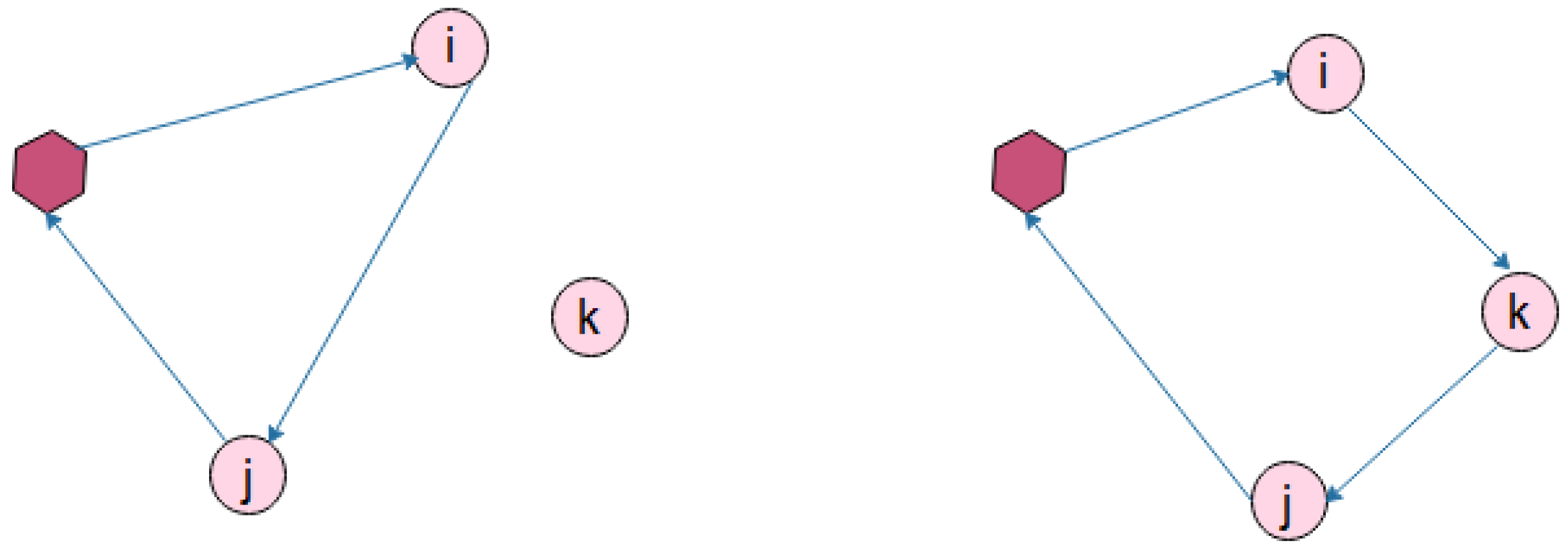
Insertion heuristic belongs to the sequential construction heuristics described by Solomon in [38]. It’s based on expanding the current initialized route by inserting unrouted customers. The main idea is described in Figure A1, where a customer k is inserted between i and j.
Figure A1.
Insertion heuristic.

The insertion heuristic initialize the route with a ‘seed’ customer, which is either the farthest from the depot or the one with the lowest allowed starting service time. In our approach, we initialize the route with the farthest customer. Afterwards, two criteria and are used to insert at each iteration an unrouted customer u into the current route, between a pair of adjacent customers i and j. Let be the current route where . For each unrouted customer u, we compute its best feasible insertion position in the route as follows:
In the literature the criterion is calculated based on the extra travel time, and the extra euclidean distance resulted after the insertion of customer u.
where
, and are, respectively, the distances between customers iu, uj, and ij. denotes the new starting service time at customer j, and is the starting service time at j before inserting u. The distance savings are regulated by the Parameter . Following that, the best node to insert in the route is chosen based on the second criteria as the one for which
u is unrouted and the route is feasible.
Unless all unrouted customers are inserted, the algorithm initiates a new route when no more feasible insertions are found.
The criterion is computed as follows:
where is a parameter used to specify how much the best insertion position for an unrouted customer is affected by the distance from the depot . On the other hand defines how much the best place depends on the extra distance and the time needed to visit the customer by the current vehicle.
Appendix A.2. The Neighbourhood Structures
The choice of neighbourhood structures and the order in which we explore them is of crucial importance. Indeed, local search methods sequentially accept solutions that improve the objective function value. Thus, the solution quality depends heavily on initial solutions and the neighbourhood structure NS. The NS can be based on several moves (operators). The following terms are employed: inter-route, and intra-route.
Intra-route operator make moves within one route in order to reduce the travel cost, while inter-route operator make moves between two separate routes.
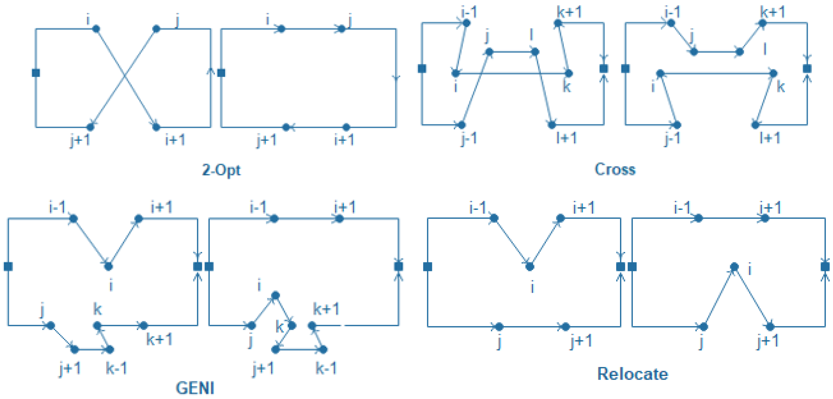
We used in our approaches four neighbourhood structures corresponding to moves presented in Figure A2, in the following order: GENI, CROSS, 2-OPT, RELOCATE. This order is based on cardinality, which implies moving from relatively poor to richer neighbourhood structures [39].
Figure A2.
Description of the basic move operators.

We note that generally in the literature, the neighbourhood structures NS used in the shaking phase are different from the NS in the local search. However, we choose to use the same neighbourhood structures in both phases.
- Relocate: In this operator the customer visit is moved from a route to another.
- GENI: Is a variant of the relocate operator which consists of placing a customer two customer nodes on the closest destination path, even though they are not consecutive.
- CROSS: The key concept behind cross exchange is to remove two edges and from the first route, and remove and from the second route. Then, by adding the edges ,, , and the segments and are swapped.
- 2-OPT: Replace two of the tour’s edges with two additional edges, and iterates until no further change is necessary.
Appendix B. A Possibility Degree Based Approach to Rank Solutions
This appendix summarizes the main aspects of the approach proposed in [30], which departs from a decision matrix like
| c1 | c2 | … | cn | |
| A1 | x11 | x12 | … | x1n |
| A2 | x21 | x22 | … | x2n |
| Am | xm1 | xm2 | … | xmn |
One way to sort the alternatives is to first combine their performance values using an aggregation function in order to have a score, and second to sort them using such scores.
A basic aggregation function is the weighted aggregation, where in simple terms, the decision maker provides a set of weights and then the score of an alternative is calculated as with . If criteria is more relevant than for the decision maker, then .
Let us suppose we have just three criteria and the given preference order is . Then we need to define with . As the reader may notice, there are infinite values for that verifies both conditions and every possible set of values will give a different score for the alternative.
So instead of assigning a single score value, the proposed approach calculates an interval of the potential scores that an alternative can attain.
The main steps are detailed below.
Appendix B.1. Decision Matrix Normalization
Before applying an aggregation function, the decision matrix needs to be normalized so it becomes dimensionless and all of its elements are comparable. While there are different normalization techniques, the following method is adopted here: For benefit criteria:
For cost criteria:
Appendix B.2. Intervals Calculations
Let us assume that the DM express his/her preferences using an ordinal relation among criteria denoted as . The symbol is to be read as “at least as preferred to”. This implies that the weights are ordered as .
All the potential scores that an alternative can attain are included in the interval denoted as with are, respectively, the minimum, and the maximum scores obtained through solving two simple linear programming problems
s.t. for both problems
Appendix B.3. Reference Interval and Interval’s Comparison
At this point, every alternative has an associated interval .
Next a reference alternative and its corresponding interval are identified. Such alternative is the one with the greatest lower bound , thus there is no solution that always scores better than .
Then, every alternative is compared against using a possibility function that calculates the possibility degree of an alternative being better than another using their corresponding intervals.
Let be two non-negative interval numbers with The possibility degree of X being greater than Y namely proposed in [40] is defined as follows:
- 1.
- if
- 2.
- if
Appendix B.4. Ranking of Alternatives
Now, for every alternative the value is calculated. Then, the alternatives are sorted based on such possibility degree values.
References
- Yakavenka, V.; Mallidis, I.; Vlachos, D.; Iakovou, E.; Eleni, Z. Development of a multi-objective model for the design of sustainable supply chains: The case of perishable food products. Ann. Oper. Res. 2020, 294, 593–621. [Google Scholar] [CrossRef]
- Tuljak Suban, D.; Suban, V. Influence of transportation mode to the deterioration rate: Case study of food transport by ship. Int. J. Biol. Biomol. Agric. Biotechnol. Eng. 2015, 9, 37–42. [Google Scholar]
- Boge, F. Food Waste & Food Imperfection. 2019. Available online: http://tesi.luiss.it/24940/ (accessed on 20 August 2021).
- Utama, D.M.; Dewi, S.K.; Wahid, A.; Santoso, I. The vehicle routing problem for perishable goods: A systematic review. Cogent Eng. 2020, 7, 1816148. [Google Scholar] [CrossRef]
- Raseman, W.J.; Jacobson, J.; Kasprzyk, J.R. Parasol: An open source, interactive parallel coordinates library for multi-objective decision making. Environ. Model. Softw. 2019, 116, 153–163. [Google Scholar] [CrossRef]
- Mullaseril, P.A.; Dror, M.; Leung, J. Split-delivery routeing heuristics in livestock feed distribution. J. Oper. Res. Soc. 1997, 48, 107–116. [Google Scholar] [CrossRef]
- Tarantilis, C.; Kiranoudis, C. A meta-heuristic algorithm for the efficient distribution of perishable foods. J. Food Eng. 2001, 50, 1–9. [Google Scholar] [CrossRef]
- Tarantilis, C.; Kiranoudis, C. Distribution of fresh meat. J. Food Eng. 2002, 51, 85–91. [Google Scholar] [CrossRef]
- Faulin, J. Applying MIXALG procedure in a routing problem to optimize food product delivery. Omega 2003, 31, 387–395. [Google Scholar] [CrossRef]
- Prindezis, N.; Kiranoudis, C.; Marinos-Kouris, D. A business-to-business fleet management service provider for central food market enterprises. J. Food Eng. 2003, 60, 203–210. [Google Scholar] [CrossRef]
- Campbell, A.M.; Savelsbergh, M.W. Decision support for consumer direct grocery initiatives. Transp. Sci. 2005, 39, 313–327. [Google Scholar] [CrossRef] [Green Version]
- Ambrosino, D.; Sciomachen, A. A food distribution network problem: A case study. IMA J. Manag. Math. 2007, 18, 33–53. [Google Scholar] [CrossRef]
- Hsu, C.I.; Hung, S.F.; Li, H.C. Vehicle routing problem with time-windows for perishable food delivery. J. Food Eng. 2007, 80, 465–475. [Google Scholar] [CrossRef]
- Osvald, A.; Stirn, L.Z. A vehicle routing algorithm for the distribution of fresh vegetables and similar perishable food. J. Food Eng. 2008, 85, 285–295. [Google Scholar] [CrossRef]
- Doerner, K.F.; Gronalt, M.; Hartl, R.F.; Kiechle, G.; Reimann, M. Exact and heuristic algorithms for the vehicle routing problem with multiple interdependent time windows. Comput. Oper. Res. 2008, 35, 3034–3048. [Google Scholar] [CrossRef]
- Chen, H.K.; Hsueh, C.F.; Chang, M.S. Production scheduling and vehicle routing with time windows for perishable food products. Comput. Oper. Res. 2009, 36, 2311–2319. [Google Scholar] [CrossRef]
- Hasani, A.; Zegordi, S.H.; Nikbakhsh, E. Robust closed-loop supply chain network design for perishable goods in agile manufacturing under uncertainty. Int. J. Prod. Res. 2012, 50, 4649–4669. [Google Scholar] [CrossRef]
- El Raoui, H.; Oudani, M.; Alaoui, A.E.H. ABM-GIS simulation for urban freight distribution of perishable food. In Proceedings of the International Workshop on Transportation and Supply Chain Engineering (IWTSCE 18), Rabat, Morocco, 8–9 May 2018. [Google Scholar]
- El Raoui, H.; Oudani, M.; Pelta, D.; Alaoui, A.E.H.; El Aroudi, A. Vehicle routing problem on a road-network with fuzzy time windows for perishable food. In Proceedings of the IEEE International Smart Cities Conference (ISC2), Casablanca, Morocco, 14–17 October 2019; IEEE: New York, NY, USA, 2019; pp. 492–497. [Google Scholar]
- El Raoui, H.; Oudani, M.; Alaoui, A.E.H. Perishable food distribution in urban area based on real-road network graph. In Proceedings of the 5th International Conference on Logistics Operations Management (GOL), Rabat, Morocco, 28–30 October 2020; IEEE: New York, NY, USA, 2020; pp. 1–6. [Google Scholar]
- Gong, W.; Fu, Z. ABC-ACO for perishable food vehicle routing problem with time windows. In Proceedings of the 2010 International Conference on Computational and Information Sciences, Chengdu, China, 17–19 December 2010; IEEE: New York, NY, USA, 2010; pp. 1261–1264. [Google Scholar]
- Amorim, P.; Almada-Lobo, B. The impact of food perishability issues in the vehicle routing problem. Comput. Ind. Eng. 2014, 67, 223–233. [Google Scholar] [CrossRef]
- Govindan, K.; Jafarian, A.; Khodaverdi, R.; Devika, K. Two-echelon multiple-vehicle location–routing problem with time windows for optimization of sustainable supply chain network of perishable food. Int. J. Prod. Econ. 2014, 152, 9–28. [Google Scholar] [CrossRef]
- Khalili-Damghani, K.; Abtahi, A.R.; Ghasemi, A. A new bi-objective location-routing problem for distribution of perishable products: Evolutionary computation approach. J. Math. Model. Algorithms Oper. 2015, 14, 287–312. [Google Scholar] [CrossRef]
- Kuo, R.; Nugroho, D.Y. A fuzzy multi-objective vehicle routing problem for perishable products using gradient evolution algorithm. In Proceedings of the 2017 4th international conference on industrial engineering and applications (ICIEA), Nagoya, Japan, 21–23 April 2017; IEEE: New York, NY, USA, 2017; pp. 219–223. [Google Scholar]
- Sahraeian, R.; Esmaeili, M. A multi-objective two-echelon capacitated vehicle routing problem for perishable products. J. Ind. Syst. Eng. 2018, 11, 62–84. [Google Scholar]
- Zulvia, F.E.; Kuo, R.; Nugroho, D.Y. A many-objective gradient evolution algorithm for solving a green vehicle routing problem with time windows and time dependency for perishable products. J. Clean. Prod. 2020, 242, 118428. [Google Scholar] [CrossRef]
- Wang, S.; Tao, F.; Shi, Y.; Wen, H. Optimization of vehicle routing problem with time windows for cold chain logistics based on carbon tax. Sustainability 2017, 9, 694. [Google Scholar] [CrossRef] [Green Version]
- Wang, X.; Wang, M.; Ruan, J.; Li, Y. Multi-objective optimization for delivering perishable products with mixed time windows. Adv. Prod. Eng. Manag. 2018, 13, 321–332. [Google Scholar] [CrossRef] [Green Version]
- Torres, M.; Pelta, D.A.; Lamata, M.T.; Yager, R.R. An approach to identify solutions of interest from multi and many-objective optimization problems. Neural Comput. Appl. 2021, 33, 2471–2481. [Google Scholar] [CrossRef]
- Mladenović, N.; Hansen, P. Variable neighborhood search. Comput. Oper. Res. 1997, 24, 1097–1100. [Google Scholar] [CrossRef]
- Polacek, M.; Hartl, R.F.; Doerner, K.; Reimann, M. A variable neighborhood search for the multi depot vehicle routing problem with time windows. J. Heuristics 2004, 10, 613–627. [Google Scholar] [CrossRef] [Green Version]
- Kytöjoki, J.; Nuortio, T.; Bräysy, O.; Gendreau, M. An efficient variable neighborhood search heuristic for very large scale vehicle routing problems. Comput. Oper. Res. 2007, 34, 2743–2757. [Google Scholar] [CrossRef]
- Goel, A.; Gruhn, V. A general vehicle routing problem. Eur. J. Oper. Res. 2008, 191, 650–660. [Google Scholar] [CrossRef] [Green Version]
- Hemmelmayr, V.C.; Doerner, K.F.; Hartl, R.F. A variable neighborhood search heuristic for periodic routing problems. Eur. J. Oper. Res. 2009, 195, 791–802. [Google Scholar] [CrossRef] [Green Version]
- Fontaine, P.; Taube, F.; Minner, S. Human solution strategies for the vehicle routing problem: Experimental findings and a choice-based theory. Comput. Oper. Res. 2020, 120, 104962. [Google Scholar] [CrossRef]
- Van Rooij, I.; Stege, U.; Schactman, A. Convex hull and tour crossings in the Euclidean traveling salesperson problem: Implications for human performance studies. Mem. Cogn. 2003, 31, 215–220. [Google Scholar] [CrossRef] [PubMed] [Green Version]
- Solomon, M.M. Algorithms for the vehicle routing and scheduling problems with time window constraints. Oper. Res. 1987, 35, 254–265. [Google Scholar] [CrossRef] [Green Version]
- Bräysy, O.; Gendreau, M. Vehicle routing problem with time windows, Part I: Route construction and local search algorithms. Transp. Sci. 2005, 39, 104–118. [Google Scholar] [CrossRef] [Green Version]
- Liu, F.; Pan, L.H.; Liu, Z.L.; Peng, Y.N. On possibility-degree formulae for ranking interval numbers. Soft Comput. 2018, 22, 2557–2565. [Google Scholar] [CrossRef]
Figure 1.
The service level function.

Figure 2.
Graphical depiction of the solving strategy.

Figure 3.
The GAP and CPU time difference between GVNS and CPLEX for every exactly solved instance.

Figure 4.
The Top-Ranked solution represented on graph.


Table 1.
A review of the papers solving perishable food distribution problem.
| References | Sustainability Aspect | Sustainability Measure | Objective Functions | Methods | ||
|---|---|---|---|---|---|---|
| Economic | Environmental | Social | ||||
| [6] | * | * | Distribution cost Time window respect | Min. total cost | Heuristics | |
| [7] | * | Distribution cost | Min. travel cost | Heuristics | ||
| [8] | * | Distribution cost | Min. travel cost | Heuristics | ||
| [9] | * | Distribution cost | Min. total distance | Heuristics+ Exact | ||
| [10] | * | Distribution cost | Min. total cost | Metaheuristics | ||
| [11] | * | Profitability | Max. profit | Heuristics | ||
| [12] | * | Distribution cost | Min. total cost | Heuristics | ||
| [13] | * | * | Distribution cost Time window respect | Min. total cost | Heuristic | |
| [14] | * | * | Distribution cost Products quality | Min. total cost | Heuristics | |
| [15] | * | * | Cost efficiency Time window respect | Min. total distance | Exact+ Heuristics | |
| [16] | * | * | Cost efficiency Products quality Time window respect | Max. profit | Exact+ Heuristics | |
| [17] | * | * | Cost efficiency Products quality | Max. profit | Exact | |
| [18] | * | * | * | Cost efficiency Time window respect Carbon emission | Min. total travel time | Simulation |
| [19] | * | * | Distribution cost Time window respect | Min. total cost | Exact | |
| [20] | * | * | Distribution cost Time window respect | Min. total cost | Exact | |
| [21] | * | * | Distribution cost Products quality | Min. total cost | Heuristic | |
| [22] | * | * | Cost efficiency Products freshness Time window respect | Min. total cost Max. freshness | Mulit-objective evolutionary algorithm | |
| [23] | * | * | * | Cost efficiency Products quality Time window respect Environmental impact | Min. total cost Min. carbon emissions | Metaheuristics+ Pareto optimality |
| [24] | * | Distribution cost | Min. total cost | Evolutionary computation | ||
| [25] | * | * | Distribution cost Time window respect | Min. total cost Min. variance of vehicles | Multi-objective Gradient Evolutionary algorithm | |
| [26] | * | * | * | Cost efficiency Service level Environmental impact | Min. total cost Min. waiting time Min. carbon emissions | NSGA-II |
| [27] | * | * | * | Distribution cost Products freshness Time window respect Environmental impact | Min. operational cost Min. deterioration cost Min. carbon emission Max. service level | Many-objective Gradient Evolutionary algorithm |
Table 2.
Sets, parameters, and decision variables for model formulation.
| Sets and Indices | |
| V | Set of nodes |
| Set of customers | |
| K | Set of vehicles |
| i,j | Indices of nodes |
| Decision Variables | |
| A 0-1 decision variable, equal to 1 in case the truck k travels from node i to j, 0 otherwise. | |
| A 0-1 decision variable, equal to 1 in case the customer i is served by the truck k, 0 otherwise. | |
| A decision variable representing the starting service time at node i using the truck k. | |
| Parameters | |
| The transportation cost from node i to j. | |
| F | Fixed cost associated to a vehicle. |
| The travel time from i to j. | |
| The distance between node i and j. | |
| The cost per unit time for the refrigeration during the transportation process. | |
| The unloading time at customer i. | |
| The unit refrigeration cost during the unloading. | |
| The necessary time to serve customer i | |
| The demand of customer i | |
| P | The price per unit product |
| The products remaining on the vehicle after serving the customer i | |
| Q | The loading capacity of trucks. |
| K | The fleet of trucks |
| The spoilage rate of products during the transportation process | |
| The spoilage rate of products during the unloading process | |
| The time window of customer i | |
| The target time of customer i | |
| The service level for customer i if we deliver their demand at time t. | |
| M | Large positive constant. |
Table 3.
Comparison between best GVNS and CPLEX solutions.
| Instance | GVNS Solution | CPLEX Solution | Gap (%) | ||
|---|---|---|---|---|---|
| Objective | Time (s) | Objective | Time (s) | ||
| R101-10 | 630.52 | 0.04 | 630.520 | 1.76 | 0 |
| R101-20 | 1224.18 | 3.59 | 1224.18 | 7.15 | 0 |
| R101-30 | 1665.78 | 3.64 | 1664.10 | 11.20 | 0.1 |
| R101-40 | 2223.10 | 6.51 | 2223.10 | 363.00 | 0 |
| R101-50 | 2600.48 | 14.36 | 2589.92 | 858.00 | 0.4 |
| R101-60 | 2969.64 | 26.44 | No Sol | ||
| R101-70 | 3543.04 | 35.74 | No Sol | ||
| R101-80 | 3794.16 | 51.77 | No Sol | ||
| R101-90 | 4159.70 | 84.99 | No Sol | ||
| R101-100 | 4398.88 | 111.70 | No Sol | ||
| RC107-10 | 436.32 | 0.06 | 436.32 | 1.74 | 0 |
| RC107-20 | 771.70 | 1.45 | No Sol | ||
| RC107-30 | 1147.52 | 4.09 | No Sol | ||
| RC107-40 | 1469.18 | 8.21 | No Sol | ||
| RC107-50 | 1860.02 | 20.33 | No Sol | ||
| RC107-60 | 2434.92 | 45.78 | No Sol | ||
| RC107-70 | 2657.12 | 180.10 | No Sol | ||
| RC107-80 | 3023.60 | 249.30 | No Sol | ||
| RC107-90 | 3401.92 | 358.50 | No Sol | ||
| RC107-100 | 3591.20 | 589.60 | No Sol | ||
| C104-10 | 1068.34 | 0.01 | 1068.34 | 0.65 | 0 |
| C104-20 | 2121.10 | 5.02 | 2118.96 | 15.15 | 0.1 |
| C104-30 | 3111.16 | 23.75 | No Sol | ||
| C104-40 | 4279.34 | 51.13 | No Sol | ||
| C104-50 | 5228.74 | 75.10 | No Sol | ||
| C104-60 | 6341.10 | 69.57 | No Sol | ||
| C104-70 | 7572.30 | 151.30 | No Sol | ||
| C104-80 | 8591.68 | 590.80 | No Sol | ||
| C104-90 | 9636.78 | 777.90 | No Sol | ||
| C104-100 | 10740.60 | 943.40 | No Sol | ||
Table 4.
Problem parameters setting.
| Parameter | Value |
|---|---|
| P | 20 EUR/Unit |
| 0.002 | |
| 0.003 | |
| 0.03 EUR/unit | |
| 0.04 EUR/unit | |
| 0.8 |
Table 5.
The set of alternative solutions.
| Total Cost | Average Freshness | Service Level | Tardiness | |
|---|---|---|---|---|
| 18,294.37 | 62.17 | 29.02 | 1,455,295 | |
| 18,323.90 | 58.64 | 25.71 | 1,621,316 | |
| 18,256.38 | 62.02 | 30.06 | 1,498,330 | |
| 18,120.14 | 61.03 | 28.32 | 1,716,339 | |
| 18,277.78 | 62.12 | 30.71 | 1,328,918 | |
| 18,011.75 | 61.74 | 27.91 | 1,504,620 | |
| 18,179.60 | 61.08 | 27.16 | 1,467,776 | |
| 18,013.66 | 61.76 | 27.51 | 1,480,522 | |
| 17,966.30 | 61.66 | 26.87 | 1,562,182 |
Table 6.
Ranking of solutions for every DM profile.
| Rank | 1 | 2 | 3 | 4 | 5 | 6 | 7 | 8 | 9 |
|---|---|---|---|---|---|---|---|---|---|
| E-c | |||||||||
| P-c | |||||||||
| C-c |
Publisher’s Note: MDPI stays neutral with regard to jurisdictional claims in published maps and institutional affiliations. |
© 2021 by the authors. Licensee MDPI, Basel, Switzerland. This article is an open access article distributed under the terms and conditions of the Creative Commons Attribution (CC BY) license (https://creativecommons.org/licenses/by/4.0/).
Share and Cite
MDPI and ACS Style
El Raoui, H.; Oudani, M.; Pelta, D.A.; El Hilali Alaoui, A. A Metaheuristic Based Approach for the Customer-Centric Perishable Food Distribution Problem. Electronics 2021, 10, 2018. https://doi.org/10.3390/electronics10162018
AMA Style
El Raoui H, Oudani M, Pelta DA, El Hilali Alaoui A. A Metaheuristic Based Approach for the Customer-Centric Perishable Food Distribution Problem. Electronics. 2021; 10(16):2018. https://doi.org/10.3390/electronics10162018
Chicago/Turabian StyleEl Raoui, Hanane, Mustapha Oudani, David A. Pelta, and Ahmed El Hilali Alaoui. 2021. "A Metaheuristic Based Approach for the Customer-Centric Perishable Food Distribution Problem" Electronics 10, no. 16: 2018. https://doi.org/10.3390/electronics10162018
Note that from the first issue of 2016, this journal uses article numbers instead of page numbers. See further details here.