
Recurrent Neural Network for Human Activity Recognition in Embedded Systems Using PPG and Accelerometer Data

 , , and
Abstract
:1. Introduction
- We design an RNN using PPG and triaxial accelerometer data in order to detect human activity, using a publicly available data set for its design and testing. The design and hyper-parameter optimization is performed on a computer architecture.
- After the RNN has been designed, we investigate the porting and performance of the network on an embedded device, namely the STM32 microcontroller architecture from ST, using their “STM32Cube.AI” software solution [41]. This framework allows the porting of a pre-built DNN, converting it to optimized code to be run on the constrained hardware platform.
- When porting the RNN to the embedded system, we show how the network can be simplified to better fit the microcontroller limited resources. In particular, it is demonstrated that the input data can be downsampled to a significant degree, while maintaining good accuracy and requiring fewer hardware resources in order to be implemented.
2. Related Work
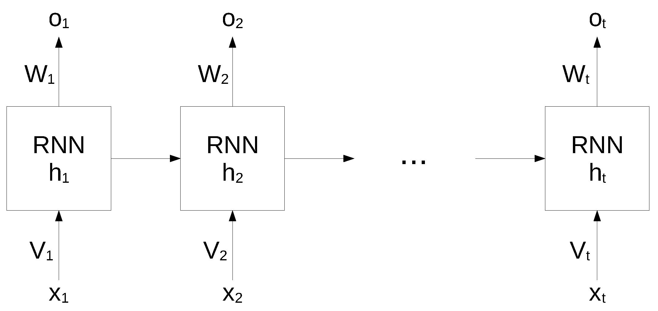
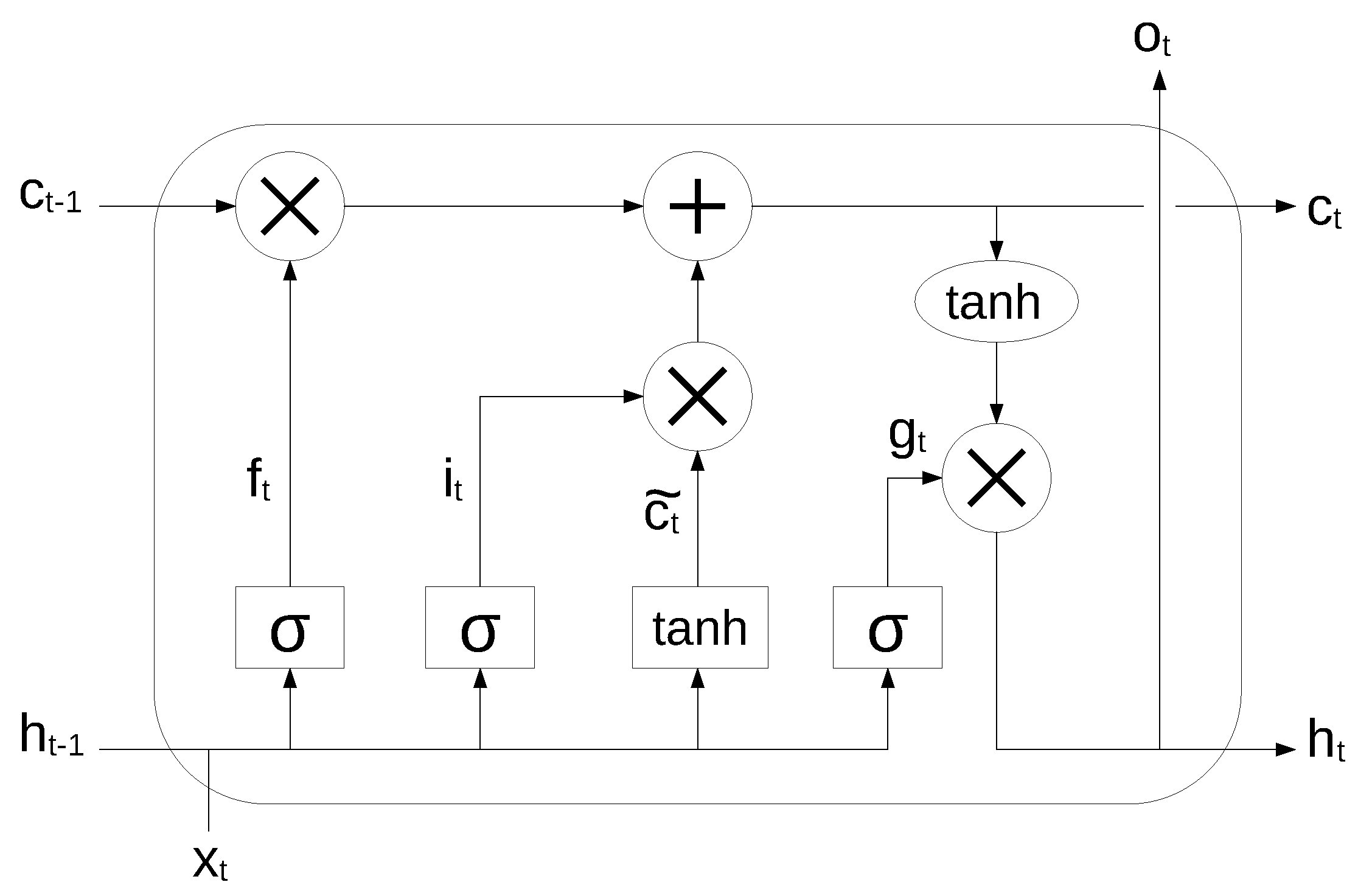
3. Brief of RNNs
4. Data Set
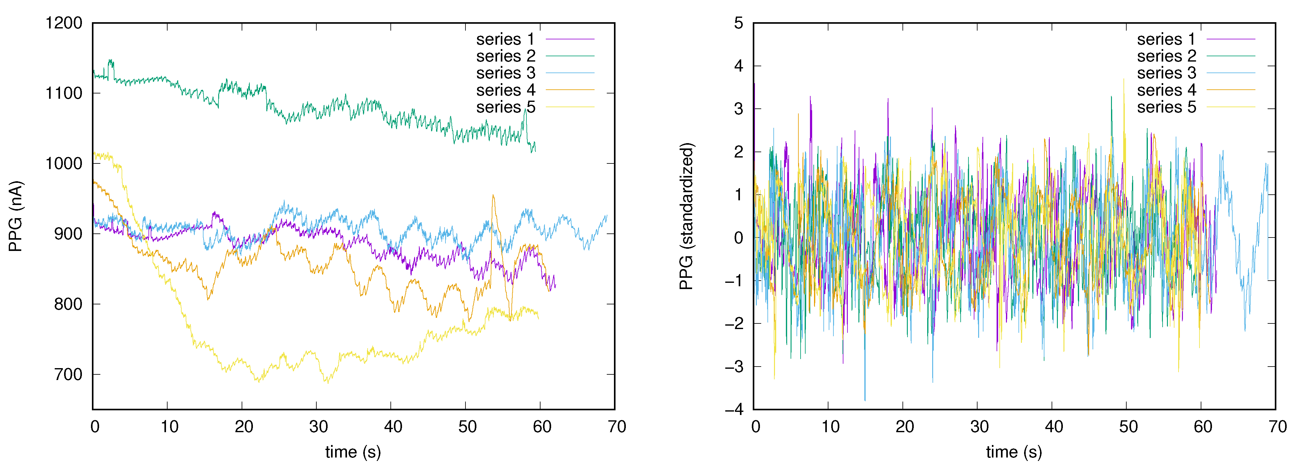
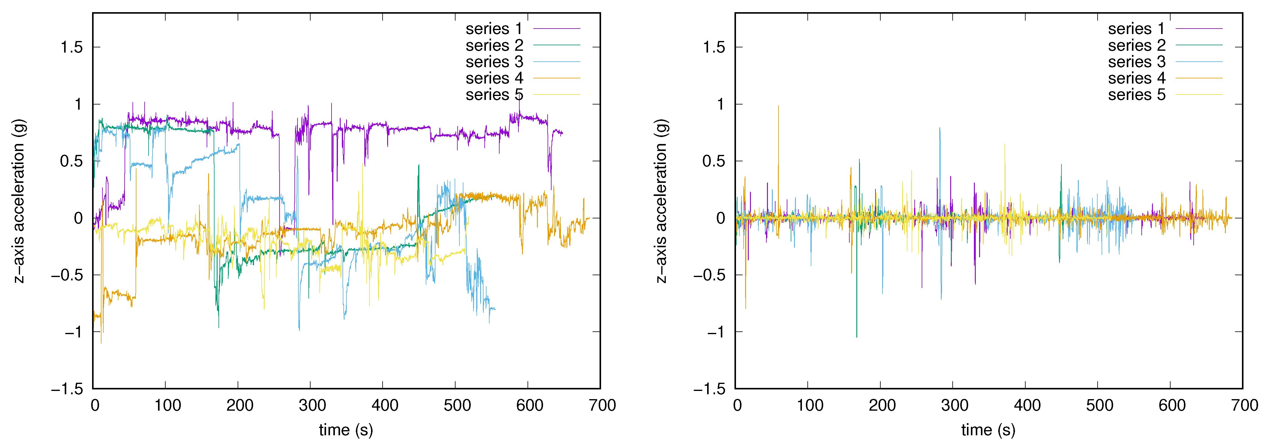
4.1. Data Pre-Processing
4.2. Data Downsampling
4.3. Data Windowing
4.4. Data Augmentation
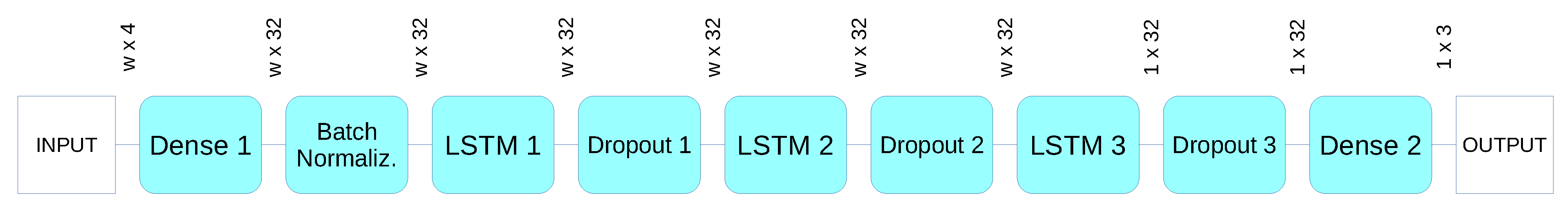
5. Rnn Architecture
5.1. Hardware and Software
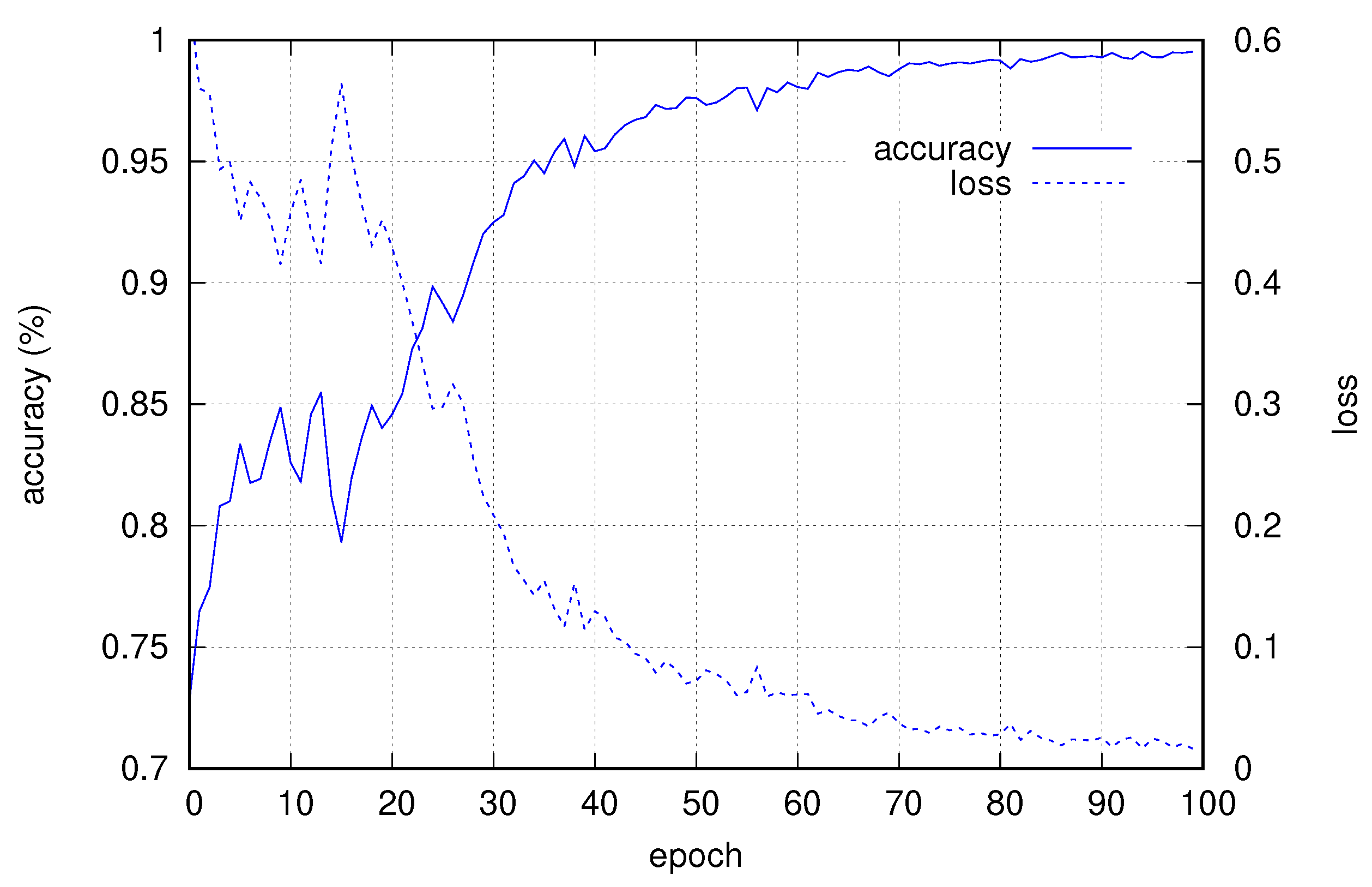
6. Experimental Results
- Windows of 1200 samples (before decimation) and 50% overlapping.
- Data augmentation applied.
- Five subjects used for training, with no further split for validation.
- Test performed on the last two subjects, not involved in training.
- A total of 100 training epochs.
7. Conclusions
Author Contributions
Funding
Data Availability Statement
Conflicts of Interest
References
- Cicirelli, F.; Fortino, G.; Giordano, A.; Guerrieri, A.; Spezzano, G.; Vinci, A. On the design of smart homes: A framework for activity recognition in home environment. J. Med. Syst. 2016, 40, 1–17. [Google Scholar] [CrossRef]
- Rashidi, P.; Cook, D.J. Keeping the resident in the loop: Adapting the smart home to the user. IEEE Trans. Syst. Man Cybern. Part A Syst. Hum. 2009, 39, 949–959. [Google Scholar] [CrossRef]
- Boukhechba, M.; Chow, P.; Fua, K.; Teachman, B.A.; Barnes, L.E. Predicting social anxiety from global positioning system traces of college students: Feasibility study. JMIR Ment. Health 2018, 5, e10101. [Google Scholar] [CrossRef]
- Boukhechba, M.; Daros, A.R.; Fua, K.; Chow, P.I.; Teachman, B.A.; Barnes, L.E. DemonicSalmon: Monitoring mental health and social interactions of college students using smartphones. Smart Health 2018, 9, 192–203. [Google Scholar] [CrossRef]
- Patel, S.; Park, H.; Bonato, P.; Chan, L.; Rodgers, M. A review of wearable sensors and systems with application in rehabilitation. J. Neuroeng. Rehabil. 2012, 9, 1–17. [Google Scholar] [CrossRef] [Green Version]
- Avci, A.; Bosch, S.; Marin-Perianu, M.; Marin-Perianu, R.; Havinga, P. Activity recognition using inertial sensing for healthcare, wellbeing and sports applications: A survey. In Proceedings of the 23th International Conference on Architecture of Computing Systems 2010, VDE, Hannover, Germany, 22–25 February 2010; pp. 1–10. [Google Scholar]
- Mazilu, S.; Blanke, U.; Hardegger, M.; Tröster, G.; Gazit, E.; Hausdorff, J.M. GaitAssist: A daily-life support and training system for parkinson’s disease patients with freezing of gait. In Proceedings of the SIGCHI conference on Human Factors in Computing Systems, Toronto, ON, Canada, 26 April–1 May 2014; pp. 2531–2540. [Google Scholar]
- Chen, L.; Wei, H.; Ferryman, J. A survey of human motion analysis using depth imagery. Pattern Recognit. Lett. 2013, 34, 1995–2006. [Google Scholar] [CrossRef]
- Taha, A.; Zayed, H.H.; Khalifa, M.; El-Horbaty, E.S.M. Human activity recognition for surveillance applications. In Proceedings of the 7th International Conference on Information Technology, Amman, Jordan, 12–15 May 2015; pp. 577–586. [Google Scholar]
- Kranz, M.; Möller, A.; Hammerla, N.; Diewald, S.; Plötz, T.; Olivier, P.; Roalter, L. The mobile fitness coach: Towards individualized skill assessment using personalized mobile devices. Pervasive Mob. Comput. 2013, 9, 203–215. [Google Scholar] [CrossRef] [Green Version]
- Stiefmeier, T.; Roggen, D.; Ogris, G.; Lukowicz, P.; Tröster, G. Wearable activity tracking in car manufacturing. IEEE Pervasive Comput. 2008, 7, 42–50. [Google Scholar] [CrossRef]
- Biagetti, G.; Crippa, P.; Falaschetti, L.; Orcioni, S. Motion Artifact Reduction in Photoplethysmography using Bayesian Classification for Physical Exercise Identification. In Proceedings of the International Conference on Pattern Recognition Applications and Methods, SCITEPRESS 2016, ICPRAM 2016, Rome, Italy, 24–26 February 2016; pp. 467–474. [Google Scholar]
- Biagetti, G.; Crippa, P.; Falaschetti, L.; Orcioni, S. Reduced complexity algorithm for heart rate monitoring from PPG signals using automatic activity intensity classifier. Biomed. Signal Process. Control 2019, 52, 293–301. [Google Scholar] [CrossRef]
- Zhang, Z.; Pi, Z.; Liu, B. TROIKA: A General Framework for Heart Rate Monitoring Using Wrist-Type Photoplethysmographic Signals During Intensive Physical Exercise. IEEE Trans. Biomed. Eng. 2015, 62, 522–531. [Google Scholar] [CrossRef] [Green Version]
- Khan, A.M.; Lee, Y.; Lee, S.Y.; Kim, T. Human Activity Recognition via an Accelerometer-Enabled-Smartphone Using Kernel Discriminant Analysis. In Proceedings of the 2010 5th International Conference on Future Information Technology, Busan, Korea, 20–24 May 2010; pp. 1–6. [Google Scholar]
- Dernbach, S.; Das, B.; Krishnan, N.C.; Thomas, B.L.; Cook, D.J. Simple and Complex Activity Recognition through Smart Phones. In Proceedings of the 2012 Eighth International Conference on Intelligent Environments, Guanajuato, Mexico, 26–29 June 2012; pp. 214–221. [Google Scholar]
- Boukhechba, M.; Cai, L.; Wu, C.; Barnes, L.E. ActiPPG: Using deep neural networks for activity recognition from wrist-worn photoplethysmography (PPG) sensors. Smart Health 2019, 14, 100082. [Google Scholar] [CrossRef]
- Attal, F.; Mohammed, S.; Dedabrishvili, M.; Chamroukhi, F.; Oukhellou, L.; Amirat, Y. Physical human activity recognition using wearable sensors. Sensors 2015, 15, 31314–31338. [Google Scholar] [CrossRef] [Green Version]
- Casale, P.; Pujol, O.; Radeva, P. Human activity recognition from accelerometer data using a wearable device. In Proceedings of the Iberian Conference on Pattern Recognition and Image Analysis, Las Palmas de Gran Canaria, Spain, 8–10 June 2011; pp. 289–296. [Google Scholar]
- Lu, Y.; Wei, Y.; Liu, L.; Zhong, J.; Sun, L.; Liu, Y. Towards unsupervised physical activity recognition using smartphone accelerometers. Multimed. Tools Appl. 2017, 76, 10701–10719. [Google Scholar] [CrossRef]
- Walse, K.H.; Dharaskar, R.V.; Thakare, V.M. Pca based optimal ann classifiers for human activity recognition using mobile sensors data. In Proceedings of the First International Conference on Information and Communication Technology for Intelligent Systems; Springer: Berlin/Heidelberg, Germany, 2016; Volume 1, pp. 429–436. [Google Scholar]
- Hammerla, N.Y.; Halloran, S.; Plötz, T. Deep, convolutional, and recurrent models for human activity recognition using wearables. arXiv 2016, arXiv:1604.08880. [Google Scholar]
- Chen, Y.; Xue, Y. A deep learning approach to human activity recognition based on single accelerometer. In Proceedings of the 2015 IEEE International Conference on Systems, Man, and Cybernetics, Hong Kong, China, 9–12 October 2015; pp. 1488–1492. [Google Scholar]
- Jiang, W.; Yin, Z. Human activity recognition using wearable sensors by deep convolutional neural networks. In Proceedings of the 23rd ACM international conference on Multimedia, Brisbane, Australia, 26–30 October 2015; pp. 1307–1310. [Google Scholar]
- Almaslukh, B.; AlMuhtadi, J.; Artoli, A. An effective deep autoencoder approach for online smartphone-based human activity recognition. Int. J. Comput. Sci. Netw. Secur. 2017, 17, 160–165. [Google Scholar]
- Wang, A.; Chen, G.; Shang, C.; Zhang, M.; Liu, L. Human activity recognition in a smart home environment with stacked denoising autoencoders. In Proceedings of the International Conference on Web-Age Information Management, Nanchang, China, 3–5 June 2016; pp. 29–40. [Google Scholar]
- Singh, D.; Merdivan, E.; Psychoula, I.; Kropf, J.; Hanke, S.; Geist, M.; Holzinger, A. Human activity recognition using recurrent neural networks. In Proceedings of the International Cross-Domain Conference for Machine Learning and Knowledge Extraction, Reggio, Italy, 29 August–1 September 2017; pp. 267–274. [Google Scholar]
- Ordóñez, F.J.; Roggen, D. Deep convolutional and LSTM recurrent neural networks for multimodal wearable activity recognition. Sensors 2016, 16, 115. [Google Scholar] [CrossRef] [Green Version]
- Pienaar, S.W.; Malekian, R. Human activity recognition using LSTM-RNN deep neural network architecture. In Proceedings of the 2019 IEEE 2nd Wireless Africa Conference (WAC), Pretoria, South Africa, 18–20 August 2019; pp. 1–5. [Google Scholar]
- Krishna, K.; Jain, D.; Mehta, S.V.; Choudhary, S. An lstm based system for prediction of human activities with durations. Proc. ACM Interact. Mob. Wearable Ubiquitous Technol. 2018, 1, 1–31. [Google Scholar] [CrossRef]
- Nafea, O.; Abdul, W.; Muhammad, G.; Alsulaiman, M. Sensor-Based Human Activity Recognition with Spatio-Temporal Deep Learning. Sensors 2021, 21, 2141. [Google Scholar] [CrossRef]
- Guan, Y.; Plötz, T. Ensembles of deep lstm learners for activity recognition using wearables. Proc. ACM Interact. Mobile Wearable Ubiquitous Technol. 2017, 1, 1–28. [Google Scholar] [CrossRef] [Green Version]
- Xia, K.; Huang, J.; Wang, H. LSTM-CNN architecture for human activity recognition. IEEE Access 2020, 8, 56855–56866. [Google Scholar] [CrossRef]
- Zebin, T.; Sperrin, M.; Peek, N.; Casson, A.J. Human activity recognition from inertial sensor time-series using batch normalized deep LSTM recurrent networks. In Proceedings of the 2018 40th Annual International Conference of the IEEE Engineering in Medicine and Biology Society (EMBC), Honolulu, HI, USA, 18–21 July 2018; pp. 1–4. [Google Scholar]
- Mutegeki, R.; Han, D.S. A CNN-LSTM approach to human activity recognition. In Proceedings of the 2020 International Conference on Artificial Intelligence in Information and Communication (ICAIIC), Fukuoka, Japan, 19–21 February 2020; pp. 362–366. [Google Scholar]
- Novac, P.E.; Boukli Hacene, G.; Pegatoquet, A.; Miramond, B.; Gripon, V. Quantization and Deployment of Deep Neural Networks on Microcontrollers. Sensors 2021, 21, 2984. [Google Scholar] [CrossRef] [PubMed]
- Novac, P.E.; Castagnetti, A.; Russo, A.; Miramond, B.; Pegatoquet, A.; Verdier, F.; Castagnetti, A. Toward unsupervised Human Activity Recognition on Microcontroller Units. In Proceedings of the 2020 23rd Euromicro Conference on Digital System Design (DSD), Kranj, Slovenia, 26–28 August 2020; pp. 542–550. [Google Scholar]
- Zhao, Y.; Yang, R.; Chevalier, G.; Gong, M. Deep Residual Bidir-LSTM for Human Activity Recognition Using Wearable Sensors. Math. Probl. Eng. 2018, 2018, 7316954. [Google Scholar] [CrossRef]
- Mekruksavanich, S.; Jitpattanakul, A. Biometric User Identification Based on Human Activity Recognition Using Wearable Sensors: An Experiment Using Deep Learning Models. Electronics 2021, 10, 308. [Google Scholar] [CrossRef]
- Agarwal, P.; Alam, M. A Lightweight Deep Learning Model for Human Activity Recognition on Edge Devices. Procedia Comput. Sci. 2020, 167, 2364–2373. [Google Scholar] [CrossRef]
- STMicroelectronics. STM32 Solutions for Artificial Neural Networks. 2021. Available online: https://www.st.com/content/st_com/en/ecosystems/stm32-ann.html (accessed on 16 April 2021).
- Zhang, R.; Mu, C.; Yang, Y.; Xu, L. Research on simulated infrared image utility evaluation using deep representation. Procedia Comput. Sci. 2018, 27, 013012. [Google Scholar] [CrossRef]
- Zhang, R.; Xu, L.; Yu, Z.; Shi, Y.; Mu, C.; Xu, M. Deep-IRTarget: An Automatic Target Detector in Infrared Imagery using Dual-domain Feature Extraction and Allocation. IEEE Trans. Multimed. 2021. [Google Scholar] [CrossRef]
- Zhang, R.; Wu, L.; Yang, Y.; Wu, W.; Chen, Y.; Xu, M. Multi-camera multi-player tracking with deep player identification in sports video. Pattern Recognit. 2020, 102, 107260. [Google Scholar] [CrossRef]
- Xu, K.; Jiang, X.; Ren, H.; Liu, X.; Chen, W. Deep Recurrent Neural Network for Extracting Pulse Rate Variability from Photoplethysmography During Strenuous Physical Exercise. In Proceedings of the 2019 IEEE Biomedical Circuits and Systems Conference (BioCAS), Nara, Japan, 17–19 October 2019; pp. 1–4. [Google Scholar]
- Senturk, U.; Yucedag, I.; Polat, K. Repetitiveneural network (RNN) based blood pressure estimationusing PPG and ECG signals. In Proceedings of the Repetitive Neural Network (RNN) Based Blood Pressure Estimation Using PPG and ECG Signals, Ankara, Turkey, 19–21 October 2018; pp. 1–4. [Google Scholar]
- Reiss, A.; Indlekofer, I.; Schmidt, P.; Van Laerhoven, K. Deep ppg: Large-scale heart rate estimation with convolutional neural networks. Sensors 2019, 19, 3079. [Google Scholar] [CrossRef] [PubMed] [Green Version]
- Shyam, A.; Ravichandran, V.; Sp, P.; Joseph, J.; Sivaprakasam, M. PPGnet: Deep Network for Device Independent Heart Rate Estimation from Photoplethysmogram. In Proceedings of the 2019 41st Annual International Conference of the IEEE Engineering in Medicine and Biology Society (EMBC), Berlin, Germany, 23–27 July 2019. [Google Scholar]
- Hochreiter, S. The vanishing gradient problem during learning recurrent neural nets and problem solutions. Int. J. Uncertain. Fuzziness Knowl. Based Syst. 1998, 6, 107–116. [Google Scholar] [CrossRef] [Green Version]
- Hochreiter, S.; Schmidhuber, J. Long short-term memory. Neural Comput. 1997, 9, 1735–1780. [Google Scholar] [CrossRef]
- Biagetti, G.; Crippa, P.; Falaschetti, L.; Saraceni, L.; Tiranti, A.; Turchetti, C. Dataset from PPG wireless sensor for activity monitoring. Data in Brief 2020, 29, 105044. [Google Scholar] [CrossRef]
- Brophy, E.; Muehlhausen, W.; Smeaton, A.F.; Ward, T.E. CNNs for Heart Rate Estimation and Human Activity Recognition in Wrist Worn Sensing Applications. In Proceedings of the 2020 IEEE International Conference on Pervasive Computing and Communications Workshops (PerCom Workshops), Austin, TX, USA, 23–27 March 2020; pp. 1–6. [Google Scholar]
- Biagetti, G.; Crippa, P.; Falaschetti, L.; Focante, E.; Martínez Madrid, N.; Seepold, R. Machine Learning and Data Fusion Techniques Applied to Physical Activity Classification Using Photoplethysmographic and Accelerometric Signals. Procedia Comput. Sci. 2020, 176, 3103–3111. [Google Scholar] [CrossRef]
- Musci, M.; De Martini, D.; Blago, N.; Facchinetti, T.; Piastra, M. Online Fall Detection using Recurrent Neural Networks on Smart Wearable Devices. IEEE Trans. Emerg. Top. Comput. 2020. [Google Scholar] [CrossRef]
- Eddins, S. Classify ECG Signals Using LSTM Networks. 2018. Available online: https://blogs.mathworks.com/deep-learning/2018/08/06/classify-ecg-signals-using-lstm-networks/ (accessed on 16 April 2021).
- Chevalier, G. LSTMs for Human Activity Recognition. 2016. Available online: https://github.com/guillaume-chevalier/LSTM-Human-Activity-Recognition (accessed on 16 April 2021).
- Chavarriaga, R.; Sagha, H.; Calatroni, A.; Digumarti, S.T.; Tröster, G.; Millán, J.D.R.; Roggen, D. The Opportunity Challenge: A Benchmark Database for on-Body Sensor-Based Activity Recognition. Pattern Recogn. Lett. 2013, 34, 2033–2042. [Google Scholar] [CrossRef] [Green Version]
- Zappi, P.; Lombriser, C.; Stiefmeier, T.; Farella, E.; Roggen, D.; Benini, L.; Tröster, G. Activity Recognition from On-Body Sensors: Accuracy-Power Trade-Off by Dynamic Sensor Selection. In Wireless Sensor Networks; Springer: Berlin/Heidelberg, Germany, 2008; pp. 17–33. [Google Scholar]
- Kwapisz, J.R.; Weiss, G.M.; Moore, S.A. Activity Recognition Using Cell Phone Accelerometers. SIGKDD Explor. Newsl. 2011, 12, 74–82. [Google Scholar] [CrossRef]
- Anguita, D.; Ghio, A.; Oneto, L.; Parra, X.; Reyes-Ortiz, J.L. A public domain dataset for human activity recognition using smartphones. In Proceedings of the Esann, Bruges, Belgium, 24–26 April 2013; Volume 3, p. 3. [Google Scholar]
- Zhang, M.; Sawchuk, A.A. USC-HAD: A Daily Activity Dataset for Ubiquitous Activity Recognition Using Wearable Sensors. In Proceedings of the 2012 ACM Conference on Ubiquitous Computing, UbiComp ’12, Pittsburgh, PA, USA, 5–8 September 2012; Association for Computing Machinery: New York, NY, USA, 2012; pp. 1036–1043. [Google Scholar]
- Biagetti, G.; Crippa, P.; Falaschetti, L.; Orcioni, S. Human Activity Recognition Using Accelerometer and Photoplethysmographic Signals. In Intelligent Decision Technologies 2017; Springer International Publishing: Cham, Switzerland, 2018; pp. 53–62. [Google Scholar]
- Casson, A.J.; Vazquez Galvez, A.; Jarchi, D. Gyroscope vs. accelerometer measurements of motion from wrist PPG during physical exercise. ICT Express 2016, 2, 175–179. [Google Scholar] [CrossRef]


| Overlap | ||
|---|---|---|
| Window | 25% | 50% |
| 1000 | 89.95% | 90.15% |
| 1100 | 90.07% | 91.70% |
| 1200 | 91.25% | 91.79% |
| 1300 | 91.30% | 91.61% |
| 1400 | 89.06% | 90.52% |
| 1500 | 89.86% | 90.16% |
| Activity | Original | Oversampled |
|---|---|---|
| resting | 6871 | 6871 |
| squat | 773 | 6388 |
| stepper | 1045 | 6473 |
| Subject | Original | Oversampled |
|---|---|---|
| 1 | 2663 | 6197 |
| 2 | 2364 | 5693 |
| 3 | 1193 | 2469 |
| 4 | 1205 | 2559 |
| 5 | 1264 | 2814 |
| 6 | 1288 | 1288 |
| 7 | 1333 | 1333 |
| total | 11,310 | 22,353 |
| Layer | Output Size | Parameters |
|---|---|---|
| Dense 1 | (–, w, 32) | 160 |
| Batch Norm. | (–, w, 32) | 128 |
| LSTM 1 | (–, w, 32) | 8320 |
| Dropout 1 | (–, w, 32) | 0 |
| LSTM 2 | (–, w, 32) | 8320 |
| Dropout 2 | (–, w, 32) | 0 |
| LSTM 3 | (–, 32) | 8320 |
| Dropout 3 | (–, 32) | 0 |
| Dense 2 | (–, 3) | 99 |
| Decimation Factor | |||||||||||
|---|---|---|---|---|---|---|---|---|---|---|---|
| 1 | 10 | 20 | 30 | 40 | 50 | 60 | 80 | 100 | 150 | ||
| sample rate (Hz) | 400 | 40 | 20 | 13.33 | 10 | 8 | 6.67 | 5 | 4 | 2.67 | |
| window samples | 1200 | 120 | 60 | 40 | 30 | 24 | 20 | 15 | 12 | 8 | |
| PC | training accuracy (%) | 99.52 | 99.89 | 99.91 | 99.93 | 99.88 | 99.85 | 99.78 | 99.67 | 99.52 | 99.10 |
| test accuracy (%) | 94.28 | 94.96 | 94.12 | 93.82 | 95.54 | 93.97 | 93.17 | 92.76 | 92.45 | 90.81 | |
| training time (s) | 6797 | 1252 | 933 | 810 | 771 | 731 | 701 | 641 | 656 | 625 | |
| total test time (s) | 5.10 | 1.52 | 1.22 | 1.19 | 1.21 | 1.08 | 1.06 | 0.98 | 1.28 | 1.01 | |
| MCU | test accuracy (%) | - | 94.96 | 94.12 | 93.82 | 95.54 | 93.97 | 93.17 | 92.76 | 92.45 | 90.81 |
| RAM usage (%) | - | 34.4 | 17.7 | 12.5 | 9.4 | 7.3 | 6.2 | 5.2 | 4.2 | 3.1 | |
| flash usage (%) | - | 9.7 | 9.7 | 9.7 | 9.7 | 9.7 | 9.7 | 9.7 | 9.7 | 9.7 | |
| MACC operations (k) | - | 3,026 | 1,513 | 1,009 | 757 | 605 | 504 | 378 | 303 | 202 | |
| average test time (ms) | - | 601.6 | 301.0 | 200.2 | 150.1 | 120.2 | 100.0 | 75.1 | 60.1 | 40.2 | |
| CPU usage (%) | - | 40.1 | 20.1 | 13.4 | 10.0 | 8.0 | 6.7 | 5.0 | 4.0 | 2.7 | |
| Decimation Factor | |||||||||
|---|---|---|---|---|---|---|---|---|---|
| Epochs | 10 | 20 | 30 | 40 | 50 | 60 | 80 | 100 | 150 |
| 50 | 88.71% | 88.80% | 87.38% | 86.95% | 86.21% | 85.00% | 85.13% | 84.81% | 82.66% |
| 100 | 88.01% | 89.43% | 88.13% | 88.30% | 85.41% | 84.91% | 86.24% | 83.88% | 83.29% |
| Subject | Test Accuracy |
|---|---|
| 1 | 89.11% |
| 2 | 72.59% |
| 3 | 92.54% |
| 4 | 96.68% |
| 5 | 90.27% |
| 6 | 95.19% |
| 7 | 96.47% |
| Reference | Employed Algorithm | Signal Source | Dataset | Number of Classes | Implemented in MCU | Hardware for Testing | Performance Metrics |
|---|---|---|---|---|---|---|---|
| Ordóñez et al. [28] | LSTM | ACC | (1) Opportunity [57] (2) Skoda Mini Checkpoint [58] | (1) 18 (2) 10 | – | GPU | (1) F1 score: 86.40% (2) F1 score: 95.80% |
| Agarwal et al. [40] | RNN/LSTM | ACC | WISDM [59] | 6 | – | Raspberry Pi 3 (ARM Cortex A53) | Accuracy: 95.78% F1 score: 95.73% |
| Zhao et al. [38] | LSTM | IMU | (1) UCI HAR [60] (2) Opportunity [57] | (1) 6 (2) 18 | – | Intel-i7 CPU, NVIDIA GTX 960M GPU | (1) F1 score: 93.54% (2) F1 score: 90.20% |
| Novac et al. [37] | (1) CNN (2) MLP | IMU | UCI HAR [60] | 6 | 🗸 | SparkFun Edge board (ARM Cortex-M4F) | (1) Accuracy: 92.88% (2) Accuracy: 88.94% |
| Novac et al. [36] | CNN | IMU | UCI HAR [60] | 6 | 🗸 | (1) Nucleo-L452RE-P (2) SparkFun Edge board (ARM Cortex-M4F) | Accuracy: 92.46% |
| Mekruksavanich et al. [39] | LSTM | IMU | (1) UCI HAR [60] (2) USC HAD [61] | (1) 6 (2) 12 | – | Intel i5-8400 CPU, NVIDIA RTX2070 GPU | (1) Accuracy: 91.23% (2) Accuracy: 85.57% |
| Boukhechba et al. [17] | CNN+RNN | PPG | custom | 5 | – | Huawei Watch 2 (smartwatch) | F1 score: 78.00% |
| Biagetti et al. [62] | KLT+GMM | PPG+ACC | Physionet [63] | 4 | – | CPU | Accuracy: 78.00% |
| Biagetti et al. [53] | PBP | PPG+ACC | PPG [51] | 3 | – | Intel i7 CPU, NVIDIA 1080 GPU | Accuracy: 96.42% |
| This method | RNN/LSTM | PPG+ACC | PPG [51] | 3 | 🗸 | STM32L476RG micro (ARM Cortex-M4F) | Accuracy: 95.54% |
Publisher’s Note: MDPI stays neutral with regard to jurisdictional claims in published maps and institutional affiliations. |
© 2021 by the authors. Licensee MDPI, Basel, Switzerland. This article is an open access article distributed under the terms and conditions of the Creative Commons Attribution (CC BY) license (https://creativecommons.org/licenses/by/4.0/).
Share and Cite
Alessandrini, M.; Biagetti, G.; Crippa, P.; Falaschetti, L.; Turchetti, C. Recurrent Neural Network for Human Activity Recognition in Embedded Systems Using PPG and Accelerometer Data. Electronics 2021, 10, 1715. https://doi.org/10.3390/electronics10141715
Alessandrini M, Biagetti G, Crippa P, Falaschetti L, Turchetti C. Recurrent Neural Network for Human Activity Recognition in Embedded Systems Using PPG and Accelerometer Data. Electronics. 2021; 10(14):1715. https://doi.org/10.3390/electronics10141715
Chicago/Turabian StyleAlessandrini, Michele, Giorgio Biagetti, Paolo Crippa, Laura Falaschetti, and Claudio Turchetti. 2021. "Recurrent Neural Network for Human Activity Recognition in Embedded Systems Using PPG and Accelerometer Data" Electronics 10, no. 14: 1715. https://doi.org/10.3390/electronics10141715