
User-Driven Fine-Tuning for Beat Tracking


1
INESC TEC, Centre for Telecommunications and Multimedia, 4200-465 Porto, Portugal
2
enliteAI, 1000-1901 Vienna, Austria
3
Centre for Informatics and Systems, Department of Informatics Engineering, University of Coimbra, 3030-290 Coimbra, Portugal
*
Author to whom correspondence should be addressed.
Electronics 2021, 10(13), 1518; https://doi.org/10.3390/electronics10131518
Submission received: 25 May 2021
/
Revised: 17 June 2021
/
Accepted: 18 June 2021
/
Published: 23 June 2021
(This article belongs to the Special Issue Machine Learning Applied to Music/Audio Signal Processing)
Abstract
:The extraction of the beat from musical audio signals represents a foundational task in the field of music information retrieval. While great advances in performance have been achieved due the use of deep neural networks, significant shortcomings still remain. In particular, performance is generally much lower on musical content that differs from that which is contained in existing annotated datasets used for neural network training, as well as in the presence of challenging musical conditions such as rubato. In this paper, we positioned our approach to beat tracking from a real-world perspective where an end-user targets very high accuracy on specific music pieces and for which the current state of the art is not effective. To this end, we explored the use of targeted fine-tuning of a state-of-the-art deep neural network based on a very limited temporal region of annotated beat locations. We demonstrated the success of our approach via improved performance across existing annotated datasets and a new annotation-correction approach for evaluation. Furthermore, we highlighted the ability of content-specific fine-tuning to learn both what is and what is not the beat in challenging musical conditions.
1. Introduction
A long-standing area of investigation in music information retrieval (MIR) is the computational rhythm analysis of musical audio signals. Within this broad research area, which incorporates many diverse facets of musical rhythm including onset detection [1], tempo estimation [2] and rhythm quantisation [3], sits the foundational task of musical audio beat tracking. The goal of beat tracking systems is commonly stated as inferring and then tracking a quasi-regular pulse so as to replicate the way a human listener might subconsciously tap their foot in time to a musical stimulus [4,5,6]. However, the pursuit of computational beat tracking is not limited to emulating an aspect of human music perception. Rather, it has found widespread use as an intermediate processing step within larger scale MIR problems by allowing the analysis of harmony [7] and long-term structure [8] in “musical time” thanks to beat-synchronous processing. In addition, the imposition of a beat grid on a musical signal can enable the extraction and understanding of expressive performance attributes such as microtiming [9]. Furthermore, within creative applications of MIR technology, the accurate extraction of the beat is of critical importance for synchronisation and thus plays a pivotal role in automatic DJ mixing between different pieces of music [10], as well as the layering of music signals for mashup creation [11]. In particular for musicological and creative applications, the need for very high accuracy is paramount as the quality of the subsequent analysis and/or creative musical result will depend strongly on the accuracy of the beat estimation.
From a technical perspective, computational approaches to musical audio beat tracking (as with many MIR tasks) have undergone a profound transformation due to the prevalence of deep neural networks. While numerous traditional approaches to beat tracking exist, it can be argued that they follow a largely similar set of processing steps: (i) the calculation of a time–frequency representation such as a short-time Fourier transform (STFT) from the audio signal; (ii) the extraction of one or more mid-level representations from the STFT, e.g., the use of complex spectral difference [12] or other so-called “onset detection functions” [13], whose local maxima are indicative of the temporal locations of note onsets; and (iii) the simultaneous or sequential estimation of the periodicity and phase of the beats from this onset detection function (or an extracted discrete sequence of onsets) with techniques such as autocorrelation [14], comb filtering [15], multi-agent systems [16,17] and dynamic programming [18]. The efficacy of these traditional approaches was demonstrated via their evaluation on annotated datasets, many of which were small and not publicly available.
By contrast, more recent supervised deep learning approaches sharply diverge from this formulation in the sense that they start with, and explicitly depend on, access to large amounts of annotated training data. The prototypical deep learning approach, perhaps best typified by Böck and Schedl [19], formulates beat tracking as a sequential learning problem of binary classification through time, where beat targets are rendered as impulse trains. The goal of a beat-tracking deep neural network, typically by means of recurrent and/or convolutional architectures, is to learn to predict a beat activation function from an input representation (either the audio signal itself or a time–frequency transformation), which closely resembles the target impulse train. While in some cases, it can be sufficient to employ thresholding and/or peak-picking to obtain a final output sequence of beats from this beat activation function, the de facto standard is to use a dynamic Bayesian network (DBN) [20] approximated by a hidden Markov model (HMM) [21] for inference, which is better able to contend with spurious peaks or the absence of reliable information. Given this explicit reliance on annotated training data, together with the well-known property of neural networks to “overfit” to training data, great care must be taken when evaluating these systems to ensure that all test data remain unseen by the network in order to permit any meaningful insight into the generalisation capabilities.
Following this data-driven formulation, the state of the art in beat tracking has improved substantially over the last 10 years, with the most recent approaches using temporal convolutional networks [22], achieving accuracy scores in excess of 90% on diverse annotated datasets comprised of rock, pop, dance and jazz musical excerpts [23,24,25,26]. Yet, in spite of these advances, several challenges and open questions remain. Deep learning methods are known to be highly data-sensitive [27]. The knowledge they acquire is directly linked both to the quality of the annotated data and the scope of musical material to which they have been exposed. In this sense, it is hard to predict the efficacy of a beat tracking system when applied to “unfamiliar” (i.e., outside of the dataset) musical material; indeed, even state-of-the-art systems that perform very well on Western music have been shown to perform poorly on non-Western music [9]. Likewise, given the arduous nature of the manual annotation of beat locations for the creation of annotated datasets, there is an implicit bias towards more straightforward musical material, e.g., with a roughly constant tempo, metre, and the presence of drums [28,29]. In this way, more challenging musical material, e.g., containing highly expressive tempo variation, non-percussive content, changing metres, etc., is under-represented, and its relative scarcity in annotated datasets may contribute to poorer performance. Furthermore, the great majority of annotated datasets comprise musical excerpts of up to one minute in duration, meaning that the ability of these systems to track entire musical pieces in a structurally consistent manner is largely unknown.
The scope and motivation for this paper were to move away from the notion of targeting and then reporting high (mean) accuracy across existing annotated datasets and instead to move towards the real-world use of beat tracking systems by end-users on specific musical pieces. More specifically, we investigated what to do when even the state of the art is not effective and very high accuracy is required, i.e., when the extraction of the beat is used to drive higher level musicological analysis or creative musical repurposing.
Faced with this situation, currently available paths of action include: (i) the end-user performing manual corrections to the beat output or even resorting to a complete re-annotation by hand, which may be extremely time-consuming and labour-intensive; (ii) the use of some high-level parameterisation of the algorithm in terms of an expected tempo range and initial phase [16,30]; or (iii) adapting some more abstract parameters that could permit greater flexibility in tracking tempo variation [31]. While at first sight promising, this high-level information may only help in a very limited way: if the musical content is very expressive, then knowing some initial tempo might not be useful later on in the piece. Likewise, if the model is unable to make reliable predictions of the beat-like structure given the presence of different signal properties (e.g., timbre), then this user provided information may only be useful in very localised regions.
In light of these limitations, we proposed a user centric approach to beat tracking in which a very limited amount of manual annotation by a hypothetical end-user is used to fine-tune an existing state-of-the-art system [22] in order to adapt it to the specific properties of the musical piece being analysed. In essence, we sought to leverage the general musical knowledge of a beat-tracking system exposed to a large amount of training data and then to recalibrate the weights of the network so that it can rapidly learn how to track the remainder of the given piece of music to a high degree of accuracy. A high-level overview of this concept is illustrated in Figure 1. However, in order for this to be a practical use case, it is important that the fine-tuning process be computationally efficient and not require specialist hardware, i.e., that the fine-tuning can be completed in a matter of seconds on a regular personal computer. To demonstrate the validity of our approach, we showed the improvement over the current state of the art offered by our fine-tuning approach on existing datasets and by the specific examples, demonstrating that our approach can learn what is the beat, and also what is not the beat. In addition, we investigated the trade-off between learning the specific properties of a given piece and forgetting more general information. In summary, the main contributions of this work were: (i) to reformulate the beat-tracking problem to target high accuracy in individual challenging pieces where the current state-of-the-art is not effective; (ii) to introduce the use of in situ fine-tuning over a small annotated region as a straightforward means to adapt a state-of-the-art beat-tracking system so that it is more effective for this type of content; and (iii) to conduct a detailed beat-tracking evaluation from an annotation-correction perspective, which demonstrates and quantifies the set of steps required to transform an initial estimate of the beat into a highly accurate output.
The remainder of this paper is structured as follows: In Section 2, we discuss our approach to fine-tuning in the context of existing work on transfer learning in MIR. In Section 3, we provide a high-level overview of the state-of-the-art beat-tracking system used as the basis for our approach and then detail the fine-tuning in Section 4. In Section 5 and Section 6, we present a detailed evaluation employing a widely used method along with a recent evaluation approach specifically designed to address the extent of user correction. Finally, in Section 7, we discuss the implications and limitations of our work and propose promising areas of future research.
2. Low-Data Learning Strategies
Data scarcity represents a major bottleneck for machine learning in general, but particularly for deep learning. Within the musical audio domain, data curation is often hindered by the laborious and expensive human annotation process, subjectivity and content availability limitations due to copyright issues, thus making the field of MIR an interesting use-case for machine learning strategies to address low-data regimes [32]. Following success in the research domains of computer vision and natural language processing, a wide range of approaches have been proposed to overcome this limitation in the audio domain. In this paper, we focused on one such approach, transfer learning, through which knowledge gained during training in one type of problem is used to train another related task or domain [33]. Leveraging previously acquired knowledge and avoiding a cold-start (i.e., training “from scratch”), it can enable the development of accurate models in a cost-effective way.
Early approaches to transfer learning in MIR were based on the use of pretrained models on large datasets for feature extraction and have been proposed for tasks such as genre classification and auto-tagging [34], speech/music classification or music emotion prediction [35]. A different methodology is the use of pretrained weights as an initialization for the parameters of the downstream model. This technique, known as fine-tuning, proposes the subsequent retraining of certain parts of the network by defining which weights to “unfreeze” while retaining the existing knowledge in the “frozen” components. This parameter transfer learning approach has been used for the adaptive generation of rhythm microtiming [36] and for beat tracking, as a way to transfer the knowledge of a network trained on popular music into tracking beats in Greek folk music [37].
Another strategy for low-data regimes is known as few-shot learning, which aims at generalizing from only a few examples [38]. Both paradigms have been studied for music classification tasks [39]. Lately, the association between both approaches has become widespread, with transfer learning techniques being widely deployed in few-shot classification, achieving high performance with a simplicity that has made fine-tuning the de facto baseline method for few-shot learning [40], in what is known as transductive transfer learning [33].
Within the context of musical audio beat tracking, we employed fine-tuning not for the adaption to a new task per se, but rather to new content within the same task. In formal terms, this can be considered sequential inductive transfer learning. Our approach differs from that of Fiocchi et al. [37] since we targeted a kind of controlled overfitting to a specific piece of music rather than a collection of musical excerpts in a given style. In this sense, our approach bears some high-level similarity to the use of “bespoke” networks for audio source separation [41]. While the need to rely on some minimal annotation effort could be seen as an inefficiency in a processing pipeline, which, in many MIR contexts, is fully automatic [42], our approach may offer the means to address subjectivity in beat perception via personalised analysis.
3. Baseline Beat-Tracking Approach
A key motivating factor and contribution of this work is to look beyond what is possible with the current state of the art in beat tracking, and hence to explore fine-tuning as a means for content-specific adaptation. To this end, we restricted the scope of this work to an explicit extension of the most recent state-of-the-art approach [22], and thus used this as a baseline on which to measure improvement.
The baseline approach uses multi-task learning for the simultaneous estimation of beat, downbeat and tempo. The core of the approach is a temporal convolutional network (TCN), which was first used for beat tracking only in [43], and then expanded to predict both tempo and beat [44]. Compared to previous recurrent architectures for beat tracking (e.g., [45]), TCNs have the advantage that they retain the high parallelisation property of convolutional neural networks (CNNs), and therefore can be trained more efficiently over large training data [43]. With the long-term goal of integrating in situ fine-tuning within a user based workflow for a given piece of music, we considered this aspect of efficiency to be particularly important, and this therefore formed a secondary motivation to extend the TCN-based approach.
To provide a high-level overview of this approach ahead of the discussion of fine-tuning, and to enable this paper to be largely self-contained, we now summarise the main aspects of the processing pipeline, network architecture and training procedure. For complete details, see [22].
Pre-processing: Given a mono audio input signal, sampled at kHz, the input representation is a log magnitude spectrogram obtained with a Hann window of ms (2048 samples) and a hop length of 10 ms. Subsequently, a logarithmic grouping of frequency bins with 12 bands per octave gives a total of 81 frequency bands from 30 Hz up to 17 kHz.
Neural network: The neural network was comprised of two stages: a set of three convolutional and max pooling layers followed by a TCN block. The goal of the convolutional and max pooling layers was to learn a compact intermediate representation from the musical audio signal, which could then be passed to the TCN as the main sequence learning model. The shapes of the three convolutional and max pooling layers were as follows: (i) followed by max pooling; (ii) followed by max pooling; and (iii) again with max pooling. A dropout rate of was used with the exponential linear unit (ELU) as the activation function.
This compact intermediate representation was then fed into a TCN block that operated noncausally (i.e., with dilations spanning both forwards and backwards in time). The TCN block was composed of two sets of geometrically spaced dilated convolutions over eleven layers with one-dimensional filters of size five. The first of the dilations spanned the range of up to frames and the second at twice this rate. The feature maps of the two dilated convolutions were concatenated before spatial dropout (with a rate of ) and the ELU as activation function. Finally, in order to keep the output dimensionality of the TCN layer consistent, these feature maps were combined with a convolution. Within the multitask approach (and unlike the simultaneous estimation in [45]), the beat and downbeat targets were separate, each produced by a sigmoid on a fully connected layer. The tempo classification output was produced by a softmax layer. In total, twenty filters were learned within this network, giving approximately 116 k weights. A graphical overview of the network is given in Figure 2.
Training: The network was trained on the following six reference datasets, which totalled more than 26 h of musical material: Ballroom [26,46], Beatles [24], Hainsworth [23,44], HJDB [45,47], Simac [48] and SMC [28]. In order to account for gaps in the distribution of the tempi of these datasets, a data augmentation strategy was adopted, by which the training data were enlarged by a factor of 10, by varying the overlap rate of the frames of the STFT (and hence the tempo) and by sampling from a normal distribution with the standard deviation around the annotated tempo and updating the beat, downbeat and tempo targets accordingly. Furthermore, to account for the high imbalance between positive and negative examples (i.e., that frames labelled as beats occurred much less often than nonbeat frames), the beat and downbeat targets were widened by frames and weighted by and as they diverged from the central beat frame.
The training was conducted using eight-fold cross validation (6 folds for training, 1 fold for validation, and 1 fold held-back for testing), with excerpts from each dataset uniformly distributed across the folds. A maximum of 200 training epochs per fold were used with a learning rate of , which was halved after no improvement in the validation loss for 20 epochs, and early stopping was activated with no improvement after 30 epochs. The RAdam optimiser followed by lookahead optimization were used with a batch size of one and gradient clipping at a norm of .
Postprocessing: To obtain the final output, the beat activation and downbeat activations were combined and passed as the input to a dynamic Bayesian network approximated via an HMM [45], which simultaneously decoded the beat times and labels corresponding to metrical position (i.e., where the all beats labelled 1 were downbeats). However, given only the beat activation function, it was possible to use the beat-only HMM for inference [21].
4. Fine-Tuning
Departing from the network architecture described above, we now turn our attention toward how we could adapt it to successfully analyse very challenging musical pieces. It is important to restate that our interest was specifically in musical content for which the current state-of-the-art approach is not effective and for which high accuracy is desired by some end-user. Within this scenario, it is straightforward to envisage that some form of user input could be beneficial to guide the estimation of the beat.
In a broad sense, our strategy was to take advantage of the transferability of features in neural networks [49], in effect to leverage the global knowledge about beat tracking from the baseline approach and the datasets upon which it has been trained, and to recalibrate it to fit the musical properties of a given new piece. By connecting this concept of transferability with an end-user who actively participated in the analysis and a prototypical beat annotation workflow, we formulated the network adaption as a process of fine-tuning based on a small temporal region of manually annotated beat positions. From the user perspective, this implies a small annotation effort to mark a few beats by hand, and then using this information as the basis for updating the weights of the baseline network such that the complete piece can be accurately analysed with minimal further user interaction.
Within this paper, our primary interest was to understand the viability of this approach, rather than testing it in real-world conditions. To this end, we simulated the annotation effort of the end-user by using ground truth annotations over a small temporal region and examining how well the adapted network could track the remainder of the piece. From a technical perspective, we began with a pretrained model from the baseline approach described in the previous section. Then, for a given musical excerpt (unseen to the pretrained model), we isolated a small temporal region (nominally near the start of the excerpt), which we set to be 10 s in duration, and retrieved the corresponding ground truth beat annotations. Together, these three components formed the basis of our fine-tuning approach, as illustrated in Figure 1. In devising this approach, we focused on: (i) how to parameterise the fine-tuning; (ii) when to stop the fine-tuning; and (iii) how to cope with the very limited amount of new information provided by the small temporal region.
Fine-tuning parameterisation: The first consideration in our fine-tuning approach was to examine which layers of the baseline network to update. It is commonplace in transfer learning to freeze all but the last layers of the network [50]. However, in our context, one important means for adapting the network resides in modelling how the beat is conveyed within the log magnitude spectrogram itself (i.e., unfamiliar musical timbres such as the human voice). To this end, we allowed all the layers of the network to be updated by the fine-tuning process. Since our focus in this paper was restricted to beat tracking, we masked the losses for the tempo and downbeat tasks. From a practical perspective, this also means that we did not require downbeat or tempo annotations across the 10 s temporal region. Concerning the parameterisation of the fine-tuning, we followed common practice in transfer learning and reduced the learning rate, setting it to (i.e., one fifth of the rate used in the baseline).
Stopping criteria: The next area was to address when to stop fine-tuning. In more standard approaches for training deep neural networks, e.g., our baseline approach, cross-fold validation is used with the validation loss driving the adjustment of the learning rate and the execution of early stopping. In our approach, if we were to use the entire 10 s region for training, then it would be difficult to exercise control over the extent of the network adaption. Using a small, fixed number of epochs might leave the network essentially unchanged after fine-tuning, and by contrast, allowing a large number of epochs might cause the network to overfit in an adverse manner. Furthermore, the hypothetically optimal number of epochs is likely to vary based on the musical content being analysed. Faced with this situation, we elected to split the 10 s region into two adjacent, disjoint, 5 s regions, using one for training and the other for validation. In this way, we created a validation loss that we could monitor, but at the expense of reducing the amount of information available for updating the weights. We set the maximum number of epochs to fifty and reduced the learning rate by a factor of two when there was no improvement in the validation loss for at least five epochs, and we stopped training when the validation loss plateaued for five epochs.
Learning from very small data: The final area for consideration in our approach relates to strategies to contend with the very limited amount of information in the 5 s temporal region used for training, which may amount to as few as 10 annotated beat targets. Given our interest in challenging musical content (which is typically more difficult to annotate [28]), we should consider the fact that these observable annotations may be poorly localised, and furthermore that the tempo may vary throughout the piece in question. To help contend with poor localisation, we used a broader target widening strategy than the baseline approach, expanding to three adjacent frames on either side of each beat location, with decreasing weights of , and , from the closest to the farthest frame. On the issue of tempo variability, we reused the same data augmentation from the baseline approach: altering the frame overlap rate by sampling from a normal distribution with a standard deviation from the local tempo (calculated by means of the median inter-beat interval across the annotated region).
In summary, when considering each of these steps, we believe that our fine-tuning formulation was quite general and could be applied to any pretrained network for beat tracking, and was thus not specific to the TCN-based approach we chose to extend.
5. User Workflow-Based Evaluation
In recent work [51], we introduced a new approach for beat tracking evaluation, which formulates it from a user workflow perspective. Within this paper, it formed a key component within our evaluation, and thus, to make this paper self-contained, we provide a full description here.
We posed the problem in terms of the effort required to transform a sequence of beat detections such that they maximise the well-known F-measure calculation when compared to a sequence of ground truth annotations. By viewing the evaluation from a transformation perspective, we implicitly used the commonly accepted definition for the similarity between two objects (i.e., the beat annotations and the beat detections) in the field of information retrieval [52], in effect to answer: How difficult is it to transform one into the other? By combining this perspective with an informative visualisation, we sought to support a better qualitative understanding of beat-tracking algorithms, and thus, we adopted the same approach in this work. Within our current work, we did not attempt to explicitly incorporate this evaluation method within our fine-tuning approach via backpropagation, rather we used it only as a guide to interpret the end result.
In musical audio analysis, the manual alteration of automatically detected time-precise musical events such as onsets [53] or beats [54] is an onerous process. In the case of musical beat tracking, the beat detections may be challenging due to the underlying difficulty of the musical material, but the correction process can be achieved using two simple editing operations: insertions and deletions—combined with repeated listening to audible clicks mixed with the input. The number of insertions and deletions correspond to counts of false negatives and false positives, respectively, and form part of the calculation of the F-measure. While this is routinely used in beat tracking (and many other MIR tasks) to measure accuracy, we can also view it in terms of the effort required to transform an initial set of beat detections to a final desired result (e.g., a ground truth annotation sequence). In this way, a high F-measure would imply low effort in manual correction and vice versa.
In practice, correcting beat detections often relies on a third operation: the shifting of poorly localised individual beats. This shifting operation is particularly relevant when correcting tapped beats, which can be subject to human motor noise (i.e., random disturbances of signals in the nervous system that affect motor behaviour [55]), as well as jitter and latency during acquisition. Under the logic of the F-measure calculation, shifting beat detections that fall outside tolerance windows are effectively counted twice: as a false positive and a false negative. We argue that for beat tracking evaluation, this creates a modest, but important, disconnect between common practice in annotation correction and a widely used evaluation method. On this basis, we recommend that the single operation of shifting should be prioritised over a deletion followed by an insertion.
In parallel, we also devised a straightforward calculation for the annotation efficiency based on counting the number of shifts, insertions and deletions. In our approach, we weighted these different operations equally. Although valid in an abstract way, in practice, the real cost of such operations depends on the annotation workflow of the user, in which we included the supporting editing software tool (e.g., in a particular software, evenly spaced events could be annotated by providing only an initial beat position, the tempo in BPM and the duration, while in another software, each beat event may have to be annotated individually).
We provide an open-source Python implementation (Available at https://github.com/MR-T77/ShiftIfYouCan (accessed on 25 May 2021)), which graphically displays the minimum set and type of operations required to transform a sequence of initial beat detections in such a way as to maximise the F-measure when comparing the transformed detections against the ground truth annotations. It is important to note that our goal was not to transform the beat detections such that they were absolutely identical to the ground truth (although such transformations are theoretically possible), but rather to perform as few operations as possible to ensure F = , subject to a user defined tolerance window.Nevertheless, in its current implementation, the assignment of estimated events (beats) to one of the possible operations was performed by a locally greedy matching strategy. In future work, we will explore the use of global optimization using graphs, as in [56].
We now specify the main steps in the calculation of the transformation operations:
- Around each ground truth annotation, we created an inner tolerance window (set to ms) and counted the number of true positives (unique detections), ;
- We marked each matching detection and annotation pair as “accounted for” and removed them from further analysis. All remaining detections then became candidates for shifting or deletion;
- For each remaining annotation:
- (a)
- We looked for the closest “unaccounted for” detection within an outer tolerance window (set to s), which we used to reflect a localised working area for manual correction;
- (b)
- If any such detection existed, we marked it as a shift along with the required temporal correction offset;
- After the analysis of all “unaccounted for” annotations was complete, we counted the number of shifts, s;
- Any remaining annotations corresponded to false negatives, , with leftover detections marked for deletion and counted as false positives, .
To give a measure of annotation efficiency, we adapted the evaluation method in [16] to include the shifts:
Reducing the inner tolerance window transforms true positives into shifts and thus sends and hence to zero. In the limit, the modified detections are then identical to the target sequence.
To allow for metrical ambiguity in beat tracking evaluation, it is common to create a set of variations of the ground truth by interpolation and subsampling operations. In our implementation, we flipped this behaviour, and instead created variations of the detections. In this way, we could couple a global operation applied to all detections (e.g., interpolating all detections by a factor of two), with the subsequent set of local correction operations; whichever variation has the highest annotation efficiency represents the shortest path to obtaining an output consistent with the annotations.
The fundamental difference of our approach compared to the standard F-measure is that we viewed the evaluation from a user workflow perspective, and essentially, we shifted if we could. By recording each individual operation, we could count them for evaluation purposes, as well as visualising them, as shown in Figure 3, which contrasts the use of the original beat detections compared to the double variation of the beats. The example shown is from the composition Evocaciòn by Jose Luis Merlin. It is a solo piece for classical guitar, which features extensive rubato and is among the more challenging pieces in the Hainsworth dataset [23]. By inspection, we can see the original detections were much closer to the ground truth than the offbeat or double variation. They required just 2 shifts and 1 insertion, compared with 12 shifts, 3 insertions and 1 deletion for the offbeat variation (without any valid detection), and 3 shifts and 12 deletions for the double variation, corresponding to very different annotation efficiency scores on the analysed excerpt: , and , respectively.
The precise recording of the set of individual operations allowed an additional deeper evaluation, which could indicate precisely which operations were most beneficial and in which order. For the F-measure, shifts were always more beneficial than the isolated insertions or deletions, but for other evaluation methods, i.e., those that measure continuity, the temporal location of the operation may be more critical. By viewing the evaluation from a transformation perspective combined with an informative visualisation, we hope our implementation can contribute to a better qualitative understanding of beat-tracking algorithms.
6. Experiments and Results
In this section, we start by detailing the design of our experimental setup, after which we measured the performance on a set of existing annotated datasets. We then explored the impact of fine-tuning in two specific highly challenging musical pieces. Finally, we investigated the presence and extent of catastrophic forgetting. When combined, we considered that these multiple aspects constituted a rigorous analysis of our proposed approach.
6.1. Experimental Setup
As detailed in Section 4, our fine-tuning process relied on a short annotated region for training and an additional region of equal duration for validation. We reiterate that in this work where we sought to broadly investigate the validity of fine-tuning over a large amount of musical material, we simulated the role of the end-user, and to this end, we obtained these annotated regions from existing beat tracking datasets rather than direct user input. While the duration and location of these regions within the musical excerpt were somewhat arbitrary compared to a practical use case with an end-user, for this evaluation, we chose them to be 5 s in duration each and adjacent to one another starting from the first annotated beat position per excerpt. By choosing the first beat annotation as opposed to the beginning of the excerpt, we could avoid any degenerate training that might otherwise arise if no musical content occurred within the first 10 s of an excerpt (e.g., a long nonmusical intro). For the purposes of evaluation, the impact of this configuration of fine-tuning across the early part of the excerpt had the advantage that it was straightforward to trim these regions to which the network had been exposed prior to inference with the HMM and then offset the annotations accordingly. In this way, we could contrast the performance of the fine-tuned version with the baseline model [22] without any impact of the sharp peaks in the beat activation functions across the training region. Note that due to the removal of the training and validation regions when evaluating, the results we obtained were not directly comparable to those in [22], which used the full-length excerpts. To summarise, our goal in formulating the evaluation was to see the extent to which the adaptation of the network over a short region near the start of each excerpt was reflected through the rest of the piece.
6.2. Performance Across Common Datasets
While our long-term interest in this work was towards a workflow setting with an end-user, we believe that it is valuable to first investigate the effectiveness of our approach on existing datasets and hence to obtain insight into its validity over a wide range of musical material. To this end, we used four datasets: two from the cross-fold validation training methodology in the baseline model [22]: the SMC dataset [28] and the Hainsworth dataset [23]; and two totally unseen by the original model: the GTZAN dataset [25,57], which was held back for testing, and the TapCorrect dataset [54], upon which the baseline model has never been evaluated. In terms of the musical make-up of these datasets, Hainsworth includes rock/pop, dance, folk, jazz, classical and choral. SMC contains classical, romantic, soundtracks, blues, chanson and solo guitar. GTZAN spans 10 genres, including: rock, disco, jazz, reggae, blues and classical. TapCorrect is comprised of mostly pop and rock music. Of particular note for the TapCorrect dataset is the fact that it contains entire musical pieces rather than the more customary use of excerpts from 30–60 s, and therefore, this could provide insight concerning the propagation of the acquired knowledge from the short training region over much longer durations. A summary of the datasets used is shown in Table 1. When performing fine-tuning on SMC and Hainsworth, we respected the original splits in the cross-fold validation in [22] and used the appropriate saved model file, which was held out for testing. As stated above, the GTZAN dataset was not included in the splits for cross-validation, meaning we could not make a deterministic selection of which pretrained model to fine-tune. In the evaluation in [22], the final output per excerpt was obtained by predicting a beat activation function with the model from each fold of the cross-validation and then taking their temporal average (so-called “bagging”) prior to inference with the HMM. While we could pursue this strategy here, it would involve fine-tuning eight separate times (once per fold) and therefore would significantly increase the computation time. Instead, we made a random selection among the trained models and only performed fine-tuning once. Informal evaluation over repeated runs revealed the specific choice of model to have little impact on the results.
To measure performance across these datasets, we used the F-measure with the standard tolerance window of ±70 ms. The results for each dataset are shown in Table 2.
Inspection of Table 2 demonstrates that the inclusion of fine-tuning exceeded the performance of the baseline state-of-the-art approach for all datasets—even accounting for the deterministic choice of region for fine-tuning. However, while some broad interpretation could be made by observing accuracy scores at the level of datasets, we could better understand the impact of the fine-tuning via a scatter plot of the baseline vs. the fine-tuned F-measure per excerpt and per dataset, as shown in Figure 4.
To observe a positive impact of fine-tuning in the scatter plots, we looked for F-measure scores that are above the main diagonal, i.e., the F-measure per excerpt with fine-tuning improved over the baseline. Contrasting the scatter plots in terms of this behaviour, we observe that for Hainsworth and TapCorrect, very few pieces fall below the main diagonal, indicating that the fine-tuning was almost never worse. At this stage, it is worthwhile to reaffirm that if the performance was already very high for the baseline approach, then there was very limited scope for improvement with fine-tuning. Indeed, such cases fell outside our main use-case of interest, which was to consider what action to take when the state-of-the-art approach failed. In terms of the nature of the improvements, we can observe some explainable patterns. For example, those pieces for which the F = 0 for the baseline and F = 1 for the fine-tuning were almost certainly phase corrections from offbeat (i.e., out-of-phase) to onbeat (i.e., in-phase) at the annotated metrical level. Likewise, any improvement of F = to F = 1 was very likely a correction in the choice of metrical level by doubling or halving, i.e., a change to the metrical level corresponding to twice or half the tempo, respectively. Alternatively, we can see that for those pieces that straddle the main diagonal, the impact of the fine-tuning is negligible. Finally, at the other end of the spectrum, we can observe that for SMC and GTZAN, there are at least some cases for which the fine-tuning negatively impacted performance. However, we should note that there are very few extreme outliers where it was catastrophically worse to fine-tune. Ultimately, the cases of most interest to us were those which sit on or close to the line F = 1 after fine-tuning, as these represent those for which there was the clearest benefit.
To obtain a more nuanced perspective, we reported the counts of all the operations necessary to calculate the annotation efficiency, namely the insertions, deletions and shifts required to transform a set of detections so as to maximize the F-measure. This information is displayed in Table 3. By contrasting the baseline and fine-tuned approaches, we see that across all datasets, fewer total editing operations were required. Indeed, per class of operation, the use of fine-tuning also resulted in fewer insertions, deletions and shifts. In this sense, we interpreted that the impact of fine-tuning was more pronounced than merely correcting the metrical level or phase of the detected beats. Thus, even accounting for the fact that, from a user perspective, each of these operations might not be equally easy to perform, and a reduction across all operation classes highlighted the potential for the improved efficiency of an annotation-correction workflow.
6.3. Impact on Individual Excerpts
In this section, we take a more direct look at the impact of fine-tuning by focussing on two specific pieces, a choral version of the song Blue Moon, taken from the Hainsworth dataset, and a full-length performance of the Heitor Villa-Lobos composition Choros №1, as performed by the Korean guitarist Kyuhee Park.
6.3.1. Blue Moon
Blue Moon (Excerpt Number 134 from the Hainsworth dataset [23]) is an a cappella performance and thus contains no drums or other musical instrumentation besides the voices of the performers. Nevertheless, the performance has a clear metrical structure driven not only by the lyrics and melody, but also the orchestration of different musical parts by the singers. On this basis, it represents an interesting case for further exploration, as choral music is well known to be extremely challenging for musical audio beat-tracking systems [28]. In Figure 5, we plot the log magnitude spectrogram with beat annotations overlaid as white dotted lines. As can be seen, there is very little high-frequency information with most energy concentrated under 4 kHz—and thus consistent with singing. In the middle plot, we can observe the beat activation function produced by the baseline approach together with the ground truth annotations. By inspection, we can see that the peaks of the beat activation function are very low, which is indicative of the low confidence of the baseline model in its output. Following the same strategy used for the evaluation across the datasets, we used the ground truth annotations and performed fine-tuning across the period in the first 10 s of the recording, validating on the first period of 5 s and training on the second period of 5 s, with the resulting beat activation function shown in the lowest plot of the figure. Contrasting the two beat activation functions, we can observe a profound difference. Once we allowed the network to adapt itself to the spectrotimbral properties of the beat structure of this specific piece, we can see a series of regular sharp peaks in the beat activation, which visually correspond to the overlaid manual annotations.
In terms of quantifying the improvement, we can see in Table 4 that when we fine-tuned, the number of required editing operations fell from eighty-three to eight, thus demonstrating the impact that a small number of annotations can have in transforming the efficacy of the baseline network for challenging content. To see this effect visually, we can plot precisely which operations are required and at which time instants both for the baseline and fine-tuned approach, as shown in Figure 6. In the upper plot of the figure, we can observe the high number of insertions, which is indicative of the baseline approach estimating a slower metrical level than the annotations. While it is possible to interpolate a set of beat detections to twice the tempo, this is only straightforward in cases where the tempo is largely constant. From the regions around 8–11 s and likewise from 25–32 s, there are numerous shift operations as well, indicating that the HMM was not able to make reliable beat detections in this region. By contrast, we see far fewer operations in the lower plot with the fine-tuned beat activation function, all of which are shifts in the form of minor timing corrections. Indeed, close inspection of the region right at the end of the excerpt (beyond the 50 s mark) highlights an interesting facet that the peaks of the beat activation function are strong, but misaligned with the annotations. Listening back to the manual annotations and the source audio, we could confirm that these specific annotations were drifting out of phase and should be corrected.
6.3.2. Choros №1
The Blue Moon example from the previous section was selected in part due to its challenging musical properties, but also since it could be identified as among the excerpts from the Hainsworth dataset whose F-measure score was most improved by fine-tuning. In this section, we move away from excerpts in existing annotated datasets and instead look towards a simulation of our real-world use case. For this example, we chose a highly expressive solo guitar performance of the Heitor Villa-Lobos composition Choros №1 as performed by Kyuhee Park (for reference, the specific performance can be found at the following url: https://www.youtube.com/watch?v=Uj_OferFIMk (accessed 25 May 2021)). Rather than using a minute-long excerpt, we examined the piece in its full duration of 4 m 51 s. A particular characteristic of this piece and something that is especially prominent in this specific performance is the extreme use of rubato—a property that is challenging for musical audio beat-tracking systems since it diverges strongly from the notion of a regular pulse. Indeed, the ground truth annotation of this piece, conducted entirely by hand in Sonic Visualiser [58], was very time-consuming and required frequent reference to the score to resolve ambiguities.
In Figure 7, we show the score representation of the beginning of the piece, including the anacrusis and the first complete bar. The anacrusis is important as it represents the main motif of the piece, recurring in several locations across its duration. It is composed of three sixteenth notes with fermata, indicating that the notes should be prolonged beyond the normal duration—at the discretion of the performer. This notation instructs the performer to an almost ad libitum interpretation, which results in extensive rubato across the full piece. Within the recording, these three sixteenth notes are clearly sounded by plucking, and given the absence of other instruments, they would be straightforward to detect even for a naive energy-based onset detection scheme. However, in the recording, they last over 4 s in duration and are thus highly problematic for beat tracking, because by reference to the score, all three occur within one notated beat.
Since the analysis of this piece is not within the domain of annotated datasets, we adapted our fine-tuning strategy and expanded the region for fine-tuning to cover the first 15 s of the piece without validation and used the maximum number of epochs. Besides this alteration, we left all other aspects of the fine-tuning process described in Section 4 identical.
In the plots in Figure 8, the occurrences of this musical phrase are clearly depicted by a pattern in the log magnitude spectrogram input of the network in conjunction with the absence of beat annotations. The beat activation function of the baseline network output shows a strong indication of beats at these locations, whereas when performing fine-tuning, the beat activation is close to zero across all occurrences of the motif, despite the existence of clear onsets. In contrast to the Blue Moon example in which we observed the network adapt to a specific kind of spectrotimbral pattern to convey the beat, here we find evidence that the fine-tuning process has allowed the network to learn what is not the beat.
The adaptation produced by the fine-tuning process has a clear impact from a practical point of view, as shown in Figure 9 and Table 5, with fewer editing operations required. From the zoomed in plot in Figure 9, we can see how well the fine-tuned network learned to ignore the motif once it occurred again just after the 30 s point. Indeed, here we observe a potential downside of the normally advantageous property of the HMM to fill gaps in a plausible way, as we see spurious detections from the fine-tuned network, which must be deleted. This behaviour, while specific to this piece, indicates that for highly expressive music including pulse suspensions, it may be worthwhile to consider a piecewise use of the HMM to prevent these gaps from being filled, e.g., based on the manual selection of temporal regions for inference, or in an automatic way by segmenting and excluding so-called “no beat” regions, as in [59].
6.3.3. Catastrophic Forgetting
In the final part of our evaluation, we considered the impact of fine-tuning from a different perspective. Having established that fine-tuning is beneficial at the level of individual pieces, we now re-assess the performance of a fine-tuned network adapted to a given piece on other data. To this end, we investigated the presence and extent of “catastrophic forgetting.” Known also as catastrophic interference, catastrophic forgetting is a well-known problem for backpropagation-based models [60] and is characterized by the tendency of an artificial neural network to abruptly forget previously learned information upon learning new information. Despite the sequential learning nature of our fine-tuning adaptation, this is merely episodic, as opposed to the continual acquisition of incrementally available information, which is more commonly addressed in catastrophic interference [61]. Nevertheless, it is of interest in the context of this work to examine what a fine-tuned network loses in terms of general knowledge about the beat when adapted to the properties of a specific piece of music.
To explore this behaviour, we return to the Blue Moon excerpt from the Hainsworth dataset. Across the training epochs of this excerpt, we evaluated the performance of each of the corresponding 24 models over the GTZAN and TapCorrect datasets. More specifically, for every epoch of the fine-tuning of Blue Moon, we saved the intermediate network and used it to estimate the beat in every excerpt of the GTZAN and TapCorrect datasets. In this way, we repeated the evaluation over these datasets 24 separate times.
Thus far, we have shown that, for this piece, there is a dramatic improvement in the F-measure once the fine-tuning has completed. However, we have not observed the manner in which the F-measure improves over the intermediate training epochs, nor how the fine-tuning process (i.e., specific to this musical excerpt) impacts performance on other musical content. In the presence of catastrophic forgetting, we should expect some kind of inverse relationship in performance, with the improvement on Blue Moon coming at the expense of that on GTZAN and TapCorrect. In Figure 10, we plot this relationship over 24 epochs and indicate that early stopping occurs at Epoch 18.
From the inspection of Figure 10, we can observe a rather nonlinear, and indeed nonmonotonic, increase in performance for Blue Moon. Between Epochs 15 and 16, there is a sudden jump in performance, after which the F-measure saturates above . Looking at the performance across the annotated datasets, we can see that the performance for GTZAN is essentially unchanged, and for TapCorrect, the F-measure falls by fewer than three percentage points. While our analysis was limited to fine-tuning on a single excerpt, it would appear that there was a very limited drop in performance due to the adaption of the network to Blue Moon. Indeed, if we considered that there were approximately 116 k weights in the baseline model and that we gave the network a very small temporal observation of 5 s, to which the network adapted with a reduced learning rate (one-fifth of the baseline training), we should perhaps not be surprised that a great proportion of the network weights remained unchanged. At this stage, we leave deeper analysis of this aspect as a topic for future work.
7. Discussion and Conclusions
In this paper, we explored the use of excerpt-specific fine-tuning of a state-of-the-art beat tracking system based on exposure to a very small annotated region. Across existing datasets, we demonstrated that this approach can lead to improved performance over the state of the art, and furthermore, we illustrated its potential to adapt to challenging conditions in terms of timbre and musical expression. We believe that the principal contribution of this work was to demonstrate the potential of fine-tuning within a user-driven annotation workflow and thus to provide a path towards very accurate analysis on highly challenging musical pieces. Within the wider context of beat tracking, we foresee that this type of approach could be used as a means for rapid, semi-automatic annotation of musical pieces to expand the amount of challenging annotated data for training new approaches. To this end, we will pursue the integration of our fine-tuning approach within a dedicated user interface for annotation, e.g., Sonic Visualiser [58].
In spite of the promising results obtained, it is important to recognise several limitations of our work and how they may be addressed in the future. First, our comparison against the state of the art was arguably tilted in favour of the fine-tuned approach, since per excerpt, we essentially created a new model and compared it to a single general model trained over a large amount of data. That said, our evaluation was carefully designed to exclude the interaction of the trained part of the input signal at inference, and furthermore, we did not claim that our fine-tuned approach represents a new state of the art. We simply sought to demonstrate that fine-tuning can be successfully applied across a large amount and variety of musical material. Second, our evaluation was dependent on a rather arbitrary selection of two 5 s regions for training and validation; of course, we can expect that as we increase the duration of these regions, then we will likely obtain better performance for the piece in question, but doing so would require increased annotation effort on the part of the user, which we sought to minimize as much as possible. Indeed, in the limit, this would resolve to the user annotating the entire piece without any need for an automated solution at all.
Concerning the location of these regions, this was largely dictated by the goal of providing a “fair” comparison with the baseline network. A specific limiting factor of this deterministic assignment of the training region is that if the musical content in the remainder of the piece differs greatly from the information available for fine-tuning, then we should not expect it to be beneficial. To this extent, we may be underestimating the performance of our approach.
Within a real-world context, we foresee two main differences: (i) the end-user could choose where to annotate and for what proportion of the piece; and (ii) it would likely be advantageous not to exclude the region that has been exposed to the network at the time of inference. Beyond the presence of sharp peaks in the beat activation function, the user-provided beat annotations could also be harnessed for a more content-specific parameterisation of the inference technique, e.g., by setting an appropriate tempo range or some other parameterisation targeted for the presence of expressive timing [31]. As such, we believe that the real validation of our approach is not rooted in existing annotated datasets, but in a future user study that investigates how this approach can aid the annotation workflow. At this stage, we considered such an evaluation premature and reliant on first establishing, in quantitative terms, that fine-tuning is viable. However, in the future, we intend to gain deeper insight into how this approach could be used for data annotation, as well as understanding the impact and effort of the different correction operations. At the moment, we treated insertions, deletions and shifts as if they were equal for the calculation of the annotation efficiency, but we recognise that this is a simplification.
From a technical perspective, our approach to fine-tuning could be advanced in several ways. In our current implementation, we diverted from common practice in transfer learning between different tasks, which typically freezes all but the very last network layers, and instead unfroze all layers. In particular, we believe this is beneficial when it comes to analysing music that is unfamiliar from a timbre perspective and thus requires the adaptation of layers closer to the musical signal. However, we contend that there is significant potential to explore more advanced strategies including discriminative fine-tuning and gradual unfreezing [50], as well input-dependent fine-tuning, which could automatically determine which layers to fine-tune per target instance [62]. When considering the training regime, we also intend to explore novel ways in which the network adaptation could observe the entire piece, e.g., via semi-supervised learning, and thus overcome the limitations associated with fine-tuning based only on a partial observation of the input. Finally, looking beyond the task of musical audio beat tracking, we hope that our proposed fine-tuning methodology could be applied within other annotation-intensive MIR tasks.
Author Contributions
Conceptualization, A.S.P., S.B., J.S.C. and M.E.P.D.; data curation, A.S.P., S.B. and M.E.P.D.; formal analysis, A.S.P.; funding acquisition, J.S.C. and M.E.P.D.; investigation, A.S.P.; methodology, A.S.P., S.B. and M.E.P.D.; project administration, A.S.P. and M.E.P.D.; resources, A.S.P. and J.S.C.; software, A.S.P. and S.B.; supervision, M.E.P.D.; validation, A.S.P. and M.E.P.D.; visualization, A.S.P.; writing—original draft, A.S.P. and M.E.P.D.; writing—review and editing, A.S.P., S.B., J.S.C. and M.E.P.D. All authors read and agreed to the published version of the manuscript.
Funding
António Sá Pinto is supported by the FCT—Foundation for Science and Technology, I.P.—under Grant SFRH/BD/120383/2016. This research was also supported by national funds through the FCT—Foundation for Science and Technology, I.P.—under the projects IF/01566/2015 and CISUC—UID/CEC/00326/2020 and by the European Social Fund, through the Regional Operational Program Centro 2020.
Conflicts of Interest
The authors declare no conflict of interest.
Abbreviations
The following abbreviations are used in this manuscript:
| BLSTM | Bidirectional long short-term memory model |
| DBN | Dynamic Bayesian network |
| DNN | Deep neural network |
| HMM | Hidden Markov model |
| MIR | Music information retrieval |
| MIREX | Music Information Retrieval Evaluation eXchange |
| STFT | Short-time Fourier transform |
| TCN | Temporal convolutional network |
References
- Schlüter, J.; Böck, S. Improved musical onset detection with Convolutional Neural Networks. In Proceedings of the IEEE International Conference on Acoustics, Speech and Signal Processing (ICASSP), Florence, Italy, 4–9 May 2014; pp. 6979–6983. [Google Scholar] [CrossRef]
- Schreiber, H.; Müller, M. Musical tempo and key estimation using convolutional neural networks with directional filters. In Proceedings of the Sound and Music Computing Conference (SMC), Malaga, Spain, 28–31 May 2019; pp. 47–54. [Google Scholar]
- Cemgil, A.T.; Kappen, B. Monte Carlo Methods for Tempo Tracking and Rhythm Quantization. J. Artif. Intell. Res. 2003, 18, 45–81. [Google Scholar] [CrossRef]
- Hainsworth, S. Beat Tracking and Musical Metre Analysis. In Signal Processing Methods for Music Transcription; Klapuri, A., Davy, M., Eds.; Springer US: Boston, MA, USA, 2006; pp. 101–129. [Google Scholar] [CrossRef]
- Sethares, W.A. Rhythm and Transforms; Springer Science & Business Media: Berlin/Heidelberg, Germany, 2007. [Google Scholar]
- Müller, M. Tempo and Beat Tracking. In Fundamentals of Music Processing; Springer International Publishing: Berlin/Heidelberg, Germany, 2015; pp. 303–353. [Google Scholar] [CrossRef]
- Stark, A.M.; Plumbley, M.D. Performance Following: Real-Time Prediction of Musical Sequences Without a Score. IEEE Trans. Audio Speech Lang. Process. 2011, 20, 190–199. [Google Scholar] [CrossRef] [Green Version]
- Nieto, O.; Mysore, G.J.; Wang, C.I.; Smith, J.B.L.; Schlüter, J.; Grill, T.; McFee, B. Audio-Based Music Structure Analysis: Current Trends, Open Challenges, and Applications. Trans. Int. Soc. Music. Inf. Retr. 2020, 3, 246–263. [Google Scholar] [CrossRef]
- Fuentes, M.; Maia, L.S.; Rocamora, M.; Biscainho, L.W.; Crayencour, H.C.; Essid, S.; Bello, J.P. Tracking beats and microtiming in Afro-latin American music using conditional random fields and deep learning. In Proceedings of the 20th International Society for Music Information Retrieval Conference (ISMIR), Delft, The Netherlands, 4–8 November 2019; pp. 251–258. [Google Scholar]
- Vande Veire, L.; De Bie, T. From raw audio to a seamless mix: Creating an automated DJ system for Drum and Bass. EURASIP J. Audio Speech Music. Process. 2018, 2018. [Google Scholar] [CrossRef] [Green Version]
- Davies, M.E.P.; Hamel, P.; Yoshii, K.; Goto, M. AutoMashUpper: Automatic Creation of Multi-Song Music Mashups. IEEE/ACM Trans. Audio Speech Lang. Process. 2014, 22, 1726–1737. [Google Scholar] [CrossRef]
- Bello, J.; Duxbury, C.; Davies, M.; Sandler, M. On the Use of Phase and Energy for Musical Onset Detection in the Complex Domain. IEEE Signal Process. Lett. 2004, 11, 553–556. [Google Scholar] [CrossRef]
- Dixon, S. Onset detection revisited. In Proceedings of the 9th International Conference on Digital Audio Effects (DAFx), Montreal, QC, Canada, 18–20 September 2006; pp. 133–137. [Google Scholar]
- Davies, M.E.P.; Plumbley, M.D. Context-Dependent Beat Tracking of Musical Audio. IEEE Trans. Audio Speech Lang. Process. 2007, 15, 1009–1020. [Google Scholar] [CrossRef] [Green Version]
- Klapuri, A.P.; Eronen, A.J.; Astola, J.T. Analysis of the meter of acoustic musical signals. IEEE Trans. Audio Speech Lang. Process. 2006, 14, 342–355. [Google Scholar] [CrossRef] [Green Version]
- Dixon, S. An Interactive Beat Tracking and Visualisation System. In Proceedings of the International Computer Music Conference (ICMC), Havana, Cuba, 17–22 September 2001; pp. 215–218. [Google Scholar]
- Goto, M.; Muraoka, Y. A beat tracking system for acoustic signals of music. In Proceedings of the 2nd ACM International Conference on Multimedia (MULTIMEDIA ’94); ACM Press: New York, NY, USA, 1994; pp. 365–372. [Google Scholar] [CrossRef] [Green Version]
- Ellis, D.P.W. Beat Tracking by Dynamic Programming. J. New Music Res. 2007, 36, 51–60. [Google Scholar] [CrossRef]
- Böck, S.; Schedl, M. Enhanced beat tracking with context-aware neural networks. In Proceedings of the 14th International Conference on Digital Audio Effects (DAFx), Paris, France, 19–23 September 2011; pp. 135–139. [Google Scholar]
- Böck, S.; Krebs, F.; Widmer, G. A Multi-model Approach to Beat Tracking Considering Heterogeneous Music Styles. In Proceedings of the 15th International Society for Music Information Retrieval Conference (ISMIR), Taipei, Taiwan, 27–31 October 2014; pp. 603–608. [Google Scholar]
- Krebs, F.; Sebastian, B.; Widmer, G. An Efficient State-Space Model for Joint Tempo and Meter Tracking. In Proceedings of the 16th International Society for Music Information Retrieval Conference (ISMIR), Malaga, Spain, 26–30 October 2015; pp. 72–78. [Google Scholar]
- Böck, S.; Davies, M.E.P. Deconstruct, Analyse, Reconstruct: How To Improve Tempo, Beat, and Downbeat Estimation. In Proceedings of the 21st International Society for Music Information Retrieval Conference (ISMIR), Montreal, QC, Canada, 12–16 October 2020; pp. 574–582. [Google Scholar]
- Hainsworth, S. Techniques for the Automated Analysis of Musical Audio. Ph.D. Thesis, University of Cambridge, Cambridge, UK, 2004. [Google Scholar]
- Davies, M.E.P.; Degara, N.; Plumbley, M.D. Evaluation Methods for Musical Audio Beat Tracking Algorithms; Technical Report October; Queen Mary University of London: London, UK, 2009. [Google Scholar]
- Marchand, U.; Peeters, G. Swing Ratio Estimation. In Proceedings of the 18th International Conference on Digital Audio Effects (DAFx), Trondheim, Norway, 30 November–1 December 2015; pp. 423–428. [Google Scholar]
- Krebs, F.; Böck, S.; Widmer, G. Rhythmic Pattern Modeling for Beat and Downbeat Tracking in Musical Audio. In Proceedings of the 14th International Society for Music Information Retrieval Conference (ISMIR), Curitiba, Brazil, 4–8 November 2013; pp. 227–232. [Google Scholar]
- Peeters, G. The Deep Learning Revolution in MIR: The Pros and Cons, the Needs and the Challenges. In Perception, Representations, Image, Sound, Music—Proceedings of the 14th International Symposium (CMMR 2019), Marseille, France, 14–18 October 2019; Revised Selected Papers; Kronland-Martinet, R., Ystad, S., Aramaki, M., Eds.; Springer: Berlin/Heidelberg, Germany, 2021; Volume 12631, pp. 3–30. [Google Scholar] [CrossRef]
- Holzapfel, A.; Davies, M.E.P.; Zapata, J.R.; Oliveira, J.L.; Gouyon, F. Selective sampling for beat tracking evaluation. IEEE Trans. Audio Speech Lang. Process. 2012, 20, 2539–2548. [Google Scholar] [CrossRef] [Green Version]
- Grosche, P.; Müller, M.; Sapp, C.S. What Makes Beat Tracking Difficult? A Case Study on Chopin Mazurkas. In Proceedings of the 11th International Society for Music Information Retrieval Conference (ISMIR), Utrecht, The Netherlands, 9–13 August 2010; pp. 649–654. [Google Scholar]
- Dalton, B.; Johnson, D.; Tzanetakis, G. DAW-Integrated Beat Tracking for Music Production. In Proceedings of the Sound and Music Computing Conference (SMC), Malaga, Spain, 28–31 May 2019; pp. 7–11. [Google Scholar]
- Pinto, A.S. Tapping Along to the Difficult Ones: Leveraging User-Input for Beat Tracking in Highly Expressive Musical Content. In Perception, Representations, Image, Sound, Music—Proceedings of the 14th International Symposium, CMMR 2019, Marseille, France, 14–18 October 2019; Revised Selected Papers; Kronland-Martinet, R., Ystad, S., Aramaki, M., Eds.; Springer: Berlin/Heidelberg, Germany, 2021; Volume 12631, pp. 75–90. [Google Scholar] [CrossRef]
- Pons, J.; Serra, J.; Serra, X. Training Neural Audio Classifiers with Few Data. In Proceedings of the IEEE International Conference on Acoustics, Speech and Signal Processing (ICASSP), Brighton, UK, 12–17 May 2019; pp. 16–20. [Google Scholar] [CrossRef] [Green Version]
- Pan, S.J.; Yang, Q. A survey on transfer learning. IEEE Trans. Knowl. Data Eng. 2010, 22, 1345–1359. [Google Scholar] [CrossRef]
- Van den Oord, A.; Dieleman, S.; Schrauwen, B. Transfer Learning by Supervised Pre-training for Audio-based Music Classification. In Proceedings of the 15th International Society for Music Information Retrieval Conference (ISMIR), Taipei, Taiwan, 27–31 October 2014; pp. 29–34. [Google Scholar]
- Choi, K.; Fazekas, G.; Sandler, M.; Cho, K. Transfer learning for music classification and regression tasks. In Proceedings of the 18th International Conference on Music Information Retrieval (ISMIR), Suzhou, China, 23–27 October 2017; pp. 141–149. [Google Scholar]
- Burloiu, G. Adaptive Drum Machine Microtiming with Transfer Learning and RNNs. Extended Abstracts for the Late-Breaking Demo Session of the International Society for Music Information Retrieval Conference (ISMIR). 2020. Available online: https://program.ismir2020.net/static/lbd/ISMIR2020-LBD-422-abstract.pdf (accessed on 25 May 2021).
- Fiocchi, D.; Buccoli, M.; Zanoni, M.; Antonacci, F.; Sarti, A. Beat Tracking using Recurrent Neural Network: A Transfer Learning Approach. In Proceedings of the 26th European Signal Processing Conference (EUSIPCO), Rome, Italy, 3–7 September 2018; pp. 1915–1919. [Google Scholar] [CrossRef]
- Wang, Y.; Yao, Q.; Kwok, J.; Ni, L.M. Generalizing from a Few Examples: A Survey on Few-Shot Learning. arXiv 2019, arXiv:1904.05046. [Google Scholar]
- Choi, J.; Lee, J.; Park, J.; Nam, J. Zero-shot learning for audio-based music classification and tagging. In Proceedings of the 20th International Society for Music Information Retrieval Conference (ISMIR), Delft, The Netherlands, 4–8 November 2019; pp. 67–74. [Google Scholar]
- Dhillon, G.S.; Chaudhari, P.; Ravichandran, A.; Soatto, S. A Baseline for Few-Shot Image Classification. In Proceedings of the 8th International Conference on Learning Representations (ICLR), Addis Ababa, Ethiopia, 26–30 April 2020. [Google Scholar]
- Manilow, E.; Pardo, B. Bespoke Neural Networks for Score-Informed Source Separation. arXiv 2020, arXiv:2009.13729. [Google Scholar]
- Wang, Y.; Salamon, J.; Cartwright, M.; Bryan, N.J.; Bello, J.P. Few-Shot Drum Transcription in Polyphonic Music. In Proceedings of the 21st International Society for Music Information Retrieval Conference (ISMIR), Montreal, QC, Canada, 12–16 October 2020; pp. 117–124. [Google Scholar]
- Davies, M.E.P.; Böck, S. Temporal convolutional networks for musical audio beat tracking. In Proceedings of the 27th European Signal Processing Conference (EUSIPCO), A Coruna, Spain, 2–6 September 2019. [Google Scholar]
- Böck, S.; Davies, M.E.P.; Knees, P. Multi-Task Learning of Tempo and Beat: Learning One To Improve the Other. In Proceedings of the 20th International Society for Music Information Retrieval Conference (ISMIR), Delft, The Netherlands, 4–8 November 2019; pp. 486–493. [Google Scholar]
- Böck, S.; Krebs, F.; Widmer, G. Joint Beat and Downbeat tracking with recurrent neural networks. In Proceedings of the 17th International Society for Music Information Retrieval Conference (ISMIR), New York, NY, USA, 7–11 August 2016; pp. 255–261. [Google Scholar]
- Gouyon, F.; Klapuri, A.; Dixon, S.; Alonso, M.; Tzanetakis, G.; Uhle, C.; Cano, P. An Experimental Comparison of Audio Tempo Induction Algorithms. IEEE Trans. Audio Speech Lang. Process. 2006, 14, 1832–1844. [Google Scholar] [CrossRef] [Green Version]
- Hockman, J.A.; Bello, J.P.; Davies, M.E.P.; Plumbley, M.D. Automated Rhythmic Transformation of Musical Audio. In Proceedings of the 11th International Conference on Digital Audio Effects (DAFx), Espoo, Finland, 1–4 September 2008; pp. 177–180. [Google Scholar]
- Gouyon, F. A Computational Approach to Rhythm Description—Audio Features for the Computation of Rhythm Periodicity Functions and their use in Tempo Induction and Music Content Processing. Ph.D. Thesis, Universitat Pompeu Fabra, Barcelona, Spain, 2005. [Google Scholar]
- Yosinski, J.; Clune, J.; Bengio, Y.; Lipson, H. How transferable are features in deep neural networks? In Proceedings of the Advances in Neural Information Processing Systems (NIPS2014), Montreal, QC, Canada, 13 December 2014; Volume 27. [Google Scholar] [CrossRef]
- Howard, J.; Ruder, S. Universal language model fine-tuning for text classification. In ACL 2018—Proceedings of the 56th Annual Meeting of the Association for Computational Linguistics, Proceedings of the Conference (Long Papers); Association for Computational Linguistics Location: Melbourne, Australia, 2018; pp. 328–339. [Google Scholar] [CrossRef] [Green Version]
- Pinto, A.S.; Domingues, I.; Davies, M.E.P. Shift If You Can: Counting and Visualising Correction Operations for Beat Tracking Evaluation. arXiv 2020, arXiv:2011.01637. [Google Scholar]
- Li, M.; Chen, X.; Li, X.; Ma, B.; Vitányi, P.M. The similarity metric. IEEE Trans. Inf. Theory 2004, 50, 3250–3264. [Google Scholar] [CrossRef]
- Valero-Mas, J.J.; Iñesta, J.M. Interactive user correction of automatically detected onsets: Approach and evaluation. EURASIP J. Audio Speech Music Process. 2017, 2017. [Google Scholar] [CrossRef] [Green Version]
- Driedger, J.; Schreiber, H.; De Haas, W.B.; Müller, M. Towards automatically correcting tapped beat annotations for music recordings. In Proceedings of the 20th International Society for Music Information Retrieval Conference (ISMIR), Delft, The Netherlands, 4–8 November 2019; pp. 200–207. [Google Scholar]
- Faisal, A.A.; Selen, L.P.; Wolpert, D.M. Noise in the nervous system. Nat. Rev. Neurosci. 2008, 9, 292–303. [Google Scholar] [CrossRef]
- Raffel, C.; Mcfee, B.; Humphrey, E.J.; Salamon, J.; Nieto, O.; Liang, D.; Ellis, D.P.W. mir_eval: A Transparent Implementation of Common MIR Metrics. In Proceedings of the 15th International Society for Music Information Retrieval Conference (ISMIR), Taipei, Taiwan, 27–31 October 2014; pp. 367–372. [Google Scholar]
- Tzanetakis, G.; Cook, P. Musical genre classification of audio signals. IEEE Trans. Speech Audio Process. 2002, 10, 293–302. [Google Scholar] [CrossRef]
- Cannam, C.; Landone, C.; Sandler, M. Sonic visualiser. In Proceedings of the International Conference on Multimedia (MM ’10); ACM Press: New York, NY, USA, 2010; pp. 1467–1468. [Google Scholar] [CrossRef]
- Schreiber, H.; Müller, M. A single-step approach to musical tempo estimation using a convolutional neural network. In Proceedings of the 19th International Society for Music Information Retrieval Conference (ISMIR), Paris, France, 23–27 September 2018; pp. 98–105. [Google Scholar]
- McCloskey, M.; Cohen, N.J. Catastrophic Interference in Connectionist Networks: The Sequential Learning Problem. Psychol. Learn. Motiv. Adv. Res. Theory 1989, 24, 109–165. [Google Scholar] [CrossRef]
- Parisi, G.I.; Kemker, R.; Part, J.L.; Kanan, C.; Wermter, S. Continual lifelong learning with neural networks: A review. Neural Netw. 2019, 113, 54–71. [Google Scholar] [CrossRef] [PubMed]
- Guo, Y.; Shi, H.; Kumar, A.; Grauman, K.; Rosing, T.; Feris, R. SpotTune: Transfer Learning through Adaptive Fine-tuning. arXiv 2018, arXiv:1811.08737. [Google Scholar]
Figure 1.
Overview of our proposed approach. The left column shows an audio input passed through a deep neural network (for consistency with our approach, this is a temporal convolutional network), which produces a weak beat activation function and erroneous beat output. The right column shows the same audio input, but here, a few beat annotations are provided as the means to fine-tune the network—with the black arrows implying the modification of some of the weights of the network. This results in a much clearer beat activation function and an accurate beat-tracking output.

Figure 2.
Overview diagram of the architecture of the baseline beat-tracking approach.

Figure 3.
Visualisation of the operations required to transform beat detections to maximise the F-measure when compared to the ground truth annotations for the period from 60–80 s, of Evocaciòn. (Top) Original beat detections vs. ground truth annotations. (Middle) Offbeat—180 degrees out of phase from the original beat locations—variation of beat detections vs. ground truth annotations. (Bottom) Double—beats at two times the original tempo—beat detections vs. ground truth annotations. The inner tolerance window is overlaid on all annotations, whereas the outer tolerance window is only shown for those detections to be shifted.

Figure 4.
Comparison of the F-measure for the baseline and fine-tuning approaches on in-training datasets Hainsworth and SMC and out-of-training datasets GTZAN and TapCorrect.
Figure 4.
Comparison of the F-measure for the baseline and fine-tuning approaches on in-training datasets Hainsworth and SMC and out-of-training datasets GTZAN and TapCorrect.

Figure 5.
Network outputs for the baseline and fine-tuning approaches on Blue Moon. The validation region is composed by the 5 s after the first beat annotation (red), the finetune region by the following 5 s (blue) and the test region starting immediately after and going until the end of the file (green).

Figure 6.
Network outputs for the baseline and fine-tuning approaches on Blue Moon. The validation region is composed by the 5 s after the first beat annotation (red), the finetune region by the following 5 s (blue) and the test region starting immediately after and going until the end of the excerpt (green). The dark blue solid line indicates the network prediction. The vertical grey dotted lines show the ground truth annotations. The vertical light blue solid lines show the correct beat detections. The incorrect beat outputs are notated with the required operation colour (delete—orange, shift—pink, insert—green).

Figure 7.
Excerpt of the Choros №1 score (until the end of the first complete bar).

Figure 8.
Network input and outputs for the baseline and fine-tuning approaches on Choros №1. Finetune region 0–15 s (blue) and the test region starting at 15 s (green).
Figure 8.
Network input and outputs for the baseline and fine-tuning approaches on Choros №1. Finetune region 0–15 s (blue) and the test region starting at 15 s (green).

Figure 9.
Network outputs for the baseline and fine-tuning approaches on Choros №1 (zoomed over the initial 40 s). Finetune region 0–15 s (blue) and the test region starting at 15 s (green). The dark blue solid line indicates the network prediction. The vertical grey dotted lines show the ground truth annotations. The vertical light blue solid lines show the correct beat detections. The incorrect beat outputs are noted with the required operation colour (delete—orange, shift—pink, insert—green) to correct the annotation.

Figure 10.
Evolution of F-measure during fine-tuning of Blue Moon on the GTZAN and TapCorrect datasets. Solid lines correspond to the fine-tuned model and dotted lines to the baseline model.
Figure 10.
Evolution of F-measure during fine-tuning of Blue Moon on the GTZAN and TapCorrect datasets. Solid lines correspond to the fine-tuned model and dotted lines to the baseline model.


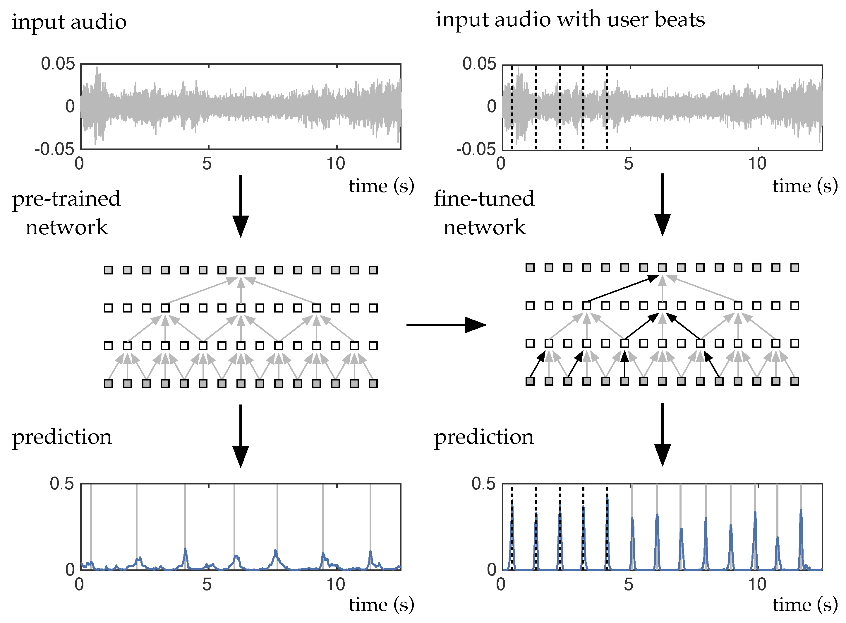
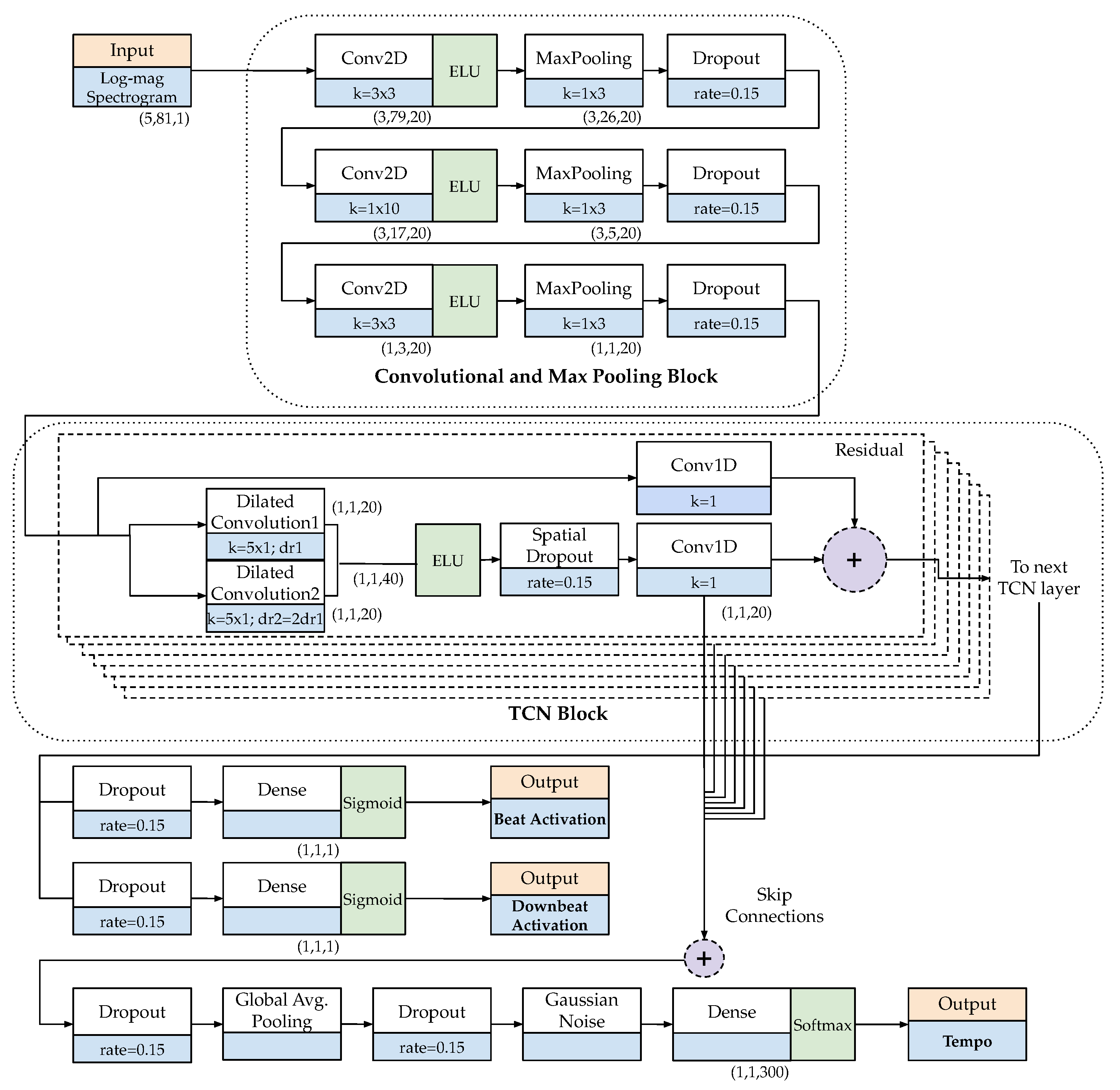
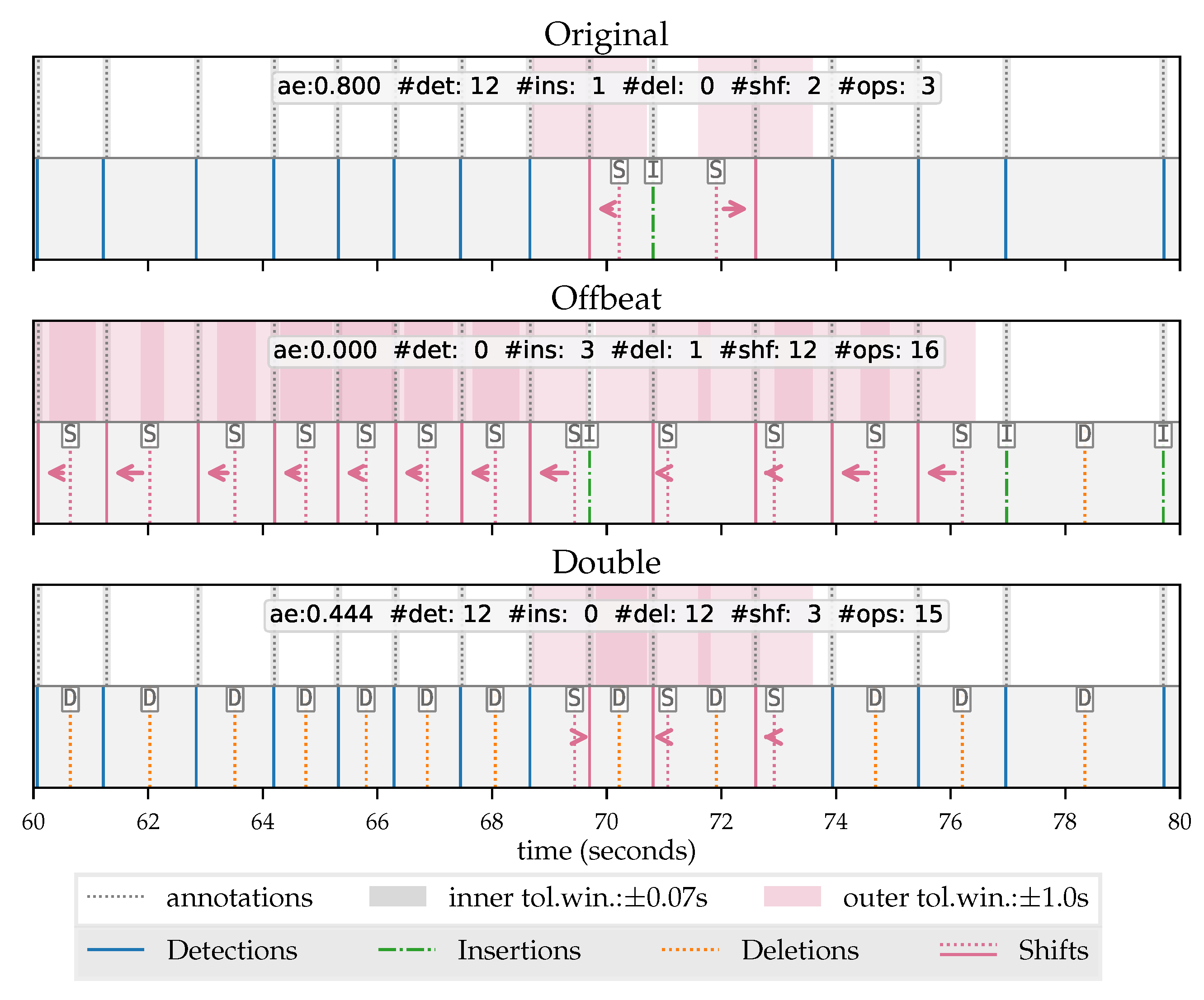
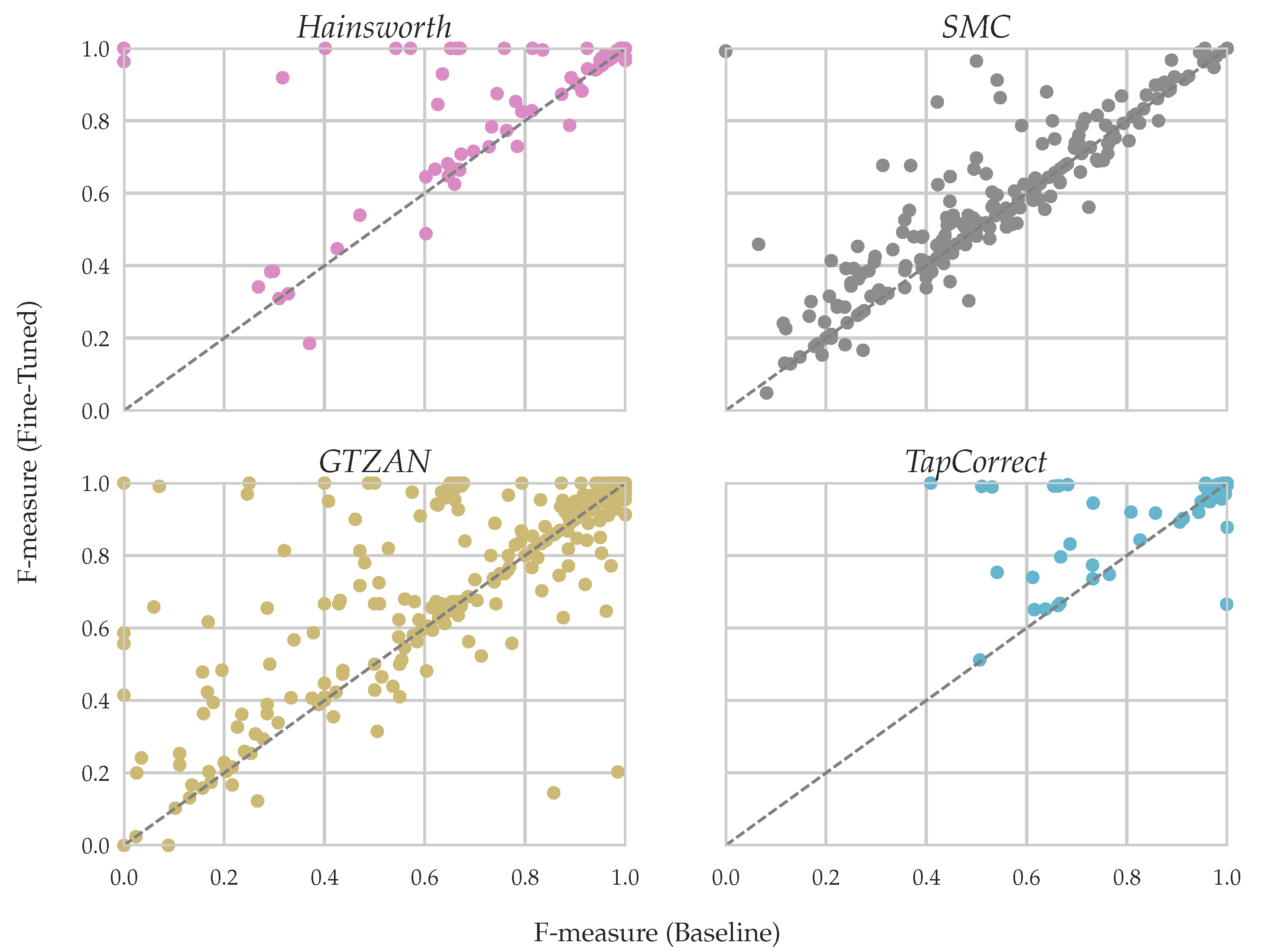
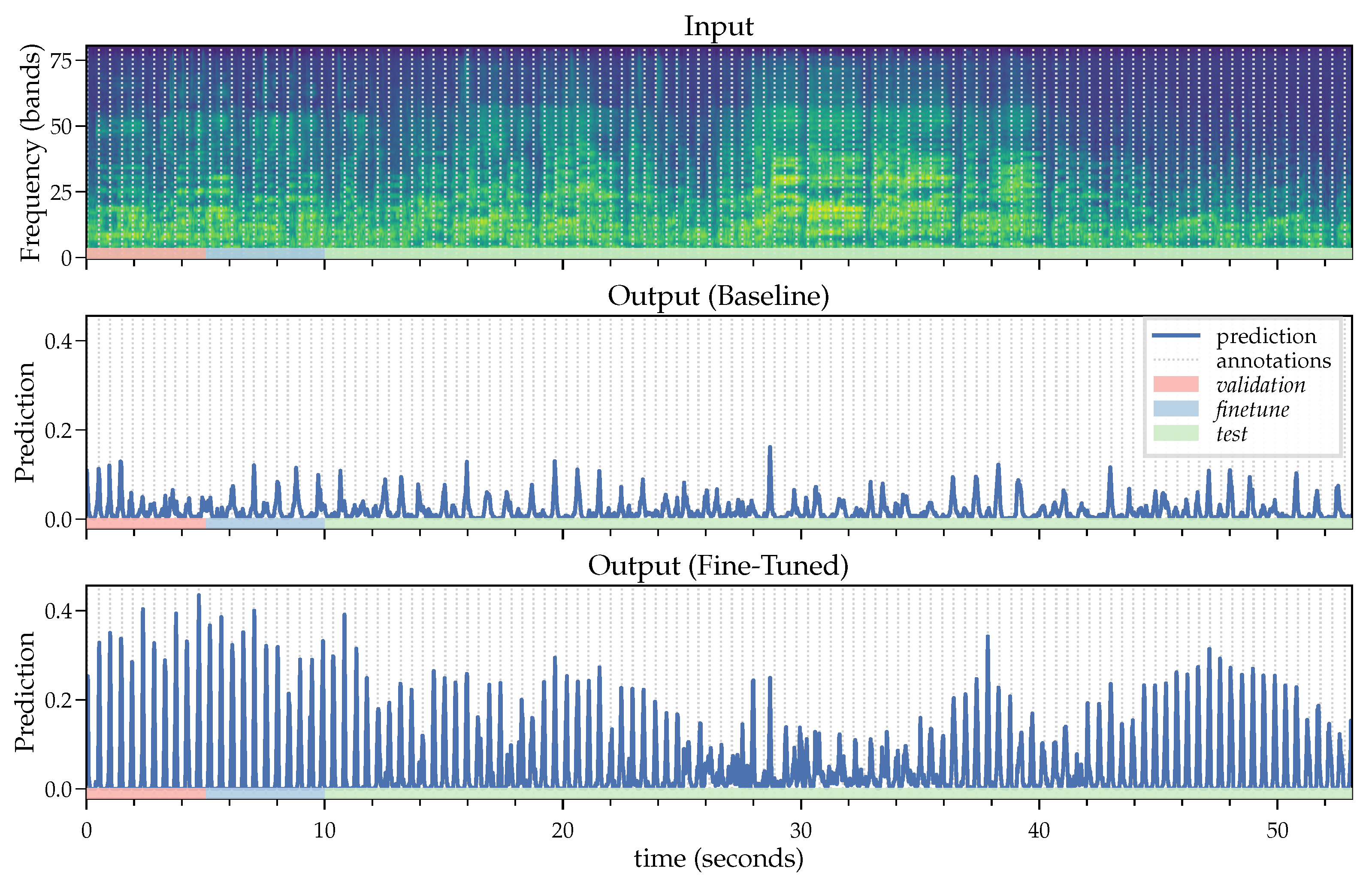
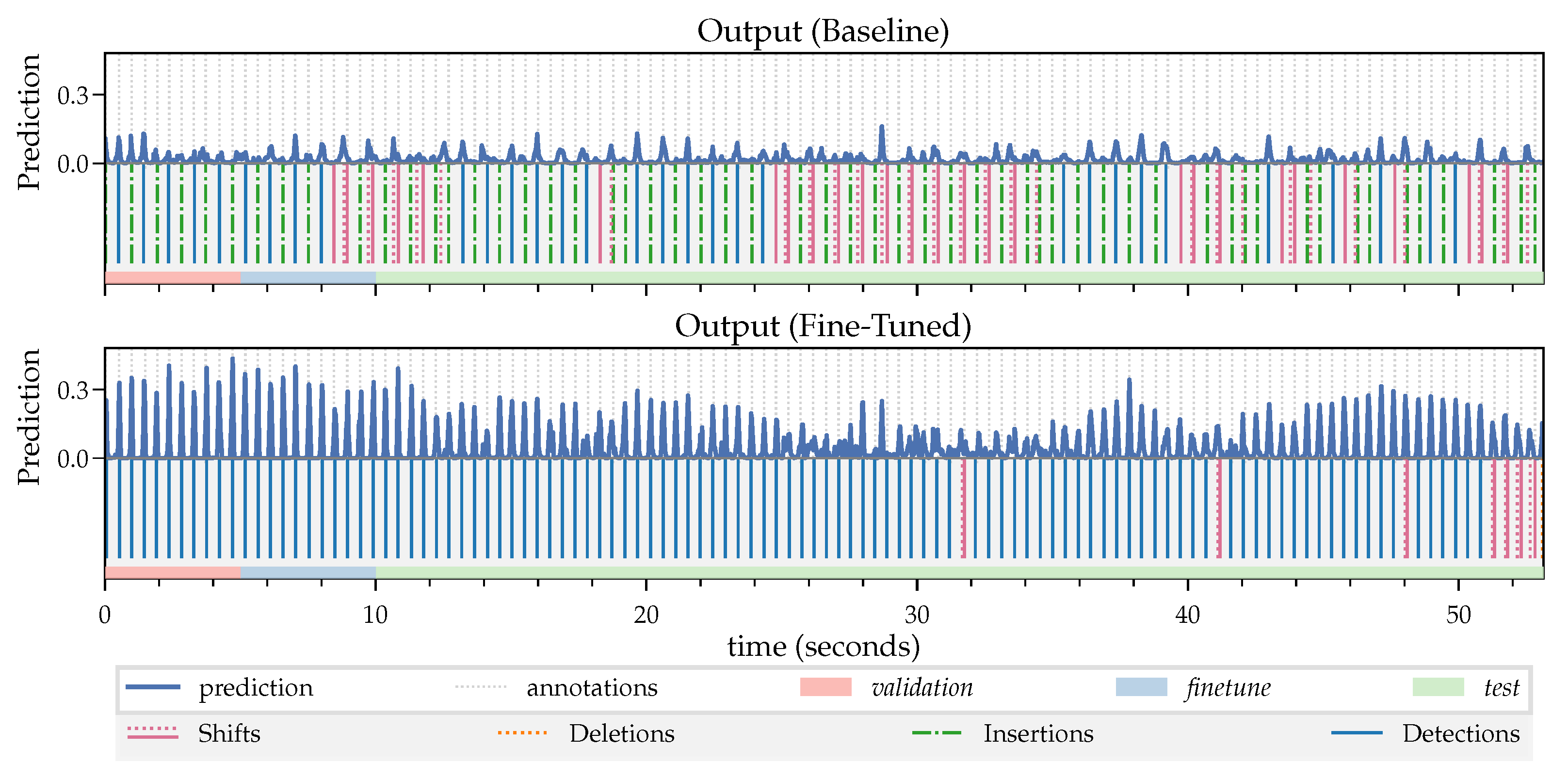
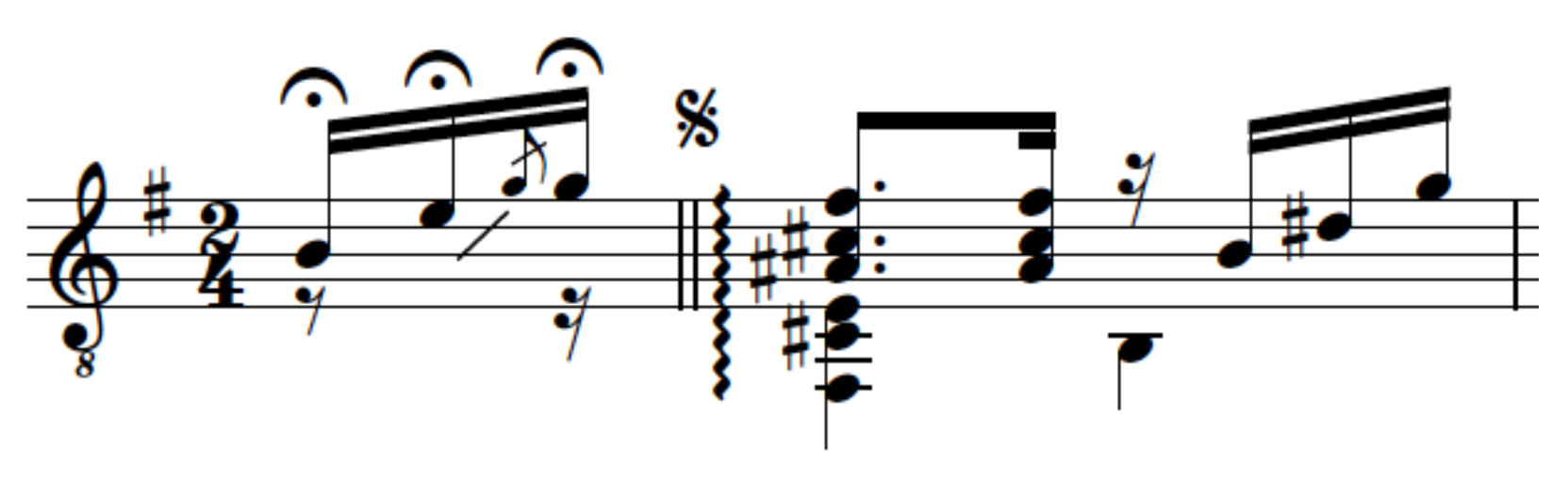
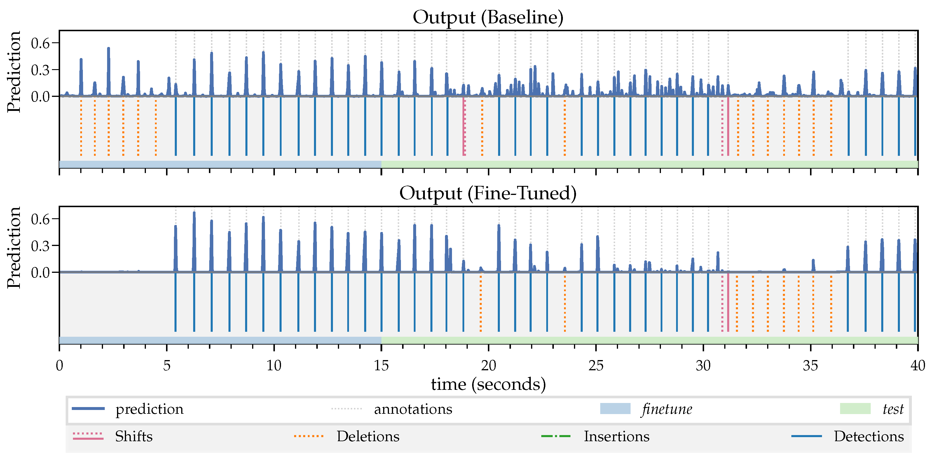
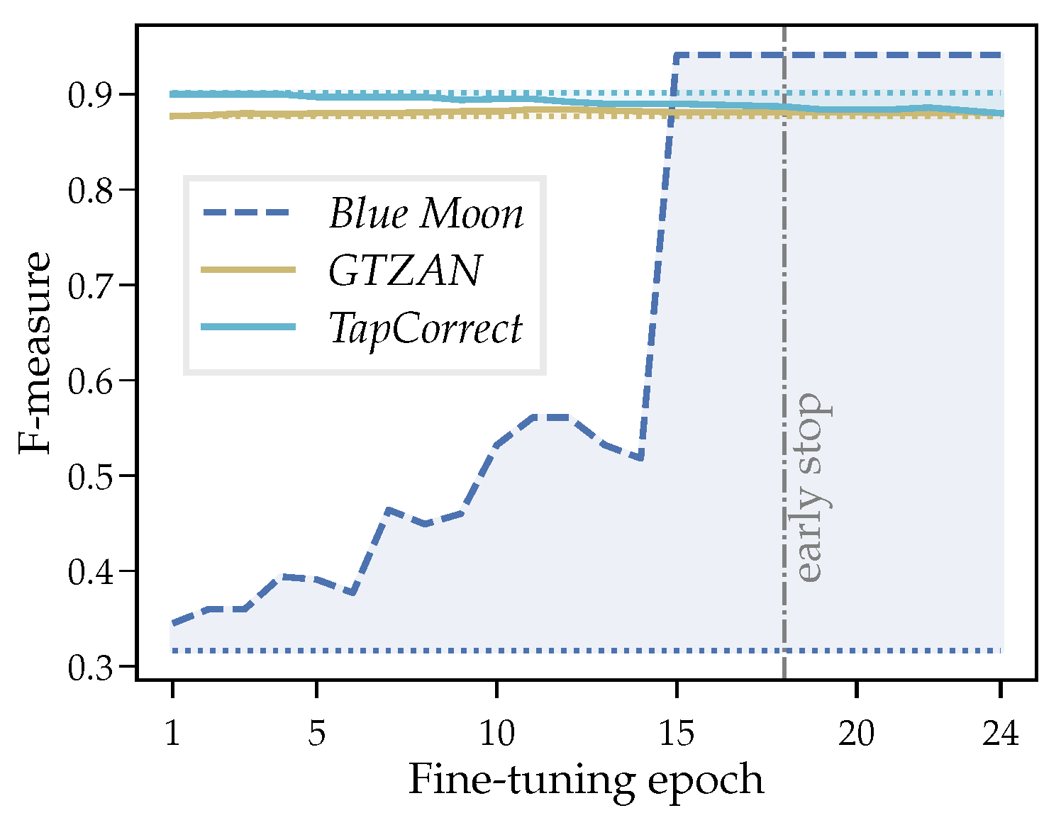
Table 1.
Overview of the datasets used for the evaluation.
| Dataset | # Files | Full Length | Mean File Length |
|---|---|---|---|
| Hainsworth | 222 | 3 h 19 m | 53 s |
| SMC | 217 | 2 h 25 m | 40 s |
| GTZAN | 999 | 8 h 18 m | 30 s |
| TapCorrect | 101 | 7 h 15 m | 4 m 18 s |
Table 2.
Mean F-measure scores across datasets for the baseline and fine-tuning approaches.
| Dataset | Baseline | Fine-Tuned |
|---|---|---|
| F-Measure | F-Measure | |
| Hainsworth | 0.899 | 0.945 |
| SMC | 0.551 | 0.589 |
| GTZAN | 0.879 | 0.917 |
| TapCorrect | 0.911 | 0.941 |
Table 3.
Global number of atomic edit operations: correct detections (#det), insertions (#ins), deletions (#del), shifts (#shf) and total edit operations (#ops) for the different test datasets.
Table 3.
Global number of atomic edit operations: correct detections (#det), insertions (#ins), deletions (#del), shifts (#shf) and total edit operations (#ops) for the different test datasets.
| Dataset | Model | #det | #ins | #del | #shf | #ops |
|---|---|---|---|---|---|---|
| Hainsworth | Baseline | 16,498 | 923 | 455 | 837 | 2215 |
| Fine-Tuned | 17,241 | 500 | 246 | 517 | 1263 | |
| SMC | Baseline | 4593 | 810 | 1337 | 2457 | 4604 |
| Fine-Tuned | 5028 | 670 | 1107 | 2162 | 3939 | |
| GTZAN | Baseline | 33,505 | 3348 | 1132 | 2235 | 6715 |
| Fine-Tuned | 35,403 | 1911 | 492 | 1774 | 4177 | |
| TapCorrect | Baseline | 35,072 | 3285 | 1622 | 910 | 5817 |
| Fine-Tuned | 36,659 | 2115 | 1236 | 493 | 3844 |
Table 4.
Annotation efficiency (ae), correct detections (#det) and insertions (#ins), deletions (#del), shifts (#shf) and total edit operations (#ops) for Blue Moon.
Table 4.
Annotation efficiency (ae), correct detections (#det) and insertions (#ins), deletions (#del), shifts (#shf) and total edit operations (#ops) for Blue Moon.
| ae | #det | #ins | #del | #shf | #ops | |
|---|---|---|---|---|---|---|
| Baseline | 0.272 | 31 | 56 | 0 | 27 | 83 |
| Fine-Tuned | 0.930 | 107 | 0 | 1 | 7 | 8 |
Table 5.
Annotation efficiency (ae), correct detections (#det) and insertions (#ins), deletions (#del), shifts (#shf) and total edit operations (#ops) for Choros №1.
Table 5.
Annotation efficiency (ae), correct detections (#det) and insertions (#ins), deletions (#del), shifts (#shf) and total edit operations (#ops) for Choros №1.
| ae | #det | #ins | #del | #shf | #ops | |
|---|---|---|---|---|---|---|
| Baseline | 0.555 | 207 | 0 | 69 | 97 | 166 |
| Fine-Tuned | 0.654 | 236 | 0 | 57 | 68 | 125 |
Publisher’s Note: MDPI stays neutral with regard to jurisdictional claims in published maps and institutional affiliations. |
© 2021 by the authors. Licensee MDPI, Basel, Switzerland. This article is an open access article distributed under the terms and conditions of the Creative Commons Attribution (CC BY) license (https://creativecommons.org/licenses/by/4.0/).
Share and Cite
MDPI and ACS Style
Pinto, A.S.; Böck, S.; Cardoso, J.S.; Davies, M.E.P. User-Driven Fine-Tuning for Beat Tracking. Electronics 2021, 10, 1518. https://doi.org/10.3390/electronics10131518
AMA Style
Pinto AS, Böck S, Cardoso JS, Davies MEP. User-Driven Fine-Tuning for Beat Tracking. Electronics. 2021; 10(13):1518. https://doi.org/10.3390/electronics10131518
Chicago/Turabian StylePinto, António S., Sebastian Böck, Jaime S. Cardoso, and Matthew E. P. Davies. 2021. "User-Driven Fine-Tuning for Beat Tracking" Electronics 10, no. 13: 1518. https://doi.org/10.3390/electronics10131518
Note that from the first issue of 2016, this journal uses article numbers instead of page numbers. See further details here.