Article

A Tightly-Coupled Positioning System of Online Calibrated RGB-D Camera and Wheel Odometry Based on SE(2) Plane Constraints

1
State Key Laboratory of Transducer Technology, Aerospace Information Research Institute, Chinese Academy of Sciences, Beijing 100190, China
2
University of Chinese Academy of Sciences, Beijing 100190, China
*
Author to whom correspondence should be addressed.
Electronics 2021, 10(8), 970; https://doi.org/10.3390/electronics10080970
Submission received: 3 March 2021 / Revised: 12 April 2021 / Accepted: 15 April 2021 / Published: 19 April 2021
(This article belongs to the Section Systems & Control Engineering)

Abstract

:
The emergence of Automated Guided Vehicle (AGV) has greatly increased the efficiency of the transportation industry, which put forward the urgent requirement for the accuracy and ease of use of 2D planar motion robot positioning. Multi-sensor fusion positioning has gradually become an important technical route to improve overall efficiency when dealing with AGV positioning. As a sensor directly acquiring depth, the RGB-D camera has received extensive attention in indoor positioning in recent years, while wheel odometry is the sensor that comes with most two-dimensional planar motion robots, and its parameters will not change over time. Both the RGB-D camera and the wheel odometry are commonly used sensors for indoor robot positioning, but the existing research on the fusion of RGB-D and wheel odometry is limited based on classic filtering algorithms; few fusion solutions based on optimization algorithm of them are available at present. To ensure the practicability and greatly improve the accuracy of RGB-D and odometry fusion positioning scheme, this paper proposed a tightly-coupled positioning scheme of online calibrated RGB-D camera and wheel odometry based on SE(2) plane constraints. Experiments have proved that the angle accuracy of the extrinsic parameter in the calibration part is less than 0.5 degrees, and the displacement of the extrinsic parameter reaches the millimeter level. The field-test positioning accuracy of the positioning system we proposed having reached centimeter-level on the dataset without pre-calibration, which is better than ORB-SLAM2 relying solely on RGB-D cameras. The experimental results verify the excellent performance of the frame in positioning accuracy and ease of use and prove that it can be a potential promising technical solution in the field of two-dimensional AGV positioning.

1. Introduction

With the vigorous development of industries such as autonomous driving and smart home, autonomous mobile robots have obtained increasing attention. In the process of unmanned vehicles performing tasks, accurate positioning information is a prerequisite for autonomous movement of robots, like AGV, vessels [1], UAV [2], and so on. In order to pick up this information, a variety of sensors are needed, whereas the measuring accuracy of different sensors differs from each other, such as vision [3,4], UWB [5], WiFi [6], and so on. The cost, usability, reliability, and positioning accuracy of the positioning system are determined by diverse sensor fusion schemes. It is necessary to make a suitable choice according to specific application conditions. Thus, selecting various sensors and fusing them to acquire accurate positioning information are very crucial [7]. According to the application characteristics of two-dimensional planar motion robots, two factors should be considered to solve its positioning problem: on the one hand, when the classic visual-inertial system is applied to solve the issue of two-dimensional planar motion, it will lead to unobservable scale information and poor accuracy [8]. On the other hand, the performance of some positioning methods based on motion sensors like inertial measurement units greatly depends on the performance of the sensors, which is closely related to the cost and installation quality of IMU [9] that greatly affects the usability and practicability of the fusion positioning system. Thus, the fusion of camera and wheel odometry is more suitable for solving the positioning problem of the planar motion AGV, which is only disturbed by the noise of the external environment, and the positioning results will not diverge over time [10]. In addition, most of the two-dimensional planar motion robots are equipped with wheel encoders, which means that using wheel odometry on mobile robots is a great choice.
As for access to obtain visual information, the RGB-D camera has become one of the mainstream sensors for visual positioning. According to the types of maps built, RGB-D SLAM can be divided into sparse maps and dense maps. Currently, most RGB-D SLAM algorithms are based on dense map building. KinectFusion [11] is the first real-time 3D reconstruction system based on the RGB-D camera. It uses ICP to estimate the pose by using the point cloud generated by depth images, but it requires GPU acceleration to maintain real-time performance. RTAB-MAP [12] is the most excellent RGB-D SLAM framework. It is a feature-based loop detection method with a memory management function and is mainly used for real-time image building based on appearance. The representative SLAM algorithm based on RGB-D camera sparse mapping is ORBSLAM2, which can realize the functions of map reuse, loop detection, and relocalization. Its main purpose is precise positioning. The biggest advantage of RGB-D camera is that it can directly obtain the depth value, which can be used to restore the scale of the map. Moreover, the function of real-time dense map building by RGB-D camera provides convenience for the robot’s subsequent navigation.
The fusion system of RGB-D and odometry has gradually attracted attention in the related field in recent years. Most of the attempts for the fusion of RGB-D and odometry are based on traditional filters like Kalman filter [13] and particle filter [14]. Although these works prove the advantages of the fusion of RGB-D and odometry, there are still some problems caused by using filtering algorithm for fusion positioning: compared with the fusion positioning based on optimization algorithm like vins-mono [15], the fusion positioning scheme based on filtering algorithm uses the output of wheel odometry to predict the state of the filter, and uses the visual measurement to update the state, which leads to the output of the whole fusion system being only related to the state of the adjacent previous moment, which means that all the historical information is not well used [16,17]. In addition, constraints for two-dimension planar motion robots is also an important algorithm that has importance for the fusion system but is hard to implement to the fusion scheme based on a traditional filter [18,19]: As shown in Figure 1, the displacement of the vertical axis (Z axis) and the rotation around the horizontal axis (X, Y axis) of the planar motion robot moving in the two-dimensional plane are very slightly, so that there has a planar motion constraint relationship, which can bring additional constraints to the fusion positioning scheme based on optimization algorithm to improve the positioning accuracy further.
In addition to the choice of core fusion algorithm, another unsolved problem of RGB-D and odometry fusion is that the fusion system needs to be calibrated offline in advance. The extrinsic parameter calibration method is a hot issue in visual positioning, and classic extrinsic parameter calibration methods used in the fusion of camera and wheel odometry [20,21,22] require external hardware equipment to get virtual feature points, so their practicality is greatly limited. DRE-SLAM [23] is a representative system based on the fusion of RGB-D camera and wheel odometry. The fusion system of RGB-D/odometry like DRE-SLAM is generally aiming at dynamic environments, but the extrinsic parameters between RGB-D camera and wheel odometry need to be calibrated offline. In addition, there is no restriction on the z-axis for the planar motion, which will cause an increasing disturbance on the z-axis.
For the purpose of improving the performance of fusion positioning system based on RGB-D/Odometry, and solving the practical problem of positioning in two-dimensional planar motion robot, this paper proposes a system based on extrinsic parameter calibration and tightly-coupled optimization of RGB-D camera and wheel odometry, for which extrinsic parameters are obtained according to online calibration, and positioning results based on SE(2) constraints to get better positioning performance. The fusion scheme realizes a high-accuracy, non-pre-calibration algorithm frame and solution by using the advantages of RGB-D camera/odometry and the unique characteristics of 2D planar motion robots like AGV. The main contributions of this work are:
  • A complete set of RGB-D and odometry fusion positioning technology scheme based on optimization algorithm with SE(2) planar constraints is proposed, which has better accuracy performance comparing with the fusion algorithm based on filter algorithm or the classic RGB-D SLAM frame.
  • Online calibration based on RGB-D depth information is supported, whose performance is better than the classic online calibration method. There is no need to calibrate the extrinsic parameters in advance offline, and the algorithm can be run directly in the case of unknown external parameters. Moreover, thanks to the depth information of RGB-D camera, no additional calibration scale information is needed.
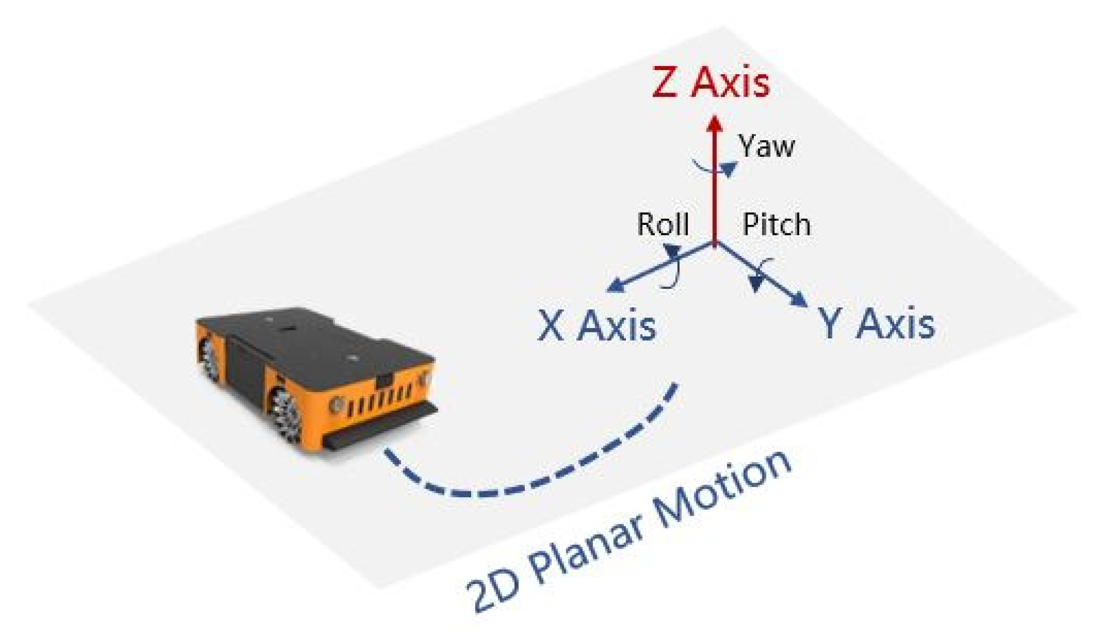
The remainder of the full text is structured as follows: Section 2 briefly introduces the relevant mathematical expressions used in this article. Section 3 illustrates the optimization algorithm based on SE(2) plane constraints and online extrinsic parameter calibration algorithm proposed in this article along with the tightly-coupled positioning architecture. Section 4 describes the experimental setup and the achieved results of the algorithm; Section 5 is the summary.

2. Preparation

First of all, the symbols used throughout this paper are briefly defined. The system consists of multiple coordinate systems, and the right-hand rule is chosen:
{ W } : World coordinate system;
{ O } : Wheel odometry coordinate system;
{ C } : Camera coordinate system.
Throughout this manuscript, we use T B A to express the pose transformation from the coordinate system { B } to the coordinate system { A } . Considering the time parameters, A t represents the coordinate system { A } at time t. R B A and p B A represent rotation and translation, respectively. q B A = [ q B w A , q B x A , q B y A , q B z A ] T is a unit quaternion that can also represent rotation from { B } to { A } . The multiplication of quaternions can be expressed as
q 1 q 2 = L ( q 1 ) q 2 = q 1 R ( q 2 )
where
L ( q ) = [ q w q z q y q x q z q w q x q y q y q x q w q z q x q y q z q w ]
R ( q ) = q w q z q y q x q z q w q x q y q y q x q w q z q x q y q z q w
The pose between two coordinates can be expressed as Lie group S E ( 3 ) and Lie algebra s e ( 3 ) [24]
S E ( 3 ) = T = R p 0 T 1 R 4 × 4 | R S O ( 3 ) , p R 3
s e ( 3 ) = ξ = ρ ϕ R 6 , ρ R 3 , ϕ s o ( 3 ) , ξ = ϕ ρ 0 T 0 R 4 × 4
where S O ( 3 ) is special orthogonal group and S E ( 3 ) is special Euclidean groups, and the group is an algebraic structure of a set plus an operation. As indicated by s e ( 3 ) , it has six dimensions, which can be specifically expressed as ξ = [ w 1 , w 2 , w 3 , v 1 , v 2 , v 3 ] T . The first three ρ = [ w 1 , w 2 , w 3 ] T represent the angle of rotation around the x-, y-, and z-axis, and the latter three ϕ = [ v 1 , v 2 , v 3 ] T represent the displacement in the x-, y-, and z-axis plane. In addition, the relationship between S E ( 3 ) and s e ( 3 ) can be expressed as
T = exp ( ξ ) = E x p ( ξ )
ξ = log ( T ) = L o g ( T )
In the ideal case, the motion of a planar robot is effective only on three dimensions s e ( 2 ) = [ w 3 , v 1 , v 2 ] T [25]. However, the wheeled robots may suffer from rough terrains, load changes, and shaking. The transformation between s e ( 2 ) and s e ( 3 ) can be expressed by the following formula:
s e ( 3 ) = f ( s e ( 2 ) ) = [ 0 , 0 , w 3 , v 1 , v 2 , 0 ] T
s e ( 2 ) = f 1 ( s e ( 3 ) ) = [ w 3 , v 1 , v 2 ] T

3. Fusion Algorithm

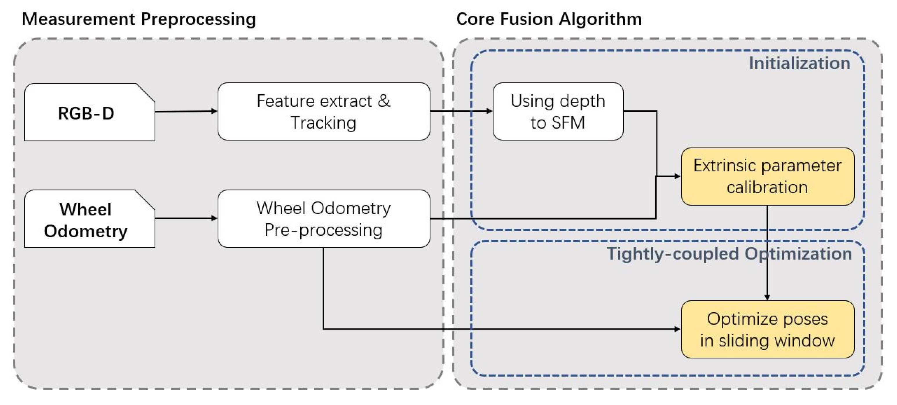
3.1. Overview of Algorithm Framework

The framework of the entire fusion algorithm is shown in Figure 2. The first part is measurement preprocessing, the data of wheel odometry and RGB-D camera are taken as input and processed, and their results are sent to the core fusion algorithm part. The core fusion algorithm part is mainly divided into two parts: one is initialization, the other is tightly-coupled optimization. Initialization is only performed at the beginning of the program. After obtaining extrinsic parameters, it is used as the input for tightly-coupled positioning and optimized together with the robot pose.
The brief introduction of each part is as follows:
Measurement preprocessing: This process first collects data from RGB-D and wheel odometry. The preprocessing of image data is to extract feature points [26] and use optical flow algorithm [27] for tracking, while that of wheel odometry data are to carry out pre-integration and covariance transmission on the collected angle and speed information [28]. Because this part adopts the existing conventional algorithm, it will not be introduced in more detail later considering the space limitation:
Initialization: The first step in this process is to know the relative poses of the wheel odometry and the RGB-D camera between two consecutive images. The relative pose of the wheel odometry has been obtained through the data preprocessing part. In addition, since the image has depth information, we can recover the real scale map and use PnP [27] to recover the image pose. Afterwards, the extrinsic parameters are calibrated using analytical solutions and optimized forms according to the relative poses of the two.
Tightly-coupled optimization: This process maintains a sliding window that contains quantitative keyframes. Whenever a new keyframe comes, the oldest keyframe in the sliding window will be eliminated. The goal of optimization in the window is the pose of the keyframe and the extrinsic parameters and the inverse depth of the feature points. This paper uses the nonlinear least-squares method to optimize four objective functions, prior errors, reprojection errors, odometry errors [15,28], and plane SE(2) errors.
The core fusion algorithm is the main innovation of this paper, which introduces the depth of the RGB-D camera for online extrinsic parameter calibration and uses SE(2) planar constraints for tightly-coupled positioning, and these parts are highlighted in the algorithm framework diagram. The following is a detailed introduction to the two parts of core fusion algorithm.

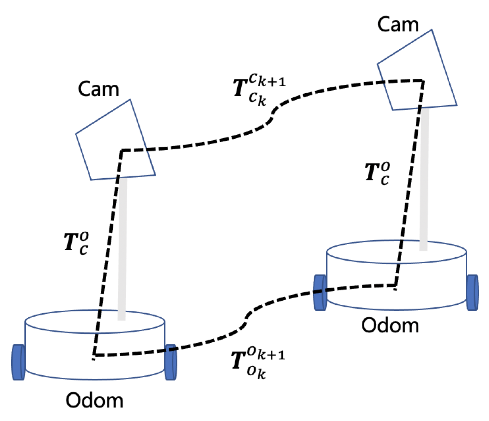
3.2. Initialization Algorithm

Classical parameter calibration initialization methods often use analytical solutions to solve the extrinsic parameters and scale between the camera and the wheel odometry [29]. However, fusion positioning systems that use the classic calibration method often require the additional calculation of scale information, which is more likely to cause errors. Furthermore, the classic calibration methods require the fusion system to carry out a series of offline calibration processing according to the established operation process before application, which increases the inconvenience of the system. Therefore, the fusion scheme we proposed reduces the solution of scale and adds the process of nonlinear optimization, which can realize the online extrinsic parameter calibration between the RGB-D camera and the wheel odometry.
The extrinsic calibration parameters are defined as follows:
T c o = ( q c o , p c o ) = ( q c x o , q c y o , q c z o , q c w o , p c x o , p c y o , p c z o ) ,
where q c o and p c o represent the rotation and translation from camera to wheel odometry. Although there are eight extrinsic parameters, The displacement of the extrinsic parameters in the z-axis direction p c z o has no effect on the system during the experiment [28], so the error of the z-axis does not need to be taken into consideration.
The initialization algorithm to support online extrinsic parameter calibration in this system is divided into three steps, as Figure 3. Different from the system that requires scale information to complete extrinsic parameter calibration, the initialization algorithm in this paper directly collects the feature points extracted from the acquired image as calibration information. Then, it combines the depth information obtained by RGB-D to back-project the feature points to get real three-dimensional landmarks. PnP and triangulation [27] are finally used to solve the relative pose, which avoids solving scale and realizes the online extrinsic parameter calibration of the scale without the calibration board. Therefore, the scale information does not need to be solved according to this, which reduces the variables that need to be calculated. Eventually, the initial calibration extrinsic parameters are obtained and fine-tuned through nonlinear optimization in the sliding window optimization part. The calculation part of the analytical solution is shown below.
As the Figure 4 shows, the hand-eye calibration problem can be expressed as
T o k o k + 1 T c o = T c o T c k c k + 1
where T o k o k + 1 is the relative pose between time k and k + 1 in the wheel odometry coordinate, and T c k c k + 1 is the relative pose between time k and k + 1 in the camera coordinate. The above expression can also be written in terms of rotation quaternion and displacement:
q o k o k + 1 q c o = q c o q c k c k + 1
( R o k o k + 1 I ) p c o = R c o p c k c k + 1 p o k o k + 1 ,
where I is the identity matrix, q o k o k + 1 and p o k o k + 1 the relative rotation and translation of the wheel odometry between time k and k + 1 , q c k c k + 1 and p c k c k + 1 the relative rotation and translation of the camera between the time k and k + 1 . The calculation process of the extrinsic parameters is similar to [29]. The solution process is shown in Figure 3.
First of all, we solve the pitch and roll angle of the rotation extrinsic parameters, and the formula is as Equation (14):
q y x = arg min q y x M q y x , M = L ( q o m o m + 1 ) R ( q c m c m + 1 ) L ( q o 0 o 1 ) R ( q c 0 c 1 ) , m [ 0 , n ] ,
where q c o = q z ( γ ) q y ( β ) q x ( α ) , q z ( γ ) , q y ( β ) and q x ( α ) correspond to yaw, pitch, and roll quaternion, respectively, and q y x = q y ( β ) q x ( α ) . γ , β , α are yaw, pitch, and roll angles. The size of n is the same as the number of keyframes for the sliding window in backend optimization. In addition, then, we solve the other parameters:
m = arg min m G m + w ,
where
G = J m K m J 0 K 0 , m = p c x o p c y o cos γ sin γ w = p m p 0 , m [ 0 , n ] ,
and
cos ϕ k 1 sin ϕ k sin ϕ k cos ϕ k 1 J k p c x o p c y o p k 1 p k 2 p k 2 p k 1 K k cos γ sin γ + p o k x o k + 1 p o k y o k + 1 p k = 0 ,
In Equation (17), ϕ k represents the angle of rotation q o k o k + 1 around the z-axis. p k 1 and p k 2 represent the first two terms of R ( q y x ) p c k c k + 1 . In addition, the γ is the yaw angle of the rotation extrinsic parameters and p c x o , p c y o are the first two dimensions of the extrinsic translation. p o k x o k + 1 and p o k y o k + 1 denote the first two elements of the vector p o k o k + 1 . Finally, we can refine the results though the nonlinear optimization as Equation (18):
q c o , p c o = argmin q c o , p c o k = 0 m R o k o k + 1 I p c o R c o p c k c k + 1 + p o k o k + 1 ,
In summary, the initial extrinsic parameters can be found in the form of analytical solutions, which means that the calibration process is completed online.

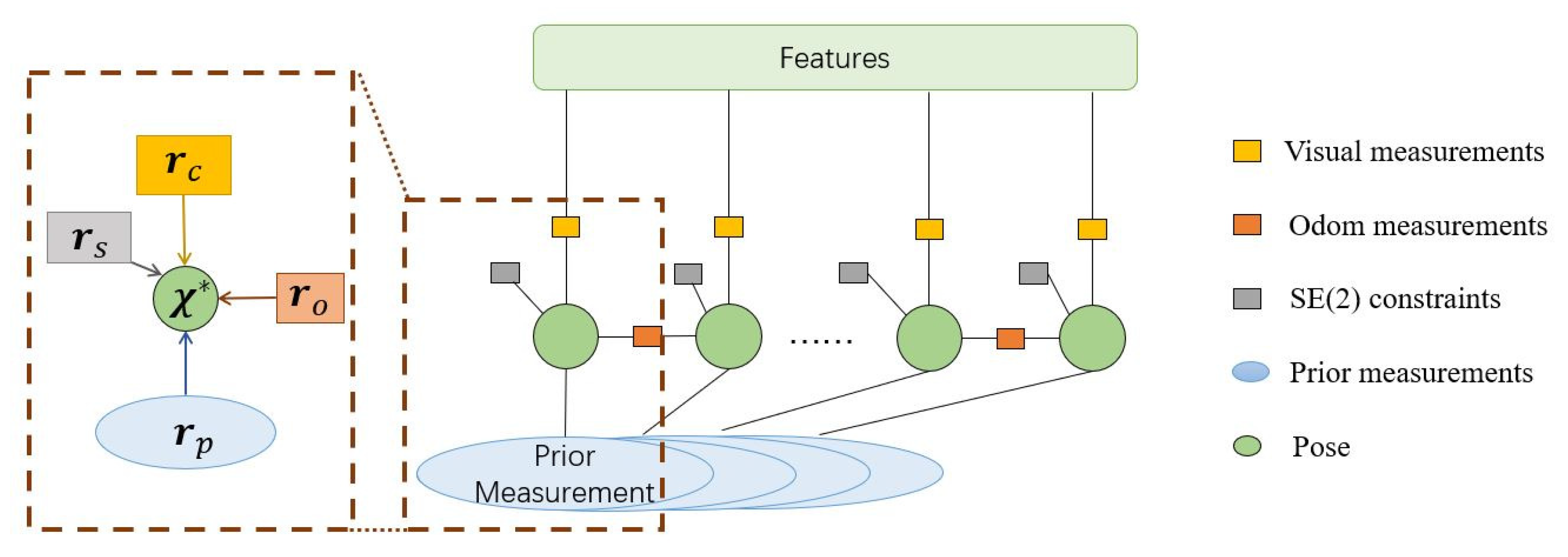
3.3. Tightly-Coupled Optimization Based on SE (2) Plane Constraints

For a robot moving in a two-dimensional plane, its posture mainly depends on the displacement in the x- and y-planes and the angle of rotation around the z-axis. Nevertheless, the optimization goal in the actual process is three-dimensional rotation and displacement. Taking the features of planar motion into account, this paper proposes the SE(2) constraints on SE(3), which reduce the displacement of the posture in the z-axis direction and the disturbance of the angle around the x- and y-axes. As one of the optimization objectives, SE(2) constraints along with other optimization objectives constitute the tightly-coupled optimization between the RGB-D camera and the wheel odometry, thus improving the positioning accuracy and robustness by introducing constraint conditions compared to the directly-coupled scheme of RGB-D and odometry. The specific process of tightly-coupled optimization is as follows.
The variables that need to be optimized in this process are
Ø = x 1 , x 2 , , x n , R c o , p c o , λ 1 , λ 2 , , λ m ,
x k = R o k w , p o k w = T o k w ,
In Equation (20), x k is the pose state of the wheel odometry under the k-th keyframe, including the position of the wheel odometry in the world coordinate system p o k w and the rotation of the wheel odometry relative to the world coordinate system R o k w .We use the T o k w as robot pose. n represents the number of keyframes in the window, while m represents the number of feature points observed in the window. λ k is the inverse depth of the feature point k in the camera coordinate system of the first observed keyframe. In this process, four objective items need to be optimized. As shown in Figure 5,
Ø = arg min Ø { | r p | 2 + ρ ( | r c | 2 ) + | r o | 2 + | r s | 2 } ,
The constraint relationship shown in Figure 5, where r p is a prior constraint, r c is the camera reprojection error constraint, r o the odometry constraint, and r s the plane-based SE(2) constraint. ρ is the robust kernel [30], and we used the Huber kernel in this article
ρ ( r ) = 1 , r 1 2 r 1 , r < 1
The specific forms of r p and r c are similar to [15], whereas r o is based on the characteristics of planar motion. The processing of each items in the optimization function is introduced as follows:
r c is the camera reprojection error constraint, expressed as Equation (23):
r c = P j l P ^ j l | | P ^ j l | | ,
P j l = u j l , v j l , 1 ,
P ^ j l = R o c R w o j R o i w R c o 1 λ l P i l + p c o + p o i w p o j w p c o ,
where P i l and P j l are the normalized coordinates that is observed in the frame i and frame j. u j l and v j l are the coordinates of landmark l in the image j. By the chain rule, the Jacobian can be derived as [15].
r o is the odometry constraint, which can be modeled as
r o = T o k w 1 T o k + 1 w T o k o k + 1 ,
It connects two consecutive keyframes T o k + 1 w and T o k w in the sliding window, and T o k o k + 1 is the pre-integration between the two consecutive keyframes.
We used SE(3) to express the pose. It has six dimensions, and sometimes the three dimensions can express the planar motion but the z-axis is affected when the car is bumping, and the value is not zero. Another reason is that, when the plane robot is moving in a plane, there may be a disturbance in the z-axis, so the SE(2) plane constraints are added. First of all, the pose is projected to SE(2) and then restored, bringing to SE(3) [19]
ζ = f 1 L o g T o k w ,
T ¯ o k w = E x p f ζ ,
T ¯ o k w is the constraint term, and the form of r s is
r s = T ¯ o k w 1 T o k w ,
The value of the covariance matrix of this constraint can be expressed as
Ω = d i a g δ , δ , 1 σ w 2 , 1 σ v 2 , 1 σ v 2 , δ ,
where δ represents a particularly small value close to 0, and σ w 2 , σ v 2 are the covariance of angular velocity and linear velocity. Finally, the derivative of r s is
r s E x p δ ξ o k ¯ o k = T o k w ¯ 1 T o k w E x p δ ξ o k ,
( T ¯ o k w ) 1 T o k w E x p δ ξ o k ¯ o k = T ¯ o k w 1 T o k w E x p δ ξ o k ,
δ ξ o k ¯ o k = δ ξ o k ,
Thus, the Jacobian matrix at time k is
J k k = I ,
Thus far, the items in the optimization function have been processed, and we have completed the tightly coupled fusion algorithm.

4. Simulation and Real-Site Experiment Results

In order to fully verify the comprehensive performance of the fusion positioning system proposed in this paper, several simulation and real-site experiments were conducted. Simulations are performed by using the dataset from DRE-SLAM Datasets, which not only contains the data of RGB-D camera and wheel odometry, but also contains the truth value of positioning. Real-site experiments were carried out in the garden in Aerospace Information Research Institute (Beijing) with a real 2D navigation AGV.

4.1. Simulations and Comparisons

To prove the effectiveness of our approach, three parts of experiments are designed and conducted to testify the accuracy of extrinsic parameter calibration and the positioning accuracy, respectively:
1.
Calibration accuracy test of extrinsic parameters;
2.
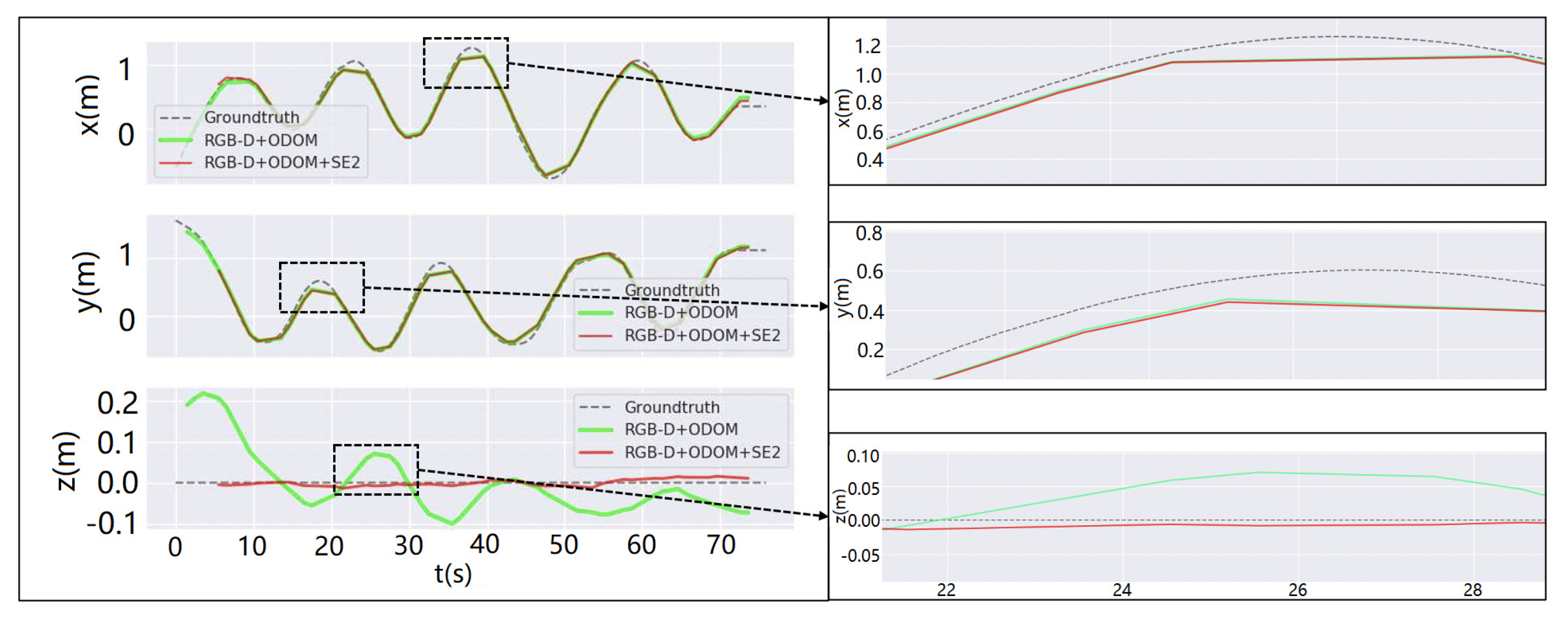
Positioning accuracy comparison of the fusion positioning system with and without the plane SE(2) constraints;
3.
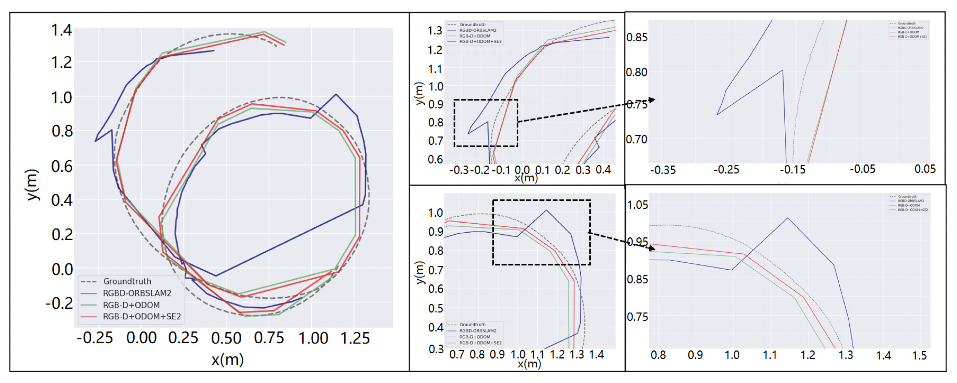
Positioning accuracy comparison of the fusion positioning system we proposed and RGB-D ORB-SLAM2.
The method in this paper is built under the framework of ROS [31] and solved by Ceres [32]. The simulations run on a laptop with a CPU configuration of Intel Core i7-8565U, 1.8 GHz, and 8 GB memory.

4.1.1. Calibration Accuracy Test of Extrinsic Parameters

The displacement of the extrinsic parameters in the z-axis direction has no effect on the system during the experiment, so the error of the z-axis does not need to be taken into consideration and will be directly set to zero. In this process, the true value results of the extrinsic parameters in DRE-SLAM datasets are
T t r u t h = 0.0 0.276 0.961 0.124 1.0 0.0 0.0 0.1 0.0 0.961 0.276 0.0 0.0 0.0 0.0 1.0
In order to make the errors in the experimental results more clearly, we convert the rotation matrix into the form of Euler angles, as T t r u t h ( r o l l = 1 . 2911 , p i t c h = 0 , y a w = 1 . 5708 , t x = 0.124 m , t y = 0.1 m ) . The results of the extrinsic parameters from the analytic solution that is used in the initialization are as follows:
T i n i t i a l = 0.0262 0.1225 0.9921 0.096 0.9987 0.0459 0.0207 0.201 0.043 0.9914 0.1236 0.0 0 0 0 1
The results after the optimization are
T f i n a l = 0.012 0.074 0.997 0.126 0.9999 0.0025 0.012 0.105 0.0034 0.997 0.074 0.0 0.0 0.0 0.0 1.0
The extrinsic parameters matrix can be transformed into Euler angles. The initial result is T i n i t i a l ( r o l l = 1 . 6948 , p i t c h = 0 . 043 , y a w = 1 . 5971 , t x = 0.096 m , t y = 0.201 m ) and the final result is T f i n a l ( r o l l = 1 . 645 , p i t c h = 0 . 0034 , y a w = 1 . 5588 , t x = 0.126 m , t y = 0.105 m ) . It can be seen from the final results that the maximum error of the angle is the roll angle with a degree of 0.35, and the position error does not exceed 1 cm. The experiment results show the better performance compared to the other online extrinsic calibration methods like [22], for which the maximum error of rotation in the extrinsic parameters is 3.1 degrees of roll Angle and 3 cm for translation.

4.1.2. Positioning Accuracy Comparison

To compare this paper with the state-of-the-art visual estimation methods, we also conducted tests of the open-source framework ORB-SLAM2 on the same datasets. RGB-D ORBSLAM2 uses sparse feature points and nonlinear optimization to improve positioning accuracy. Our method also uses sparse feature points, and the goal is to improve positioning accuracy.
Evo [33] tool was used to compare and visualize the results. Corresponding poses are directly compared between estimates, and references gave a pose relation. The absolute pose error of evo is often used as trajectory error. Then, statistics for the whole trajectory are calculated. Thus, we used it as the criterion. The calculation formula can be expressed as RESE (Root Mean Squard Error)
R M S E = 1 n k = 1 n ( p k , i e s t i m a t o r p k , i t r u t h ) 2 , i ( x , y , z )
where n is the total number of poses. The RMSE is used to evaluate the absolute error in evo, and our results can be expressed as follows.

4.1.3. Comparison of Results with SE(2) Plane Constraints

In the process of optimization, an error term based on SE(2) constraints is proposed. The error is mainly based on planar motion robots, which have a slight disturbance in the z-axis but do not bring a bigger drift. As shown in Figure 6, the results illustrate a displacement comparison on each axis with and without SE(2) constraints of a random motion of AGV, where the gray dashed line represents the true value of displacement, the green line represents the result without SE(2) constraints, and the red line represents the result with SE(2) constraints. It can be seen that the displacement in a period of random motion mapped on the z-axis is very small, but the classic fusion algorithm without SE(2) constraints obviously cannot take advantage of the motion feature, resulting in a large deviation of the calculation results. The fusion algorithm with SE(2) constraints improves the positioning accuracy, which is of great support to improve the performance of the final fusion positioning system. In addition, we can also see from the zoomed-in area that the SE(2) constraint greatly improves the accuracy of the z-axis direction and thus improves the overall positioning progress.

4.1.4. Comprehensive Comparison of Positioning Accuracy
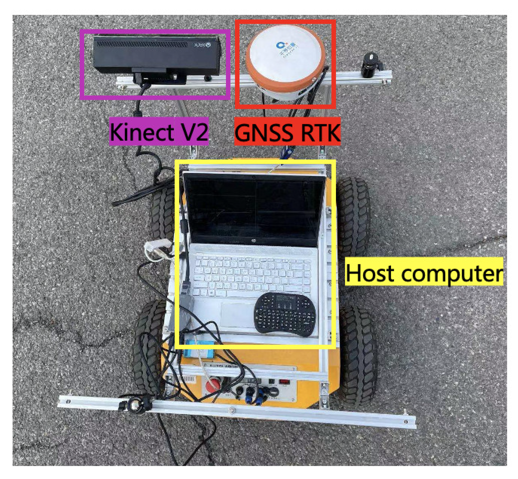
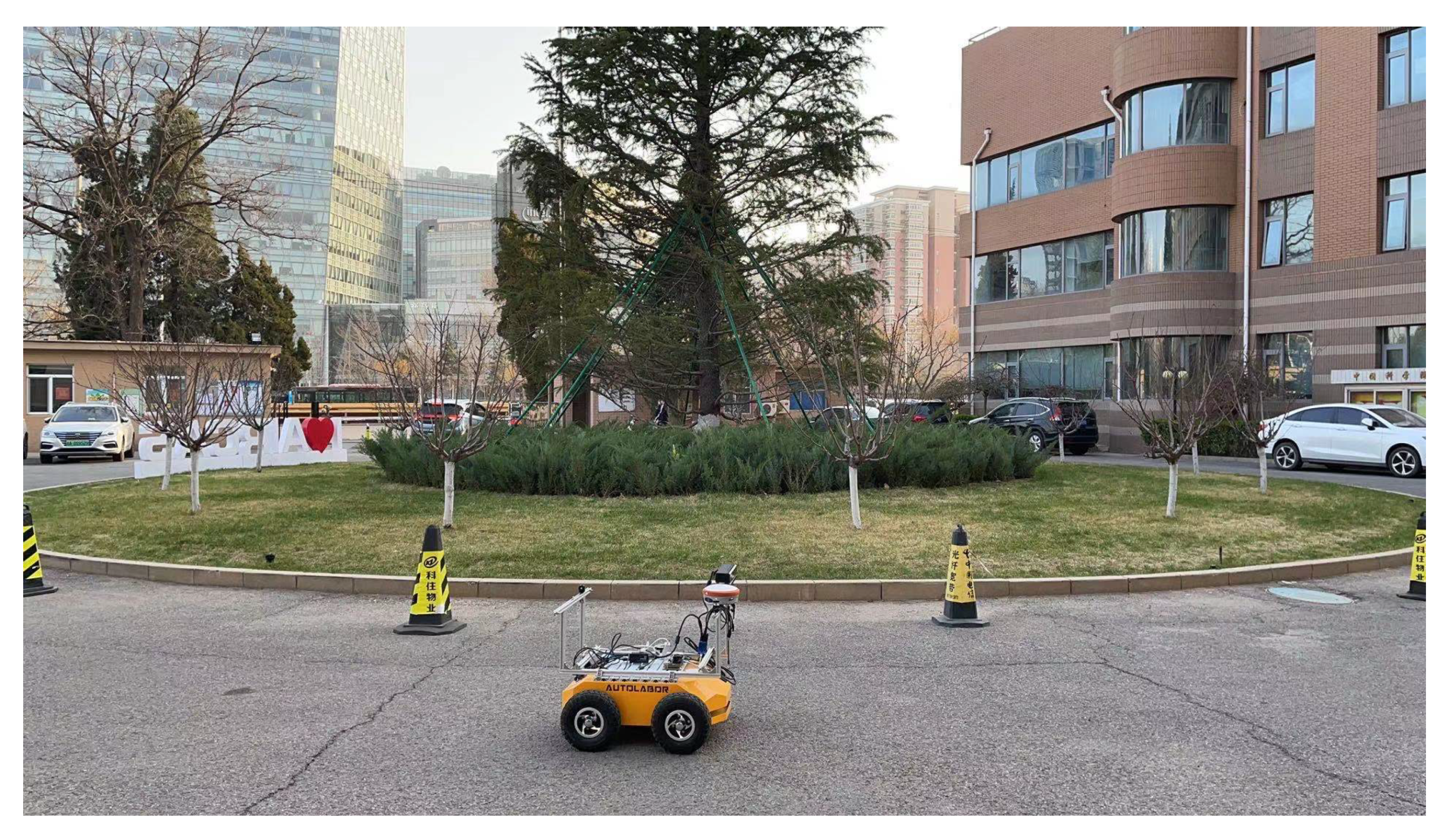
In order to comprehensively verify the positioning performance of the proposed system, a comparison experiment was conducted to compare the positioning accuracy of the classic ORB-SLAM framework with RGB-D camera [34] and the proposed fusion positioning system (with and without SE(2) constraints) based on DRE-SLAM dataset. EVO tool is used to perform accuracy conversion.
Figure 7 shows a segment of positioning results, where the gray dashed line is the ground truth, the blue line is the result of ORB-SLAM2 positioning with RGB-D camera, the green line and red line are the results of the proposed fusion positioning system with and without SE(2) constraints, respectively. The right view of the image is the enlarged left view of Figure 7, where it can be seen clearly that the random jitter of the proposed fusion positioning system is smaller and the positioning accuracy is much better than that of the ORB-SLAM2 framework, no matter whether the system has or does not have the SE(2) constraint. The introduction of the SE(2) constraint further improves the positioning accuracy.
To reflect the improvement of positioning accuracy of the system, the average positioning accuracy (RMSE) results of different fusion frameworks are shown and compared in Table 1 and Table 2. It can be seen from the table that, compared with ORB-SLAM2, the accuracy of the proposed fusion positioning system has been improved by 22.46% on average. After the SE(2) constraints are added, the positioning accuracy is improved by 17.86% further on average. Compared with the fusion scheme of RGB-D and odometry based on traditional filtering algorithms, the fusion scheme we proposed can improve the average positioning accuracy by more than two times without offline calibration. In addition, the scheme in this paper achieves centimeter-level accuracy, which means that it can meet the requirements of most two-dimensional AGV applications.

4.2. Experiments

In order to verify the accuracy and practicability of the algorithm, we deployed and verified the algorithm on a real robot, as is shown in Figure 8. The platform for the experiment is a differential robot called the Autolabor Pro1, which has a wheeled encoder with an accuracy of 400 lines. The front of the robot is mounted with a Kinect V2, which is an RGB-D camera. The ground truth of the robot is collected by a GNSS RTK with positioning accuracy that can reach 2 cm. We use ROS to collect the topics of each sensor and store them in a bag. Our algorithm can be run in real-time under the recorded bag, and the total processing time for each frame is no more than 60 ms.
In order to better collect truth data, we conducted experiments in a relatively empty place, as shown in Figure 9. During the experiment, we made the robot make a circle around the flower bed. Figure 10 shows the trajectory between the results of our algorithm and the ground truth. Both the horizontal axis and the vertical axis show the position. The black dashed line is the RTK result, and the red line is the results of our algorithm. It is seen that the trajectories are close.
The relative position error is used to evaluate the positioning result between the algorithm and the RTK result, and the formula is shown as follows:
R P E t r a n s = 1 4 k = 1 4 i = x , y , z ( p k , i e s t i m a t o r p k , i t r u t h ) 2
In order to better measure the error, we draw the RPE result between our positioning results and the truth value. As shown in Figure 11, the vertical axis shows the RPE error, and the horizontal axis shows the number of comparisons. It can be seen that the maximum error is no more than 0.1 m.
Whereas many positioning methods using RGB-D cameras are based on dense maps, our method uses sparse maps and can be used outdoors. Therefore, we make a comparison with the positioning method of the RGB-D camera and wheel odometry based on sparse feature points. The method in [13] fuse the RGB-D camera and wheel odometry based on the filter method and use their robots to acquire the results. The average error of our positioning results was 0.0297 m, which is better than the RMSE of 0.153 m in [13].

5. Conclusions

This paper proposes a tightly-coupled positioning system of online calibrated RGB-D camera and wheel odometry based on SE(2) plane constraints. Compared with the existing fusion positioning systems of RGB-D and odometry, the system we proposed innovatively introduces SE(2) plane constraints into the tightly-coupled optimization framework, which leads to the great positioning accuracy, and uses the depth information obtained from RGB-D camera to realize the online calibration, which leads to the better usability. Experiment results proved that the angle and position calibration accuracy reaches the 0.5 degree millimeter level with online calibration, respectively, and the positioning accuracy of the fusion positioning system achieves the centimeter level, which means that, when ORBSLAM2 is not supported, our algorithm still provides service. The fusion positioning system proposed in this paper not only satisfies the need for online extrinsic parameter calibration between the RGB-D camera and the wheel odometry but also greatly improves the positioning accuracy. To make the fusion system of the RGB-D camera and the wheel odometry a promising candidate in the future two-dimensional AGV positioning applications, loop closing will be introduced into the framework to achieve better positioning accuracy in large scenes in later work.

Author Contributions

Conceptualization, L.Z.; methodology, L.Z.; software, L.Z.; validation, L.Z.; formal analysis, L.Z.; investigation, L.Z.; resources, H.Z.; data curation, Y.L.; writing—original draft preparation, L.Z. and Y.W.; writing—review and editing, Y.W. and Z.L.; visualization, S.Z.; supervision, Z.L.; project administration, Z.L.; funding acquisition, X.Z. All authors have read and agreed to the published version of the manuscript.

Funding

This research was funded by the National Natural Science Foundation of China, Grant No. 61971399, and the Key Research Program of Frontier Science, CAS, Grant No. ZDBS-LY-JSC028.

Data Availability Statement

Not available.

Conflicts of Interest

The authors declare no conflict of interest.

References

  1. Marchel, Ł.; Naus, K.; Specht, M. Optimisation of the Position of Navigational Aids for the Purposes of SLAM technology for Accuracy of Vessel Positioning. J. Navig. 2020, 73, 282–295. [Google Scholar] [CrossRef] [Green Version]
  2. Peng, J.; Zhang, P.; Zheng, L.; Tan, J. UAV positioning based on multi-sensor fusion. IEEE Access 2020, 8, 34455–34467. [Google Scholar] [CrossRef]
  3. Liu, J.; Gong, S.; Guan, W.; Li, B.; Li, H.; Liu, J. Tracking and Localization based on Multi-angle Vision for Underwater Target. Electronics 2020, 9, 1871. [Google Scholar] [CrossRef]
  4. Xiao, L.; Wang, J.; Qiu, X.; Rong, Z.; Zou, X. Dynamic-SLAM: Semantic monocular visual localization and mapping based on deep learning in dynamic environment. Robot. Auton. Syst. 2019, 117, 1–16. [Google Scholar] [CrossRef]
  5. Hu, X.; Luo, Z.; Jiang, W. AGV Localization System Based on Ultra-Wideband and Vision Guidance. Electronics 2020, 9, 448. [Google Scholar] [CrossRef] [Green Version]
  6. Poulose, A.; Han, D.S. Hybrid Deep Learning Model Based Indoor Positioning Using Wi-Fi RSSI Heat Maps for Autonomous Applications. Electronics 2020, 10, 2. [Google Scholar] [CrossRef]
  7. Jeon, D.; Choi, H. Multi-sensor fusion for vehicle localization in real environment. In Proceedings of the IEEE 2015 15th International Conference on Control, Automation and Systems (ICCAS), Busan, Korea, 13–16 October 2015; pp. 411–415. [Google Scholar]
  8. Wu, K.J.; Guo, C.X.; Georgiou, G.; Roumeliotis, S.I. Vins on wheels. In Proceedings of the 2017 IEEE International Conference on Robotics and Automation (ICRA), Singapore, 29 May–3 June 2017; pp. 5155–5162. [Google Scholar]
  9. Wang, W.; Xie, G. Online High-Precision Probabilistic Localization of Robotic Fish Using Visual and Inertial Cues. Ind. Electron. IEEE Trans. 2015, 62, 1113–1124. [Google Scholar] [CrossRef]
  10. Shen, J.; Tick, D.; Gans, N. Localization through fusion of discrete and continuous epipolar geometry with wheel and IMU odometry. In Proceedings of the IEEE 2011 American Control Conference, San Francisco, CA, USA, 29 June–1 July 2011; pp. 1292–1298. [Google Scholar]
  11. Newcombe, R.A.; Izadi, S.; Hilliges, O.; Molyneaux, D.; Kim, D.; Davison, A.J.; Fitzgibbon, A. Kinectfusion: Real-time dense surface mapping and tracking. In Proceedings of the 2011 10th IEEE International Symposium on Mixed and Augmented Reality, Basel, Switzerland, 26–29 October 2011; pp. 127–136. [Google Scholar]
  12. Labbé, M.; Michaud, F. RTAB-Map as an open-source lidar and visual simultaneous localization and mapping library for large-scale and long-term online operation. J. Field Robot. 2019, 36, 416–446. [Google Scholar] [CrossRef]
  13. Ligocki, A.; Jelínek, A. Fusing the RGBD SLAM with Wheel Odometry. IFAC-PapersOnLine 2019, 52, 7–12. [Google Scholar] [CrossRef]
  14. Gao, E.; Chen, Z.; Gao, Q. Particle Filter Based Robot Self-localization Using RGBD Cues and Wheel Odometry Measurements. In Proceedings of the 6th International Conference on Electronic, Mechanical, Information and Management Society, Shenyang, China, 1–3 April 2016; Atlantis Press: Paris, France, 2016. [Google Scholar]
  15. Qin, T.; Li, P.; Shen, S. Vins-mono: A robust and versatile monocular visual-inertial state estimator. IEEE Trans. Robot. 2018, 34, 1004–1020. [Google Scholar] [CrossRef] [Green Version]
  16. Zhao, S.; Chen, Y.; Farrell, J.A. High-precision vehicle navigation in urban environments using an MEM’s IMU and single-frequency GPS receiver. IEEE Trans. Intell. Transp. Syst. 2016, 17, 2854–2867. [Google Scholar] [CrossRef]
  17. Yin, B.; Wei, Z.; Zhuang, X. Robust mobile robot localization using a evolutionary particle filter. In Proceedings of the International Conference on Computational and Information Science, Atlanta, GA, USA, 22–25 May 2005; Springer: Berlin/Heidelberg, Germany, 2005; pp. 279–284. [Google Scholar]
  18. Zheng, F.; Liu, Y.H. SE (2)-constrained visual inertial fusion for ground vehicles. IEEE Sens. J. 2018, 18, 9699–9707. [Google Scholar] [CrossRef]
  19. Zheng, F.; Tang, H.; Liu, Y.H. Odometry-vision-based ground vehicle motion estimation with se (2)-constrained se (3) poses. IEEE Trans. Cybern. 2018, 49, 2652–2663. [Google Scholar] [CrossRef] [PubMed]
  20. Antonelli, G.; Caccavale, F.; Grossi, F.; Marino, A. Simultaneous calibration of odometry and camera for a differential drive mobile robot. In Proceedings of the 2010 IEEE International Conference on Robotics and Automation, Anchorage, AK, USA, 3–7 May 2010; pp. 5417–5422. [Google Scholar]
  21. Tang, H.; Liu, Y. A fully automatic calibration algorithm for a camera odometry system. IEEE Sens. J. 2017, 17, 4208–4216. [Google Scholar] [CrossRef]
  22. Wang, X.; Chen, H.; Li, Y.; Huang, H. Online extrinsic parameter calibration for robotic camera—Encoder system. IEEE Trans. Ind. Inform. 2019, 15, 4646–4655. [Google Scholar] [CrossRef]
  23. Yang, D.; Bi, S.; Wang, W.; Yuan, C.; Qi, X.; Cai, Y. DRE-SLAM: Dynamic RGB-D encoder SLAM for a differential-drive robot. Remote Sens. 2019, 11, 380. [Google Scholar] [CrossRef] [Green Version]
  24. Barfoot, T.D. State Estimation for Robotics: A Matrix Lie Group Approach; Draft in Preparation for Publication by Cambridge University Press: Cambridge, UK, 2016. [Google Scholar]
  25. Varadarajan, V.S. Lie Groups, Lie Algebras, and Their Representations; Springer Science & Business Media: New York, NY, USA, 2013. [Google Scholar]
  26. Shi, J. Good features to track. In Proceedings of the 1994 IEEE Conference on Computer Vision and Pattern Recognition, Seattle, WA, USA, 21–23 June 1994; pp. 593–600. [Google Scholar]
  27. Andrew, A.M. Multiple view geometry in computer vision. Kybernetes 2001. [Google Scholar] [CrossRef] [Green Version]
  28. He, Y.; Chai, Z.; Liu, X.; Li, Z.; Luo, H.; Zhao, F. Tightly-coupled Vision-Gyro-Wheel Odometry for Ground Vehicle with Online Extrinsic Calibration. In Proceedings of the IEEE 2020 3rd International Conference on Intelligent Autonomous Systems (ICoIAS), Singapore, 26–29 February 2020; pp. 99–106. [Google Scholar]
  29. Guo, C.X.; Mirzaei, F.M.; Roumeliotis, S.I. An analytical least-squares solution to the odometer-camera extrinsic calibration problem. In Proceedings of the 2012 IEEE International Conference on Robotics and Automation, St. Paul, MN, USA, 14–18 May 2012; pp. 3962–3968. [Google Scholar]
  30. Huber, P.J. Robust estimation of a location parameter. In Breakthroughs in Statistics; Springer: New York, NY, USA, 1992; pp. 492–518. [Google Scholar]
  31. Quigley, M.; Conley, K.; Gerkey, B.; Faust, J.; Foote, T.; Leibs, J.; Ng, A.Y. ROS: An open-source Robot Operating System. In Proceedings of the ICRA Workshop on Open Source Software, Vancouver, BC, Canada, 12–13 May 2009; Volume 3, p. 5. [Google Scholar]
  32. Ceres Solver. Available online: http://ceres-solver.org (accessed on 4 April 2021).
  33. Evo. Available online: https://github.com/MichaelGrupp/evo.git (accessed on 16 April 2021).
  34. Mur-Artal, R.; Tardós, J.D. Orb-slam2: An open-source slam system for monocular, stereo, and rgb-d cameras. IEEE Trans. Robot. 2017, 33, 1255–1262. [Google Scholar] [CrossRef] [Green Version]
Figure 1. An AGV moving in 2D plane and its coordinate system.
Electronics 10 00970 g001
Figure 2. Algorithm framework of the proposed fusion positioning system.
Electronics 10 00970 g002
Figure 3. Hand-eye calibration equation diagram and extrinsic parameters analytical solution steps.
Electronics 10 00970 g003
Figure 4. Pose conversion diagram.
Electronics 10 00970 g004
Figure 5. The factor graph of sliding window variable optimization.
Electronics 10 00970 g005
Figure 6. Comparison of results mapped on three axes with and without plane constraints.
Electronics 10 00970 g006
Figure 7. Positioning results of ORBSLAM2 and the proposed fusion positioning system.
Electronics 10 00970 g007
Figure 8. Experimental platform.
Electronics 10 00970 g008
Figure 9. The experiment environment.
Electronics 10 00970 g009
Figure 10. (a) Proposed fusion positioning system and RTK trajectory; (b) The zoomed area of error.
Electronics 10 00970 g010
Figure 11. The RPE between fusion positioning system and RTK.
Electronics 10 00970 g011
Table 1. Positioning accuracy comparison between ORBSLAM2 and ours (unit: m).
Datasets
Number
ORB-SLAM2RGB-D+Odom
(with SE2)
Improvement
(ORBSLAM2/RGB-D+Odom)
O-HD10.1190.08627.7%
O-HD2X0.094X
O-HD30.1280.06946.1%
O-LD10.1080.06539.8%
O-LD20.1460.10130.8%
O-LD30.2010.13930.8%
Table 2. Positioning accuracy comparison between with SE(2) and without SE(2) (unit: m).
Datasets
Number
RGB-D+Odom
(without SE2)
RGB-D+Odom
(with SE2)
Improvements
(without SE2/with SE2)
O-HD10.0920.0866.5%
O-HD20.1200.09421.7%
O-HD30.1120.06938.4%
O-LD10.1130.06542.5%
O-LD20.1150.1019.6%
O-LD30.1540.1399.7%
Publisher’s Note: MDPI stays neutral with regard to jurisdictional claims in published maps and institutional affiliations.

