Asymptotic Rate-Distortion Analysis of Symmetric Remote Gaussian Source Coding: Centralized Encoding vs. Distributed Encoding


1
College of Electronic Information and Automation, Tianjin University of Science and Technology, Tianjin 300222, China
2
Department of Electrical System of Launch Vehicle, Institute of Aerospace System Engineering Shanghai, Shanghai Academy of Spaceflight Technology, Shanghai 201109, China
3
Department of Electrical and Computer Engineering, McMaster University, Hamilton, ON L8S 4K1, Canada
*
Author to whom correspondence should be addressed.
Entropy 2019, 21(2), 213; https://doi.org/10.3390/e21020213
Submission received: 10 January 2019
/
Revised: 17 February 2019
/
Accepted: 20 February 2019
/
Published: 23 February 2019
(This article belongs to the Special Issue Information Theory for Data Communications and Processing)
Abstract
:Consider a symmetric multivariate Gaussian source with ℓ components, which are corrupted by independent and identically distributed Gaussian noises; these noisy components are compressed at a certain rate, and the compressed version is leveraged to reconstruct the source subject to a mean squared error distortion constraint. The rate-distortion analysis is performed for two scenarios: centralized encoding (where the noisy source components are jointly compressed) and distributed encoding (where the noisy source components are separately compressed). It is shown, among other things, that the gap between the rate-distortion functions associated with these two scenarios admits a simple characterization in the large ℓ limit.
1. Introduction
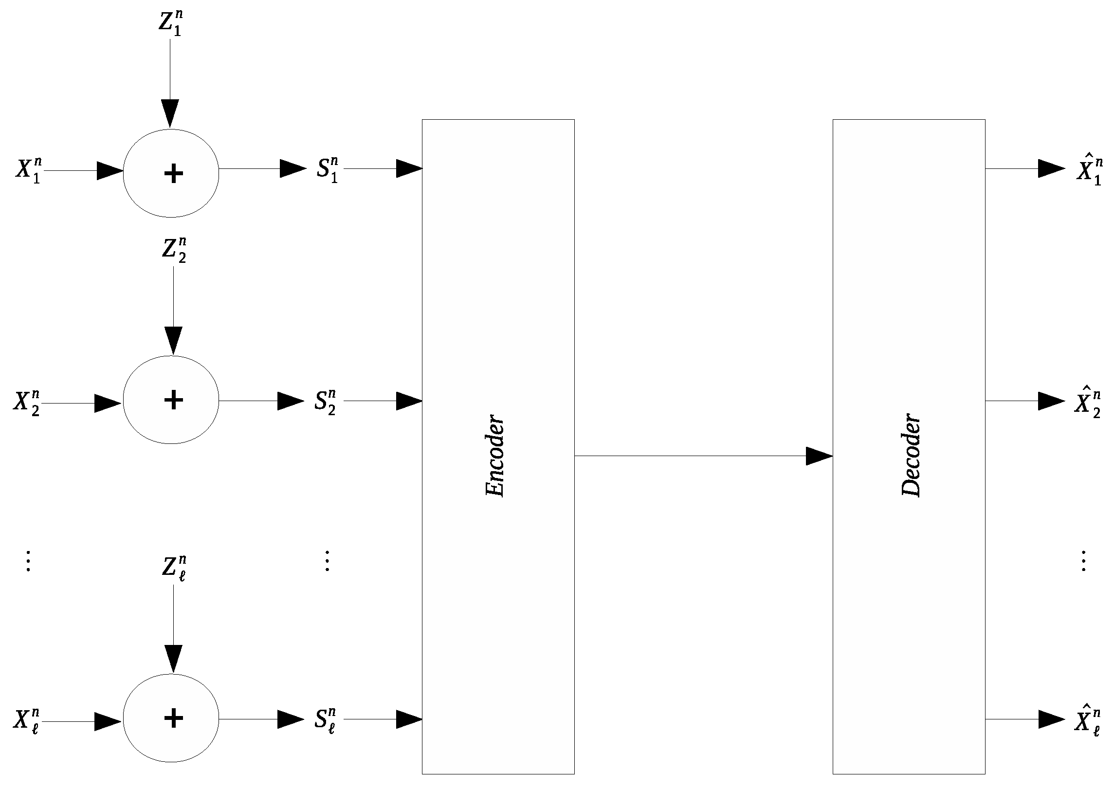
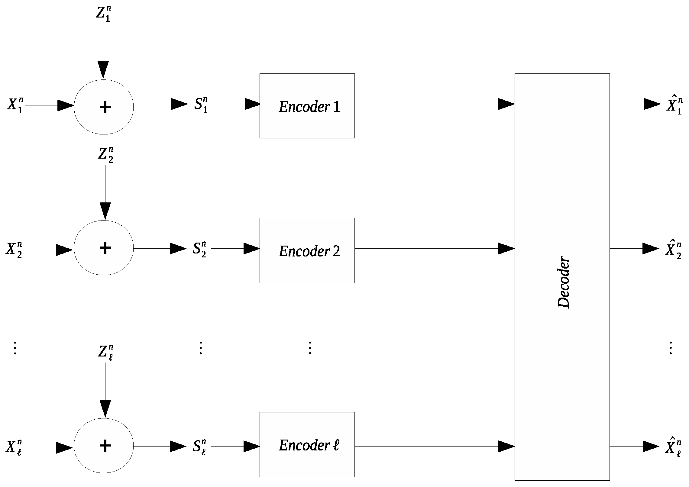
Many applications involve collection and transmission of potentially noise-corrupted data. It is often necessary to compress the collected data to reduce the transmission cost. The remote source coding problem aims to characterize the optimal scheme for such compression and the relevant information-theoretic limit. In this work we study a quadratic Gaussian version of the remote source coding problem, where compression is performed on the noise-corrupted components of a symmetric multivariate Gaussian source. A prescribed mean squared error distortion constraint is imposed on the reconstruction of the noise-free source components; moreover, it is assumed that the noises across different source components are independent and obey the same Gaussian distribution. Two scenarios are considered: centralized encoding (see Figure 1) and distributed encoding (see Figure 2). It is worth noting that the distributed encoding scenario is closely related to the CEO problem, which has been studied extensively [1,2,3,4,5,6,7,8,9,10,11,12,13,14,15,16,17,18].
The present paper is primarily devoted to the comparison of the rate-distortion functions associated with the aforementioned two scenarios. We are particularly interested in understanding how the rate penalty for distributed encoding (relative to centralized encoding) depends on the target distortion as well as the parameters of source and noise models. Although the information-theoretic results needed for this comparison are available in the literature or can be derived in a relatively straightforward manner, the relevant expressions are too unwieldy to analyze. For this reason, we focus on the asymptotic regime where the number of source components, denoted by ℓ, is sufficiently large. Indeed, it will be seen that the gap between the two rate-distortion functions admits a simple characterization in the large ℓ limit, yielding useful insights into the fundamental difference between centralized encoding and distributed coding, which are hard to obtain otherwise.
The rest of this paper is organized as follows. We state the problem definitions and the main results in Section 2. The proofs are provided in Section 3. We conclude the paper in Section 4.
Notation: The expectation operator and the transpose operator are denoted by and , respectively. An ℓ-dimensional all-one row vector is written as . We use as an abbreviation of . The cardinality of a set is denoted by . We write if the absolute value of is bounded for all sufficiently large ℓ. Throughout this paper, the base of the logarithm function is e, and .
2. Problem Definitions and Main Results
Let be the sum of two mutually independent ℓ-dimensional () zero-mean Gaussian random vectors, source and noise , with
where , , and . Moreover, let be i.i.d. copies of .
Definition 1 (Centralized encoding).
A rate-distortion pair is said to be achievable with centralized encoding if, for any , there exists an encoding function such that
where . For a given d, we denote by the minimum r such that is achievable with centralized encoding.
Definition 2 (Distributed encoding).
A rate-distortion pair is said to be achievable with distributed encoding if, for any , there exist encoding functions , , such that
where . For a given d, we denote by the minimum r such that is achievable with distributed encoding.
We will refer to as the rate-distortion function of symmetric remote Gaussian source coding with centralized encoding, and as the rate-distortion function of symmetric remote Gaussian source coding with distributed encoding. It is clear that for any d since distributed encoding can be simulated by centralized encoding. Moreover, it is easy to show that for (since the distortion constraint is trivially satisfied with the reconstruction set to be zero) and for (since is the minimum achievable distortion when is directly available at the decoder), where (see Section 3.1 for a detailed derivation)
with . Henceforth we shall focus on the case .
Lemma 1.
For ,
where
Proof.
See Section 3.1. □
Lemma 2.
For ,
where
with
The expressions of and as shown in Lemmas 1 and 2 are quite complicated, rendering it difficult to make analytical comparisons. Fortunately, they become significantly simplified in the asymptotic regime where (with d fixed). To perform this asymptotic analysis, it is necessary to restrict attention to the case ; moreover, without loss of generality, we assume , where
Theorem 1 (Centralized encoding).
- 1.
- : For ,
- 2.
- : For ,where
Proof.
See Section 3.2. □
Theorem 2 (Distributed encoding).
- 1.
- : For ,
- 2.
- : For ,where
Proof.
See Section 3.3. □
Remark 1.
The following result is a simple corollary of Theorems 1 and 2.
Corollary 1 (Asymptotic gap).
- 1.
- : For ,
- 2.
- : For ,
Remark 2.
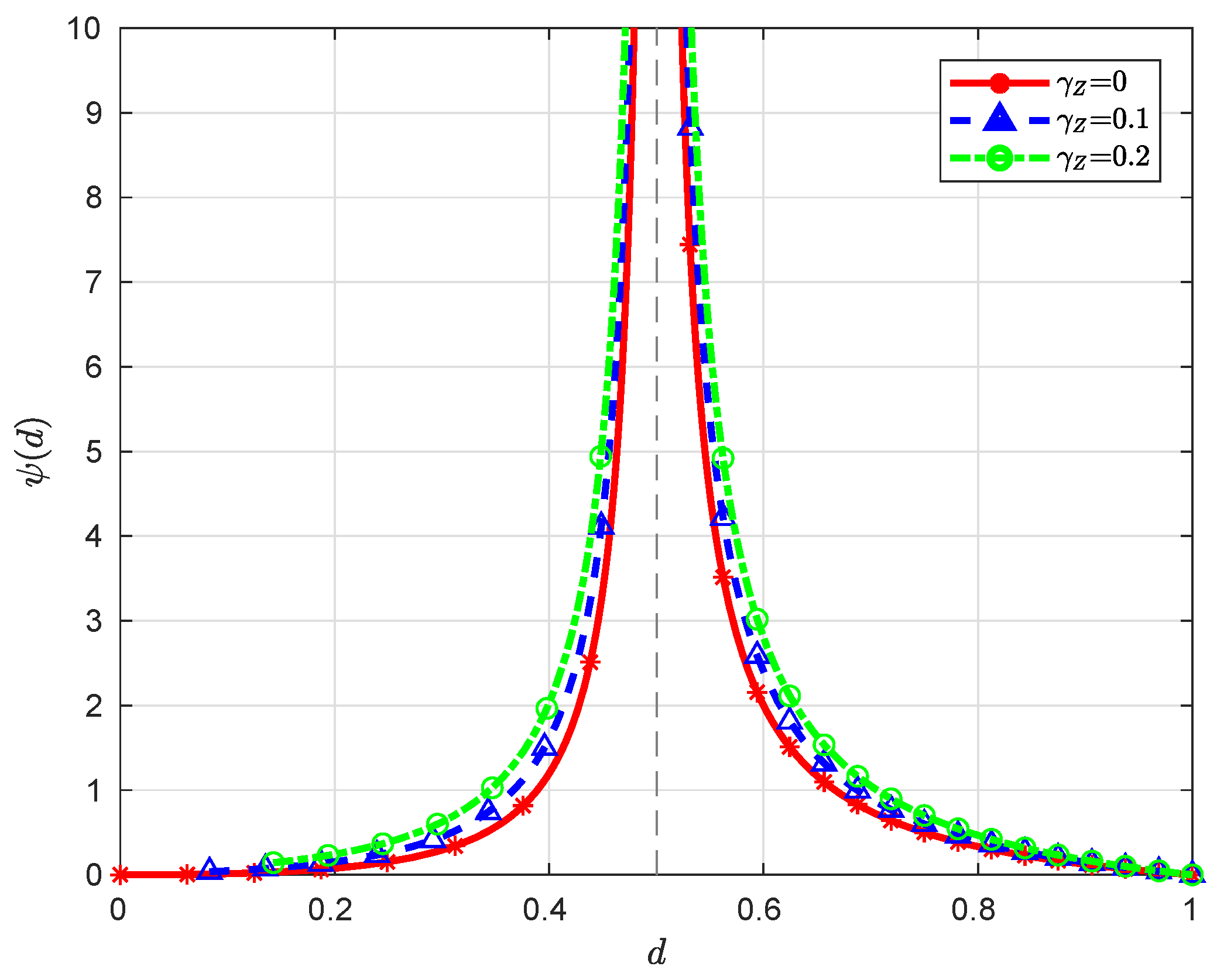
When , we have , which is a monotonically decreasing function over , converging to ∞ (here we assume ) and 0 as and , respectively. When , it is clear that the function is monotonically decreasing over , converging to ∞ and 0 as and , respectively; moreover, since for , the function is monotonically increasing over , converging to and ∞ as and , respectively. Note that for ; therefore, the minimum value of over is 0, which is attained at . See Figure 3 and Figure 4 for some graphical illustrations of .
3. Proofs
3.1. Proof of Lemma 1
It is known [21] that is given by the solution to the following optimization problem:
Let , , and , where is an arbitrary (real) unitary matrix with the first row being . Since unitary transformations are invertible and preserve the Euclidean norm, we can write equivalently as
For the same reason, we have
Denote the i-th components of , , and by , , and , respectively, . Clearly, , . Moreover, it can be verified that are independent zero-mean Gaussian random variables with
Now denote the i-th component of by , . We have
and
Clearly, is determined by ; moreover, for any ℓ-dimensional random vector jointly distributed with such that form a Markov chain, we have
Therefore, is equivalent to
One can readily complete the proof of Lemma 1 by recognizing that the solution to is given by the well-known reverse water-filling formula ([22] Theorem 13.3.3).
3.2. Proof of Theorem 1
Setting in Lemma 1 gives
for . Setting in Lemma 1 gives
for ; moreover, we have
and as .
It remains to treat the case . In this case, it can be deduced from Lemma 1 that
and we have
Consider the following two subcases separately.
3.3. Proof of Theorem 2
One can readily prove part one of Theorem 2 by setting in Lemma 2. So only part two of Theorem 2 remains to be proved. Note that
where
We shall consider the following three cases separately.
- In this case and consequentlywhen ℓ is sufficiently large. Note thatSubstituting (15) into (14) givesIt is easy to show thatCombining (16), (17) and (18) yieldswhereMoreover, it can be verified via algebraic manipulations thatNow we write equivalently asNote thatandSubstituting (20) and (21) into (19) gives
- In this case and consequentlywhen ℓ is sufficiently large. Note thatSubstituting (27) into (26) givesIt is easy to show thatCombining (28) and (29) yieldsNow we proceed to derive an asymptotic expression of . Note thatandSubstituting (30) and (31) into (19) givesThis completes the proof of Theorem 2.
4. Conclusions
We have studied the problem of symmetric remote Gaussian source coding and made a systematic comparison of centralized encoding and distributed encoding in terms of the asymptotic rate-distortion performance. It is of great interest to extend our work by considering more general source and noise models.
Author Contributions
Conceptualization, Y.W. and J.C.; methodology, Y.W.; validation, L.X., S.Z. and M.W.; formal analysis, L.X., S.Z. and M.W.; investigation, L.X., S.Z. and M.W.; writing—original draft preparation, Y.W.; writing—review and editing, J.C.; supervision, J.C.
Funding
S.Z. was supported in part by the China Scholarship Council.
Acknowledgments
The authors wish to thank the anonymous reviewer for their valuable comments and suggestions.
Conflicts of Interest
The authors declare no conflict of interest.
References
- Berger, T.; Zhang, Z.; Viswanathan, H. The CEO problem. IEEE Trans. Inf. Theory 1996, 42, 887–902. [Google Scholar] [CrossRef]
- Viswanathan, H.; Berger, T. The quadratic Gaussian CEO problem. IEEE Trans. Inf. Theory 1997, 43, 1549–1559. [Google Scholar] [CrossRef]
- Oohama, Y. The rate-distortion function for the quadratic Gaussian CEO problem. IEEE Trans. Inf. Theory 1998, 44, 1057–1070. [Google Scholar] [CrossRef]
- Prabhakaran, V.; Tse, D.; Ramchandran, K. Rate region of the quadratic Gaussian CEO problem. In Proceedings of the IEEE International Symposium onInformation Theory, Chicago, IL, USA, 27 June–2 July 2004; p. 117. [Google Scholar]
- Chen, J.; Zhang, X.; Berger, T.; Wicker, S.B. An upper bound on the sum-rate distortion function and its corresponding rate allocation schemes for the CEO problem. IEEE J. Sel. Areas Commun. 2004, 22, 977–987. [Google Scholar] [CrossRef] [Green Version]
- Oohama, Y. Rate-distortion theory for Gaussian multiterminal source coding systems with several side informations at the decoder. IEEE Trans. Inf. Theory 2005, 51, 2577–2593. [Google Scholar] [CrossRef]
- Chen, J.; Berger, T. Successive Wyner-Ziv coding scheme and its application to the quadratic Gaussian CEO problem. IEEE Trans. Inf. Theory 2008, 54, 1586–1603. [Google Scholar] [CrossRef]
- Wagner, A.B.; Tavildar, S.; Viswanath, P. Rate region of the quadratic Gaussian two-encoder source-coding problem. IEEE Trans. Inf. Theory 2008, 54, 1938–1961. [Google Scholar] [CrossRef]
- Tavildar, S.; Viswanath, P.; Wagner, A.B. The Gaussian many-help-one distributed source coding problem. IEEE Trans. Inf. Theory 2010, 56, 564–581. [Google Scholar] [CrossRef]
- Wang, J.; Chen, J.; Wu, X. On the sum rate of Gaussian multiterminal source coding: New proofs and results. IEEE Trans. Inf. Theory 2010, 56, 3946–3960. [Google Scholar] [CrossRef]
- Yang, Y.; Xiong, Z. On the generalized Gaussian CEO problem. IEEE Trans. Inf. Theory 2012, 58, 3350–3372. [Google Scholar] [CrossRef]
- Wang, J.; Chen, J. Vector Gaussian two-terminal source coding. IEEE Trans. Inf. Theory 2013, 59, 3693–3708. [Google Scholar] [CrossRef]
- Courtade, T.A.; Weissman, T. Multiterminal source coding under logarithmic loss. IEEE Trans. Inf. Theory 2014, 60, 740–761. [Google Scholar] [CrossRef]
- Wang, J.; Chen, J. Vector Gaussian multiterminal source coding. IEEE Trans. Inf. Theory 2014, 60, 5533–5552. [Google Scholar] [CrossRef]
- Oohama, Y. Indirect and direct Gaussian distributed source coding problems. IEEE Trans. Inf. Theory 2014, 60, 7506–7539. [Google Scholar] [CrossRef]
- Nangir, M.; Asvadi, R.; Ahmadian-Attari, M.; Chen, J. Analysis and code design for the binary CEO problem under logarithmic loss. IEEE Trans. Commun. 2018, 66, 6003–6014. [Google Scholar] [CrossRef]
- Ugur, Y.; Aguerri, I.-E.; Zaidi, A. Vector Gaussian CEO problem under logarithmic loss and applications. arXiv, 2018; arXiv:1811.03933. [Google Scholar]
- Nangir, M.; Asvadi, R.; Chen, J.; Ahmadian-Attari, M.; Matsumoto, T. Successive Wyner-Ziv coding for the binary CEO problem under logarithmic loss. arXiv, 2018; arXiv:1812.11584. [Google Scholar]
- Wang, Y.; Xie, L.; Zhang, X.; Chen, J. Robust distributed compression of symmetrically correlated Gaussian sources. arXiv, 2018; arXiv:1807.06799. [Google Scholar]
- Chen, J.; Xie, L.; Chang, Y.; Wang, J.; Wang, Y. Generalized Gaussian multiterminal source coding: The symmetric case. arXiv, 2017; arXiv:1710.04750. [Google Scholar]
- Dobrushin, R.; Tsybakov, B. Information transmission with additional noise. IRE Trans. Inf. Theory 1962, 8, 293–304. [Google Scholar] [CrossRef]
- Cover, T.; Thomas, J.A. Elements of Information Theory; Wiley: New York, NY, USA, 1991. [Google Scholar]
Figure 1.
Symmetric remote Gaussian source coding with centralized encoding.

Figure 2.
Symmetric remote Gaussian source coding with distributed encoding.

Figure 3.
Illustration of with and for different .

Figure 4.
Illustration of with and for different .

© 2019 by the authors. Licensee MDPI, Basel, Switzerland. This article is an open access article distributed under the terms and conditions of the Creative Commons Attribution (CC BY) license (http://creativecommons.org/licenses/by/4.0/).
Share and Cite
MDPI and ACS Style
Wang, Y.; Xie, L.; Zhou, S.; Wang, M.; Chen, J. Asymptotic Rate-Distortion Analysis of Symmetric Remote Gaussian Source Coding: Centralized Encoding vs. Distributed Encoding. Entropy 2019, 21, 213. https://doi.org/10.3390/e21020213
AMA Style
Wang Y, Xie L, Zhou S, Wang M, Chen J. Asymptotic Rate-Distortion Analysis of Symmetric Remote Gaussian Source Coding: Centralized Encoding vs. Distributed Encoding. Entropy. 2019; 21(2):213. https://doi.org/10.3390/e21020213
Chicago/Turabian StyleWang, Yizhong, Li Xie, Siyao Zhou, Mengzhen Wang, and Jun Chen. 2019. "Asymptotic Rate-Distortion Analysis of Symmetric Remote Gaussian Source Coding: Centralized Encoding vs. Distributed Encoding" Entropy 21, no. 2: 213. https://doi.org/10.3390/e21020213
Note that from the first issue of 2016, this journal uses article numbers instead of page numbers. See further details here.