Optimal Multiuser Diversity in Multi-Cell MIMO Uplink Networks: User Scaling Law and Beamforming Design


1
Department of Electronics Engineering, Chungnam National University, Daejeon 34134, Korea
2
Department of Electronics Engineering, Korea Polytechnic University, Siheung 15073, Korea
3
Department of Computer Science and Engineering, Dankook University, Yongin 448-701, Korea
4
School of Electrical and Computer Engineering, Ulsan National Institute of Science and Technology (UNIST)
*
Author to whom correspondence should be addressed.
Entropy 2017, 19(8), 393; https://doi.org/10.3390/e19080393
Submission received: 31 May 2017
/
Revised: 18 July 2017
/
Accepted: 27 July 2017
/
Published: 29 July 2017
(This article belongs to the Special Issue Network Information Theory)
Abstract
:We introduce a distributed protocol to achieve multiuser diversity in a multicell multiple-input multiple-output (MIMO) uplink network, referred to as a MIMO interfering multiple-access channel (IMAC). Assuming both no information exchange among base stations (BS) and local channel state information at the transmitters for the MIMO IMAC, we propose a joint beamforming and user scheduling protocol, and then show that the proposed protocol can achieve the optimal multiuser diversity gain, i.e., , as long as the number of mobile stations (MSs) in a cell, N, scales faster than for a small constant , where M, L, K, and denote the number of receive antennas at each BS, the number of transmit antennas at each MS, the number of cells, and the signal-to-noise ratio, respectively. Our result indicates that multiuser diversity can be achieved in the presence of intra-cell and inter-cell interference even in a distributed fashion. As a result, vital information on how to design distributed algorithms in interference-limited cellular environments is provided.
1. Introduction
1.1. Previous Work
Multiuser diversity has been studied by showing an asymptotic system throughput in terms of a large number of users via opportunistic scheduling in slow fading environments. Opportunistic scheduling was originally proposed in a single-cell uplink network [1], where a base station (BS) selects a single mobile station (MS) among multiple MSs whose channel gain is the largest. Furthermore, in [1], the optimal power control method was also proposed in order to maximize the average sum-rate capacity in the network model. In [2], opportunistic scheduling with beamforming was introduced in a single-cell downlink network, where multiple antennas are equipped at a BS and a single antenna is used at each MS. It was proved that the system throughput scales as when the number of MSs in a cell, N, increases. This asymptotic result is based on the extreme value theory in order statistics in the limit of large N [3]. In [4], a random beamforming technique adopting multiple beams was proposed for single-cell downlink, where the system throughput is shown to scale as , where M denotes the number of antennas at each BS. This throughput scaling is asymptotically optimal for the single-cell downlink setup since it contains both the multiuser diversity gain as well as the degrees of freedom gain [5].
On the one hand, interference management has been thought of as one of the most challenging issues in wireless networks. To solve interference problems, opportunistic scheduling techniques have been introduced for a variety of network scenarios in which inter-cell interference exists. For example, in multi-cell downlink networks, also known as interfering broadcast channels (IBCs), a multi-cell random beamforming technique was proposed in [6], where it was shown that the optimal multiuser diversity gain, i.e., , can be achieved even in the presence of inter-cell interference. Recently, it was shown that the same multiuser diversity gain as in [6] can be achieved by introducing an opportunistic downlink interference alignment [7], while much less MSs are required to guarantee the optimal multiuser diversity. In [7], a two-stage transmit beamforming technique at BSs and the receive beamforming technique at MSs in terms of minimizing the received interference from other cell BSs were presented. In particular, a semi-orthogonal user selection scheme was used for achieving the optimal multi-user diversity gain. Moreover, scenarios obtaining the multiuser diversity gain have been studied in ad hoc networks [8] and cognitive radio networks [9].
On the other hand, for multi-cell uplink networks, also known as interfering multiple-access channels (IMACs), which are subject to the dual of multi-cell downlink networks, finding a distributed way to achieve the optimal multiuser diversity is more challenging than the downlink case. This is because network coordination is difficult in practical systems assuming not only no information exchange among BSs but also local channel state information (CSI) at the transmitters. In [10], a distributed interference alignment (IA) technique was proposed for the K-user MIMO interference channel, where each transmitter adopts the beamforming vector such that the generating interference to other receivers is minimized except for its own receiver and each receiver adopts the beamforming vector such that the received interference from other transmitters is minimized except for its own transmitter. However, the distributed IA technique requires an iterative beamformer optimization for data transmission. The authors of [11] proved that the optimal multiuser diversity gain can be achieved by introducing a distributed user scheduling even in the presence of inter-cell interference when both MSs and BSs have a single antenna, which was later extended to the case deploying multiple antennas at each BS, i.e., the single-input multiple-output (SIMO) IMAC model [12]. When multiple antennas are deployed at both users and BSs, i.e., the multiple-input multiple-output (MIMO) IMAC model is assumed, however, how to achieve such diversity gain remains open to debate; it is a non-straightforward issue since one needs to jointly construct user scheduling as well as transmit/receive beamforming in a distributed manner while guaranteeing the optimal multiuser diversity gain. Recently, a joint beamforming and user scheduling framework was proposed in the MIMO IMAC model, where the transmit beamforming vector at users minimizes the generation of interference to other cell BSs and each BS selects the users with the minimum generating interference [13]. However, in [13], the optimal multi-user diversity gain was not analyzed whereas the user scaling law was analyzed for a given degree-of-freedom in the MIMO IMAC model.
1.2. Contributions
In this paper, we first propose a joint beamforming and user scheduling method (A part of this paper was presented at the IEEE PIMRC in 2014 [14].) as an achievable scheme in a time-division duplexing (TDD) K-cell MIMO IMAC model consisting of N MSs with L antennas and one BS with M antennas in a cell, which is well-suited to practical multi-cell MIMO uplink networks. Specifically, in the design of transmit/receive beamforming, each BS employs M random receive beamforming vectors, and each MS adopts a single singular value decomposition (SVD)-based beamforming vector that minimizes the sum of interference generation to its own cell and other cells. In each cell, based on two pre-determined thresholds (i.e., scheduling criteria), the BS selects M MSs such that both the sufficiently large desired signal power and sufficiently small generating interference power are guaranteed. Then, we show that the proposed method indeed achieves the optimal multiuser diversity gain provided that the two thresholds are properly determined and the number of per-cell MSs, N, is greater than a certain level for a small constant , where denotes the signal-to-noise ratio (SNR). Note that the the multiuser diversity can be achieved in the presence of intra-cell and inter-cell interference in a distributed manner, operating based on local CSI at each MS as in [10]. Simulation results show that the proposed method outperforms two distributed baseline schemes in terms of sum-rates under practical network environments.
1.3. Organization
The rest of the paper is organized as follows. Section 2 describes the system and channel models. The proposed joint beamforming and scheduling method is described in Section 3. In Section 4, the multiuser diversity gain achieved by the proposed method is analyzed. Numerical results are shown in Section 5. Finally, conclusions are drawn in Section 6.
1.4. Notation
Throughout this paper, and indicate the field of complex numbers and the statistical expectation, respectively. Matrices and vectors are indicated with boldface uppercase and lowercase letters, respectively. and denote the Hermitian transpose and the Frobenius norm, respectively, of the matrix . indicates the probability of the given event and denotes the identity matrix. Unless otherwise stated, all logarithms are assumed to be to the base 2. We use the following asymptotic notation: (i) means that there exist constants C and c such that for all ; (ii) means that ; (iii) if ; (iv) if and , (v) f(x)=(g(x)) if [15]. Some notations will be more precisely defined in the following sections.
2. System Model
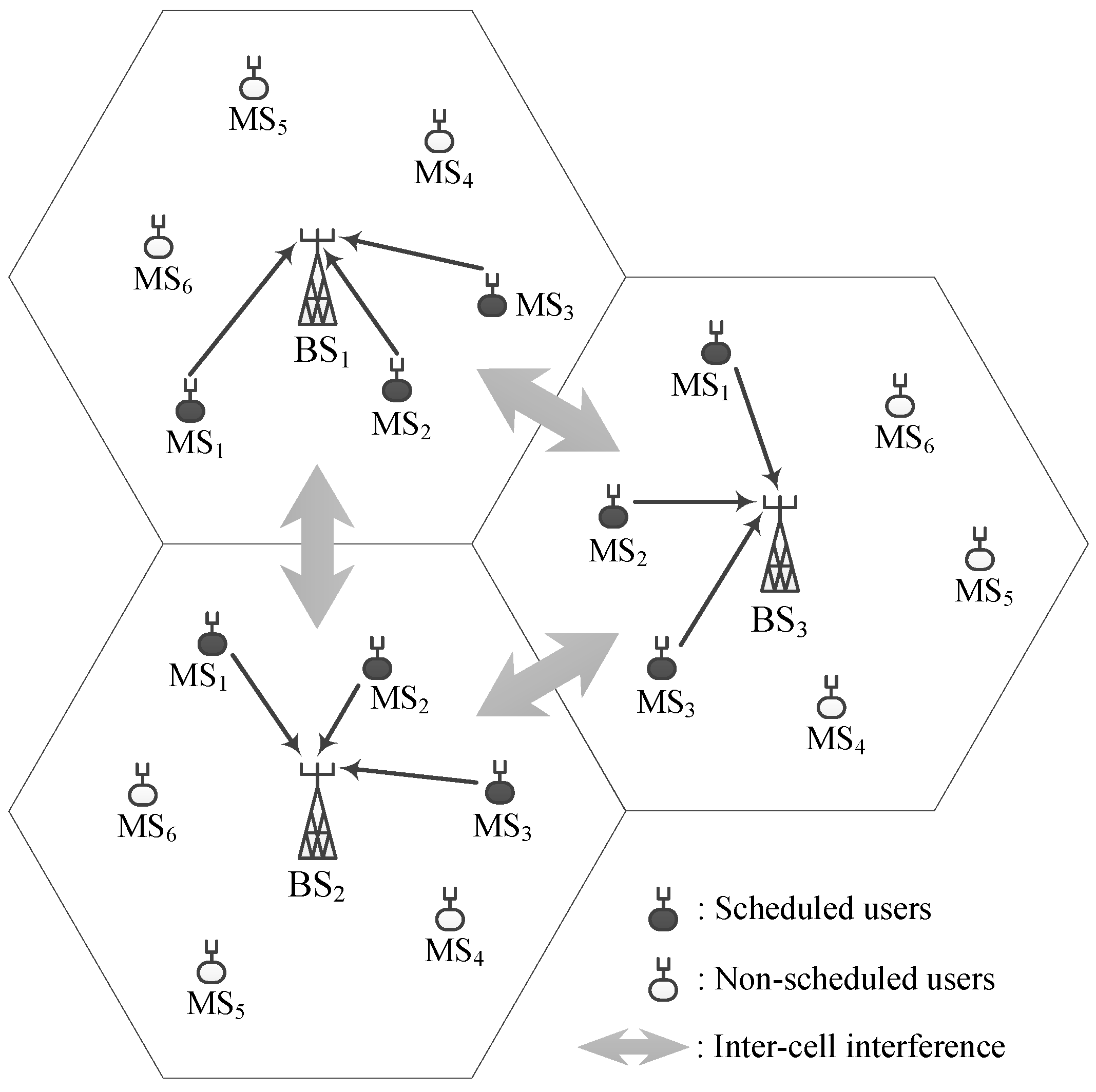
As illustrated in Figure 1, we consider a TDD K-cell MIMO IMAC model, where each cell consists of a single BS with M antennas and N users with L antennas each. We assume the block fading channel, where each channel coefficient remains unchanged during a transmission block (e.g., frame) and independently changes for every transmission block. Then, the received signal vector at the ith BS is given by
where denotes the large-scale path-loss gain from the jth MS in the ith cell to the kth BS (in the kth cell). Here, , where represents the distance between the jth MS in the ith cell to the kth BS and denotes the path-loss exponent. In addition, denotes the small-scale fading channel matrix from the jth MS in the ith cell to the kth BS, each element of which is assumed to be an independent and identically distributed (i.i.d.) standard complex Gaussian random variable. The transmit beamforming vector of the jth MS in the ith cell is denoted by , and denotes the transmitted symbol of the jth MS in the ith cell. We assume that each BS selects M MSs at each time slot and each selected MS sends a spatial stream with . The additive white Gaussian noise (AWGN) at the ith BS is denoted by with zero mean and covariance matrix , i.e., . We denote .
3. A Joint Design of Beamforming and Scheduling
In this section, we describe our distributed beamforming and scheduling method for the MIMO IMAC model. The proposed method is constructed based on the two thresholds with regard to both desired signal and interference power levels. That is, we find the two threshold values such that the optimal multiuser diversity can be achieved (which will be shown in the next section).
Each BS first generates M random receive beamforming vectors orthogonal to each other, each of which is to serve each selected MS. A receiver beamfoming matrix for the ith BS, , is defined as
where denotes the mth orthonormal beamforming vector. These (pseudo-)randomly generated matrices are assumed to be known to all MSs in the network. After receive beamforming, the received signal vector at the ith BS, , is rewritten as
where denotes the index of a scheduled MS for the mth receive beamforming vector in the ith cell and . Then, the received signal for the th receive beamforming vector of the ith BS is expressed as
where .
From the channel reciprocity between downlink and uplink, it is possible for the jth MS in the ith cell to obtain all the received channel matrices , , by using downlink pilot signaling transmitted from the BSs. To be scheduled, the jth MS in the ith cell finds the index satisfying the following two criteria:
where and denote the pre-determined positive threshold values. The transmit beamforming vector is to be designed in the sequel to minimize the sum-interference. Criterion is satisfied if the desired signal power strength is greater than or equal to , which is set in such a way that the MSs’ desired signal power received at the corresponding BS is sufficiently large to obtain the multiuser diversity gain. On the other hand, criterion is satisfied if the sum of interference power levels generated by the MS to its own BS (i.e., the intra-cell interference) and other BSs (i.e., the inter-cell interference) is less than or equal to , which is set to a sufficiently small value to ensure that the cross-channels of the selected MS are in deep fade, while not preventing the system from obtaining multiuser diversity. The left-hand side of (3) accounts for the sum power of intra-cell and inter-cell interference power levels generated by the jth MS, termed leakage of interference (LIF). The LIF of the jth MS in the ith cell for the th receive beamforming vector is defined as
If an MS has at least one index , for which both the criteria and are satisfied, then it feeds back the corresponding indices and their scheduling metrics of (2) and (3) to the BS. Otherwise, it feeds back nothing. For each , each BS randomly selects one MS among the MSs that have fed back the same beamforming vector index . Finally, the selected MSs in each cell transmit their uplink data, and each BS then decodes the MSs’ signals while treating all the intra-cell and inter-cell interference as noise.
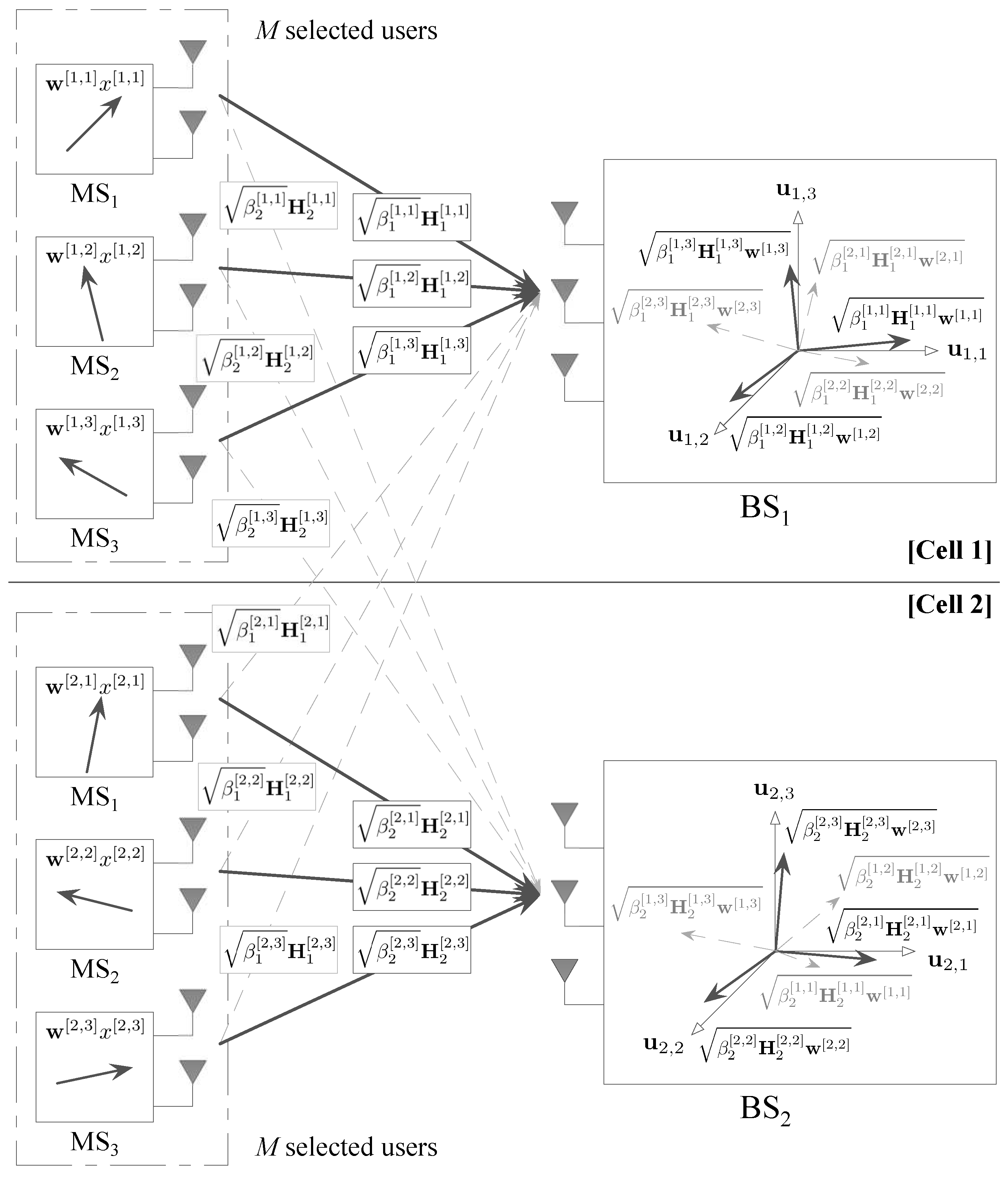
Figure 2 shows a geometric interpretation of the proposed scheme.
4. Analysis of Multiuser Diversity
In this section, we analyze the multiuser diversity gain achieved by the joint beamforming and scheduling method in Section 3, which enables us to obtain the asymptotic sum-rate scaling under the condition of the number of per-cell MSs, N. In the following theorem, we establish our main result.
Theorem 1.
Suppose that for a constant and . Then, for the K-cell MIMO IMAC model, the sum-rate achieved by the proposed method in Section 3 scales as with high probability in a high SNR regime if .
Proof.
Refer to Appendix for the proof. ☐
It is worth noting that the proof technique used to achieve the sum-rate scaling in this paper is fundamentally different from the SIMO IMAC case in [12] in the sense that the MS (transmitter) performs the SVD-based transmit beamforming to minimize the effective interference including both the inter-cell interference to other cells and the intro-cell interference to its own cell, whereas there is no such optimization process in the SIMO case. From our main result, the following two comparisons are made.
Remark 1.
[Comparison with the SISO and SIMO IMAC] If a single antenna is adopted at both MS and BS sides, i.e., the single-input single-output (SISO) IMAC model is assumed, then the required user scaling law for achieving the optimal multiuser diversity gain becomes by setting , which is consistent with the result in [11]. Furthermore, if a single antenna at the MS sides but multiple antennas at the BSs are adopted, i.e., the SIMO IMAC model is assumed, then the required user scaling law for achieving the optimal multiuser diversity gain becomes by setting , which is also consistent with the result in [12].
Remark 2.
[Comparison with the antenna selection] If a transmit antenna selection strategy is used instead of the SVD-based transmit beamforming at the MSs, then the achievable sum-rate scales as with high probability in the high SNR regime under the condition of , which can be obtained from [12] by regarding each antenna at the MS as an independent user. Note that the antenna selection only reduces the required number of MSs by a factor of (which is a constant), compared to the SIMO IMAC case.
Remark 3.
[Application to massive MIMO systems] Consider the case that very large antenna arrays are equipped, i.e., , and the random beamforming is utilized at BSs. In addition, we assume that the number of scheduled users, denoted by S, is much smaller than the number of antennas at BSs, i.e., . Then, both inter-cell interference and intra-cell interference can be nulled out regardless of the transmit beamforming vector at MSs, as shown in [16]. Therefore, the optimal transmit beamforming at MSs is to maximize the received signal strength, while the transmit beamforming in the proposed technique is to minimize the generating interference. For a particular (random) beam at a BS, the optimal user scheduling algorithm is to select the user with the maximum signal strength in this case.
5. Numerical Evaluation
For performance comparison, five baseline schemes are shown: max-SNR, min-LIF, MIMO IMAC opportunistic IA (OIA) [13], max-signal-to-generating-interference-plus-noise (SGINR) [17], and SIMO case [12]. In the max-SNR scheme, the transmit beamforming vector is designed as to maximize the desired channel gain and the MSs with higher desired channel gains are selected. In the min-LIF scheme, the design of beamforming vector as well as the user scheduling is performed only to minimize the LIF in (4). In the MIMO IMAC OIA scheme, the min-LIF based beamforming is employed at each MS to suppress the intercell interference while a zero-forcing filtering is used at each BS to completely remove the intra-cell interference [13]. Note that the OIA scheme adopts the channel-adaptive ZF receiver at the BSs, while the proposed method in this paper adopts the random receive beamforming technique at the BSs. Thus, the proposed method has less computational complexity at the receiver end while having the same complexity at the MS, compared with the MIMO IMAC OIA scheme [13]. In the max-SGINR scheme [17], the beamforming vector and user selection are designed in the sense of maximizing the SGINR metric, which can be computed based only on local CSI. For fair comparison to the proposed scheme, where no vector feedback is required, antenna selection is used in simulations.
We modify the proposed method so that it is suitable for numerical evaluation. Specifically, criterion (C1) is replaced by choosing M MSs with up to the Mth highest value of among the MSs satisfying another criterion (C2). This modification can be regarded as a special case of the original proposed method in Section 3 by setting (rather than ) and choosing M MSs having the maximum desired channel gain. Thus, it is obvious that the original proposed method indeed achieves the same sum-rates as those of the modified one in finite SNR or N regimes.
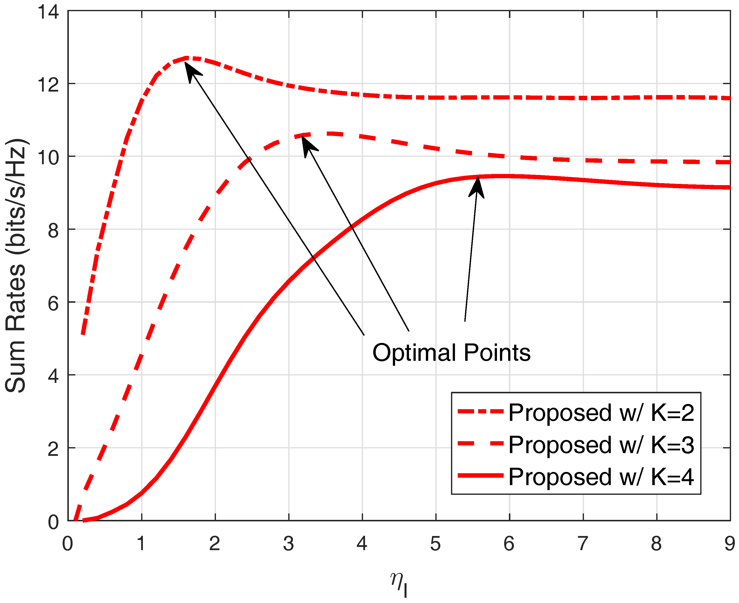
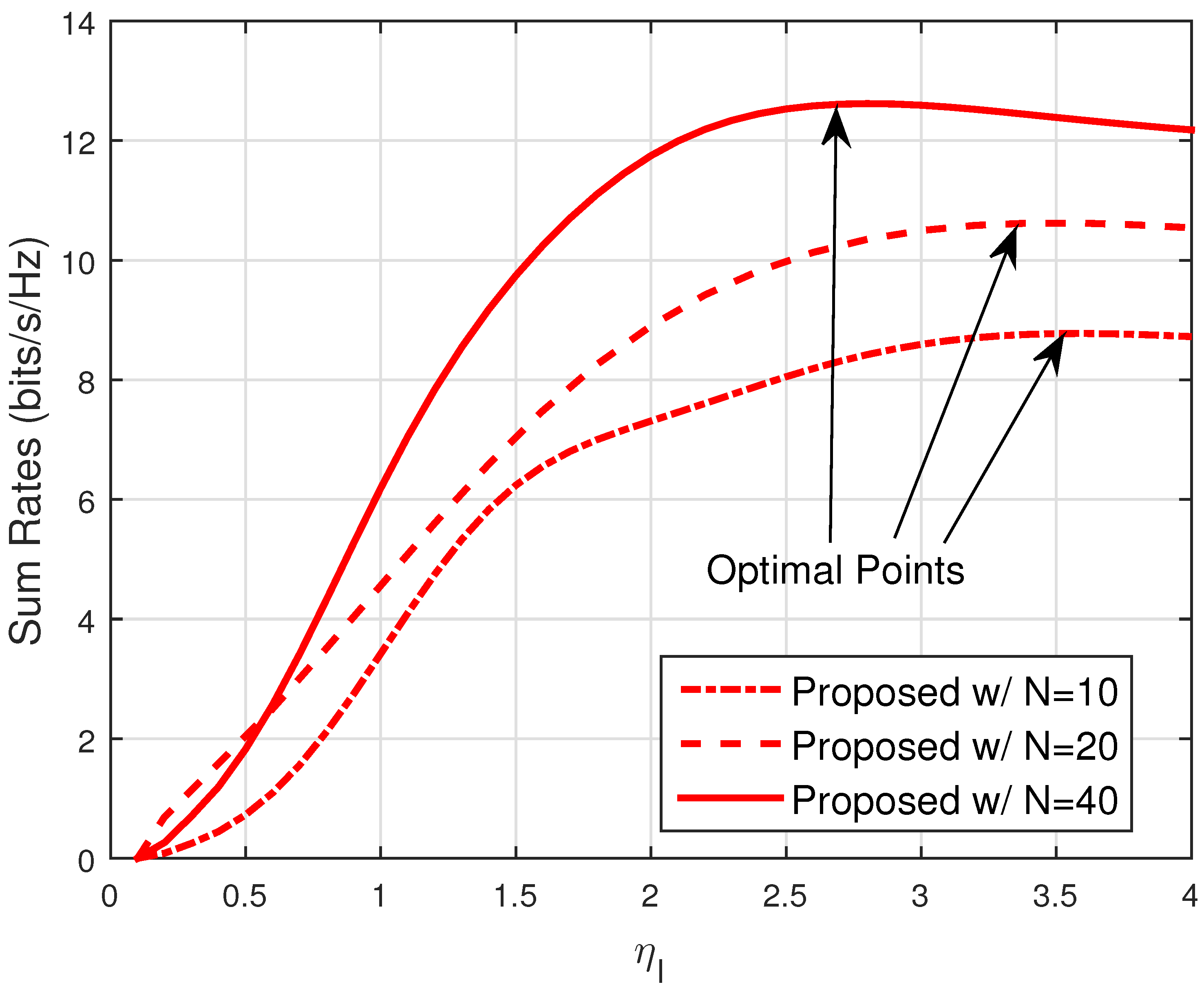
Figure 3 and Figure 4 show sum-rates versus for various K and N values, respectively, where and dB. In the proposed method, the optimal can be numerically found for given parameters. As shown in Figure 3, the optimal grows with increasing K due to the effect of stronger inter-cell interference. On the other hand, the optimal reduces with increasing N, as depicted in Figure 4, since the inter-cell interference can be more suppressed for larger N with the help of the multiuser diversity gain. For example, the optimal maximizing the sum rate is equal to , and when , 20 and 30, respectively. With the optimal , the maximum sum-rate is equal to , and , respectively.
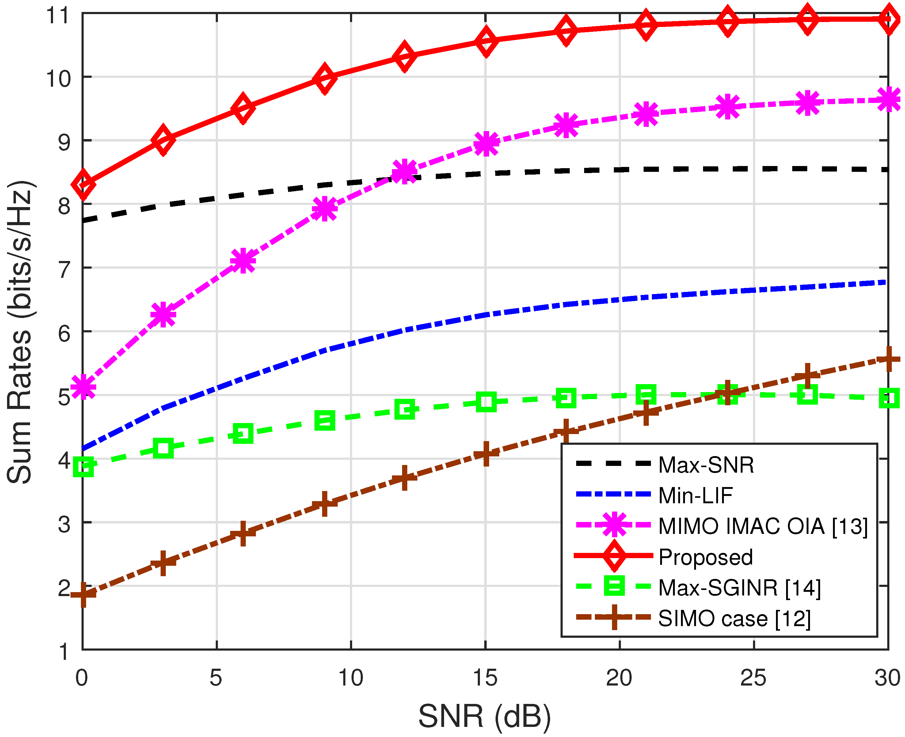
Figure 5 depicts sum-rates versus SNR for , , and . In the proposed method, is optimized for each N and SNR. The sum-rate of the max-SNR shows only a marginal improvement with respect to SNR due to the residual interference level. The proposed method effectively suppresses the interference level while obtaining the sufficiently high desired channel gains simultaneously. It is shown that the proposed method yields higher sum-rates for all SNR regimes than those of the baseline schemes, whereas the MIMO IMAC OIA scheme [13] is even inferior to the max-SNR scheme in a low SNR regime since it cannot obtain the power gain. In particular, it is shown that, in comparison to the SIMO case, the proposed transmit beamforming design improves the sum-rate significantly even with one additional scalar value feedback from each user.
6. Concluding Remarks
In this paper, we introduced a joint design of beamforming and scheduling in the MIMO IMAC, where there is no information exchange among BSs and only local CSI is available at the transmitters. We showed that the proposed method achieves the optimal multiuser diversigy gain provided that the number of per-cell MSs, N, scales faster than for a small constant . The numerical results revealed that in a practical setting of the MIMO IMAC model, the proposed method outperforms the three baseline schemes in terms of sum-rates.
Acknowledgments
This work was partly supported by Institute for Information & communications Technology Promotion(IITP) grant funded by the Korea government(MSIT) (No. B0126-17-1064, Research on Near-Zero Latency Network for 5G Immersive Service), IITP grant funded by the Korea government (MSIT) (No. 2014-0-00282, Development of 5G Mobile Communication Technologies for Hyper-connected smart services), and the Basic Science Research Program through the National Research Foundation of Korea (NRF) funded by the Ministry of Science, ICT & Future Planning (MSIP) (2015R1A2A1A15054248).
Author Contributions
Bang Chul Jung conceived and designed the overall protocol, and analyzed the results; Su Min Kim wrote the paper and derived the main theorem; Won-Yong Shin designed the system model; Hyun Jong Yang wrote the simulation code and performed experiments.
Conflicts of Interest
The authors declare no conflict of interest.
Appendix A. Proof of Theorem 1
Proof:
The sum-rate is expressed as
where denotes the signal-to-interference-and-noise-ratio (SINR) for the MS selected for the th receive beamforming vector in the ith cell, i.e., th user in the ith cell. The sum-rate is then bounded by
where denotes the probability that at least one MS satisfying both the criteria and exists for the th receive beamforming vector at the ith BS.
From (2), the SINR of the th MS is given by
where
which represents the sum of intra-cell and inter-cell interference powers received at the th MS.
Now for given receive beamforming, each MS finds the optimal weight vector that minimizes its LIF metric in (4) by using the SVD-based beamforming. From (4), the LIF metric of the jth MS in the ith cell for a given receive beamforming vector is expressed as
where is given by
Here, is defined as
Let us denote the SVD of by
where and consist of L orthonormal columns, and for . Then, the optimal weight vector of the jth MS for the th beamforming vector is determined by
where denotes the Lth column of . Based on this weight vector design, an upper bound on the LIF metric in (A3) can be simplified to
From a similar argument to that in [13] (Lemma 1), it is not difficult to show that for , the CDF of , denoted by , can be written as
where is a constant determined by K, M and L.
Amongst N MSs in each cell, the probability that at least one MS satisfying both the criteria and exists is expressed as
Since the beamforming vector is an isotropically distributed unit-norm vector, each element of is an i.i.d. complex Gaussian random variable. In addition, is also a unit-norm vector, and hence is an i.i.d. complex Gaussian random variable. Thus, is exponentially distributed, and the probability that the th MS satisfies for the th beamforming vector is given by
Next, the probability that the th MS satisfies for the th beamforming vector is given by
where the inequality follows from for all and .
References
- Knopp, R.; Humblet, P. Information capacity and power control in single cell multiuser communications. In Proceedings of the IEEE International Conference on Communications (ICC), Seattle, WA, USA, 18–22 June 1995; pp. 331–335. [Google Scholar]
- Viswanath, P.; Tse, D.N.C.; Laroia, R. Opportunistic beamforming using dumb antennas. IEEE Trans. Inf. Theory 2002, 48, 1277–1294. [Google Scholar] [CrossRef]
- David, H.; Nagaraja, H. Order Statistics; Wiley: Hoboken, NJ, USA, 2003. [Google Scholar]
- Sharif, M.; Hassibi, B. On the capacity of MIMO broadcast channels with partial side information. IEEE Trans. Inf. Theory 2005, 51, 506–522. [Google Scholar] [CrossRef]
- Zheng, L.; Tse, D.N.C. Diversity and multiplexing: A fundamental tradeoff in multiple-antenna channels. IEEE Trans. Inf. Theory 2003, 49, 1073–1096. [Google Scholar] [CrossRef]
- Nguyen, H.D.; Zhang, R.; Hui, H.T. Multi-cell random beamforming: Achievable rate and degrees of freedom region. IEEE Trans. Signal Process. 2013, 61, 3532–3544. [Google Scholar] [CrossRef]
- Yang, H.J.; Shin, W.-Y.; Jung, B.C.; Suh, C.; Paulraj, A. Opportunistic downlink interference alignment for multi-cell MIMO networks. IEEE Trans. Wirel. Commun. 2017, 16, 1533–1548. [Google Scholar] [CrossRef]
- Shin, W.-Y.; Chung, S.-Y.; Lee, Y.H. Parallel opportunistic routing in wireless networks. IEEE Trans. Inf. Theory 2013, 59, 6290–6300. [Google Scholar] [CrossRef]
- Ban, T.W.; Choi, W.; Jung, B.C.; Sung, D.K. Multi-user diversity in a spectrum sharing system. IEEE Trans. Wirel. Commun. 2009, 8, 102–106. [Google Scholar] [CrossRef]
- Gomadam, K.; Cadambe, V.R.; Jafar, S.A. A distributed numerical approach to interference alignment and applications to wireless interference networks. IEEE Trans. Inf. Theory 2011, 57, 3309–3322. [Google Scholar] [CrossRef]
- Shin, W.-Y.; Park, D.; Jung, B.C. Can one achieve multiuser diversity in uplink multi-cell networks? IEEE Trans. Commun. 2012, 60, 3535–3540. [Google Scholar] [CrossRef]
- Shin, W.-Y.; Park, D.; Jung, B.C. On the multiuser diversity in SIMO interfering multiple access channels: Distributed user scheduling framework. J. Commun. Netw. 2015, 17, 267–274. [Google Scholar] [CrossRef]
- Yang, H.J.; Shin, W.-Y.; Jung, B.C.; Paulraj, A. Opportunistic interference alignment for MIMO interfering multiple-access channels. IEEE Trans. Wirel. Commun. 2013, 12, 2180–2192. [Google Scholar] [CrossRef]
- Jung, B.C.; Kim, S.M.; Yang, H.J.; Shin, W.-Y. On the joint design of beamforming and user scheduling in multi-cell MIMO uplink networks. In Proceedings of the IEEE Personal Indoor Mobile Radio Communication (PIMRC), Washington, DC, USA, 2–5 September 2014; pp. 502–506. [Google Scholar]
- Knuth, D.E. Big Omicron and big Omega and big Theta. ACM SIGACT News 1976, 8, 18–24. [Google Scholar] [CrossRef]
- Marzetta, T.L. Noncooperative cellular wireless with unlimited numbers of base station antennas. IEEE Trans. Wirel. Commun. 2010, 9, 3590–3600. [Google Scholar] [CrossRef]
- Lee, B.O.; Shin, O.-S.; Lee, K.B. Distributed user selection scheme for uplink multiuser MIMO systems in a multicell environment. EURASIP J. Wirel. Commun. Netw. 2012, 202, 1–10. [Google Scholar] [CrossRef]
Figure 1.
The multiple-input multiple-output (MIMO) interfering multiple-access channel (IMAC) model where , , , and .
Figure 1.
The multiple-input multiple-output (MIMO) interfering multiple-access channel (IMAC) model where , , , and .

Figure 2.
Geometrical illustration of the signal model. The geometric interpretation of the received signals at the BSs under the proposed method, where , , and (, , ).
Figure 2.
Geometrical illustration of the signal model. The geometric interpretation of the received signals at the BSs under the proposed method, where , , and (, , ).

Figure 3.
Simulation results on . Sum-rates versus for various K values with , , and dB.

Figure 4.
Simulation results on . Sum-rates versus for various N values with , , and dB.

Figure 5.
Simulation results on the sum-rates. Sum-rates versus SNR for , , and M = L = 3.

© 2017 by the authors. Licensee MDPI, Basel, Switzerland. This article is an open access article distributed under the terms and conditions of the Creative Commons Attribution (CC BY) license (http://creativecommons.org/licenses/by/4.0/).
Share and Cite
MDPI and ACS Style
Jung, B.C.; Kim, S.M.; Shin, W.-Y.; Yang, H.J. Optimal Multiuser Diversity in Multi-Cell MIMO Uplink Networks: User Scaling Law and Beamforming Design. Entropy 2017, 19, 393. https://doi.org/10.3390/e19080393
AMA Style
Jung BC, Kim SM, Shin W-Y, Yang HJ. Optimal Multiuser Diversity in Multi-Cell MIMO Uplink Networks: User Scaling Law and Beamforming Design. Entropy. 2017; 19(8):393. https://doi.org/10.3390/e19080393
Chicago/Turabian StyleJung, Bang Chul, Su Min Kim, Won-Yong Shin, and Hyun Jong Yang. 2017. "Optimal Multiuser Diversity in Multi-Cell MIMO Uplink Networks: User Scaling Law and Beamforming Design" Entropy 19, no. 8: 393. https://doi.org/10.3390/e19080393
Note that from the first issue of 2016, this journal uses article numbers instead of page numbers. See further details here.