Entropy Base Estimation of Moisture Content of the Top 10-m Unsaturated Soil for the Badain Jaran Desert in Northwestern China

Abstract

Estimation of soil moisture distribution in desert regions is challenged by the deep unsaturated zone and the extreme natural environment. In this study, an entropy-based method, consisting of information entropy, principle of maximum entropy (PME), solutions to PME with constraints, and the determination of parameters, is used to estimate the soil moisture distribution in the 10 m deep vadose zone of a desert region. Firstly, the soil moisture distribution is described as a scaled probability density function (PDF), which is solved by PME with the constraints of normalization, known arithmetic mean and geometric mean, and the solution is the general form of gamma distribution. A constant arithmetic mean is determined by considering the stable average recharge rate at thousand year scale, and an approximate constant geometric mean is determined by the low flow rate (about 1 cm a year). Followed, the parameters of the scaled PDF of gamma distribution are determined by local environmental factors like terrain and vegetation: the multivariate linear equations are established to qualify the relationship between the parameters and the environmental factors on the basis of nineteen random soil moisture profiles about depth through the application of fuzzy mathematics. Finally, the accuracy is tested using correlation coefficient (CC) and relative error. This method performs with CC larger than 0.9 in more than a half profiles and most larger than 0.8, the relative errors are less than 30% in most of soil moisture profiles and can be as low as less than 15% when parameters fitted appropriately. Therefore, this study provides an alternative method to estimate soil moisture distribution in top 0–10 m layers of the Badain Jaran Desert based on local terrain and vegetation factors instead of drilling sand samples, this method would be useful in desert regions with extreme natural conditions since these environmental factors can be obtained by remote sensing data. Meanwhile, we should bear in mind that this method is challenged in humid regions since more intensive and frequent precipitation, and more vegetation cover make the system much more complex.

1. Introduction

Soil moisture is a crucial factor in hydrologic, geomorphic, and pedogenic processes [1,2]. Moreover, it influences the partition of available energy between latent and sensible heat, and the magnitude of the net radiation absorption by the soil surface [3]. Under extremely dry conditions, both the number and the size of perennial plant species are limited by the availability of soil water [4,5]. Hence, it is necessary to know the soil moisture content in desert regions. A wide range of methods are used to measure the soil moisture, including mass soil water content by the drying method, volume moisture content by neutron probes, TDR probes, and remote sensing. However, these methods are challenged by the measurement of soil moisture in deep desert vadose zones. Soil moisture estimates are obtained within the top 5 cm depth by passive remote sensing [6] and at greater depths by active sensors, and a depth of tens of centimeters by TDR, whereas the depth of the vadose zone in desert regions is usually up to tens or hundreds of meters. The mass moisture content is limited by the huge amount of work as well as difficult natural conditions.

In recent years, entropy-based methods were used to estimate soil moisture in the vadose zone. Information content and complexity were used in soil water fluxes simulation [7]. Al-Hamdan and Cruise estimated the soil moisture profile to near 50 cm on the basis of PME [8]. Some infiltration equations were derived based on the principle of maximum entropy (PME) with the Shannon entropy or information entropy [9] as well as soil moisture movement on the basis of PME with Tsallis entropy [10]. The soil moisture distribution was also estimated in an irrigated field in North Central Alabama, USA, based on the PME [11]. These studies assumed that the vertical soil moisture distribution curve is a scaled probability density function (PDF) that follows PME. Then the PDF was solved using Lagrange multipliers with constraints of normalization and known mean.

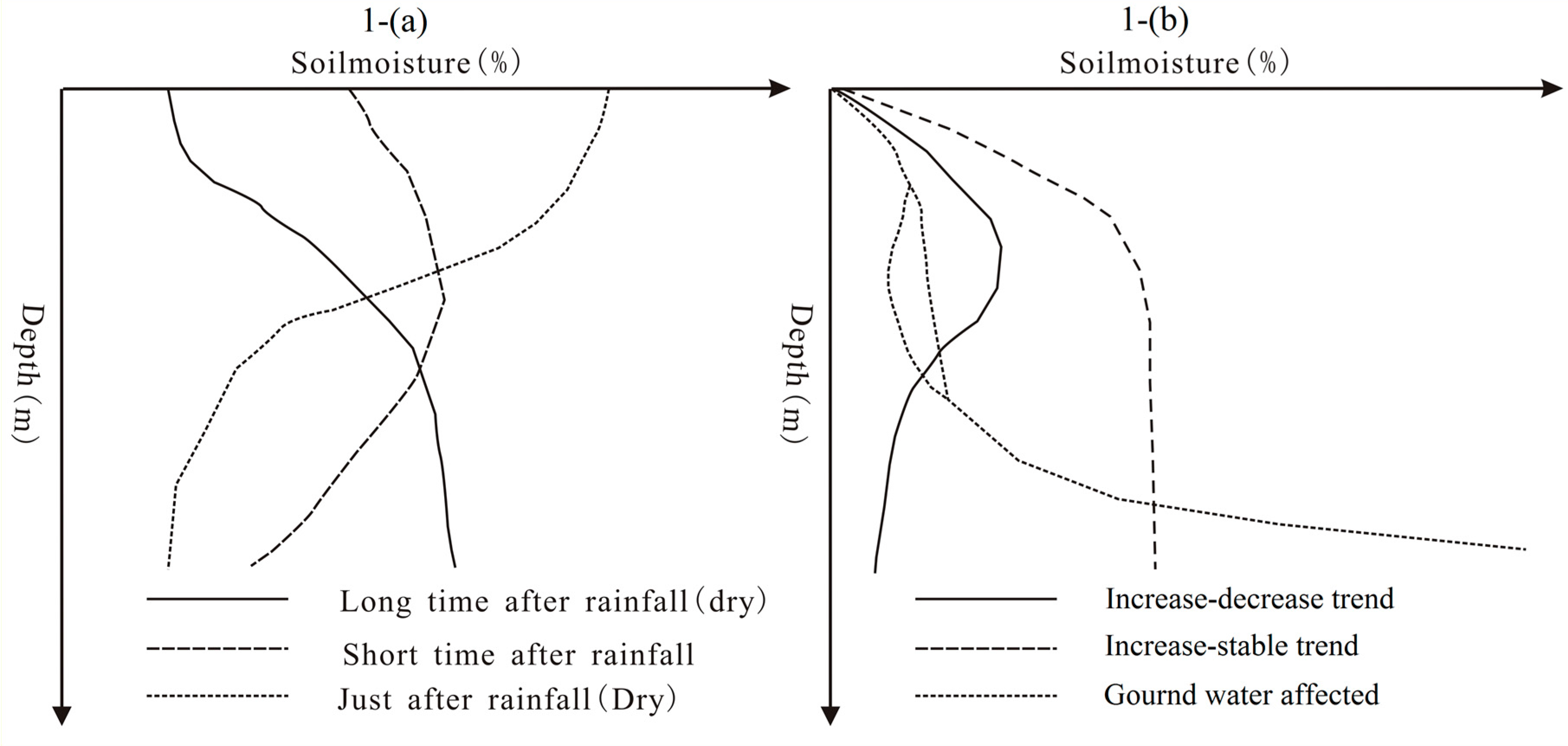
The soil water distribution in a vertical profile usually exhibits three phases, including just after rainfall (wet), a long time after rainfall (dry) and a short time after rainfall [9], which are illustrated in Figure 1a. However, some different characteristics were observed in the 10 m depth vadose zone of desert regions. Generally, the soil moisture profiles should be considered as the dry phase in desert areas as a result of the intense potential evaporation and little precipitation. Previous studies revealed that the distribution of soil moisture profiles have three subcategories in the deep vadose zone of the Badain Jaran Desert in Northeastern China, including an increase first then a decreasing trend, the increase then being stable and affected by ground water levels [12,13], as shown in Figure 1b.

The two former types are the typical moisture distribution in this region, corresponding to the distribution of a short time after rainfall and a long time after rainfall in the shallow soil layer, respectively. Therefore, these soil moisture distributions could be calculated by a method based on entropy theories. Singh considered the soil moisture distribution of a short time after rainfall (or lognormal distribution type) to consist of two parts: the dry case and the wet case [10]. This is only constrained by the limit of known information of the PDF (normalization and known mean) and the result is an exponential shaped curve. Further information is required to solve the soil moisture distribution curve similar to a two parameter probability distribution, such as gamma distribution, lognormal distribution and normal distribution. In desert regions, fortunately, the soil moisture distribution is a record of both precipitation and recharge history [14]. For example, a 10 m deep soil moisture profile is an archive of the climate change in the past 1000 years [15]. Hence, when sand texture and local environmental factors are determined, the total soil moisture in the deep vadose zone of the desert regions can be regarded as a constant since the difference between precipitation and evaporation is almost a constant on a thousand year scale. Apart from that, the geometric mean of the soil moisture curve is also a constant because the flow rate is extremely slow in desert regions. For example, the soil water recharge to ground water is about 1–1.3 mm per year in the Badian Jaran Desert [16]. Hence, the PDF-based distribution of soil moisture can be considered as a whole instead of two parts in this study area. Apart from that, soil moisture distribution is determined by the soil texture, local environmental factors like terrain and vegetation, and climatic factors [17]. In the deep desert vadose zone region, the texture is determined by the sand deposition and can be considered as constant at a small spatial scale; the vegetation is constricted by the soil moisture content in the top ten meters even as deep as dozens of meters, the climatic conditions are relatively uniform and is mostly affected by the terrain. Hence the system controlling soil moisture in desert regions is simpler than systems in humid regions, and establishing the relationship between soil moisture distribution and local surface controlling factors should be easier to achieve. A good correlation between the soil moisture distribution and local terrain and vegetation was revealed by geo-statistical analysis in the Badain Jara Desert [12,13].

Therefore, the objectives of this study are to: (1) consider the soil moisture distribution as an scaled entire probability distribution instead of two part in the deep vadose zone of the Badain Jaran Desert, and solve the distribution on the basis of PME with the constraints of normalization, known arithmetic mean and geometric mean; (2) determine the parameters of the scaled PDF based on local land surface factors like terrain and vegetation through the application of fuzzy mathematics methods, and to test the performance of this entropy-based method.

2. Study Area

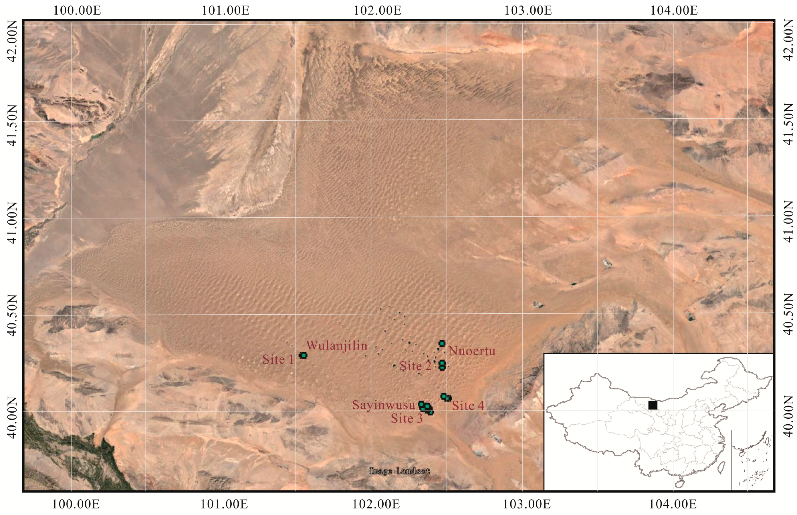
The Badain Jaran Desert is located in the northwestern part of the Alashan Plateau of western Inner Mongolia (39°20′N to 41°30′N and 100°E to 104°E; Figure 2), and covers an area of some 49,000 km² [18]. It contains the third largest dune field in China, and includes the highest megadunes on Earth. The dunes are interspersed with lakes that occur in many low-lying areas throughout the desert and that vary in size, shape, and salinity. From southeast to northwest the elevation gradually decreases from approximately 1800 m asl to 1000 m asl.

The climate in the Badain Jaran Desert is an extreme continental type, with hot summers and cold winters. Daily daytime temperatures in summer months range up to 40 °C, while mean monthly temperatures fall to −10 °C in January, and sub-zero minimum temperatures prevail for most of the year. The southeastern Badain Jaran Desert is near the current northern extent of the East Asian monsoon, which provides the primary source of precipitation, 70% of which falls from July to September. Rain falls on 10–35 days per year. Cold and dry continental air masses from the prevailing westerly winds dominate the region in the winter. The mean annual precipitation measured at the meteorological station nearest to the present study area (Zhongqanzi Station, 20 km southeast of the study area) was 84 mm from 1956 to 1999 and was highly variable (coefficient of variation = 0.39). In contrast, the potential evaporation from surface water is 2600 mm·year⁻¹ [19]. Average precipitation decreases significantly from south to north, declining to about 50 mm·year⁻¹ at Wentugaole, near the border between China and Mongolia [20], due to the progressively declining influence of monsoonal moisture. Orographic effects result in slightly higher rainfall rates in the Yabulai Mountains (150 mm·year⁻¹) in the southeastern part of the desert. The mean annual wind speed ranges from 2.8 to 4.6 m·s⁻¹, and increases from the south to the north, with the strongest winds in April and May.

3. Maximum Information Entropy Theories

3.1. Information Entropy

Information entropy or Shannon’s entropy of a random variable X with the PDF f(x) is defined as the negative expectation value of the logarithmic f(x) [21], usually denoted as H(x):

$$H(x)=-{\displaystyle \underset{a}{\overset{b}{\int }}f(x)\ln (f(x))dx}$$

(1)

$${\displaystyle \underset{a}{\overset{b}{\int }}f(x)dx=1}$$

(2)

where a is the minimum of variable X and b is the maximum of variable X.

The entropy of a single discrete random variable X is a measure of its average uncertainty, which is expressed by Equation (3):

$$H(x)=-{\displaystyle \sum _{i=1}^n{p}_i\ln (p_i})$$

(3)

where X represents a random variable with a set of values i and probability mass function p(x_i) = Pr(X = x_i). Note that p log p = 0 if p = 0.

3.2. Principle of Maximum Entropy and Probability Distribution

Principle of maximum entropy (PME) theory is used as a constructive criterion for setting up the least biased probability distribution based on partial knowledge [22,23]. If no other information is available except given statistical constraints, the distribution on the basis of PME is the least biased toward unavailable information. Therefore, the probability distributions are quite different with different constraints or known information. For the PDF f(x), the first constraint is the normalization, shown as Equation (2). Apart from that, the mean, variance or other information can be considered as known information for specific conditions. These constraints are denoted as g_i(x), which can be expressed as follows:

$${\displaystyle \underset{a}{\overset{b}{\int }}{g}_i(x)f(x)dx=G_i}$$

(4)

In order to solve f(x) with constrains of Equations (2) and (4), one simple method is using Lagrange multipliers to solve it under extreme conditions. The Lagrange function L can be defined as Equation (5):

$$L=-{\displaystyle \underset{a}{\overset{b}{\int }}f(x)\ln (f(x))dx}+{\lambda }_0({\displaystyle \underset{a}{\overset{b}{\int }}f(x)dx-1})+{\displaystyle \sum _{i=1}^n{\lambda }_i({\displaystyle \underset{a}{\overset{b}{\int }}{g}_i(x)f(x)dx-G_i}})$$

(5)

where λ₀, λ₁, λ₂, … ,λ_n are Lagrange multipliers. As the information entropy is the maximum value, the partial derivative function is equal to zero, as shown in Equations (6)–(8):

$$\frac{\partial L}{\partial f}=0$$

(6)

$$-\ln (f(x))-1+{\lambda }_0+{\displaystyle \sum _{i=1}^n{\lambda }_i{g}_i(x)}=0$$

(7)

$$f(x)=e^{-1+{\lambda }_0+{\displaystyle \sum _{i=1}^n{\lambda }_i{g}_i(x)}}$$

(8)

Equation (8) is the general PDF of random variable X solved by PME with the constraints of Equations (2) and (4). More details on the mathematical proof of the probability distribution based on PME can be found in Conrad [24].

4. Principle of Maximum Entropy for Soil Moisture Distribution in Deep Desert vadose Zone

The function between soil moisture and vertical soil depth can be written as:

$${\theta }_{\mathrm{Z}}=f(z)$$

(9)

where θ_Z is the soil moisture at depth z.

The accumulation of soil water:

$${\displaystyle {\int }_0^{Z}f(z)}dz=C$$

(10)

where C is the total soil water in a profile. Equation (10) can also be transformed as:

$${\displaystyle {\int }_0^Z\frac{1}{C}f(z)}dz=1$$

(11)

Hence the scaled vertical soil moisture distribution f(z)/C can be considered as a PDF. The information entropy can be calculated as:

$$H=-{\displaystyle {\int }_0^Z\frac{1}{C}f(z)\ln \frac{f(z)}{C}}dz$$

(12)

$$H=-\frac{1}{C}{\displaystyle {\int }_0^{Z}f(z)\ln f(z)}dz+\frac{1}{C}\ln C$$

(13)

As the soil water can be seen as in an equilibrium state, the function f(z)/C obeys the principle of maximum entropy, and the constraints of f(z)/C are: (1) the normalization; (2) arithmetic mean is given since the average recharge rate or the average recharge depth at millennium scale is a constant; (3) geometric mean can be considered as a constant since flow rate is get close to zero and the soil moisture also can be approximately considered as an equilibrium state in desert regions, which are shown in Equations (11), (14) and (15):

$${\displaystyle {\int }_0^Z\frac{z}{C}f(z)}dz={\mu }_z$$

(14)

$${\displaystyle {\int }_0^Z\frac{\ln (z)}{C}f(z)}dz={\nu }_z$$

(15)

where μ_z and ν_z and are the arithmetic mean and geometric mean of soil moisture distribution, respectively. Then we construct the Lagrange function L with the constraints of (11), (14) and (15):

$$\begin{array}{l}L=-\frac{1}{C}{\displaystyle {\int }_0^{Z}f(z)\ln f(z)}dz+\frac{1}{C}\ln C+{\lambda }_0({\displaystyle {\int }_0^Z\frac{1}{C}f(z)}dz-1)\\ +{\lambda }_1({\displaystyle {\int }_0^Z\frac{z}{C}f(z)}dz-{\mu }_z)+{\lambda }_2({\displaystyle {\int }_0^Z\frac{\ln (z)}{C}f(z)}dz-{\nu }_z)\end{array}$$

(16)

Let $\frac{\partial L}{\partial f_z}=0$, we can find the probability density function f(z)/C:

$$f(z)/C=e^{{\lambda }_0-1+{\lambda }_{1}z+{\lambda }_2\ln z}$$

(17)

Substituting Equation (17) into Equations (11), (14) and (15), we can obtain the values of λ₀, λ₁, λ₂. Equation (17) can also be transformed as (18):

$$f(z)/C=e^{{\lambda }_0-1}{e}^{{\lambda }_{1}z}{z}^{{\lambda }_2}$$

(18)

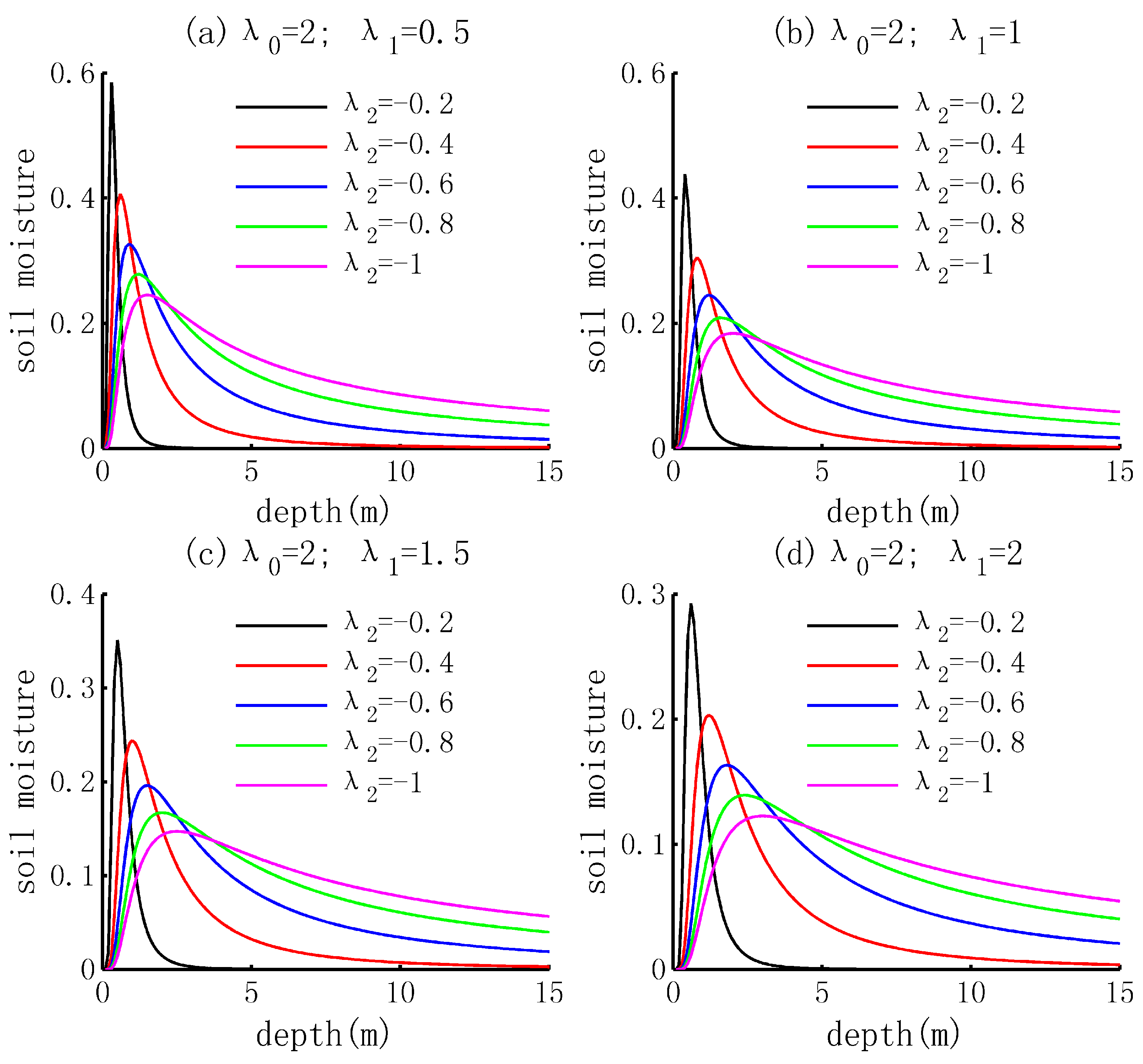
Equation (18) is the general form of a Gamma distribution. The soil moisture distribution based on a scaled PDF f(z)/C with different parameters is shown in Figure 3.

In the Badain Jaran Desert, one centimeter depth sand profile usually records the archive of the recharge from precipitation in a year [15]. In other words, the average flow rate of soil movement is 1 cm per year. This indicates the shape of the soil moisture profile is almost the constant at the scale of decades of years, so the geometric mean of the profile can be considered as a constant. Meanwhile the arithmetic mean can also be considered as constant since the average recharge rate is a constant at one thousand year scale. Hence, the two constricts, both constant in arithmetic mean and geometric mean, are reasonable to determine the soil moisture distribution in desert region at the scale of a couple of decade years. The PDF of gamma distribution also displays the same pattern as the soil moisture profiles in desert regions, as shown in Figure 3 and Figure 4, respectively.

5. Parameterization

Actually, the soil moisture distribution is measured at a limit depth, which would lead to a substantial difference of the parameters (both arithmetic mean and geometric mean) between the real value and estimated value by samples, especially for the soil moisture distribution displaying the trend of increase then being stable. Even worse, both arithmetic mean and geometric mean are difficult to obtain at the depth of 10 m without drilling samples. Fortunately, previous studies showed that soil moisture distribution is correlated to local environmental factors in this region [12,13]. Therefore we can estimate the parameters based on the local environmental factors through the application of fuzzy mathematics method. In this study, multilinear equations are used to determine the parameters of the scaled PDF of gamma distribution.

5.1. Soil Moisture Data

Nineteen random deep soil moisture profiles are used to test the simulated results. Sand samples were collected from the southeastern part of the Badain Jaran Desert where dunes and lakes are densely interspersed (Figure 2) in June 2005 and September 2007. Samples in the unsaturated zone were obtained to a depth of about 10 m using a 50 cm hollow-stem hand auger (Dormer Engineering, Murwillumbah, Australia) with interchangeable 1.5 m aluminum rods. Bulk sediment samples of approximately 500 g were collected at intervals of 0.25 m in top 3 m and 0.50 m in 3–10 m respectively. Samples were homogenized over the sampled interval and immediately sealed in polyethylene bags, care being taken to avoid moisture loss. Locations and elevations were recorded with a Garmin GPS, as shown in

Table 1. Local environmental factors of typical random soil moisture profiles.

ID	Depth	Relative Elev. (m)	Distance to Lake (m)	Dry Layers (cm)	Slope (°)	Orientation	Vegetation
DS	10.5	70	967	40	9	NW	Sparse
ES	10.5	25	1580	40	7	NW	Sparse
FS	10.5	176	1688	40	3	NW	Sparse
SA	13.5	18	251	40	5	NW	Sparse
SB	10	76	510	40	13	SE	Sparse
SC	10	24	513	60	0	SW	Sparse
SD	10	59	932	35	4	S	Very sparse
SE	10	22	944	40	6	NE	None
SF	10	32	2000	40	0	NE	Sparse to moderate
SH	10	21	1100	40	4	N-NW	Sparse
SJ	10	21	1400	40	5	SW	Sparse
SM	10	86	1600	40	0	NE	Sparse
SN	8.5	81	2600	30	12	NW	Very sparse
SO	10	21	1000	36	3	NW	Very sparse
SP	10	44	1300	23	8	NW	Sparse
SQ	8.65	44	1800	35	1	W-NW	Sparse
SU	9	32	354	45	1.5	W-NW	Sparse
SV	10	45	250	40	10	NW	Sparse to moderate
SW	10	39	500	40	0	SE	Very sparse

. Moisture contents were determined gravimetrically after drying overnight at 110 °C. These data have been partly reported in the previous studies [12,13,19,25,26,27].

5.2. Data Preparation for Multiple Linear Regressions

Before multiple linear regressions, the local terrain and vegetation data was encoded to qualify the data. For certain parameters, categories were more meaningful than the actual measured values. Thus, the slope orientation was encoded using eight equal 45 categories, moving clockwise from north (centered on an azimuth of 0, thus with azimuths for this initial category ranging from 337.5 to 22.5), following the method of Qiu and Zhang [17]. The sine of the half slope orientation was used to quantify its value as the sine increase from 0 to 90 degree and then decrease from 90 to 180 degree. Pulsing the constant 1 was used to calibrate quantity of orientation. The vegetation cover was classified into five categories: 0 represents none, 1 represents very sparse, 2 represents sparse, 3 represents sparse to moderate, and 4 represents moderate to relatively dense. The slope, relative elevation above the nearest lake, and distance to the nearest lake were measured at each sample site (Table 1). And the tangent value was used to quantify the slope of dunes. All environmental variables were normalized before the multiple regressions.

5.3. Solving Equations

The multiple regressions between the parameters of the scaled gamma PDF and local environmental factors are as follows:

(a)

Theoretical parameters. The theoretical value of the parameters of each profile is represented by values fitted using the least square fitting, denoted as Y.

(b)

The variables matrix are represented by the normalized environmental factors which were encoded by the specific rules mentioned above.

(c)

The coefficients or the weights of these environmental factors are obtained by solving by the linear equations.

With the exception of fitting by least squares, the weights of the environmental factors for the parameters of λ₀, λ₁, λ₂ are fitted by two methods: based on the environmental factors of all profiles (FAP) and leave itself out or the factors of the other profiles (FOP). The former use the same weight vector for all 19 profiles, while the latter need 19 vectors to determine the parameters for each profile, respectively. Here, we use the mean, standard deviation (STD) and coefficient of variance (CV) to describe these weights calculated by the second method, as shown in

Table 2. The weight of environmental factors for parameters of soil moisture distribution.

Para.	Fitting Method		Relative Elev. (m)	Dis. to Lake (m)	Dry Layers (cm)	Slope (°)	Orientation	Vegetation
λ0	FAP		0.0531	0.0475	0.0010	−0.1091	−0.1664	1.9491
		Average	0.0493	0.0441	0.0010	−0.1079	−0.1666	1.9502
	FOP	STD	0.0298	0.0435	0.0426	0.0290	0.0352	0.0331
		CV	0.6048	0.9849	−43.59	−0.2688	−0.211	0.017
λ1	FAP		0.0256	0.0091	−0.0115	0.0547	−0.0764	0.6018
		Average	0.0252	0.0070	−0.0137	0.0548	−0.0758	0.6021
	FOP	STD	0.0302	0.0258	0.0235	0.0129	0.0224	0.0196
		CV	1.2016	3.6881	−1.7105	0.2348	−0.2959	0.0326
λ2	FAP		−0.0218	0.0068	0.0155	−0.0203	0.0411	−0.1638
		Average	−0.0215	0.0076	0.0163	−0.0199	0.0405	−0.1639
	FOP	STD	0.0129	0.0112	0.0086	0.0048	0.0090	0.0082
		CV	−0.5980	1.4624	0.5260	−0.2426	0.2222	−0.0499

Notes: parameters are fitted by two ways, based on the environmental factors of all profiles (FAP) and factors of the other profiles (FOP).

. More details are listed in the Appendix (

Table A1. The weights of local environmental factors for parameter λ₀, represented by exp(λ₀−1).

ID	Relative Elevation (m)	Distance to Lake (m)	Dry Layers (cm)	Slope (°)	Orientation	Vegetation
FAP	0.0531	0.0475	0.0010	−0.1091	−0.1664	1.9491
SA	0.0520	−0.0102	0.0062	−0.1286	−0.2471	1.9979
SB	−0.0413	−0.0275	−0.0248	−0.1408	−0.1378	1.9069
SC	0.0181	0.0970	0.0195	−0.1220	−0.1801	1.9844
SD	0.0497	0.1112	−0.0308	−0.0938	−0.1626	1.9844
SE	0.0594	−0.0177	−0.1398	−0.1334	−0.1965	1.9986
SF	0.0058	0.0511	0.0882	−0.1595	−0.0796	1.9954
SH	0.0668	0.1236	−0.0033	−0.0714	−0.1533	1.9004
SJ	0.0343	−0.0373	−0.0299	−0.0591	−0.2287	1.9105
SM	0.0787	0.0587	−0.0007	−0.1286	−0.1701	1.9315
SN	0.0398	0.0460	0.0083	−0.1082	−0.1843	1.9418
SO	0.0778	0.0958	0.0609	−0.0831	−0.1498	1.9041
SP	0.0845	0.0313	0.0124	−0.1248	−0.1552	1.9871
SQ	0.0586	0.0444	−0.0017	−0.1058	−0.1757	1.9426
ST	0.0838	0.0628	−0.0050	−0.1118	−0.1182	1.9146
SU	0.0518	0.0482	−0.0007	−0.1093	−0.1646	1.9480
SW	0.0713	0.0313	0.0176	−0.1136	−0.1543	1.9335
DS	0.0546	0.0463	0.0013	−0.1081	−0.1675	1.9507
ES	0.0558	0.0466	0.0025	−0.1137	−0.1622	1.9529
FS	0.0316	0.0337	−0.0007	−0.0329	−0.1784	1.9689
Average	0.0493	0.0441	−0.0010	−0.1079	−0.1666	1.9502
STD	0.0298	0.0435	0.0426	0.0290	0.0352	0.0331
CV	0.6048	0.9849	−43.5917	−0.2688	−0.2110	0.0170

,

Table A2. The weight of local environmental factors for parameter λ₁.

ID	Relative Elevation (m)	Distance to Lake (m)	Dry Layers (cm)	Slope (°)	Orientation	Vegetation
FAP	0.0256	0.0091	−0.0115	0.0547	−0.0764	0.6018
SA	0.0253	−0.0051	−0.0103	0.0499	−0.0963	0.6139
SB	−0.0847	−0.0785	−0.0416	0.0177	−0.0430	0.5526
SC	−0.0010	0.0467	0.0025	0.0449	−0.0868	0.6286
SD	0.0243	0.0340	−0.0240	0.0607	−0.0749	0.6156
SE	0.0278	−0.0139	−0.0613	0.0461	−0.0871	0.6193
SF	0.0485	0.0074	−0.0538	0.0791	−0.1185	0.5794
SH	0.0258	0.0103	−0.0116	0.0553	−0.0762	0.6011
SJ	0.0260	0.0110	−0.0108	0.0536	−0.0750	0.6027
SM	0.0238	0.0083	−0.0114	0.0560	−0.0762	0.6030
SN	0.0750	0.0145	−0.0388	0.0510	−0.0100	0.6287
SO	0.0475	0.0520	0.0415	0.0778	−0.0617	0.5621
SP	0.0319	0.0058	−0.0092	0.0515	−0.0742	0.6096
SQ	0.0238	0.0101	−0.0107	0.0536	−0.0734	0.6039
ST	0.0264	0.0095	−0.0117	0.0546	−0.0751	0.6009
SU	0.0538	−0.0070	0.0249	0.0571	−0.1127	0.6237
SW	0.0383	−0.0022	0.0001	0.0516	−0.0680	0.5910
DS	0.0204	0.0129	−0.0125	0.0512	−0.0726	0.5962
ES	0.0249	0.0093	−0.0119	0.0558	−0.0775	0.6009
FS	0.0202	0.0057	−0.0120	0.0737	−0.0794	0.6068
Average	0.0252	0.0070	−0.0137	0.0548	−0.0758	0.6021
STD	0.0302	0.0258	0.0235	0.0129	0.0224	0.0196
CV	1.2016	3.6881	−1.7105	0.2348	−0.2959	0.0326

and

Table A3. The weight of local environmental factors for parameter λ₂.

ID	Relative Elevation (m)	Distance to Lake (m)	Dry Layers (cm)	Slope (°)	Orientation	Vegetation
FAP	0.0531	0.0475	0.0010	−0.1091	−0.1664	1.9491
SA	0.0520	−0.0102	0.0062	−0.1286	−0.2471	1.9979
SB	−0.0413	−0.0275	−0.0248	−0.1408	−0.1378	1.9069
SC	0.0181	0.0970	0.0195	−0.1220	−0.1801	1.9844
SD	0.0497	0.1112	−0.0308	−0.0938	−0.1626	1.9844
SE	0.0594	−0.0177	−0.1398	−0.1334	−0.1965	1.9986
SF	0.0058	0.0511	0.0882	−0.1595	−0.0796	1.9954
SH	0.0668	0.1236	−0.0033	−0.0714	−0.1533	1.9004
SJ	0.0343	−0.0373	−0.0299	−0.0591	−0.2287	1.9105
SM	0.0787	0.0587	−0.0007	−0.1286	−0.1701	1.9315
SN	0.0398	0.0460	0.0083	−0.1082	−0.1843	1.9418
SO	0.0778	0.0958	0.0609	−0.0831	−0.1498	1.9041
SP	0.0845	0.0313	0.0124	−0.1248	−0.1552	1.9871
SQ	0.0586	0.0444	−0.0017	−0.1058	−0.1757	1.9426
ST	0.0838	0.0628	−0.0050	−0.1118	−0.1182	1.9146
SU	0.0518	0.0482	−0.0007	−0.1093	−0.1646	1.9480
SW	0.0713	0.0313	0.0176	−0.1136	−0.1543	1.9335
DS	0.0546	0.0463	0.0013	−0.1081	−0.1675	1.9507
ES	0.0558	0.0466	0.0025	−0.1137	−0.1622	1.9529
FS	0.0316	0.0337	−0.0007	−0.0329	−0.1784	1.9689
Average	0.0493	0.0441	−0.0010	−0.1079	−0.1666	1.9502
STD	0.0298	0.0435	0.0426	0.0290	0.0352	0.0331
CV	0.6048	0.9849	−43.5917	−0.2688	−0.2110	0.0170

correspond to λ₀, λ₁, and λ₂, respectively).

By comparing the weight vectors estimated by the two method above, we find that, generally, there is little difference between weights estimated by all profiles and the mean of weights by leave itself out. However, a larger CV is observed in the factor of relative elevation, distance to lake and thickness of dry layer, which are the sensitive factors affecting the soil moisture distribution based on detrended canonical correspondence analysis (DCCA) [12,13]. When the weights of the environmental factors are determined, the parameters of soil moisture distribution can be calculated by the encoded environmental variable matrix multiplying the weight vectors listed in Table 2 and Table A1, Table A2 and Table A3.

Table 3. Parameters estimation of soil moisture distribution as a scaled PDF of gamma distribution through different fittings.

ID	Best Fitted			Fitted by All Profiles			Fitted by Other 18 Profiles
	Exp(λ0−1)	λ1	λ2	Exp(λ0−1)	λ1	λ2	Exp(λ0−1)	λ1	λ2
SA	1.52	0.47	−0.09	2.07	0.54	−0.13	2.20	0.55	−0.14
SB	2.61	1.24	−0.45	1.83	0.81	−0.22	1.31	0.53	−0.06
SC	1.69	0.24	0.01	2.06	0.65	−0.17	2.13	0.72	-0.19
SD	1.56	0.47	−0.10	1.93	0.50	−0.13	2.01	0.50	−0.14
SE	1.58	0.45	−0.14	1.72	0.50	−0.15	1.82	0.55	−0.15
SF	1.19	0.66	−0.09	1.79	0.82	−0.20	2.47	1.00	−0.34
SH	2.70	0.55	−0.21	2.20	0.54	−0.14	2.02	0.53	−0.11
SJ	2.53	0.53	−0.14	1.95	0.68	−0.19	1.83	0.71	−0.20
SM	1.89	0.54	−0.13	1.98	0.64	−0.19	2.16	0.82	−0.31
SN	1.60	0.30	−0.05	2.19	0.54	−0.14	2.36	0.61	−0.16
SO	2.69	1.17	−0.42	1.96	0.62	−0.17	1.84	0.53	−0.13
SP	1.29	0.45	−0.06	1.92	0.67	−0.19	2.07	0.72	−0.21
SQ	1.84	0.46	−0.12	1.69	0.45	−0.14	1.56	0.45	−0.15
ST	2.69	0.66	−0.21	2.01	0.53	−0.14	1.88	0.51	−0.12
SU	2.24	0.47	−0.15	1.85	0.59	−0.15	1.53	0.69	−0.16
SW	2.35	0.80	−0.20	2.22	0.50	−0.13	2.16	0.37	−0.09
DS	1.93	0.76	−0.20	1.97	0.58	−0.16	1.98	0.54	−0.15
ES	1.84	0.53	−0.18	1.84	0.63	−0.19	1.84	0.68	−0.20
FS	1.29	0.67	−0.19	1.84	0.65	−0.20	2.47	0.62	−0.22

presents parameters exp(λ₀−1), λ₁ and λ₂ fitted by the three methods mentioned above.

6. Simulation Results and Precision

6.1. Simulation Results

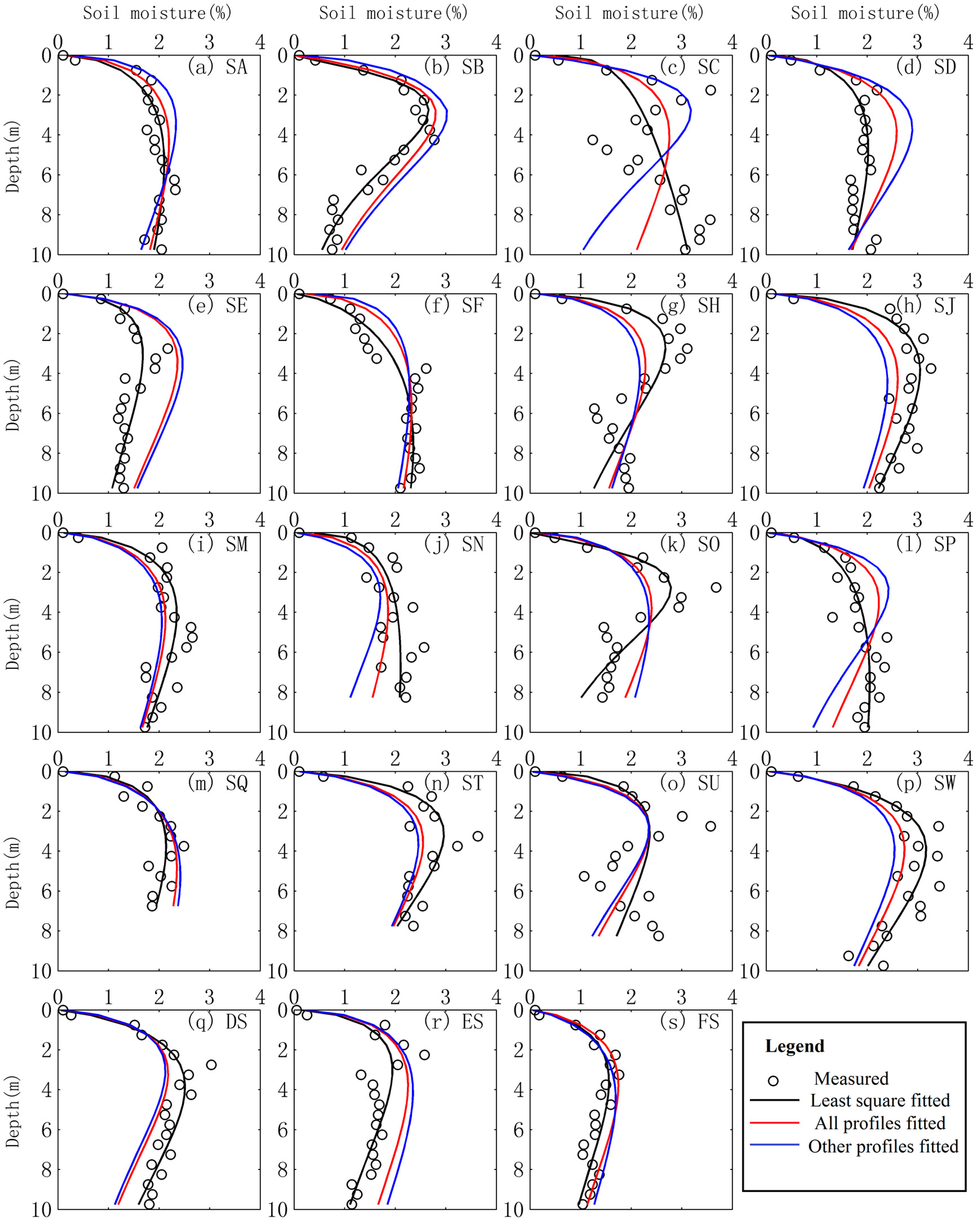
On the basis of the input parameters for each profile shown in Table 3, the soil moisture profiles are estimated by substituting these parameters into the scaled gamma distribution PDF. Figure 4 presents the measured data and the simulated results based on best fitted method, calibrating parameters using all profiles’ environmental factors and leaving itself out.

6.2. Correlation Analysis

Firstly, the correlation coefficients between measured data and simulated results are used to evaluate the performance of the entropy theory based model. The results are shown in

Table 4. Performance of the entropy based method under different fittings.

ID	Correlation Coefficient			Relative Error
	Best Fitted	By All Profiles	By Other 18 Profiles	Best Fitted		By All Profiles		By Other Profiles
				Mean	STD	Mean	STD	Mean	STD
SA	0.94	0.93	0.90	6.88%	6.31%	12.26%	11.36%	14.87%	12.93%
SB	0.97	0.95	0.93	13.69%	13.57%	18.53%	35.86%	23.14%	25.99%
SC	0.73	0.56	0.50	21.92%	25.24%	30.39%	27.82%	45.41%	31.23%
SD	0.91	0.87	0.83	9.43%	7.26%	23.08%	10.96%	28.53%	14.42%
SE	0.87	0.86	0.85	11.52%	7.65%	41.96%	20.70%	48.76%	21.80%
SF	0.94	0.90	0.85	9.92%	8.36%	14.83%	18.01%	16.83%	21.54%
SH	0.83	0.75	0.70	19.22%	17.73%	22.00%	16.64%	22.35%	16.12%
SJ	0.94	0.93	0.92	6.71%	6.23%	14.70%	7.99%	18.54%	9.04%
SM	0.91	0.90	0.90	10.12%	8.18%	12.25%	9.26%	12.06%	9.93%
SN	0.87	0.82	0.72	12.43%	8.51%	16.83%	10.04%	25.30%	14.91%
SO	0.90	0.76	0.68	17.89%	14.62%	27.99%	15.16%	28.86%	15.56%
SP	0.92	0.68	0.54	9.41%	10.47%	23.11%	14.82%	35.63%	17.13%
SQ	0.92	0.90	0.90	10.61%	9.23%	14.07%	11.09%	13.79%	11.94%
ST	0.91	0.90	0.90	10.61%	7.49%	13.97%	9.51%	12.90%	11.01%
SU	0.68	0.66	0.65	26.00%	25.54%	27.58%	21.25%	27.59%	19.77%
SW	0.95	0.94	0.94	9.03%	7.46%	12.78%	7.77%	17.82%	7.60%
DS	0.94	0.91	0.90	7.81%	5.24%	16.64%	9.84%	19.96%	10.62%
ES	0.84	0.80	0.77	12.62%	11.16%	30.13%	16.47%	39.92%	20.07%
FS	0.92	0.91	0.88	10.68%	6.13%	14.90%	12.81%	18.72%	25.81%

.

Theoretically, the best fitted results display a good linear correlation with the measured value. There are 13 profiles that show correlation coefficients larger than 0.9, four profiles between 0.8 and 0.9 and two profiles about 0.7. As for the profiles of SC and SU, the least correlation between the measured and best gamma PDF fitted result, both profiles exhibit a substantial change of sand texture: a higher clay content appearing when the soil moisture increases again. Therefore, these scaled PDF are appropriate for about ninety five percent of the soil moisture profiles in the deep vadose zone of the Badian Jaran Desert, and the two exceptions are caused by the change of sand texture.

The correlation coefficients of the fitted results on the basis of local environmental factors from all 19 profiles perform well too: ten profiles showing larger than 0.9, four profiles between 0.8 and 0.9, two profiles between 0.75 and 0.8, and three profiles between 0.56–0.75. The results based on other 18 profiles are mostly close to those based on all nineteen profiles. Eight profiles displays correlation coefficients larger than 0.9, four profiles between 0.8 and 0.9, five profiles are about 0.7 or higher, and two profiles (SC and SU) between 0.5 and 0.7. Hence, the simulated results display a good correlation with the measured values.

6.3. Error Analysis

Similarly, the results of error analysis are shown in Table 4 too. The relative error is used to quantify the performance of the simulated results. Firstly, the best fitted results display a small error between the simulated and measured values. The average relative errors are less than 0.15 in fifteen profiles, and four profiles are between 0.15 and 0.3. This indicates this method can provide good precision for most of the soil moisture profiles.

The fitted results based on local environmental factors also perform well. Most of the relative errors are less than 30% and the maximum average error is less than 50% in a profile, although several profiles showing a good correlation coefficients exhibit a high relative error, such as SE, SP and ES. In the top ten meter depth zone of desert regions, this precision is acceptable on the basis of local environmental factors instead of drilling samples and drying them.

By comparison the errors based on parameters estimated by two methods, we find the model performs a little better when parameters determined by all the profiles’ environmental factors than fitted by leave itself out. The reason is the former counts in the autocorrelation, and the latter is more objective as the validation is performed on data that were not used in the calibration. Hence, we concentrate more on discussing the errors from the second method and analyzing the main driving factors.

Generally, the performance of the model calibrated by the last method deliver an acceptable accuracy although the error might be close to 50% in a couple of profiles. Nine profiles show a high accuracy with errors less than 20%, six profiles showing a middle level with errors between 20% and 30%, and poor performance (30%–40%) is seen in four profiles, including SC, SE, SP and ES. From the estimated parameters of the profiles in which the model performs poorly, we can find that: (1) the reason for SC is the change of soil texture with more clay content that leads to the soil moisture pattern not be consistent with that of the gamma distribution; (2) SE, SP and ES, however, are able to show good precision when fitted appropriately; (3) profile SE exhibits a good CC but a large relative error. This means the parameters for λ₁ and λ₂ are estimated appropriately, while λ₀, the factor to scale the PDF, is higher than the real value; (4) as for ES, the middle level CC indicates the error is not caused by λ₀ alone, and actually the reason is mainly due to a larger λ₁ from Table 3; (5) finally, the estimated three parameters of SP are different from the best fitted value: a larger value for λ₀, λ₁, and smaller for λ₂. This means the estimated soil moisture concentrates more around the mode than the measured profile. Combined our previous studies based on detrended canonical correspondence analysis (DCCA), the dominating factor is thickness of the dry sand layer near the surface for SE and ES, and distance to lake for SP, respectively [12,13]. Compared with the other environmental factors, the thickness of the dry sand near the surface can be affected by small intensity precipitation, which might lead to the model performing poorly in some profiles. For SP, it is located near a lake that has dried up, and the measured distance is to another lake located beyond the divide line of the dried lake.

6.4. Applicability of the Model

This method performs well on estimating soil moisture distribution in most profiles with the exception of several profiles caused by abrupt change of texture, such as SC and SU, in the study area, the Badain Jaran Desert of northwestern China. In order to simulate the soil moisture profiles based on local land surface factors instead of sampling sand vertically, three requirements should be met.

The first is the soil moisture distribution can be considered as stable in a specific period. Here, the soil moisture distribution at the top ten meter zone of the desert region meets the first requirement since the soil water moves at a very low flow rate (about 1 cm/year) and the ten meter depth sand profile represents a one thousand year recharge record. The former indicates the shape of the soil moisture profile is almost a constant, so the geometric mean of the profile can be considered as a constant. The latter indicates that the arithmetic mean is a constant as the average recharge rate is a constant at a one thousand year scale. Hence, the two limitations, both constant in arithmetic mean and geometric mean, are necessary to determine patterns of soil moisture distribution.

The second requirement is a gradual change of soil texture and soil moisture. As presented in the text above, the abrupt change of texture will lead to the model performing poorly in these profiles like SC and SU. The reason is the trend of the PDF of the gamma distribution decreases monotonously after the mode. In the desert region, fortunately, most of the soil moisture profiles exhibit the same trend which enables the applicability of this method in the desert regions.

Another requirement is determining the weight vector of the environmental factors based on sufficient measured soil moisture profiles. In this study, nineteen soil moisture profiles are used to calibrate the parameters by the application of fuzzy mathematics. In a desert region, the influence of rainfall on soil moisture is mostly small in a short period, hence the relationships can be established simply by the linear equations.

In other regions, however, the soil moisture distribution is not static. For example, in humid climatic conditions, the vertical soil moisture distribution varies substantially on a daily scale or even an hourly scale. The reason is the much more intensive and frequent precipitation will lead to the temporal and spatial patterns of soil moisture varying substantially. On the contrary, the soil moisture distribution is determined mainly by the long term climatic conditions, and the precipitation events have little effect on soil moisture distribution in the deep vadose zone of desert regions at a daily or monthly scale. Therefore, the assumption of static state is appropriate for the arid desert regions while it is challenged in humid regions.

7. Conclusions

From the establishment of the model based on information entropy, parameter determination and precision tests, the conclusions of this work are as follows:

• The soil moisture distribution curve can be described as a scaled PDF in the deep vadose zone of the Badian Jaran Desert. The function is solved by PME with the constraint of normalization, known arithmetic mean and geometric mean, and the soil moisture vertical distribution curve is a scaled PDF of gamma distribution with a general form as $f(z)=e^{{\lambda }_0-1}{e}^{{\lambda }_{1}z}{z}^{{\lambda }_2}$.
• The parameters of soil moisture distribution are estimated by local land surface environmental factors like terrain and vegetation: the theoretic parameters are estimated by least squares fitting, then the linear equations were used to describe the relationship between environmental factors and best fitted parameters. The coefficients of the environmental factors are obtained by solving these equations.
• The simulated results show a good correlation and an acceptable precision with the measured values. The correlation coefficient is larger than 0.9 in more than a half profiles and most are over 0.8; the relative errors are smaller than 30% in most of the profiles and it can less than 15% when fitted by appropriate parameters.

Therefore, a simple alternative method is established to estimate the soil moisture distribution in the deep vadose zone of desert regions based on the local land surface environmental factors, and this method would be useful since these environmental factors can be obtained by remote sensing data. Meanwhile, we should bear in mind that this method is applicable in desert regions but challenged in humid and semi-humid regions. The reason is the former is determined mainly by the long term climatic conditions and local environmental factors, while the latter is determined by the short term climatic conditions, especially more intensive and frequent precipitation.

References

1. Western, A.W.; Grayson, R.B.; Blöschl, G.; Willgoose, G.R.; McMahon, T.A. Observed spatial organization of soil moisture and its relation to terrain indices. Water Resour. Res. 1999, 35, 797–810. [Google Scholar] [CrossRef]
2. Western, A.W.; Blöschl, G. On the spatial scaling of soil moisture. J. Hydrol. 1999, 217, 203–224. [Google Scholar] [CrossRef]
3. Eltahir, E.A. A soil moisture—Rainfall feedback mechanism: 1. Theory and observations. Water Resour. Res. 1998, 34, 765–776. [Google Scholar] [CrossRef]
4. Nash, J.E.; Sutcliffe, J.V. River flow forecasting through conceptual models part I, a discussion of principles. J. Hydrol. 1970, 10, 282–290. [Google Scholar] [CrossRef]
5. Nash, M.S.; Wierenga, P.J.; Gutjahr, A. Time series analysis of soil moisture and rainfall along a line transect in arid rangeland. Soil Sci. 1991, 152, 189–198. [Google Scholar] [CrossRef]
6. Ulaby, F.T.; Dubois, P.C.; van Zyl, J. Radar mapping of surface soil moisture. J. Hydrol. 1996, 184, 57–84. [Google Scholar] [CrossRef]
7. Pachepsky, Y.; Guber, A.; Jacques, D.; Simunek, J.; van Genuchten, M.T.; Nicholson, T.; Cady, R. Information content and complexity of simulated soil water fluxes. Geoderma 2006, 134, 253–266. [Google Scholar] [CrossRef]
8. Al-Hamdan, O.Z.; Cruise, J.F. Soil moisture profile development from surface observations by principle of maximum entropy. J. Hydrol. Eng. 2010, 15, 327–337. [Google Scholar] [CrossRef]
9. Singh, V.P. Entropy theory for derivation of infiltration equations. Water Resour. Res. 2010, 46, W03527. [Google Scholar] [CrossRef]
10. Singh, V.P. Entropy theory for movement of moisture in soils. Water Resour. Res. 2010, 46, W03516. [Google Scholar] [CrossRef]
11. Mishra, V.; Ellenburg, W.L.; Al-Hamdan, O.Z.; Bruce, J.; Cruise, J.F. Modeling Soil Moisture Profiles in Irrigated Fields by the Principle of Maximum Entropy. Entropy 2015, 17, 4454–4484. [Google Scholar] [CrossRef]
12. Ma, J.Z.; Zhou, X.Y.; Wang, Y.Q.; Gates, J.B. Spatial distribution of soil moisture at unsaturated zone in megadunes, southeast of Badain Jaran Desert. J. Desert Res. 2011, 31, 1365–1372. [Google Scholar]
13. Pan, F.; Ma, J.; Zhou, X.; Edmunds, W.M.; Gates, J.B. Erratum to: Geostatistical characterization of soil moisture and chloride distribution in deep vadose profiles of the Badain Jaran Desert, Northwestern China. Environ. Earth Sci. 2013, 70, 2423. [Google Scholar] [CrossRef]
14. Cook, P.G.; Edmunds, W.M.; Gaye, C.B. Estimating paleorecharge and paleoclimate from unsaturated zone profiles. Water Resour. Res. 1992, 28, 2721–2731. [Google Scholar] [CrossRef]
15. Edmunds, W.; Tyler, S. Unsaturated zones as archives of past climates: toward a new proxy for continental regions. Hydrogeol. J. 2002, 10, 216–228. [Google Scholar] [CrossRef]
16. Ma, J.; Li, D.; Zhang, J.; Edmunds, W.M.; Prudhomme, C. Groundwater recharge and climatic change during the last 1000 years from unsaturated zone of SE Badain Jaran Desert. Chin. Sci. Bull. 2003, 48, 1469–1474. [Google Scholar] [CrossRef]
17. Qiu, Y.; Zhang, J. The ordination axes clustering based on detrended canonical correspondence analysis ordination and its application to the analysis of the ecological gradients of plant communities in Bashuigou catchment, Guandi Mountain. Acta Ecol. Sin. 2000, 20, 199–206. [Google Scholar]
18. Yan, M.C.; Wang, G.Q.; Li, B.S.; Dong, G.R. Formation and growth of high megadunes in Badain Jaran Desert. Acta. Geogr. Sin. 2001, 56, 83–91. [Google Scholar]
19. Ma, J.; Edmunds, W.M. Groundwater and lake evolution in the Badain Jaran Desert ecosystem, Inner Mongolia. Hydrogeol. J. 2006, 14, 1231–1243. [Google Scholar] [CrossRef]
20. Domrös, M.; P’eng, G. The Climate of China; Springer-Verlag: Berlin, Germany, 1988. [Google Scholar]
21. Shannon, C.E. A mathematical theory of communications, I and II, Bell Syst. Tech. J. 1948, 27, 379–423. [Google Scholar]
22. Jaynes, E.T. Information theory and statistical mechanics. II. Phys. Rev. 1957, 108, 171–190. [Google Scholar] [CrossRef]
23. Jaynes, E.T. Information theory and statistical mechanics. Phys. Rev. 1957, 106, 620–630. [Google Scholar] [CrossRef]
24. Conrad, K. Probability Distributions and Maximum Entropy. Available online: http://www.math.uconn.edu/~kconrad/blurbs/analysis/entropypost.pdf (accessed on 27 August 2016).
25. Gates, J.B.; Edmunds, W.M.; Darling, W.G.; Ma, J.; Pang, Z.; Young, A.A. Conceptual model of recharge to southeastern Badain Jaran Desert groundwater and lakes from environmental tracers. Appl. Geochem. 2008, 23, 3519–3534. [Google Scholar] [CrossRef] [Green Version]
26. Ma, J.; Edmunds, W.M.; He, J.; Jia, B. A 2000 year geochemical record of palaeoclimate and hydrology derived from dune sand moisture. Paleogeogr. Palaeoclimatol. Palaeoecol. 2009, 276, 38–46. [Google Scholar] [CrossRef]
27. Ma, J.; Wang, Y.; Zhao, X.; Jin, X.; Ning, N.; Edmunds, W.M.; Zhou, X. Spatial distribution of chloride and nitrate within an unsaturated dune sand of a cold-arid desert: Implications for paleoenvironmental records. Catena 2012, 96, 68–75. [Google Scholar] [CrossRef]
Figure 1. Illustration of moisture distributions in vadose zone (a) soil moisture profiles in shallow vadose zone [10]; (b) soil moisture profiles in deep vadose zone of Badain Jaran Desert [12].
Entropy 18 00323 g001
Figure 2. Location of the study area and spatial distribution of the sampling sites. Site 1, Wulanjilin; Site 2, Nuoertu; Site 3, Sayinwusu; Site 4, Baoritaolegai. The remote sense image is from Google earth, and the projection is WGS-1984 for the coordinates of sampling sites to keep the consistent with the Google earth.
Entropy 18 00323 g002
Figure 3. Illustration of soil moisture distribution based on a scaled PDF solved by PME with the constraints of normalization, known arithmetic mean and known geometric mean.
Entropy 18 00323 g003
Figure 4. Measured and simulated soil moisture distributions in deep vadose zone of the Badain Jaran Desert. Cycles are the measured soil moisture content, black line is fitted by least square, red line is fitted by all 19 profiles and blue lines is fitted by the other 18 profiles.
Entropy 18 00323 g004