
Differentiating Interictal and Ictal States in Childhood Absence Epilepsy through Permutation Rényi Entropy

Abstract
:1. Introduction
2. Methodology
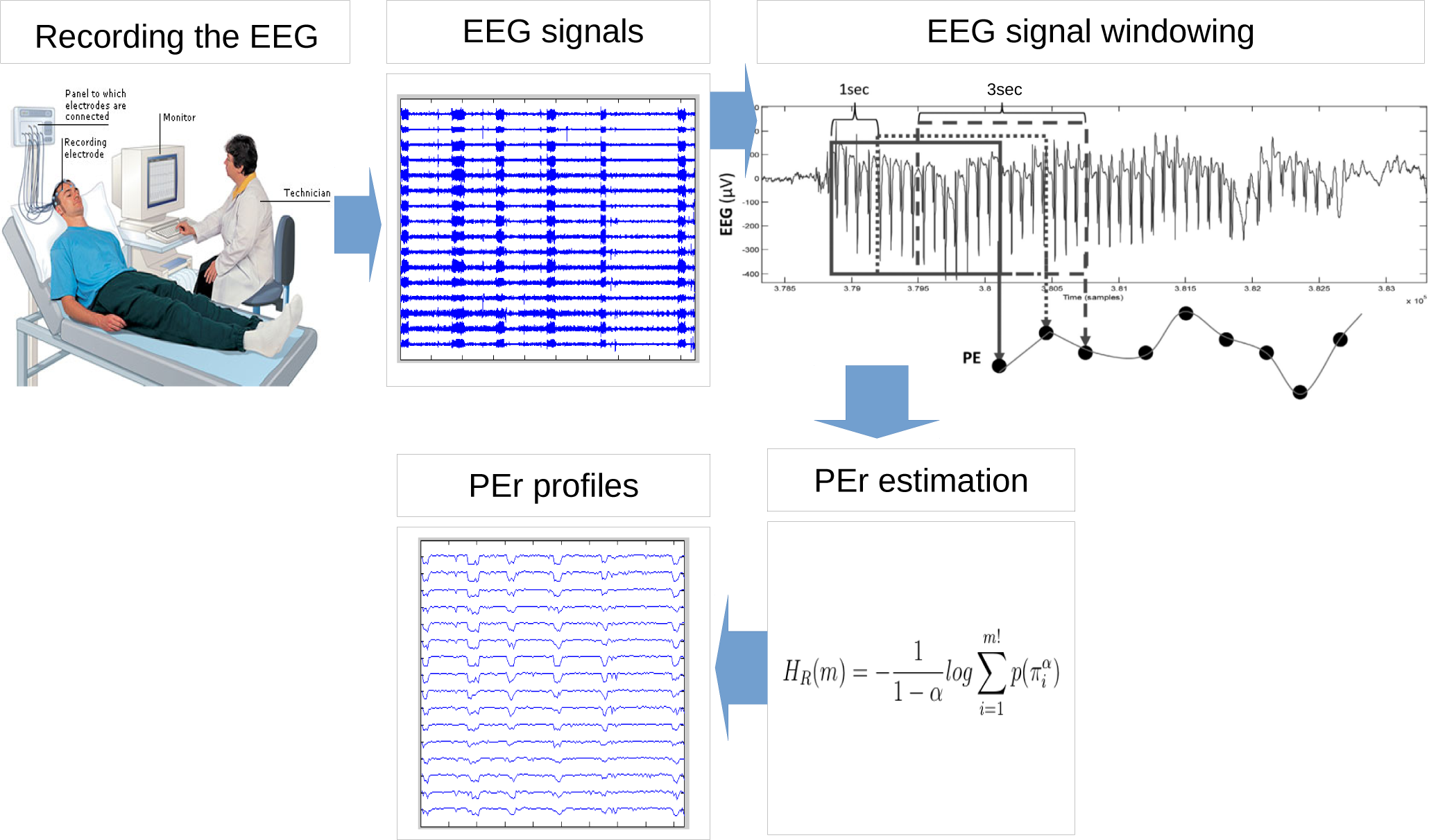
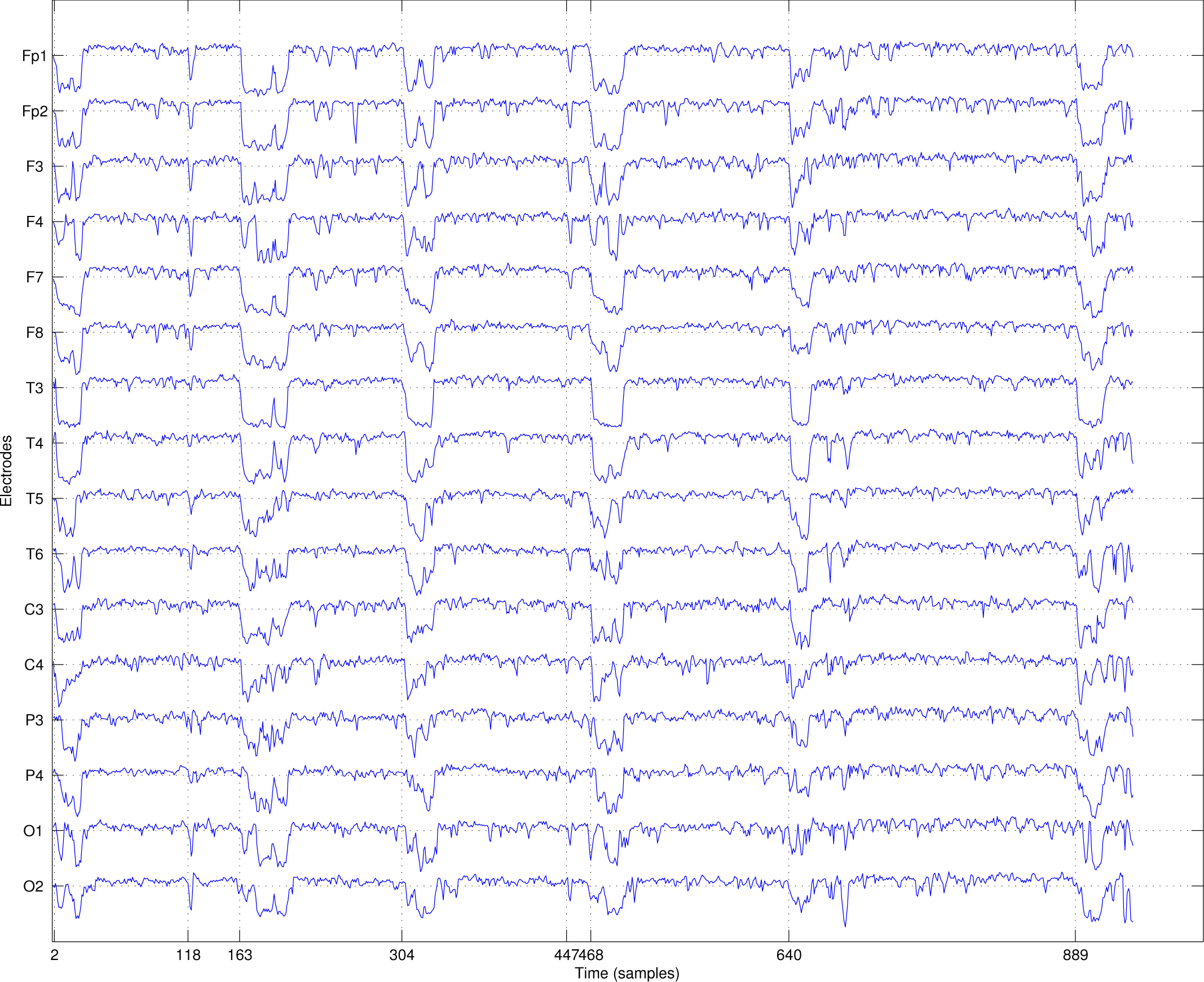
2.1. EEG Recording
2.2. Permutation Rényi Entropy
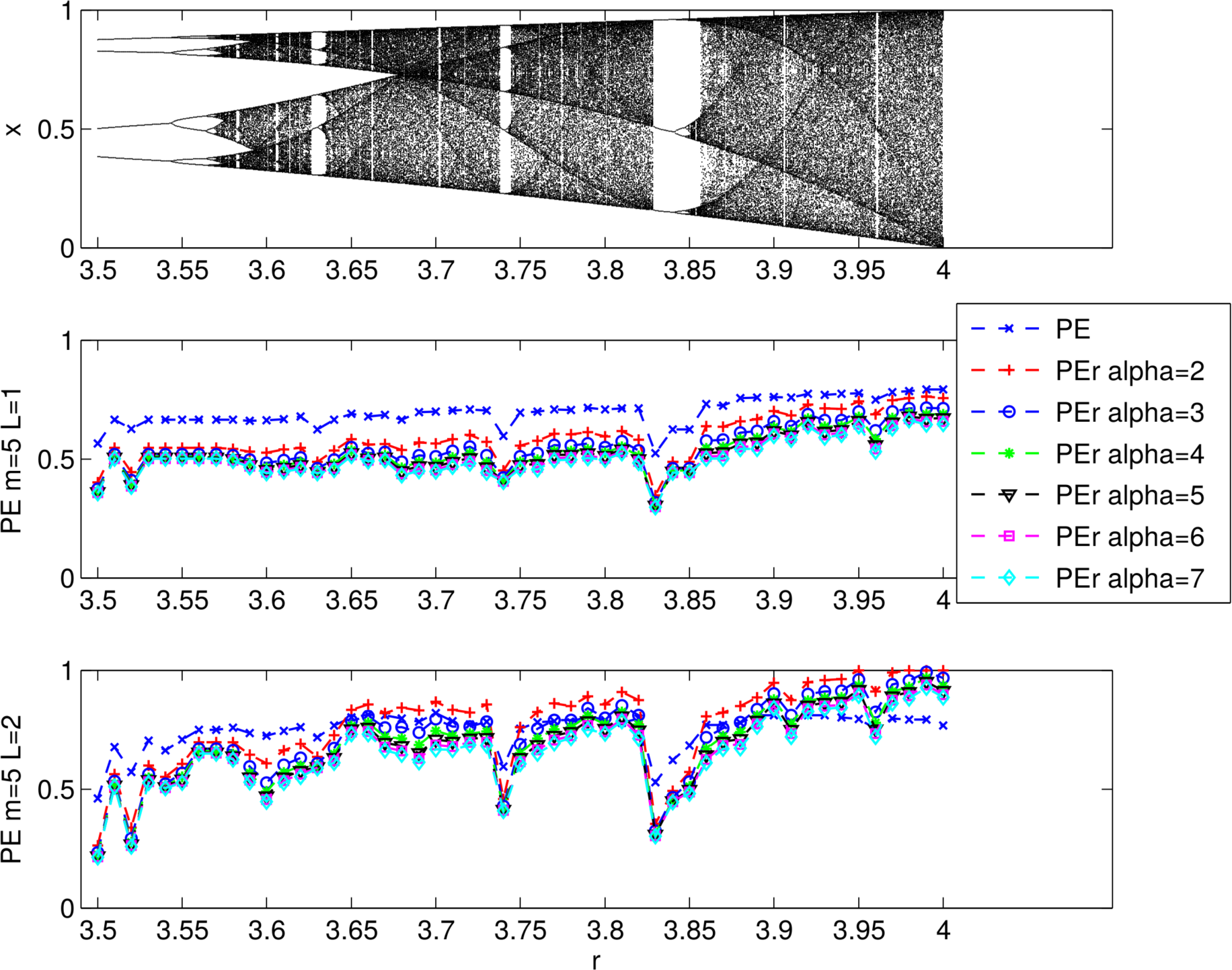
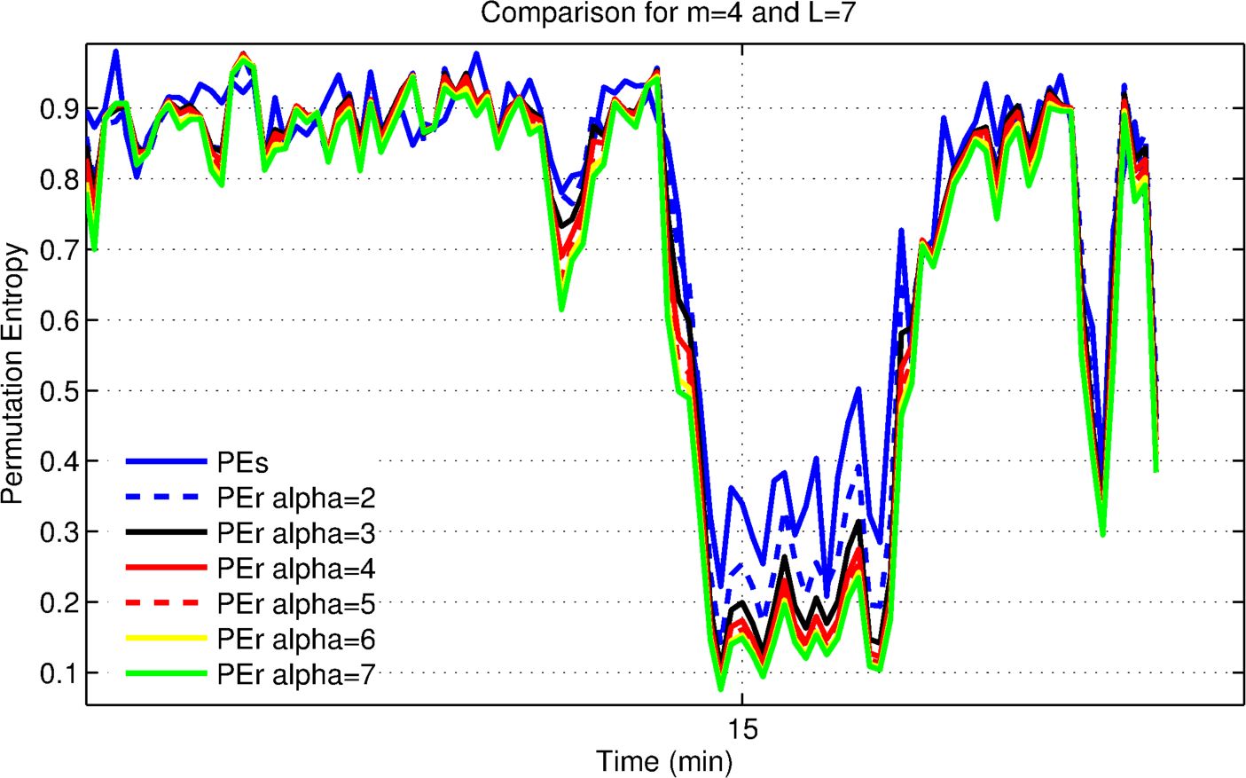
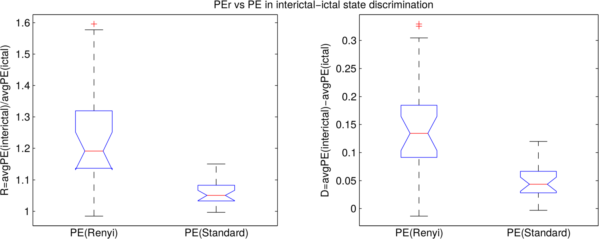
2.2.1. PEr vs. PE
2.2.2. Selecting the Optimal Parameter Configuration for PEr
- Order m ranging from 3–7;
- Lag L ranging from 1–10;
- α ranging from 2–7 (for PEr only).
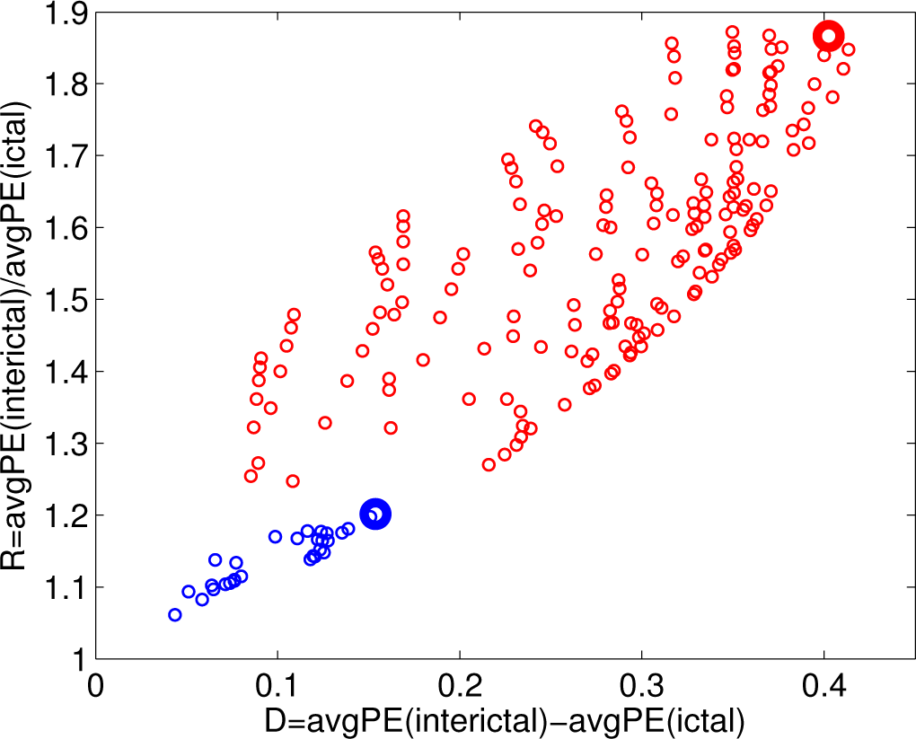
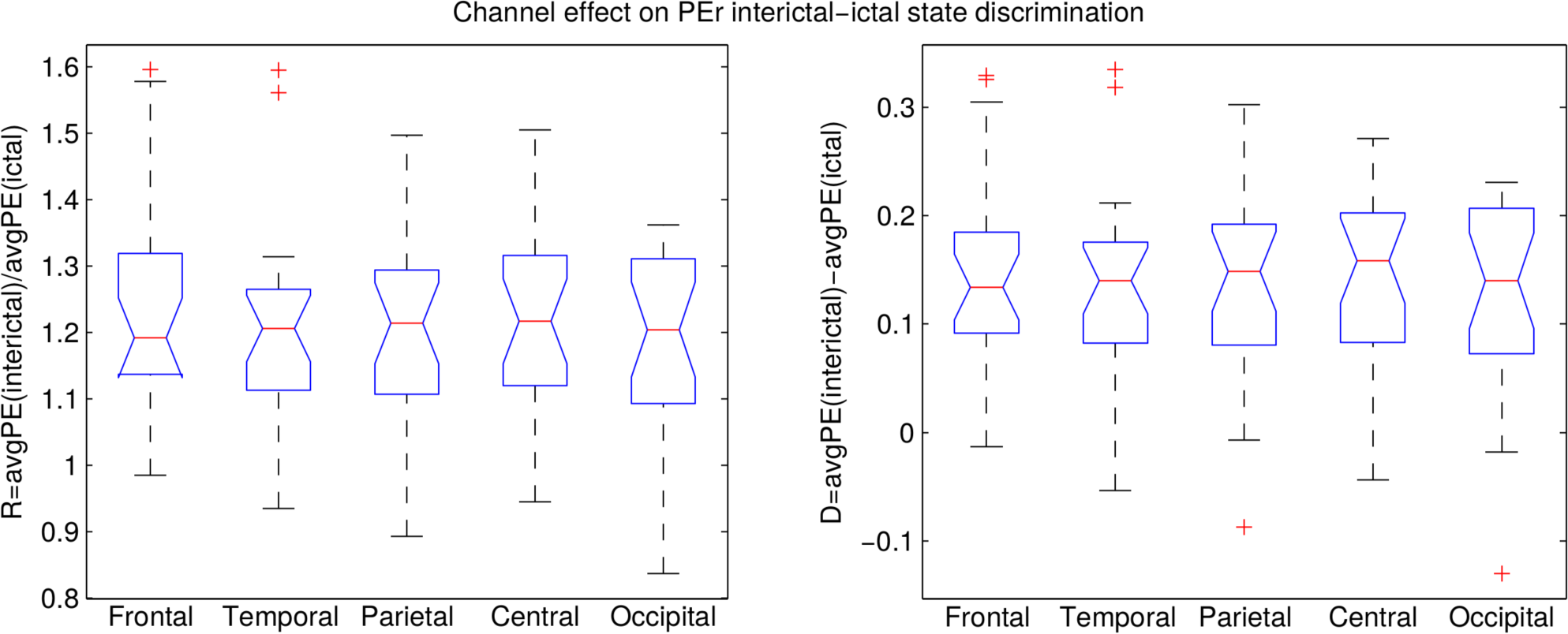
- the difference D = avgPE(interictal) − avgPE(ictal);
- the ratio R = avgPE(interictal)/avgPE(ictal).
3. Results
3.1. Analysis for Patient 4: Pilot Trial
3.1.1. Optimization for Patient 4
3.1.2. Evaluating the Effects of Alpha
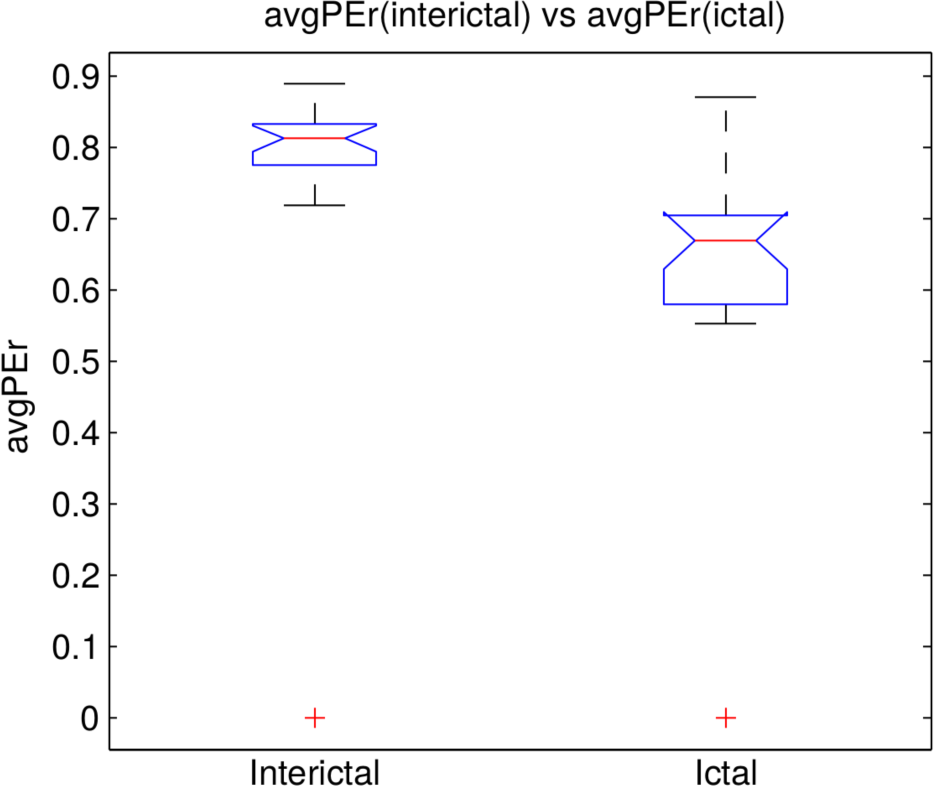
3.2. Analysis of the Entire Dataset
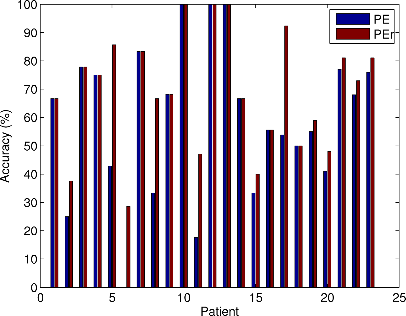
3.3. Classifying the Brain States according to PE and PEr
4. Conclusions
Acknowledgments
Appendix
A. Statistical Analysis
A.1. DPEr is Higher than DPE
A.2. RPEr is Higher than RPE
Author Contributions
Conflicts of Interest
References
- Duun-Henriksen, J.; Madsen, R.E.; Remvig, L.S.; Thomsen, C.E.; Sorensen, H.B.; Kjaer, T.W. Automatic detection of childhood absence epilepsy seizures: Toward a monitoring device. Pediatr. Neurol. 2012, 46, 287–292. [Google Scholar]
- Duun-Henriksen, J.; Kjaer, T.W.; Madsen, R.E.; Remvig, L.S.; Thomsen, C.E.; Sorensen, H.B. Channel selection for automatic seizure detection. Clin. Neurophysiol. 2012, 123, 84–92. [Google Scholar]
- Bandt, C.; Pompe, B. Permutation entropy: A natural complexity measure for time series. Phys. Rev. Lett. 2002, 88, 174102. [Google Scholar]
- Cao, Y.; Tung, W.-w.; Gao, J.B.; Protopopescu, V.A.; Hively, L.M. Detecting dynamical changes in time series using the permutation entropy. Phys. Rev. E 2004, 70, 046217. [Google Scholar]
- Li, X.; Ouyang, G.; Douglas, A.R. Predictability analysis of absence seizures with permutation entropy. Epilepsy Research. 2007, 77, 70–74. [Google Scholar]
- Bruzzo, A.A.; Gesierich, B.; Santi, M.; Tassinari, C.A.; Birbaumer, N.; Rubboli, G. Permutation entropy to detect vigilance changes and preictal states from scalp EEG in epileptic patients. a preliminary study. Neurol Sci. 2008, 29, 3–9. [Google Scholar]
- Zanin, M.; Zunino, L.; Rosso, O.A.; Papo, D. Permutation entropy and its main biomedical and econophysics applications: A review. Entropy 2012, 14, 1553–1577. [Google Scholar]
- Nicolaou, N.; Georgiou, J. Detection of epileptic electroencephalogram based on permutation entropy and support vector machines. Expert Syst. Appl. 2012, 39, 202–209. [Google Scholar]
- Ouyang, G.; Li, J.; Liu, X.; Li, X. Dynamic characteristics of absence EEG recordings with multiscale permutation entropy analysis. Epilepsy Res. 2013, 104, 246–252. [Google Scholar]
- Zhu, G.; Li, Y.; Wen, P.P.; Wang, S. Xi Epileptogenic focus detection in intracranial EEG based on delay permutation entropy. Proceedings of 2013 International Symposium on Computational Models for Life Sciences (CMLS 2013), Sydney, Australia, 27–29 November 2013; pp. 31–36.
- Zhu, G.; Li, Y.; Wen, P.P.; Wang, S. Classifying epileptic EEG signals with delay permutation entropy and multi-scale k-means. Adv. Exp. Med. Biol. 2015, 823, 143–157. [Google Scholar]
- Mateos, D.; Diaz, J.M.; Lamberti, P.W. Permutation entropy applied to the characterization of the clinical evolution of epileptic patients under pharmacological treatment. Entropy 2014, 16, 5668–5676. [Google Scholar]
- Li, J.; Liu, X.; Ouyang, G. Using relevance feedback to distinguish the changes in EEG during different absence seizure phases. Clin. EEG Neurosci. 2014. [Google Scholar] [CrossRef]
- Yang, Z.; Wang, Y.; Ouyang, G. Adaptive neuro-fuzzy inference system for classification of background EEG signals from eses patients and controls. Sci. World J 2014, 2014, 140863. [Google Scholar]
- Silva, A.; Ferreira, D.A.; Venâncio, C.; Souza, A.P.; Antunes, L.M. Performance of electroencephalogram-derived parameters in prediction of depth of anaesthesia in a rabbit model. Br. J. Anaesth. 2011, 106, 540–547. [Google Scholar]
- Li, D.; Li, X.; Liang, Z.; Voss, L.J.; Sleigh, J.W. Multiscale permutation entropy analysis of EEG recordings during sevoflurane anesthesia. J. Neural Eng. 2010, 7, 046010. [Google Scholar]
- Anier, A.; Lipping, T.; Jantti, V.; Puumala, P.; Huotari, A.M. Entropy of the EEG in transition to burst suppression in deep anesthesia: Surrogate analysis. Proceedings of 32nd Annual International Conference on IEEE Engineering in Medicine and Biology Society (EMBC), Buenos Aires, Argentina, 1–4 September 2010; pp. 2790–2793.
- Olofsen, E.; Sleigh, J.W.; DahanïijŇ, A. Permutation entropy of the electroencephalogram: a measure of anesthetic drug effect. Br. J. Anaesth. 2008, 101, 810–821. [Google Scholar]
- Li, D.; Liang, Z.; Wang, Y.; Hagihira, S.; Sleigh, J.W.; Li, X. Parameter selection in permutation entropy for an electroencephalographic measure of isoflurane anesthetic drug effect. J. Clin. Monit. Comput. 2013, 27, 113–123. [Google Scholar]
- Mammone, N.; Morabito, F.C.; Principe, J.C. Visualization of the short term maximum lyapunov exponent topography in the epileptic brain. Proceedings of 28th Annual International Conference on IEEE Engineering in Medicine and Biology Society (EMBC), New York City, NY, USA, 31 August–3 September 2006; pp. 4257–4260.
- Mammone, N.; Principe, J.C.; Morabito, F.C.; Shiau, D.S.; Sackellares, J.C. Visualization and modelling of stlmax topographic brain activity maps. J. Neurosci. Methods. 2010, 189, 281–294. [Google Scholar]
- Mammone, N.; Morabito, F.C. Analysis of absence seizure EEG via permutation entropy spatio-temporal clustering. Proceedings of the 2011 International Joint Conference on Neural Networks (IJCNN), San Jose, CA, USA, 31 July–5 August 2011; pp. 1417–1422.
- Mammone, N.; Labate, D.; Lay-Ekuakille, A.; Morabito, F.C. Analysis of absence seizure generation using EEG spatial-temporal regularity measures. Int. J. Neural Syst. 2012, 22, 1250024. [Google Scholar]
- Ferlazzo, E.; Mammone, N.; Cianci, V.; Gasparini, S.; Gambardella, A.; Labate, A.; Latella, M.A.; Sofia, V.; Elia, M.; Morabito, F.C.; Aguglia, U. Permutation entropy of scalp EEG: A tool to investigate epilepsies: Suggestions from absence epilepsies. Clin. Neurophysiol. 2014, 125, 13–20. [Google Scholar]
- Zhao, X.; Shang, P.; Huang, J. Permutation complexity and dependence measures of time series. Europhys. Lett. 2013, 102, 40005. [Google Scholar]
- Liang, Z.; Wang, Y.; Sun, X.; Li, D.; Voss, L.J.; Sleigh, J.W.; Hagihira, S.; Li, X. EEG entropy measures in anesthesia. Front. Comput. Neurosci. 2015, 9. [Google Scholar] [CrossRef]
- Malmivuo, J.; Plonsey, R. Bioelectromagnetism—Principles and Applications of Bioelectric and Biomagnetic Fields; Oxford University Press: New York, NY, USA, 1995. [Google Scholar]
- Kohonen, T. Learning vector quantization. In The Handbook of Brain Theory and Neural Networks; MIT Press: Cambridge, MA, USA, 1995; pp. 537–540. [Google Scholar]
- Shapiro, S.S.; Wilk, M.B. An analysis of variance test for normality (complete samples). Biometrika 1965, 52, 591–611. [Google Scholar]
- Mann, H.B.; Whitney, D.R. On a test of whether one of two random variables is stochastically larger than the other. Ann. Math. Stat. 1947, 18, 50–60. [Google Scholar]


| Pt | PE | PEr | |||
|---|---|---|---|---|---|
| m | L | m | L | α | |
| 1 | 4 | 3 | 5 | 4 | 6 |
| 2 | 4 | 2 | 5 | 3 | 3 |
| 3 | 4 | 10 | 4 | 7 | 7 |
| 4 | 4 | 8 | 4 | 7 | 7 |
| 5 | 3 | 10 | 3 | 5 | 7 |
| 6 | 4 | 3 | 5 | 5 | 7 |
| 7 | 4 | 2 | 5 | 3 | 7 |
| 8 | 4 | 10 | 5 | 4 | 7 |
| 9 | 4 | 3 | 5 | 6 | 7 |
| 10 | 4 | 3 | 5 | 5 | 6 |
| 11 | 4 | 3 | 4 | 3 | 5 |
| 12 | 4 | 3 | 5 | 5 | 5 |
| 13 | 4 | 8 | 4 | 7 | 7 |
| 14 | 4 | 3 | 5 | 4 | 7 |
| 15 | 4 | 2 | 4 | 3 | 4 |
| 16 | 4 | 3 | 5 | 4 | 6 |
| 17 | 5 | 3 | 4 | 6 | 7 |
| 18 | 4 | 2 | 4 | 2 | 2 |
| 19 | 4 | 3 | 5 | 4 | 6 |
| 20 | 4 | 3 | 4 | 3 | 4 |
| 21 | 4 | 3 | 5 | 5 | 6 |
| 22 | 4 | 3 | 5 | 3 | 4 |
| 23 | 4 | 3 | 4 | 7 | 7 |
© 2015 by the authors; licensee MDPI, Basel, Switzerland This article is an open access article distributed under the terms and conditions of the Creative Commons Attribution license (http://creativecommons.org/licenses/by/4.0/).
Share and Cite
Mammone, N.; Duun-Henriksen, J.; Kjaer, T.W.; Morabito, F.C. Differentiating Interictal and Ictal States in Childhood Absence Epilepsy through Permutation Rényi Entropy. Entropy 2015, 17, 4627-4643. https://doi.org/10.3390/e17074627
Mammone N, Duun-Henriksen J, Kjaer TW, Morabito FC. Differentiating Interictal and Ictal States in Childhood Absence Epilepsy through Permutation Rényi Entropy. Entropy. 2015; 17(7):4627-4643. https://doi.org/10.3390/e17074627
Chicago/Turabian StyleMammone, Nadia, Jonas Duun-Henriksen, Troels W. Kjaer, and Francesco C. Morabito. 2015. "Differentiating Interictal and Ictal States in Childhood Absence Epilepsy through Permutation Rényi Entropy" Entropy 17, no. 7: 4627-4643. https://doi.org/10.3390/e17074627