Article

High Recharge Areas in the Choushui River Alluvial Fan (Taiwan) Assessed from Recharge Potential Analysis and Average Storage Variation Indexes

1
Department of Civil Engineering, National Chiao-Tung University, No. 1001, University Road, Hsinchu City 30010, Taiwan
2
School of Environmental Studies, China University of Geosciences, Wuhan 430074, China
*
Author to whom correspondence should be addressed.
Entropy 2015, 17(4), 1558-1580; https://doi.org/10.3390/e17041558
Submission received: 22 May 2014 / Revised: 9 March 2015 / Accepted: 16 March 2015 / Published: 24 March 2015
(This article belongs to the Special Issue Entropy and Space-Time Analysis in Environment and Health)

Abstract

:
High recharge areas significantly influence the groundwater quality and quantity in regional groundwater systems. Many studies have applied recharge potential analysis (RPA) to estimate groundwater recharge potential (GRP) and have delineated high recharge areas based on the estimated GRP. However, most of these studies define the RPA parameters with supposition, and this represents a major source of uncertainty for applying RPA. To objectively define the RPA parameter values without supposition, this study proposes a systematic method based on the theory of parameter identification. A surrogate variable, namely the average storage variation (ASV) index, is developed to calibrate the RPA parameters, because of the lack of direct GRP observations. The study results show that the correlations between the ASV indexes and computed GRP values improved from 0.67 before calibration to 0.85 after calibration, thus indicating that the calibrated RPA parameters represent the recharge characteristics of the study area well; these data also highlight how defining the RPA parameters with ASV indexes can help to improve the accuracy. The calibrated RPA parameters were used to estimate the GRP distribution of the study area, and the GRP values were graded into five levels. High and excellent level areas are defined as high recharge areas, which composed 7.92% of the study area. Overall, this study demonstrates that the developed approach can objectively define the RPA parameters and high recharge areas of the Choushui River alluvial fan, and the results should serve as valuable references for the Taiwanese government in their efforts to conserve the groundwater quality and quantity of the study area.

1. Introduction

Delineating high groundwater recharge areas is a crucial step for sustainable groundwater resource management. An area with high recharge significantly influences the water quantity and quality of the regional groundwater system; while this can be beneficial in terms of water quantity, the infiltration process usually affects the transport of soil contaminations, and this can adversely impact the groundwater quality. Therefore, appropriate land use management practices in high recharge areas are important for groundwater conservation. Nevertheless, high groundwater recharge areas must be identified before applying any best management practices.
Many approaches have been proposed to identify high groundwater recharge areas [19]. The majority of these studies applied recharge potential analysis (RPA) to calculate index values representing the groundwater recharge potential (GRP), which is an indicator of the likelihood of surface water infiltrating all layers into an aquifer [10]. Specifically, high recharge areas were identified by using the estimated GRP values.
Defining the contributing factors related to groundwater recharge is the first step for determining GRP values. The contributing factors are selected according to the study area’s hydrology, geology, climate and human activities; such factors may include the lithology, drainage patterns, land use, land cover, precipitation, and so forth. Each contributing factor contains several attributes. For example, land use may contain wood land, grass land, farm, river, etc. Once defined, a geographic information system (GIS) map is developed for each contributing factor based on its original attributes. Second, the contributing factor’s original attribute values are mapped into score values according to their contribution to the groundwater recharge. Third, weights among the contributing factors are assigned, and the GRP values are acquired by summarizing the weighted scores of the contributing factors. Most studies summarize the contributing factor scores by applying GIS spatial analysis techniques.
The contributing factors adopted in RPA can be classified into two groups [1,39,11,12]. The first group contains the factors associated with the recharge source, such as precipitation, drainage, etc. The second group contains the factors influencing the infiltration, such as lithology, land use, land cover, slope, surface soil, geology, lineament, permeability, etc.
The RPA method has been applied to identify the GRP in many different environments [3,4,8,9,13]. However, the weight of each contributing factor and the mapping of the attributes to score values in previous studies were subjectively assigned. Defining the weights and the mappings without objective measures is a major source of uncertainty for applying the RPA method. Therefore, this study proposes a systematic approach to define the weights and mappings based on parameter identification. The GRP values can represent the potential for groundwater recharge. However, GRP lacks direct observations. Therefore, the identification of a surrogate variable of GRP to evaluate the correctness of RPA parameters, the weights and the mappings is essential.
Head changes are highly correlated with groundwater recharge, and these were selected to develop average storage variation (ASV) indexes to be used as the surrogate variable for GRP in this study. Yu and Chu [14,15] applied empirical orthogonal functions (EOF) to analyze the mechanisms that affect the spatiotemporal distribution of hydraulic heads in Taiwan’s Choushui River alluvial fan. These studies indicated that surface water infiltration is an important mechanism that affects the groundwater system of this alluvial fan; in particular, the first, third and fourth EOF were highly correlated with rainfall and stream flow, and these could explain about 70% of the observed spatiotemporal changes of head. Observed head changes highly correlated with surface water infiltration can be thought of as the consequence of groundwater recharge.
Beside groundwater recharge, head changes are also affected by aquifer storage capability. The aquifer storage capability represents the amount of ground void space that can store water, and it is usually represented by the specific yield (Sy) and storage coefficient (Sc), which depend on the unconfined and confined aquifer types, respectively. The head changes are more significant in an aquifer with low Sy/Sc than those in an aquifer with high Sy/Sc. To objectively define the reference indexes to be the surrogate variable of GRP, both head changes and aquifer storage capability were used to develop the ASV indexes, which represent the average storage variation of an aquifer.
To objectively and accurately estimate the high recharge areas of the study area, this study proposes a methodology to identify the RPA parameters based on the developed ASV indexes. First, the RPA is developed to estimate the GRP of the study area, and four contributing factors (land use, surface soil texture, average annual rainfall and drainage density) are considered in this analysis. Next, the RPA parameters are calibrated based on the ASV indexes. Finally, the groundwater recharge areas of Taiwan’s Choushui River alluvial fan are estimated using the developed GRP map.

2. Materials and Methods
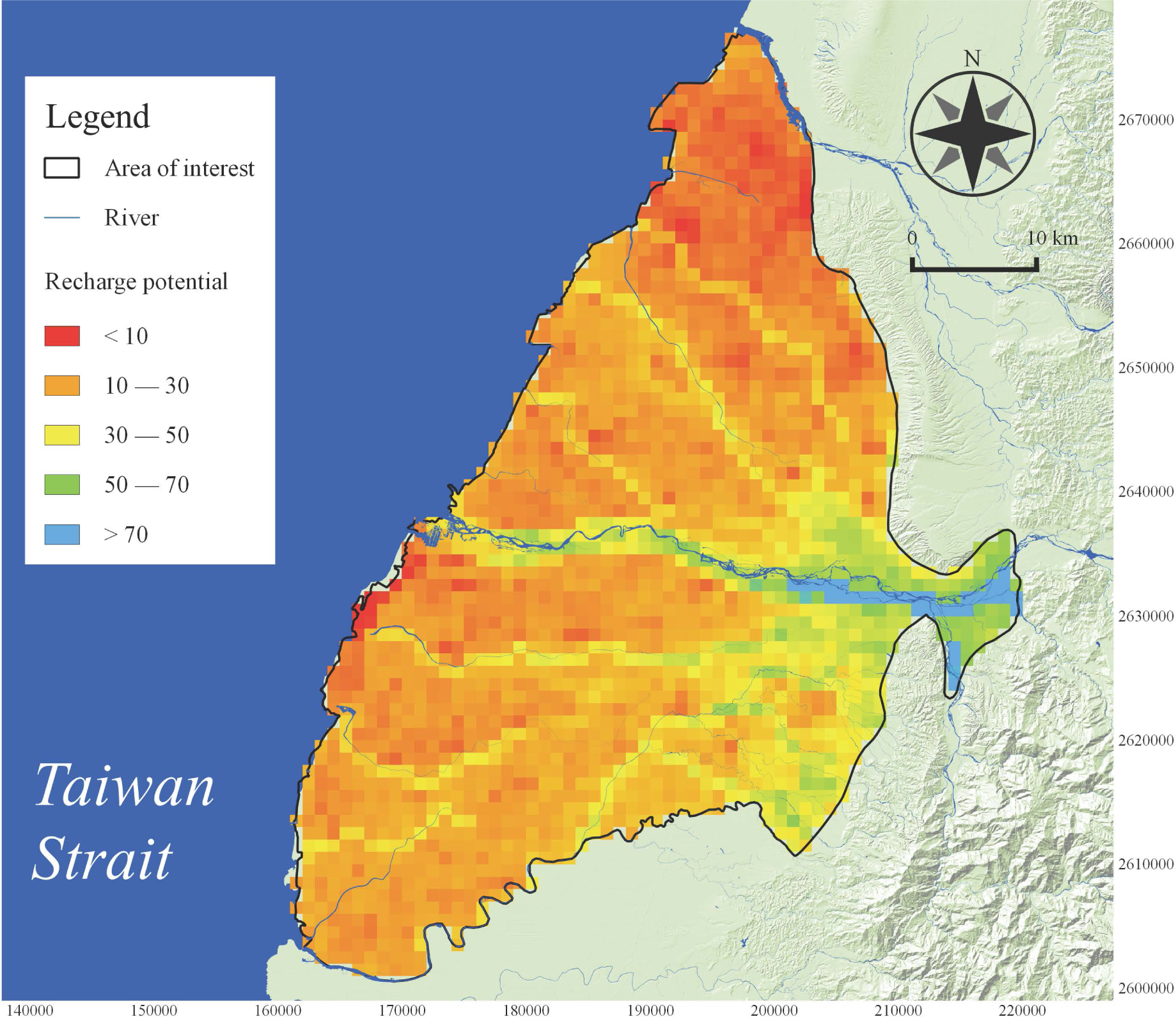
2.1. Study Area

The study area, which consists of Taiwan’s Choushui River alluvial fan, is located on the midwestern part of Taiwan, and it is bounded by the Wu River to the north, the Taiwan Strait to the west, the Beigang River to the south and the Bagua Tableland to the east, as shown in Figure 1.
The primary region of interest is the plain below 100 m in altitude that covers approximately 2150 km2 [16]. This area descends from the east to the west. Five rivers flow through the entire study area and eventually reach the Taiwan Strait. From north to south, they are as follows: the Wu, Old Chuoshui, Chuoshui, New Huwei and Beigang rivers. The primary river of this area is the Chuoshui River.
The Choushui River alluvial fan is located near the Tropic of Cancer, and it has a subtropical climate. The annual rainfall in this area is high, but it is not evenly distributed in time and space. The wet season occurs during April to August, while the dry season occurs during September to the following March. The wet season contributes 79% of the annual rainfall to the study area, while the dry season only contributes 21%. Thus, the rainfall difference between the wet and dry season is significant. The average annual rainfall declines as one moves from the eastern mountains to the coastline areas. Specially, the average annual rainfall in the east mountain area is 2000 mm, and it declines to 1300 to 1600 mm in the alluvial fan areas and 1000 mm in coastline areas.
The Central Geology Survey (CGS) indicated that the hydrogeological structure of the study area can be divided into several strata. Based on the depth from the land surface, these strata are as follows: Aquifer 1, Aquitard 1, Aquifer 2, Aquitard 2 and Aquifer 3. The average thicknesses of Aquifer 1, Aquifer 2 and Aquifer 3 are 42 m, 95 m and 86 m, respectively. The thickness of gravel and sand strata in fan-top areas can reach up to more than 130 m. The aquitards are absent in fan-top areas.
Groundwater is an important water supply in the Choushui River alluvial fan, because the water supplied by the small-scale reservoirs cannot satisfy the water demand of the study area. Chang et al. [17] indicated that the average annual pumpage rates of Aquifer 1, Aquifer 2 and Aquifer 3 are 0.708, 0.32 and 0.23 billion tons per year. The average annual recharge and inflow influenced by seawater are 1.828 and 0.017 billion tons, respectively. The amount of water discharging into a river or through its boundary into another basin is 0.607 billion tons. Thus, the groundwater system almost attains a mass balance situation. However, the demand for groundwater is increasing quickly because of increases in the population size and increases in agricultural and industrial activities. The overuse of groundwater can result in subsidence and seawater intrusion.
To avoid problems associated with groundwater overuse, conservation practices are urgently need; thus, delineation of high recharge areas represents a crucial issue. Accordingly, a systematical methodology was developed to estimate the high recharge areas for the study area. It is hoped that the estimated results will be valuable references for the Taiwanese government to consider when implementing the Land Use Management Act.

2.2. Data

The data used in this study include land use, surface soil, rainfall, river and groundwater well data, which were collected from the Taiwanese government (Table 1).
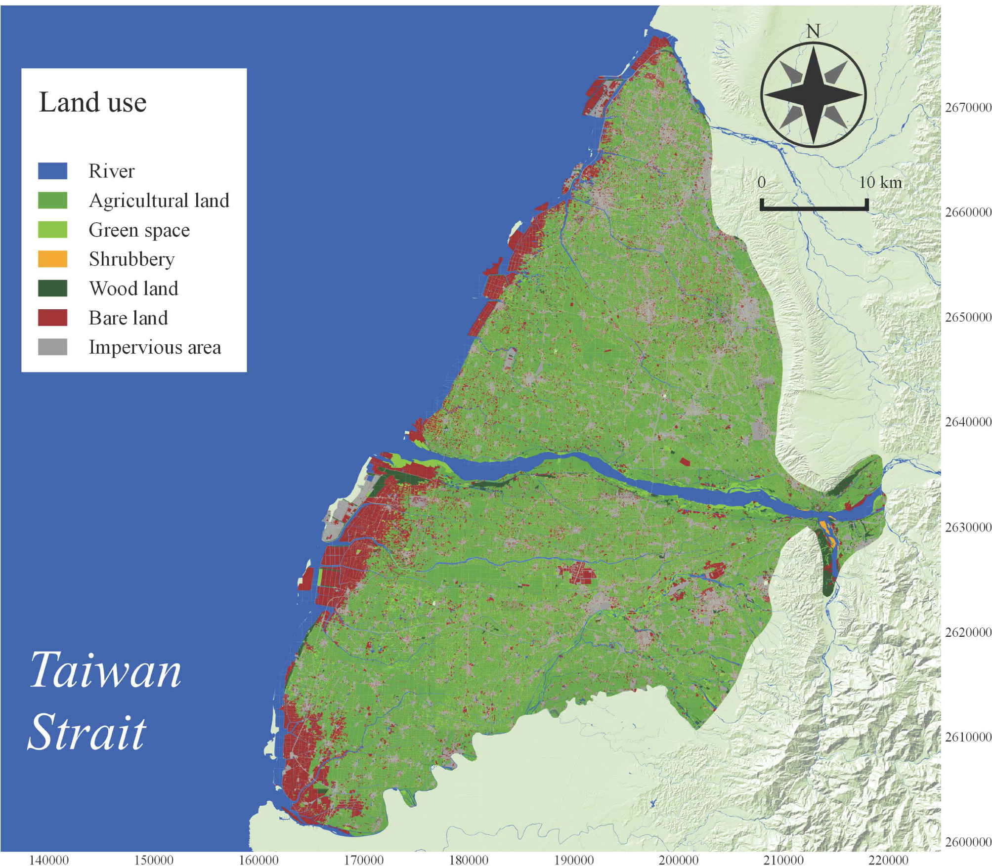
The collected land use and surface soil data are polygon-type data, and these datasets were collected from the CGS and National Land Surveying and Mapping Center, respectively. 
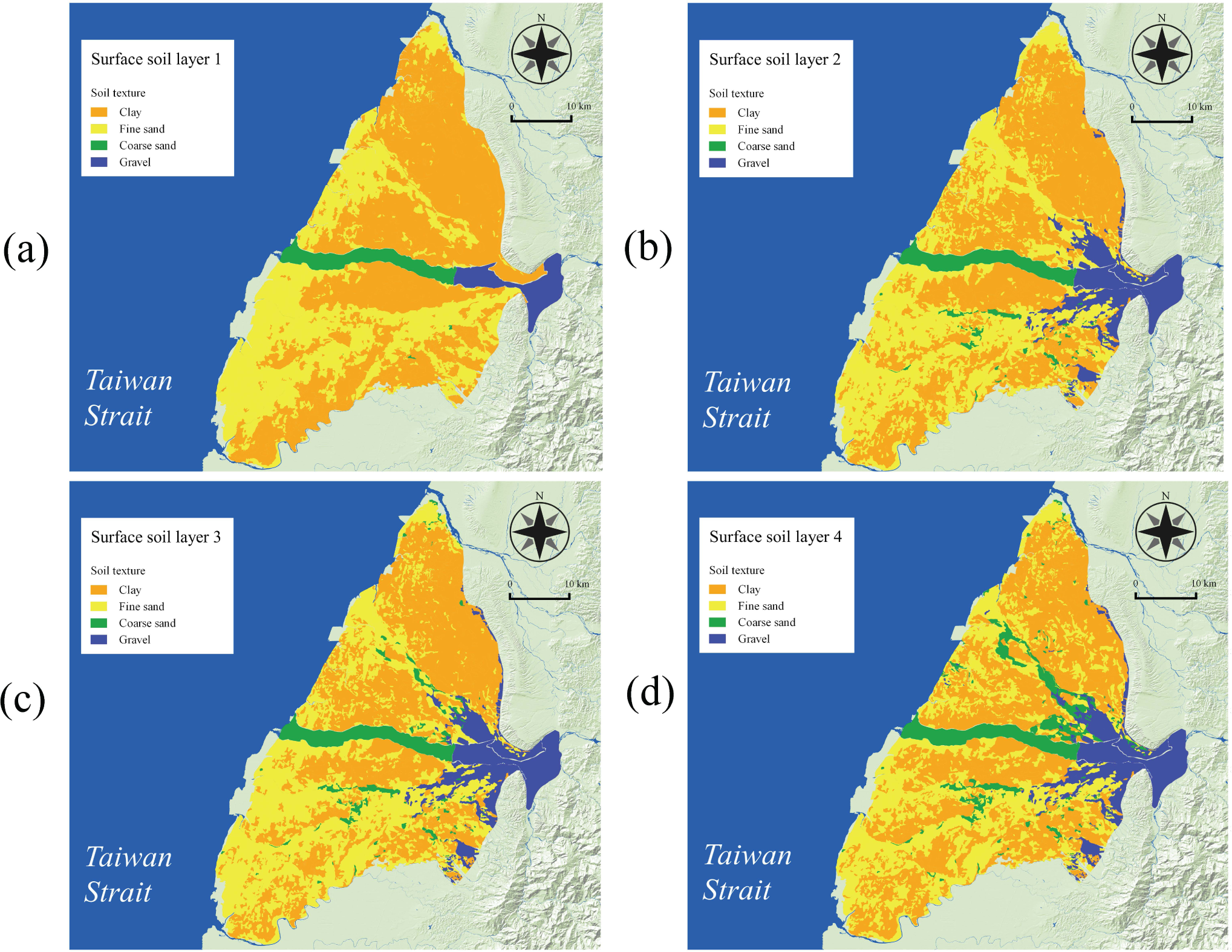
Figure 2 shows the seven attributes of land use, including river, agricultural land, green space, shrubbery, wood land, barren land and impervious land. The CGS also produced surface soil distribution maps with four layers according to the depth from land surface. The depths of the four layers are 0–30, 30–60, 60–90 and 90–150 cm. Each layer has four sediment attributes, including gravel, coarse sand, fine sand and clay, as shown in Figure 3.
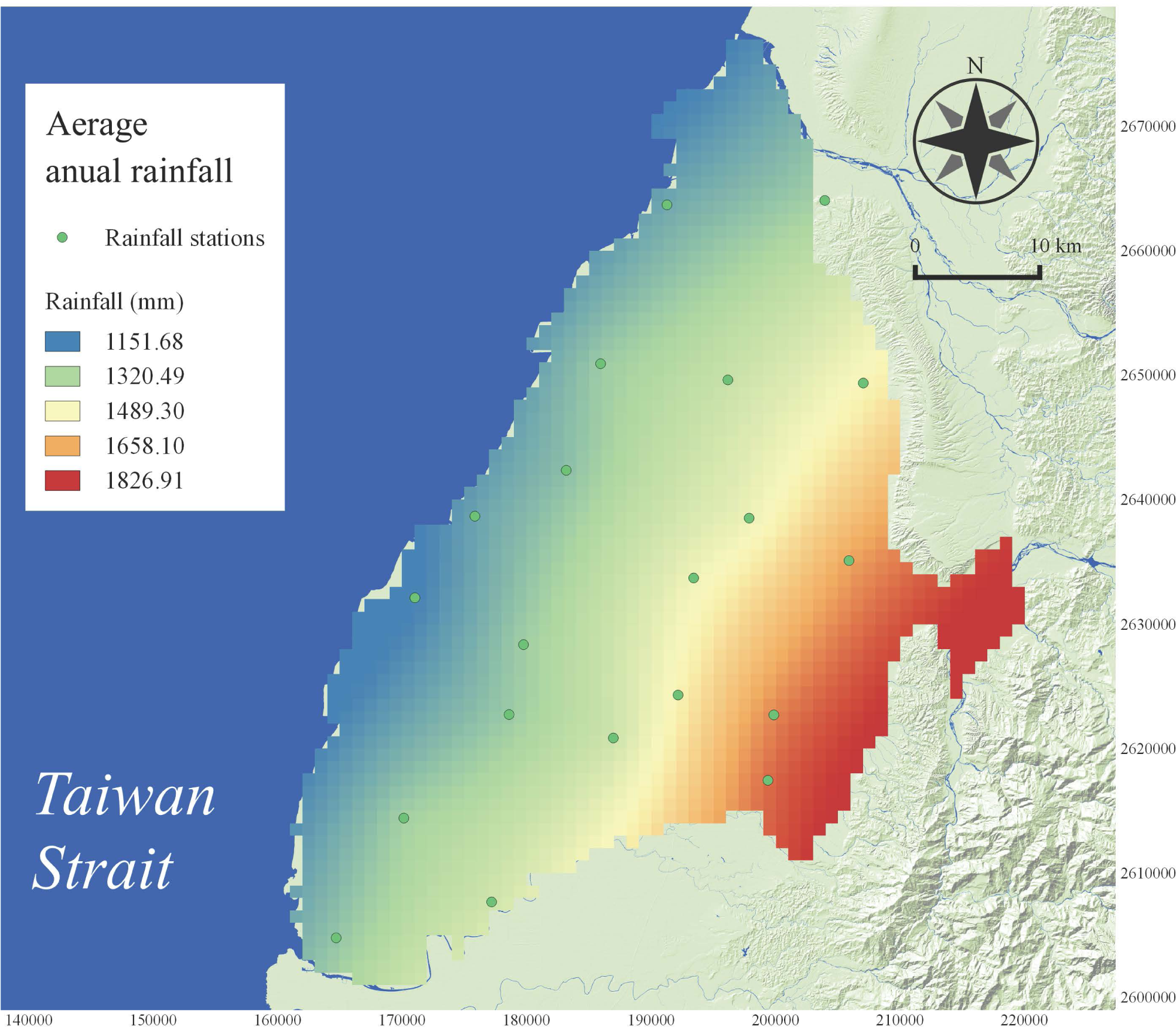
The daily rainfall data from 1998 to 2012 were collected from the Central Weather Bureau (CWB). The selected 20 rainfall stations are located in the Choushui River alluvial fan and in the neighboring mountain areas, as shown in Figure 4.
The collected river data are polyline-type data, and the data were collected from the Water Resources Agency (WRA). The groundwater well data were also collected from the WRA. Because the heads observed in unconfined aquifers were highly correlated with rainfall/stream observations [14,15], the wells located in unconfined aquifers with head observations from 1998 to 2012 were selected to develop the ASV indexes. The locations of the selected wells and the distributions of rivers are shown in Figure 5, respectively.

2.3. Recharge Potential Analysis

The first step of the RPA is to define its contributing factors that influence the groundwater recharge of the study area. Four contributing factors, including land use (CF1), surface soil types (CF2), average annual rainfall (CF3) and drainage density (CF4), were selected, and the reasons for selecting these four factors are described in Section 2.3.1. The descriptions of the four factors are listed in Table 2.
The original GIS maps for the contributing factors were developed by collecting available data within the study area. Each GIS map was converted into a 1 km × 1 km grid map. Point data were interpolated to all the grids using the ordinary kriging method.
Next, the weights and mapping scores of each attribute for the four factors need to be defined according to their contribution to the groundwater recharge. The initial weights and mapping scores were assigned in this study, and these values are shown in Table 3. The initial weights of the four factors were all assigned as 0.25, because the four factors were initially assumed to be of equal importance to the groundwater recharge. The weights of the four factors and the mapping scores of each attribute for CF1 and CF2 were then adjusted through parameter identification, as shown in Section 2.5.
After the factor weights and the mapping scores of each factor’s attributes were identified, the original attributes of the four factors could be converted into scores. Then, the GRP was obtained by computing the weighted sum of the scores from all of the contributing factors. The estimated GRP was graded into five levels, and the data are displayed as a GIS map in the results.

2.3.1. Establishment of Contributing Factors

Four contribution factors were selected by referencing previous studies [1,39,11,12] and considering the environmental conditions of the study area. The reasons for selecting these four factors are described as follows.
  • Land use:
    Land use is important for groundwater recharge. Artificial structures built with concrete will prevent recharge. Shaban et al. [8] have shown that vegetation is good for recharge, because vegetation increases infiltration by loosening soil and catching surface run-off. In addition, Bartens et al. [18] have shown that tree roots can increase infiltration by loosening the compacted soils. Thompson et al. [19] have demonstrated that coarse root mass is correlated with the infiltration capacity in a humid area. Therefore, vegetation with coarse roots should facilitate groundwater recharge in the study area. However, Zhang and Schilling [20] showed that a high density of vegetation can increase the rate of evapotranspiration and decrease infiltration. In the initial scores, this study relied on the work of Zhang and Schilling [20] and assumed that vegetation is poor for groundwater recharge, thereby the polygon with high density vegetation in the land use map was translated into a low score.
  • Surface soil type:
    Soil particle sizes can have a significant influence on the permeability and infiltration capacity. Thompson et al. [19] found that the soil texture was the major factor influencing the infiltration capacity in wet areas. Therefore, surface soil type was considered as a contributing factor. Surface soil type was defined based on the soil particle size and classified into the four following types: gravel, coarse sand, fine sand and clay. The initial attribute scores of CF2 were assigned based on the soil particle size.
  • Average annual rainfall:
    Rainfall in Taiwan varies significantly during the year. Taiwan is located at the confluence of the Eurasian Plate and the Pacific Ocean, where there are frequent occurrences of monsoons, typhoons and Kuroshio currents. This study considered average annual rainfall as a contributing factor to groundwater recharge because the infiltration of natural rainfall is the major source of groundwater recharge in the region. Average annual rainfall from 1998 to 2012 was calculated from the 20 selected rainfall stations maintained by the CWB.
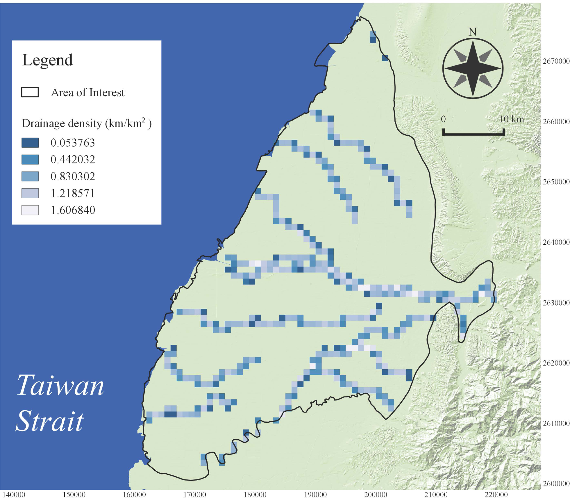
  • Drainage density:
    Drainage density is defined by Hortorn [21] as the total river length per unit area. Dingman [22] noted that drainage density obviously influences the infiltration capacity and soil resistance to erosion. In addition, Kheir et al. [23] and Shaban et al. [8] indicated that drainage is an important factor associated with groundwater recharge. As a result, drainage density was considered as a contributing factor, and it was calculated by using the polyline-type data of the rivers collected from the WRA.

2.3.2. Using GIS to Develop Grade Maps for Each Contributing Factor

Maps of CF1 and CF2 were defined as area attributes using polygons, which means that different polygons can have different attributes. The attribute of each polygon was converted into a score based on Table 3 and Equation (1):
I f S i m = S ¯ i k , then A i m = A ¯ i k for k = 1 , , N and i = 1 , 2
where S is a score between 0 and 100; i is the number of contributing factors; m is the number of polygons; k is the attribute number of each factor; S i m is the factor i score of polygon m; S ¯ i k is the factor i score of attribute k; A is the attribute of a factor; A i m is the factor i attribute of polygon m; and A ¯ i k is the factor i attribute of k.
The GIS maps of CF1 and CF2 were discretized by using a 1 km × 1 km grid, and each grid covers several polygons. After obtaining the score for each polygon, Equation (2) was used to calculate the total score of each grid, and the score maps of CF1 and CF2 were developed.
S i , j = A r e a i m × S i m A r e a i m , m C e l l j
where j is the cell number; Area is the area of a polygon; Si,j is the factor i score of cell j; A r e a i m is the factor i area of polygon m; and Cell is the grid-square of the grid map.
The attributes of CF3 and CF4 are continuous data. The original attributes, such as the average annual rainfall or drainage density, were linearly normalized between 0 and 100. For example, the attributes of CF3 can be normalized by the maximum and minimum average annual precipitation. The equation used to normalize the data is shown in Equation (3):
S i m = F i , j F i m i n F i m a x F i m i n × 100 , for i = 3 , 4
where Fi,j is the factor i attribute of cell j; F i m i n is the minimum attribute of factor i; and F i m a x is the maximum attribute of factor i.

2.3.3. Estimation of Groundwater Recharge Potential

The GRP was calculated as follows:
G R P j = i = 1 4 ω i × S i , j
where GRPj is a weighted sum of all of the factor values and represents the groundwater recharge potential for grid element j; ωi represents the weight associated with factor i.
After estimating GRP for all grid elements, GRP was converted into the following five levels: very poor, poor, moderate, good and excellent. The score ranges of these five levels were 0 to 10 scores, 10 to 30 scores, 30 to 50 scores, 50 to 70 scores and 70+ scores. The mappings between the score ranges and average annual recharge rate per unit area (AARRPA) estimated by Chang et al. [17] are described in Section 3.3. The spatial distribution of GRP is shown by using the five levels, and the results are displayed as a GIS map in the results.

2.4. Development of ASV Indexes

An ASV index represents the average storage variation of a local aquifer, and it was developed by using Equation (5). The observed head changes of each well can be obtained by calculating the standard deviation of its corresponding head observations. Because the heads observed in unconfined aquifers are highly correlated with rainfall, the head observations from the 15 wells located in the unconfined aquifer were selected to calculate the head changes. The aquifer storage capability of each selected well is represented by Sy.
A S V i = σ i × ( S y ) i
where Sy denotes the specific yield and σ denotes the standard deviation of observed heads where i denotes the well number.

2.5. Using the Simulated Annealing Algorithm to Calibrate RPA Parameters Based on ASV Indexes

The initial RPA parameter values were adjusted according to parameter identification theory. The identification of RPA parameters was formulated as a minimization problem. Simulated annealing (SA) was used to minimize the object function (the difference between the GRP values and the ASV indexes), because the relationship between ASV indexes and GRP may be nonlinear. The correlations between the ASV indexes and estimated GRP values were used to evaluate the correctness of RPA parameters. After parameter calibration, the correlations between the GRP values and ASV indexes are excepted to be improved.
This study develops 15 ASV indexes for the RPA parameter calibration. The RPA parameters include CF1’s seven attribute scores, CF2’s three attribute scores and the weights of the four contributing factors. Although ASV indexes are suitable to be used as the surrogate variable of GRP, in practice, the number of ASV indexes are limited because of the high expense of well-drilling. Therefore, high density head samples are difficult to obtain and unrealistic.
To properly use limited ASV indexes, an ASV index representing the recharge ability of a selected grid was assumed. If a grid has a well, the ASV index calculated from this well’s information was assumed to represent the recharge ability of the grid area. Thus, comparisons of how close the values are between the ASV indexes and the selected grid’s GRP value are possible because both represent the grid area’s recharge ability. In addition, the selected grids must cover all of the four factors’ original attributes, such as the polygons for CF1’s seven attributes and CF2’s three attributes. Therefore, the selected grids’ GRP values will vary with the RPA parameter adjustments, and all of these RPA parameters can be calibrated.
To compare the estimated GRP values with the ASV indexes, these two datasets were normalized between 0 and 100. The goal of the objective function Equation (6) is to minimize the difference between the ASV indexes and the GRP values. The purposes of the constraint functions Equations (7) to (10) are to constrain the range of the 15 parameters.
The mathematical formulations of this minimization problem are shown in Equations (6) to (10):
f = m i n ( l = 1 l = 15 ( A S V l G R P l ) 2 )
s.t.
0 S ¯ 1 k 1 100 , for k 1 = 1 , 2 , , 7
0 S ¯ 2 k 2 100 , for k 2 = 1 , 2 , 3 , 4
0 w i 1 , for i = 1 , 2 , 3 , 4
i = 1 i = 4 w i = 1
where l denotes the 15 grids with the observation wells in the study area; k1 denotes the attribute number of CF1; k2 denotes the attribute number of CF2; S ¯ 1 k 1 denotes the k1-th attribute score of CF1; S ¯ 2 k 2 denotes the k2-th attribute score of CF2; and wi denotes the weighting of contributing factor i.
The SA algorithm was applied to solve this minimization problem; SA is a search-based optimization method that was developed by Kirkpatrick et al. [24]. A material can be transferred into another matter with different crystalline structures by heating and cooling process. The crystalline structure varies with different cooling rates. If each crystalline structure represents a possible solution in the solution spaces for a problem, the crystalline structure with the minimum energy state is the optimal solution [25].
Simulated annealing can search for the global optimal solution for a problem by considering bad trials. The search algorithm for SA was developed by considering a random number with a normal distribution and a Metropolis algorithm [26] to determine the acceptance of the new solution. In the Metropolis algorithm, the acceptance probability is formulated as a Boltzmann probability density function:
P = { 1 , i f Δ E 0 e Δ E / K T , i f Δ E > 0
where P denotes the probability of the Metropolis mechanism; ΔE denotes the change of energy between the old solution and new solution; T denotes the temperature; and K denotes the Boltzmann constant. If the objective function is improved (system energy is reduced), the adjacent solution will be accepted; if not, the adjacent solution will still have the opportunity to be accepted depending on the acceptance probability and the energy change between the two iterations [26].
The input parameters of SA are initial temperature, terminal temperature, cooling rate and maximum iterations of each temperature. These parameters are associated with the “temperature schedule” strategy, which affects the searching paths and the optimization results. These parameter values are not unique and need to be adjusted based on the problem domain. In this study, the parameter values were determined by a “trial-and-error” process. The initial temperature was set to 1000; the terminal temperature was set to 1; the cooling rate was set to 0.97; and the maximum iterations of each temperature was set to 200. The bounds of the decision variables are defined by the constraints, as shown in Equations (7) to (10).

3. Results and Discussion

3.1. Original GIS Maps for the Four Contributing Factors

In this study, data associated with land use and surface soil type were explicitly defined in the GIS map and are shown by polygons. Other contributing factors required the kriging method to interpret field survey data for every node in the 1 km by 1 km GIS map grid. The original attributes associated with each contributing factor are described as follows:
  • Land use:
    The land use map shows that agricultural lands (yellow green color) are distributed uniformly in the study area (Figure 2). The impervious areas shown with the gray color are located in cities and industrial areas; these areas are covered with concrete. The barren lands shown with the red color are mainly located along the coastline. The green spaces shown with the light green color are mainly located in the areas close to the rivers. The cell-based score map of land use was calculated from its polygon-based attribute map by using Equation (2).
  • Surface soil:
    The soil data from the CGS consists of four soil layers. The depths of these soil layers range from 0 to 30 cm, 30 to 60 cm, 60 to 90 cm and 90 to 120 cm. Figure 3 shows CF2’s original maps and illustrates that most gravel is located in the fan-top areas of the Choushui River. The colors of clay and fine sand are orange and yellow, respectively. The areas on the north side and south side of the Choushui River are mostly covered by clay and fine sand, respectively. A few areas close to the rivers covered by coarse sand are shown with the green color. The cell-based score map of each soil layer was calculated by using Equation (2). The cell-based score map of CF2 was calculated by averaging the cell-based score maps of the four soil layers.
  • Average annual rainfall:
    The ordinary kriging method was used to interpolate the average annual rainfall from the 20 selected rainfall stations to the center of each grid element. Figure 4 shows that the rainfall decreases from the mountains to the seashore. The cell-based score map of CF3 was calculated from its attribute map by using Equation (3).
  • Drainage density:
    Drainage density was calculated by using Equation (12). The unit area was set corresponding to the map grid with an area of 1 km2, and therefore, the drainage density equals the total river length within a grid. The distribution of drainage density is shown in Figure 6. The cell-based score map of CF4 was calculated from its attribute map by using Equation (3).
    D = L / A r e a u n i t
    where D denotes the drainage density; Areaunit denotes the unit area in km2; and L denotes the river length in km inside the unit area.

3.2. Results for the ASV Index

Table 4 shows the estimated results for the ASV indexes. The collected head observations from 1998 to 2012 were used to compute the standard deviation of the heads (STDH) of each selected well, and the range of the STDH values was between 0.38 to 2.66 m. The ASV index was calculated by using Equation (5), and the values ranging from 0.007 to 0.529 were normalized to between 1.34 % and 100%. To serve as a calibration reference for the RPA, the values of ASV were multiplied by 100. The maximum and minimum values of ASV were 100 and 1.34, respectively.

3.3. Calibration Results for the RPA

The calibration procedure adjusts the distribution of GRP values to be close to the distribution of ASV values in the 15 selected wells. Table 5 shows the ASV and GRP values before and after parameter calibration in the 15 selected wells. Before parameter calibration, the value distributions of GRP and ASV datasets were different and had a correlation coefficient of 0.67. After parameter calibration, the correlation coefficient increased to 0.85. Thus, the correlation between GRP and ASV was significantly improved.
Table 6 shows that the weights of the contributing factors before and after parameter identification are significantly different. The calibrated weight of CF2, surface soil, accounts for the highest proportion of the weighted sum of the four factors. This result indicates that CF2 mostly influences the long-term groundwater recharge resulting from the surface soil of the upstream areas of the Choushui River that consist of gravel with high permeability, while that of the middle and downstream areas were composed of fine grains with poor permeability. Thus, the groundwater recharge is under the constraint of the spatial distribution of coarse and fine grains. Thompson et al. [19] also founded that soil texture significantly influences the infiltration in a humid area. Therefore, the calibrated weight of CF2 is reasonable.
The estimated weight of CF1, land use, was the second highest value among the four factors. The coarse vegetation roots and how the land is being used affect the groundwater recharge. Thompson et al. [19] indicated that coarse root mass can influence the infiltration capacity for a wet area, because the coarse roots can increase the infiltration by loosening the rocks and compacted soils. Impervious areas, which are largely covered by concrete, prevent the surface water from infiltrating into an aquifer and are associated with extremely low infiltration capacity. Thus, land use type affects how the surface water infiltrates into the soil layers. Because more than 60% of the land use type of the study area was paddy fields and less than 15% was impervious areas, most surface water can reach the soil layers, but the soil texture determines the amount of surface water reaching the aquifers. Therefore, CF1 had less of an influence on the groundwater recharge than CF2 in the study area.
Both the estimated weights of CF3 (average annual rainfall) and CF4 (drainage density) were low. These results show that CF3 and CF4 only slightly influence the groundwater recharge, because wet areas usually have sufficient recharge sources. Therefore, the land use and soil texture are the major factors that dominate the recharge of the study area.
The calibration results show that vegetation roots are correlated with groundwater recharge, which confirm the results of the previous studies [8,18,19]. Table 7 shows the attribute scores of CF1 (land use) before and after parameter calibration. The calibrated scores of the wood land and shrub land are much higher than those of grass land. This also indicates that the land use types with coarse-root vegetation are good for groundwater recharge. The scores for barren areas are low because no coarse-root vegetation was observed in these areas.
The attribute score of agricultural land was adjusted from 90.00 to 59.95, which is not as high as expected given the initial scores. The attribute score of agricultural land was supposed to be high, because the land surfaces of the agriculture lands are covered by water during the cultivation period, which results in continuous infiltration. However, the hardpan layer located 20–40 cm under the surface of the paddy fields reduces soil leakage and makes it difficult for water to infiltrate into the aquifer [2730]. Therefore, the contribution of agriculture land to the groundwater recharge is moderate, and the estimated attribute score is reasonable.
Table 8 shows that the estimated attribute values of CF2, surface soil. The score distribution shows that gravel is the best material for groundwater recharge. Additionally, coarse sand and fine sand are relatively good materials for groundwater recharge compared to clay, which was found to be the worst. The calibrated scores of coarse sand and fine sand are less than the initial scores because their formations may mix with clayey matter.
Figures 7 and 8 show the recharge potential maps before and after the RPA parameter calibration. Figure 7 was developed by using the initial guesses of RPA parameters, while Figure 8 was developed by using the calibrated RPA parameters. The GRP distributions of these two maps are different. In the recharge potential maps, the colors indicate the levels of GRP: blue color denotes excellent, green color denotes high, yellow color denotes moderate, orange denotes poor and red denotes very poor. Figure 8 shows that the fan-tops of the Choushui River alluvial fan are in high and excellent GRP levels, and the mid-fan and fan-tail areas are in poor and very poor GRP levels. The areas with moderate GRP levels are located along the Choushui River. The GRP map was further compared to the map of AARRPA estimated by Chang et al. [17], and the mappings between the GRP levels and AARRPA were developed and shown as follows:
  • Excellent GRP level = 1.86 m/year.
  • High GRP level = 1.14 m/year.
  • Moderate GRP level = 0.98 m/year.
  • Poor GRP level = 0.71 m/year.
  • Very poor GRP level = 0.23 m/year.
Table 9 shows the area statistics of the five GRP levels before and after parameter calibration. After the parameter calibration process, the areas with excellent GRP level were expanded by 226.60%, the high GRP level areas were reduced by 76.23%, the moderate GRP level areas were reduced by 88.06%, the poor GRP level areas were expanded by 59.08%, and the very poor GRP level areas were expanded by 5910.04%.
In other words, using the initial RPA parameter values to estimate the recharge potential map may overestimate the moderate and high GRP level areas and underestimate the excellent, poor and very poor GRP level areas.
This study defines areas with high and excellent GRP levels as high recharge areas, and these areas were located in the upstream areas of the Choushui River. The total amount of high recharge areas was approximately 170.58 km2, which amounts to 7.92% of the study area.

4. Conclusions

This study developed a systematic approach to objectively define the RPA parameter values by using a parameter estimation approach based on 15 ASV indexes. The results show that the GRP values estimated by the calibrated RPA parameters were highly correlated with the ASV indexes. The calibrated RPA parameters represent the field infiltration characteristic of the study area well, and therefore, the estimated GRP can be used to delineate the high recharge areas with high accuracy. In other words, estimating the GRP distribution by using the calibrated RPA parameter values is more accurate and objective than that estimated by using the suppositional RPA parameter values. Therefore, defining the RPA parameter values with ASV indexes is crucial for better accuracy. The estimated RPA parameters also allowed us to realize the contribution of the factors to the groundwater recharge and are valuable for understanding the mechanisms of groundwater recharge for the study area. The developed approach can be applied to other study areas by replacing suitable contributing factors based on an areas’ climate, hydrology, geology and human activities. On the basis of the developed method, the field infiltration characteristics of such study areas can be identified through the estimated GRP spatial distribution, and the study results will likely be valuable references for regional groundwater resource management efforts.

Acknowledgments

The authors would like to thank the National Science Council and Central Geological Survey, Taiwan, for financially supporting this research under Contract Nos. NSC101-2625-M-009-003 and MOEA101-5926901000-03-01, respectively.

Author Contributions

Jui-Pin Tsai wrote this paper, developed the numerical model for recharge potential analysis (RPA) and integrated the optimization model with the RPA model; Yu-Wen Chen developed the optimization model based on simulated annealing algorithm; Liang-Cheng Chang designed this research; Yi-Ming Kuo assisted the development of RPA model; Yu-Hsuan Tu analyzed the data and developed the GIS maps; Chen-Che Pan analyzed the data and assisted the development of optimization model. All authors have read and approved the final manuscript.

Conflicts of Interest

The authors declare no conflict of interest.

References

  1. Bromley, J.; Edmunds, W.; Fellman, E.; Brouwer, J.; Gaze, S.; Sudlow, J.; Taupin, J. Estimation of rainfall inputs and direct recharge to the deep unsaturated zone of southern Niger using the chloride profile method. J. Hydrol. 1997, 188, 139–154. [Google Scholar]
  2. Brito, M.; Costa, C.; Almeida, J.; Vendas, D.; Verdial, P. Characterization of maximum infiltration areas using GIS tools. Eng. Geol. 2006, 85, 14–18. [Google Scholar]
  3. Chenini, I.; Mammou, A.B.; El May, M. Groundwater recharge zone mapping using GIS-based multi-criteria analysis: A case study in Central Tunisia (Maknassy Basin). Water Resour. Manag. 2010, 24, 921–939. [Google Scholar]
  4. Jasrotia, A.; Kumar, R.; Saraf, A. Delineation of groundwater recharge sites using integrated remote sensing and GIS in Jammu district, India. Int. J. Remote Sens. 2007, 28, 5019–5036. [Google Scholar]
  5. Mondal, N.; Singh, V. A new approach to delineate the groundwater recharge zone in hard rock terrain. Curr. Sci. 2004, 87, 658–662. [Google Scholar]
  6. Mukherjee, P.; Singh, C.; Mukherjee, S. Delineation of Groundwater potential zones in arid region of India—A remote sensing and GIS approach. Water Resour. Manag. 2012, 26, 2643–2672. [Google Scholar]
  7. Salama, R.B.; Tapley, I.; Ishii, T.; Hawkes, G. Identification of areas of recharge and discharge using Landsat-TM satellite imagery and aerial photography mapping techniques. J. Hydrol. 1994, 162, 119–141. [Google Scholar]
  8. Shaban, A.; Khawlie, M.; Abdallah, C. Use of remote sensing and GIS to determine recharge potential zones: The case of Occidental Lebanon. Hydrogeol. J. 2006, 14, 433–443. [Google Scholar]
  9. Yeh, H.F.; Lee, C.H.; Hsu, K.C.; Chang, P.H. GIS for the assessment of the groundwater recharge potential zone. Environ. Geol. 2009, 58, 185–195. [Google Scholar]
  10. Arnold, T.L.; Friedel, M.J. Effects of Land Use on Recharge Potential of Surficial and Shallow Bedrock Aquifers in the Upper Illinois River Basin; Water-Resources Investigations Report 2000–4027; U.S. Department of the Interior, U.S. Geological Survey: Urbana, IL, USA, 2000; U.S. Geological Survey, Information Services: Denver, CO, USA, 2000.
  11. Mukherjee, S. Targeting saline aquifer by remote sensing and geophysical methods in a part of Hamirpur-Kanpur, India. Hydrogeol. J. 1996, 19, 53–64. [Google Scholar]
  12. Soares, P.; Pereira, S.; Simoes, S.; de Paula Bernardes, G.; Barbosa, S.; Trannin, I. The definition of potential infiltration areas in Guaratinguetá watershed, Paraíba do Sul Basin, Southeastern Brazil: An integrated approach using physical and land-use elements. Environ. Earth Sci. 2012, 67, 1685–1694. [Google Scholar]
  13. Braun, G.M.; Levine, N.S.; Roberts, S.J.; Samel, A.N. A geographic information systems methodology for the identification of groundwater recharge areas in Waukesha County, Wisconsin. Environ. Eng. Geosci. 2003, 9, 267–278. [Google Scholar]
  14. Yu, H.L.; Chu, H.J. Understanding space-time patterns of groundwater system by empirical orthogonal functions: A case study in the Choshui River alluvial fan, Taiwan. J. Hydrol. 2010, 381, 239–247. [Google Scholar]
  15. Yu, H.L.; Chu, H.J. Recharge signal identification based on groundwater level observations. Environ. Monit. Assess. 2012, 184, 5971–5982. [Google Scholar]
  16. CGS. Groundwater Observation Well Network Phase I: The Application of Geophysical Exploration and Stratum Study; Technical Report; Central Geological Survey, MOEA: Taipei City, Taiwan, 1995. [Google Scholar]
  17. Chang, L.C.; Chen, W.F.; Chang, P.Y.; Chen, Y.W. Hydrogeology Investigation and Groundwater Resource Assessment for Taiwan: Groundwater Recharge Estimation and Model Simulation–Choushui River Alluvial Fan; Technical Report; Central Geological Survey, MOEA: Taipei City, Taiwan, 2012. [Google Scholar]
  18. Bartens, J.; Day, S.D.; Harris, J.R.; Dove, J.E.; Wynn, T.M. Can urban tree roots improve infiltration through compacted subsoils for stormwater management? J. Environ. Q. 2008, 37, 2048–2057. [Google Scholar]
  19. Thompson, S.E.; Harman, C.J.; Heine, P.; Katul, G.G. Vegetation-infiltration relationships across climatic and soil type gradients. J. Geophys. Res. Biogeosci. (2005–2012) 2010, 115. [Google Scholar] [CrossRef]
  20. Zhang, Y.K.; Schilling, K. Effects of land cover on water table, soil moisture, evapotranspiration, and groundwater recharge: A field observation and analysis. J. Hydrol. 2006, 319, 328–338. [Google Scholar]
  21. Horton, R.E. Drainage-basin characteristic. Eos Trans. AGU 1932, 13, 350–361. [Google Scholar]
  22. Dingman, S.L. Drainage density and streamflow: A closer look. Water Resour. Res. 1978, 14, 1183–1187. [Google Scholar]
  23. Kheir, R.B.; Shaban, A.; Girard, M.C.; Khawlie, M.; Abdallah, C. Caractérisation morpho-pédologique des zones karstiques du Liban Sensibilité des sols à l‘érosion hydrique. Science et Changements Planétaires/Sécheresse 2003, 14, 247–255, In French. [Google Scholar]
  24. Kirkpatrick, S.; Gelatt, C.D.; Vecchi, M.P. Optimization by simmulated annealing. Science 1983, 220, 671–680. [Google Scholar]
  25. Yeh, H.D.; Chang, T.H.; Lin, Y.C. Groundwater contaminant source identification by a hybrid heuristic approach. Water Res. Res. 2007, 43, W09420. [Google Scholar]
  26. Metropolis, N.; Rosenbluth, A.W.; Rosenbluth, M.N.; Teller, A.H.; Teller, E. Equation of state calculations by fast computing machines. J. Chem. Phys. 1953, 21, 1087–1092. [Google Scholar]
  27. Aimrun, W.; Amin, M.; Eltaib, S. Effective porosity of paddy soils as an estimation of its saturated hydraulic conductivity. Geoderma 2004, 121, 197–203. [Google Scholar]
  28. Tournebize, J.; Watanabe, H.; Takagi, K.; Nishimura, T. The development of a coupled model (PCPF-SWMS) to simulate water flow and pollutant transport in Japanese paddy fields. Paddy Water Environ. 2006, 4, 39–51. [Google Scholar]
  29. Vu, S.H.; Ishihara, S.; Watanabe, H. Exposure risk assessment and evaluation of the best management practice for controlling pesticide runoff from paddy fields. Part 1: Paddy watershed monitoring. Pest Manag. Sci. 2006, 62, 1193–1206. [Google Scholar]
  30. Wu, R.S.; Sue, W.R.; Chien, C.B.; Chen, C.H.; Chang, J.S.; Lin, K.M. A simulation model for investigating the effects of rice paddy fields on the runoff system. Math. Comput. Model. 2001, 33, 649–658. [Google Scholar]
Figure 1. Map of the study area over a digital elevation model.
Entropy 17 01558f1
Figure 2. Land use map of the Choushui River alluvial fan.
Entropy 17 01558f2
Figure 3. The distribution maps for four types of surface soil categorized by their depths from the land surface. (a) 0–30 cm; (b) 30–60 cm; (c) 60–90 cm; (d) 90–150 cm.
Entropy 17 01558f3
Figure 4. Average annual rainfall map of the Choushui River alluvial fan.
Entropy 17 01558f4
Figure 5. Positions of the 15 selected wells in the study area.
Entropy 17 01558f5
Figure 6. Drainage density map of the Choushui River alluvial fan.
Entropy 17 01558f6
Figure 7. Groundwater recharge potential (GRP) distribution before the recharge potential analysis (RPA) parameter calibration.
Entropy 17 01558f7
Figure 8. Groundwater recharge potential (GRP) distribution after the recharge potential analysis (RPA) parameter calibration.
Entropy 17 01558f8
Table 1. The name and source of the collected data.
Data NameData SourceData Type
Groundwater well dataWater Resource AgencyRaw data
RainfallCentral Weather BureauRaw data
Land useNational Land Surveying and Mapping CenterShape file (polygon-type data)
Surface soilCentral Geology SurveyShape file (polygon-type data)
DrainageWater Resource AgencyShape file (polyline-type data)
Table 2. The selected four contributing factors for estimating the groundwater recharge potential.
Contributing FactorSymbolDescription
Land useCF1The type of land use and land cover
Surface soil typeCF2The distribution of surface soil type from 0 cm to 150 cm
Average annual rainfallCF3The long-term average annual rainfall
Drainage densityCF4The total river length per unit area
Table 3. The initial weights and attribute scores of the four contributing factors.
Contributing FactorsInitial WeightsAttributesInitial Attribute Scores
CF10.25River100
Agricultural land90
Grass land50
Shrub land30
Wood land20
Barren90
Impervious land0

CF20.25Gravel100
Coarse sand70
Fine sand30
Clay0

CF30.253344 (maximum)100
1895 (minimum)0

CF40.256.27 (maximum)100
0 (minimum)0
Table 4. The estimated results for the average storage variation (ASV) indexes.
Well NameSTDH1(m)SyASV (m)Normalized ASVTranslated ASV
Ershuei2.6580.1990.529100.00%100.00
Wutu2.4350.1520.37069.97%69.97
Hesing0.8880.2250.20037.76%37.76
Sijhou0.8030.2160.17432.80%32.80
Ganyuan1.3180.1200.15829.91%29.91
Bozih1.4290.0380.05410.21%10.21
Wuncuo1.2070.0420.0509.47%9.47
Kanjiao1.1130.0430.0489.13%9.13
Fongrong1.3650.0350.0489.04%9.04
Jioujhuang0.9230.0370.0346.46%6.46
Honglun0.7930.0320.0254.75%4.75
Wunchang0.5290.0380.0203.79%3.79
Jioulong0.9990.0140.0142.64%2.64
Tianwei0.6460.0160.0101.92%1.92
Tianyang0.3770.0190.0071.34%1.34
1STDH denotes the standard deviation of the head observations of each selected well.
Table 5. The groundwater recharge potential (GRP) values in the 15 selected wells before and after parameter calibration.
Well NameASV1 IndexesGRP Values before CalibrationGRP Values after Calibration
Ershuei100.0061.8875.34
Wutu69.9766.7667.97
Hesing37.7628.8611.34
Wunchang37.0828.1512.66
Sijhou32.8029.5811.30
Ganyuan29.9144.8025.77
Tianyang13.1131.7713.08
Bozih10.2126.0711.72
Wuncuo9.4744.7612.58
Kanjiao9.1348.2829.85
Fongrong9.0426.7911.55
Jioujhuang6.4636.7314.28
Honglun4.7536.9217.82
Jioulong2.6430.4810.26
Tianwei1.9232.9414.67
1ASV denotes the average storage variation.
Table 6. The weights of contributing factors before and after parameter calibration.
The Name of WeightsWeights before CalibrationWeights after Calibration
Land use25.00%21.72%
Surface soil25.00%76.58%
Average annual rainfall25.00%0.37%
Drainage density25.00%1.33%
Table 7. The attribute scores of land use before and after parameter calibration.
Attribute NameBefore CalibrationAfter Calibration
River100.0099.79
Agriculture land90.0059.95
Grass land50.000.92
Shrub land30.0070.03
Wood land20.0071.85
Barren90.0028.58
Impervious land0.000.00
Table 8. The attribute scores of surface soil before and after parameter calibration.
Attribute NameBefore CalibrationAfter Calibration
Gravel100.0099.95
Coarse sand70.0040.48
Fine sand30.0015.03
Clay0.000.87
Table 9. The areas of the five groundwater recharge potential (GRP) levels before and after calibration.
GRP LevelsAb1 (km2)Aa2 (km2)Aa−b3 (km2)Aa−b/Ab
Excellent34.20111.7077.50226.60%
High247.7158.88188.8376.23%
Moderate987.14117.82869.3288.06%
Poor876.621394.51517.8959.08%
Very poor7.83470.59462.765910.04%
Total2153.502153.500.00
1Ab denotes the area before calibration;
2Aa denotes the area after calibration;
3Aa−b denotes Aa minus Ab.

