1. Introduction
Fractional-derivative models have been increasingly used in the last two decades to quantify anomalous diffusion in disordered systems [
1,
2]. The entropy theory was also combined with fractional calculus in analyzing fractional dynamics with a power-law memory [
3]. For example, El-Wakil and Zahran [
4] applied the maximum entropy principle to reveal the structure of the probability distribution function of waiting times underlying the fractional Fokker-Planck equation. Machado [
5] analyzed multi-particle systems with fractional order behavior. Ubriaco [
3] applied Fisher’s information theory based on his new definition of fractional entropy [
6] to derive mathematical models for anomalous diffusion. Machado [
7] found a power law evolution of the system energy and the entropy measures in fractional dynamical systems filled with colliding particles. Here, we focus on fractional porous media equations, which may also be related to the entropy solution theory [
8].
Porous media focused on by the hydrologic community are known as complex dynamic systems containing multi-scale heterogeneity, but the application of the fractional engine is limited [
9], due to probably two reasons. First, the second-order advection-dispersion equation (ADE) is believed by the hydrologic community to be valid. Most hydrologic numerical models are grid-based, where each grid is homogeneous. Transport within the grid is assumed to be scale-independent normal diffusion, which can be quantified by the ADE. The available, detailed subsurface heterogeneity can then be embedded in the model using a combination of millions of grids. Therefore, although contaminant transport through heterogeneous porous media from pore to regional scales has been well documented to be non-Fickian (as characterized by heavy tails in tracer breakthrough curves (BTC) [
10,
11]), the second-order ADE model with a certain resolution of velocity remains the routine modeling tool in the field of hydrology. For readers interested in this topic, we refer to the most recent comments and replies on the feasibility of the ADE-based models [
12,
13,
14,
15]. Second, the fractional-derivative models do describe anomalous diffusion more efficiently than the standard ADE [
9], but they also introduce additional parameters (such as the fractional order), whose linkage with medium properties may remain obscure.
Critical questions however remain for hydrologic numerical models that have been used for decades. First, does the transport through typical homogeneous porous media remain as scale-independent normal diffusion? If not, then the classical ADE-based modeling tool is questionable. This leads to the subsequent question: could the fractional-derivative model be the appropriate alternative to the ADE for transport in the deceptively simple homogeneous media? In other words, does the diffusion through homogeneous media exhibit fractional dynamics with a power-law memory in either space or time or both? Finally, for practical applications, what are the main factors affecting the fractional-derivative model parameters? These critical questions motivated this study.
The rest of the paper is organized as follows. In
Section 2, we introduce the systematic laboratory transport experiments focusing on the dynamics of nonreactive tracers moving through sand columns of various lengths. Relatively uniform silica sand was used to fill the columns, forming an ideal porous medium that is much more homogeneous than the natural geological medium. In
Section 3, we quantify the observed dynamics using both the classical ADE and different fractional-derivative models. The questions raised above are then discussed in
Section 4. Finally, conclusions are drawn in
Section 5.
2. Laboratory Experiments of Tracer Transport in Sand Columns
2.1. Experimental Setup
We packed glass tubes (with an inner diameter of 25 mm) using silica sand with a relatively uniform size. The corresponding median grain size packed in each tube was 0.73 mm (
i.e., coarse sand), 0.35 mm (medium sand), and 0.21 mm (fine sand), respectively. The silica sand was soaked in nitric acid for 24 h, and then washed with tap water and deionized (DI) water. After drying in an oven, the sand is ready for packing. Finally, the glass columns were packed using the wet sand loading method (which can minimize the air bubbles [
16]), and the resultant porosity was measured (
Table 1). To test the scale effect, we built sand columns with three different lengths of 10 cm, 20 cm and 40 cm.
Table 1.
Parameters used in the models.
R denotes the median grain size.
v and
are the velocity and dispersion coefficient used in the advection-dispersion (ADE) model in Equation (
1), respectively.
γ is the order of the time fractional derivative in the fractional-derivative models in Equations (
3) and (
5).
λ is the tempering parameter,
r is the scale factor and
is the dispersion coefficient in the tempered-stable, fractional advection-dispersion (TS-FADE) model in Equation (
5).
Table 1.
Parameters used in the models. R denotes the median grain size. v and are the velocity and dispersion coefficient used in the advection-dispersion (ADE) model in Equation (1), respectively. γ is the order of the time fractional derivative in the fractional-derivative models in Equations (3) and (5). λ is the tempering parameter, r is the scale factor and is the dispersion coefficient in the tempered-stable, fractional advection-dispersion (TS-FADE) model in Equation (5).
| Column length | R | Porosity | v | | γ | λ | r | |
|---|
| cm | mm | [-] | cm/min | cm/min | [-] | min | min | cm/min |
|---|
| 10 | 0.73 | 0.37 | 0.91 | 0.59 | 0.91 | 0.12 | 0.88 | 0.23 |
| 10 | 0.35 | 0.38 | 1.00 | 0.45 | 0.91 | 0.25 | 0.97 | 0.25 |
| 10 | 0.21 | 0.38 | 0.91 | 0.82 | 0.91 | 0.08 | 0.88 | 0.23 |
| | | | | | | | | |
| 20 | 0.73 | 0.36 | 0.87 | 0.52 | 0.91 | 0.09 | 0.86 | 0.17 |
| 20 | 0.35 | 0.36 | 1.00 | 0.45 | 0.91 | 0.24 | 0.99 | 0.20 |
| 20 | 0.21 | 0.38 | 0.95 | 0.56 | 0.91 | 0.12 | 0.94 | 0.19 |
| | | | | | | | | |
| 40 | 0.73 | 0.35 | 1.11 | 1.67 | 0.91 | 0.04 | 0.83 | 0.13 |
| 40 | 0.35 | 0.35 | 1.18 | 0.71 | 0.91 | 0.125 | 0.92 | 0.18 |
| 40 | 0.21 | 0.39 | 1.14 | 1.03 | 0.91 | 0.095 | 0.89 | 0.17 |
The transport experiment involved three main steps. First, DI water with a pH of 2.0 was run through the column (oriented vertically) for a period of ten pore volumes, and then, the background solution (i.e., tap water, in this case) was run through for another five pore volumes to build the flow domain and remove the background (concentration) effect. The vertical flow is from top to bottom. A peristaltic pump (BT100-1F, LongerPump) was used to regulate the downward flow at a specific discharge around mL/min. Second, the CuSO solution was added into the column continuously for 40 min at a concentration of 0.5 mmol/L, followed by three pore volumes of water for flushing. Third, discrete samples were collected from the outlet using a fraction collector (BS-100A, PuYang Scientific Instrument Research Institute, Nanjing, China).
Finally, we measured the sample concentration by: (1) adding 100 uL nitric acid; (2) diluting the solution to a volume of 5 mL using DI water; (3) passing the solution through a 0.45 µm moisture film; (4) measuring the absorbance using an atomic absorption spectrophotometer (Z-2000, Hitachi, Tokyo, Japan); and (5) converting the absorbance to the concentration.
2.2. Experimental Results
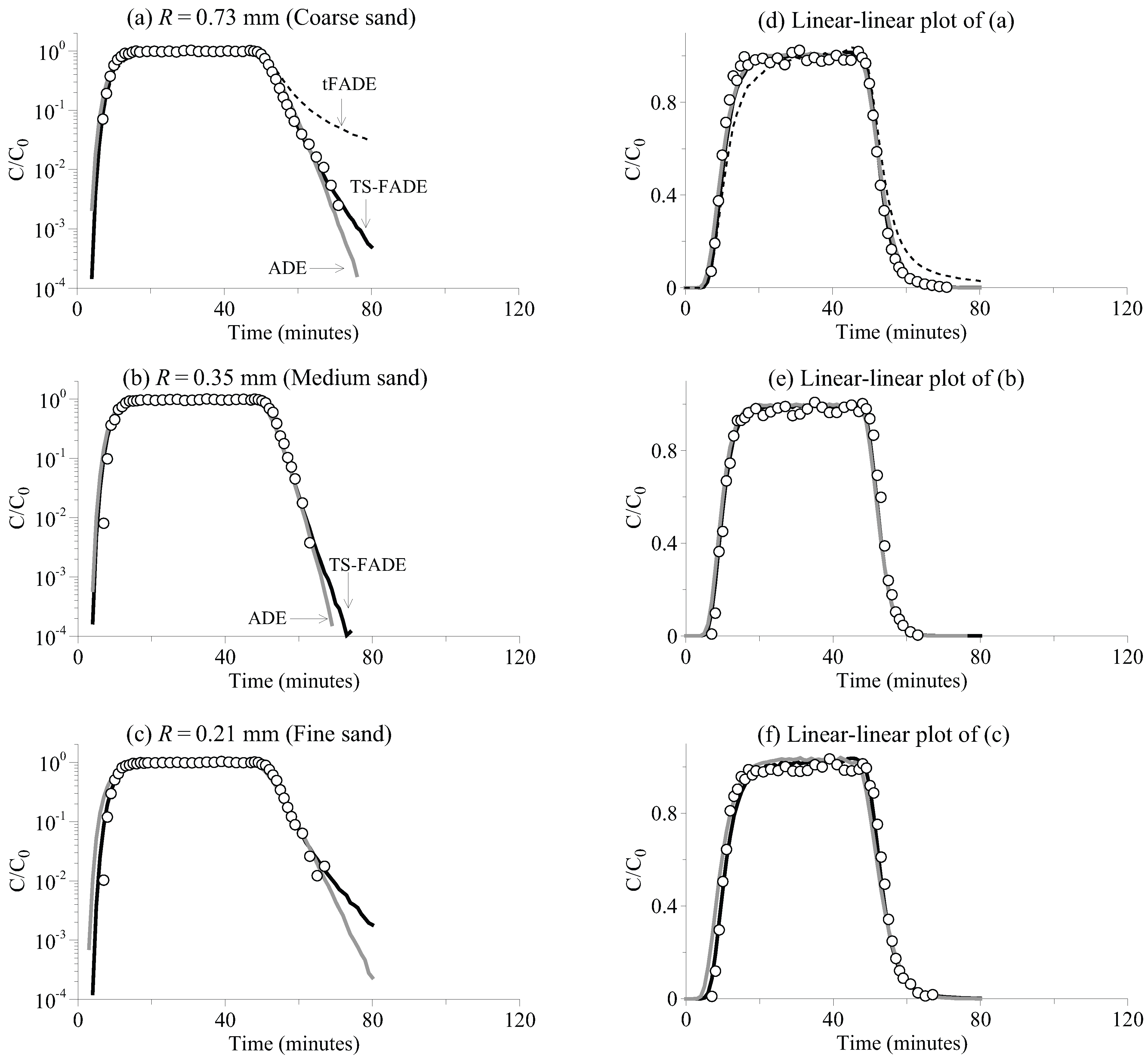
Figure 1.
The CuSO
breakthrough curves (BTC) along a 10 cm-long sand column: the measurements (symbols)
versus the best-fit solutions using the ADE model in Equation (
1) (grey lines), the time-fractional advection-dispersion equation (tFADE) model in Equation (
3) (the dashed line) and the TS-FADE model in Equation (
5) (black lines). In the legend, “
R” denotes the median grain size.
The measured CuSO
BTCs are shown in
Figure 1,
Figure 2 and
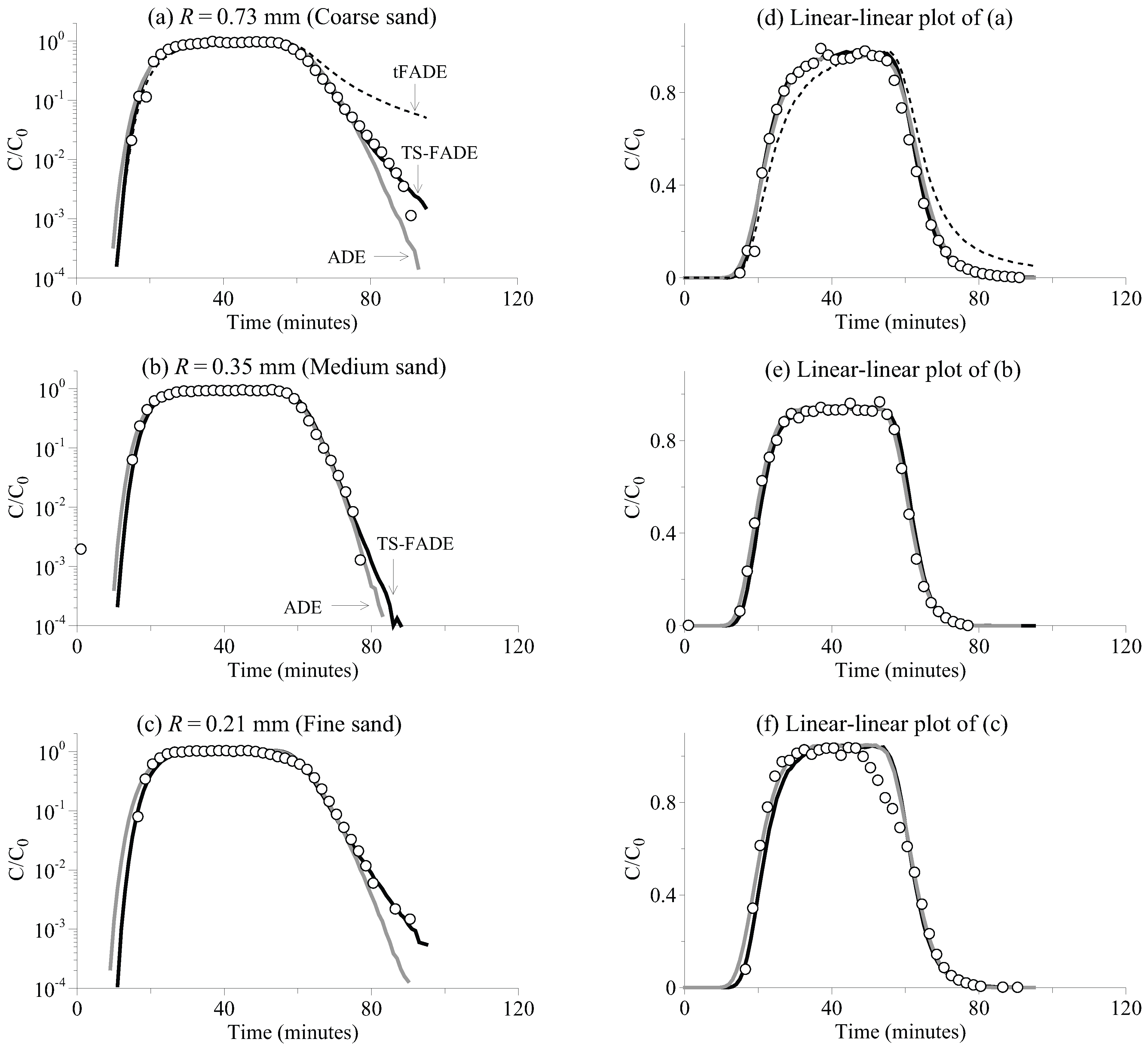
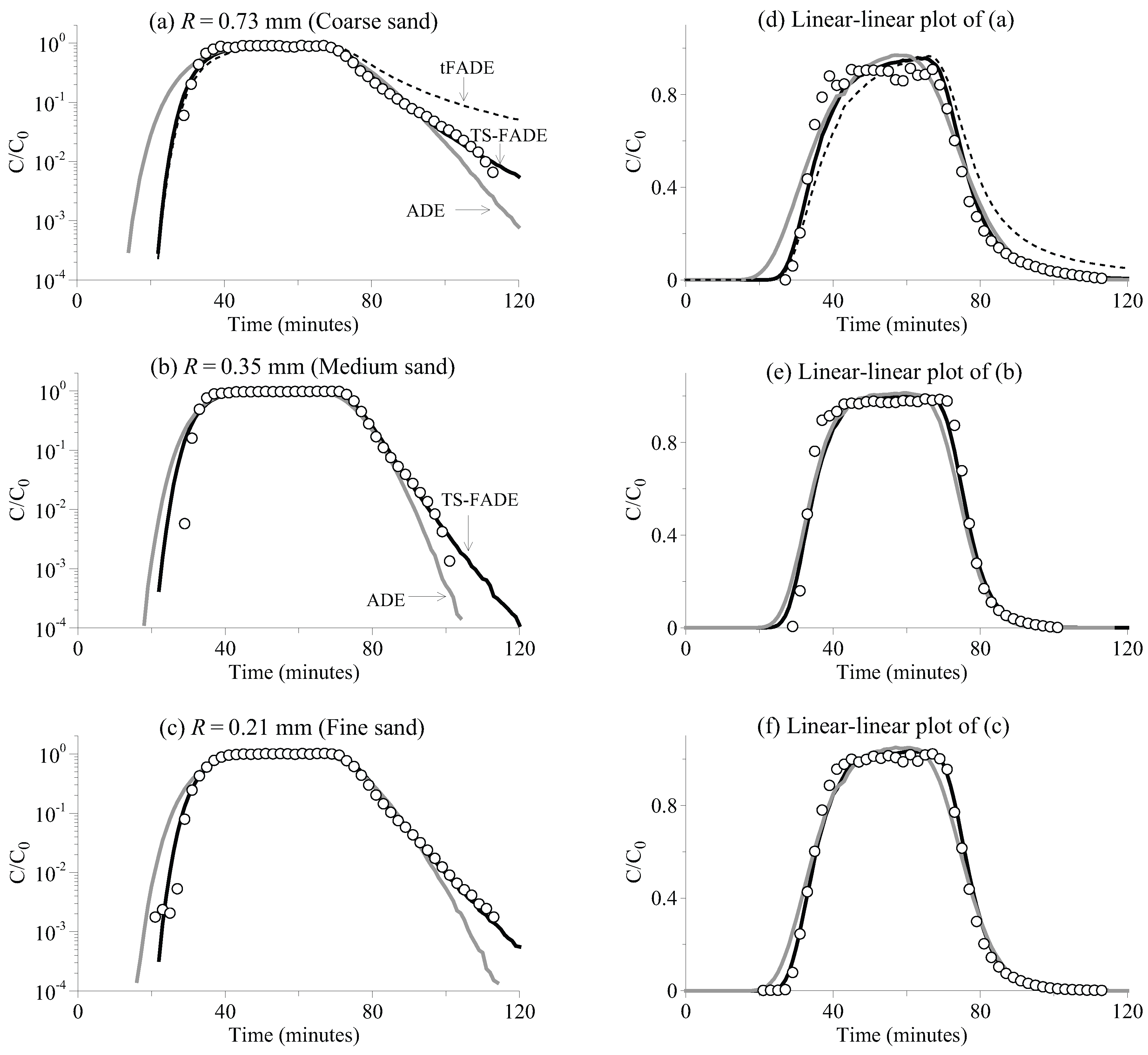
Figure 3, for the travel distance of 10 cm, 20 cm and 40 cm, respectively. The early time tails of all BTCs (representing the early arrivals of solute) are as steep as exponential, implying that there is no fast movement along preferential flow paths. This is expected, since super-diffusive transport typically requires a heterogeneous medium with a hydraulic conductivity field exhibiting large correlation length and variance [
9]. The late-time tails of BTCs, however, become relatively heavier with an increase of the travel distance. In the next section, we conduct numerical analysis to reveal whether the observed transport is actually scale-dependent.
Figure 2.
The CuSO
BTC along a 20 cm-long sand column: the measurements (symbols)
versus the best-fit solutions using the ADE model in Equation (
1) (grey lines), the tFADE model in Equation (
3) [the dashed lines in (
a) and (
d)] and the TS-FADE model in Equation (
5) (black lines).
Figure 2.
The CuSO
BTC along a 20 cm-long sand column: the measurements (symbols)
versus the best-fit solutions using the ADE model in Equation (
1) (grey lines), the tFADE model in Equation (
3) [the dashed lines in (
a) and (
d)] and the TS-FADE model in Equation (
5) (black lines).
Figure 3.
The CuSO
BTC along a 40 cm-long sand column: the measurements (symbols)
versus the best-fit solutions using the ADE model in Equation (
1) (grey lines), the tFADE model in Equation (
3) (the dashed lines in (
a) and (
d)) and the TS-FADE model in Equation (
5) (black lines).
Figure 3.
The CuSO
BTC along a 40 cm-long sand column: the measurements (symbols)
versus the best-fit solutions using the ADE model in Equation (
1) (grey lines), the tFADE model in Equation (
3) (the dashed lines in (
a) and (
d)) and the TS-FADE model in Equation (
5) (black lines).
4. Discussion
4.1. Short-Duration of Normal Diffusion in Relatively Homogeneous Porous Media
The above laboratory and numerical tests reveal that normal diffusion may only exist for a short travel distance (
i.e.,
cm) in the relatively homogeneous sand columns. The short-duration of normal diffusion may be due to two reasons. First, there may be small-scale variations in the packing of the sands, which leads to micro-structure (such as aggregates) in the macroscopic homogeneous medium. The silica sand used in our experiments is not perfectly uniform, but has a relatively narrow size distribution, which also helps to build internal structures. Solute particles diffusing into the sand matrix or a dead-end water zone may be delayed and, therefore, build the late-time tail of the BTC. If the transport is a non-dissipative process, the microscopic scale heterogeneity may control the macroscopic dynamics [
30]. With an increase of the spatial scale, more (and perhaps larger) aggregates may be formed, and the solute transport is delayed further, resulting in scale-dependent sub-diffusion. It is well-known that the solute particle jumps can be regarded as instantaneous [
1], and hence, the clock time [expressed, for example, by Equation (
4b)] between jump events represents the random waiting time for random-walking particles. At a small scale in both space and time, most particles have not experienced large retention periods yet, and the transport exhibits initial behavior similar to normal diffusion. Normal diffusion, therefore, may only be an approximation of real-world anomalous diffusion at a small spatiotemporal scale where the anomaly has not apparently developed yet.
Another explanation is the fractal geometry of silica sand (see, for example, [
31,
32], among others), which tends to generate anomalous diffusion. This explanation, however, is difficult to validate directly. Some researchers also argued that the fractal properties of soil might not be so obvious [
30]. The qualitative link between fractal properties of sand (such as texture and surface area) and fractional dynamics remains to be shown [
33]. In addition, a recent study [
34] found that uniform glass beads (which may contain aggregates or relatively immobile flow zones when they are packed in glass tubes) without any multi-fractality can also lead to sub-diffusion.
It is noteworthy that the limited duration of normal diffusion may be even shorter in natural geological formations with intrinsic multi-scale heterogeneity. Mixing and structured sands in the field can enhance (i.e., super-diffusion) or decelerate (i.e., sub-diffusion) the motion of solute particles, which can appear much earlier than those in the laboratory sand columns.
The short-duration of normal diffusion challenges the ADE-based hydrologic modeling, with one example discussed blow.
4.2. Challenge on the Definition of the Representative Element Volume
The scale-limited normal diffusion constrains seriously the size of the representative elementary volume (REV) [
35]. The conventional local ADE is believed to be applicable at the scale of REV, so that the heterogeneity of a large-scale medium must be adequately represented at the REV scale. For a regional scale (
i.e., kilometers) model, the size of each homogeneous cell is usually larger than one meter, which is at least one order of magnitude larger than the valid scale of normal diffusion revealed by this study. A finer resolution with a small REV, however, can lead to a prohibitive computational burden.
Several recent studies also identified a very small REV or even could not find the scale for REV. For example, Yoon and McKenna [
36] found that the REV may exist at the length of 0.25 cm, while local-heterogeneity features below the REV should still be quantified in numerical modeling. Klise
et al. [
37] conducted an unprecedented laboratory experiment by taking a thin slab of Massillon sandstone and exhaustively sampling the permeability (
k) via air permeability sampling. The
cm slab was measured for
k every 0.33 cm, yielding 17,328 measurements. Each sample support volume was on the order of 0.45 cm
. The finely discretized ADE, however, could not capture the observed early or late time tails of the tracer BTC [
37]. Major
et al. [
38] further found that sub-grid dispersion (below the support volume) is non-Fickian, and the non-local transport model is needed to capture the observed transport.
4.3. Fractional Dynamics for Tracer Transport in Relatively Homogeneous Sand Columns
The underlying dynamics for tracer transport in relatively homogeneous sand columns is transient sub-diffusion, due to probably the physical and chemical properties in the transport process. The finite retention capacity of sand matrix, probably due to the limited thickness of matrix and the non-negligible diffusive displacement of solute [
39], acts as an upper bound for tracer particle waiting times. This is similar to what we observed in solute retention in alluvial aquifers [
39]. Fractional dynamics in porous media therefore may depend on both the physical properties of the media and the chemical properties of the tracer.
The waiting time for solute particles between jump events exhibits multi-fractal scaling, which evolves in space. Numerical fitting in
Section 3.3 shows that the particle waiting time distribution at a given spatial scale is a power-law function transferring gradually to become exponential. According to [
40], multi-fractality can arise from a linear, additive process, whose increments have power-law tails with a variable truncation. Note that, here, the multi-fractal waiting times also grow in space, since the tempering parameter,
λ (which defines the rate of exponential tempering of the power-law tail), changes with the travel distance.
4.4. Factors Affecting Sub-Diffusion in Relatively Homogeneous Sand Columns
In our experiments, the spatial scale affects the tempering parameter,
λ, but the time fractional order,
γ (which is also the BTC or waiting-time tail index), remains stable in these uniformly packed sand columns. For a given tracer, the index,
γ, is a non-local parameter characterizing the overall retention capacity of the medium. In general, a stationary medium with strong immobile regions may be characterized by a small, constant
γ [
9]. The tempering parameter,
λ, on the other hand, records the extreme retention event, which, therefore, may change with the local variation of immobile zone properties.
In addition, the sand size also significantly affects the tailing behavior of transport, which can also be captured by adjusting the tempering parameter in the TS-FADE model in Equation (
5). For coarse and medium sand,
λ decreases with an increase of the travel distance (see
Table 1). For fine sand, however,
λ fluctuates with the spatial scale, where the relative amplitude of fluctuation is smaller than that for the coarser sand. The discrepancy might imply that the immobile zones formed by fine sand have relatively less variability (such as properties of segregates) than that for coarser sands. This hypothesis needs further experimental and numerical tests in a future study.
It is noteworthy that, for a short travel distance in relatively homogeneous media, the parameters in the TS-FADE model in Equation (
5) may not be unique when fitting the measured BTC. This is because the late-time tailing of transport cannot fully develop in a limited time; see, for example,
Figure 1c. Even if the observation time is long enough to capture the full range behavior of late-time tailing, the measured BTC may still remain incomplete, due to the concentration detection limit of tracers. Caution is therefore needed when quantifying a small-scale transport using the TS-FADE model in Equation (
5).
4.5. Possible Influence of the Small Diameter of the Sand Columns on Anomalous Diffusion
The repacked sand columns in this study have a relatively small diameter (25 mm), which may affect solute transport in three ways. First, a narrower column may force sand to be packed tightly, resulting in more dead zones for flow that can enhance the trapping of solutes. Second, solute particles may be trapped between the narrow glass tube and the filled sands, and solutes may also sorb on to the glass tube. Third, a narrower sand column provides less spatial inter-connectivity that is necessary for super-diffusion. The first two impacts tend to enhance sub-diffusion, while the last one may constrain the generation of super-diffusion.
Further analysis, however, shows that the above possible impacts might be minimized in this study. For example, for a short column (
Figure 1), the classical ADE model captures the observed BTCs, showing that the narrow sand column with a short length does not necessarily cause sub-diffusion. In addition, although none of the observed BTCs exhibit heavy early-time tails (the BTC with a power-law early-time tail is one of the typical characteristics of super-diffusion), this does not mean that the sand column with a small diameter must constrain super-diffusion. Previous studies, such as Herrick
et al. [
41] and Kohlbecker
et al. [
42], showed that the heavy-tailed and long-range-dependent hydraulic conductivity (
K) field is needed to generate heavy-tailed solute displacement. In this study, the repacked silica-sand columns do not contain such a heterogeneous
K field. Indeed, to the best of our knowledge, no previous studies showed that the column experiments packed with relatively homogeneous sand can build heavy-tailed super-diffusive transport. Therefore, the small diameter of the sand columns may have limited impact on the anomalous transport observed in this study. We will check this hypothesis in a future study, by using glass tubes with various inner diameters. Additional factors, such as variable-density flow and undisturbed soils may also be considered to explore the possible influence of the lateral dimension of sand columns on tracer transport.
It is also noteworthy that glass tubes with a centimeter-scale inner diameter have also been used to study various aspects of transport, especially in the last two years. For example, Ngueleu
et al. [
43] used a glass column with an inner diameter of 24 mm (and a length of 150 mm) to minimize the sorption of lindane onto the equipment. Sagee
et al. [
44] conducted column experiments for silver nanoparticle transport in closed, cylindrical columns with an inner diameter of 31 mm (and a length of 100 mm). Gouet-Kaplan
et al. [
45] packed sands in an acrylic vertical column with an internal diameter of 30 mm (to a height of 150 mm) to study the mixture of water. Zhang
et al. [
34] measured bromide transport through a horizontal glass tube with internal dimensions of 15.9 mm (diameter) (and 150 mm in length). Historic and well-known column experiments also used columns with similar sizes. For example, Gramling
et al. [
46] monitored bimolecular reactions through a thin glass chamber with the smallest thickness being 18 mm. Raje and Kapoor [
47] measured reactive kinetics across a glass column with a diameter of 45 mm (and a length of 180 mm). We also emphasize that the focus of the above column experiments differs from this study.
4.6. Reason to Select the Fractional Models with Temporal Derivatives
The introduction of the time-fractional derivative in Equations (
3) and (
5) is motivated by the observed late time tailing of BTCs. Other time-nonlocal transport models can also capture the delayed transport, including the well-known multi-rate mass transport (MRMT) model [
48] and the continuous time random walk (CTRW) framework [
10], which have been used widely by the hydrologic community. The time-fractional derivative models in Equations (
3) and (
5), which can describe the time nonlocal transport processes, such as sub-diffusion, are specific and simplified MRMT models with power-law distributed mass exchange rates. Model in Equation (
5) may also be functionally equivalent to the CTRW framework with a truncated power-law memory function in Equation [
10], and model in Equation (
5) requires fewer parameters (e.g., only the tempering parameter,
λ) to capture the nuance of an exponentially truncated power-law tail in the BTC. Discrepancy between fractional models and the other time-nonlocal models is not the main focus of this study. We leave this discussion for future work.
The transport process observed in this study is not super-diffusive, but sub-diffusive, since the late time tailing of BTC suggests a retardation process (a typical behavior of sub-diffusion), and there is no sign of fast displacement for CuSO
. This process might not be related obviously to the small diameter of the sand columns, since the sand column with a much larger diameter (
i.e., 300 mm) can also lead to sub-diffusion (see, for example, [
49]), and the above discussion implies the minimal impact of column diameter on transport.
It is noteworthy that we did not use the fractional models with spatial derivatives, since they describe processes different from our observations. Particularly, the space fractional advection-dispersion equation with maximally positive skewness captures super-diffusion with heavy power-law early-time tails in BTCs [
9], which is not observed in our column experiments. The space fractional advection-dispersion equation with maximally negative skewness does capture sub-diffusion, but the solute particles must travel backward and reach the upstream boundary [
9]. This power-law backward movement is not apparent, if not impossible, in our laboratory tests.
5. Conclusions
This study evaluates the dynamics of nonreactive tracer transport in relatively homogeneous media. The fundamental assumption in typical hydrologic models is that normal diffusion in homogeneous cells is scale-independent. To check this assumption, we conducted laboratory transport experiments and explored whether the dynamics of CuSO transport through silica sand columns varies with the travel distance. The measured BTCs were then interpreted using both the standard ADE model and the fractional-derivative models. The combined study of laboratory tests and stochastic analysis leads to the following three major conclusions.
(1) Normal diffusion and the representative element volume are only valid at small scales.
(2) The TS-FADE model can capture the scale-dependent sub-diffusive transport through relatively homogeneous media.
(3) The tempering parameter in the TS-FADE model generally decreases with an increase of the column length (due probably to the higher probability of long retention precesses), while the time index (which is a non-local parameter) remains stable.


