
Self-Calibration of UAV Thermal Imagery Using Gradient Descent Algorithm


1
Faculty of Physics and Applied Computer Science, AGH University of Krakow, 30-059 Krakow, Poland
2
Institute of Meteorology and Water Management—National Research Institute, 01-673 Warszawa, Poland
*
Author to whom correspondence should be addressed.
Drones 2023, 7(11), 683; https://doi.org/10.3390/drones7110683
Submission received: 30 September 2023
/
Revised: 16 November 2023
/
Accepted: 17 November 2023
/
Published: 20 November 2023
(This article belongs to the Special Issue Unmanned Aerial Vehicles in Atmospheric Research)
Abstract
:Unmanned aerial vehicle (UAV) thermal imagery offers several advantages for environmental monitoring, as it can provide a low-cost, high-resolution, and flexible solution to measure the temperature of the surface of the land. Limitations related to the maximum load of the drone lead to the use of lightweight uncooled thermal cameras whose internal components are not stabilized to a constant temperature. Such cameras suffer from several unwanted effects that contribute to the increase in temperature measurement error from ±0.5 °C in laboratory conditions to ±5 °C in unstable flight conditions. This article describes a post-processing procedure that reduces the above unwanted effects. It consists of the following steps: (i) devignetting using the single image vignette correction algorithm, (ii) georeferencing using image metadata, scale-invariant feature transform (SIFT) stitching, and gradient descent optimisation, and (iii) inter-image temperature consistency optimisation by minimisation of bias between overlapping thermal images using gradient descent optimisation. The solution was tested in several case studies of river areas, where natural water bodies were used as a reference temperature benchmark. In all tests, the precision of the measurements was increased. The root mean square error (RMSE) on average was reduced by 39.0% and mean of the absolute value of errors (MAE) by 40.5%. The proposed algorithm can be called self-calibrating, as in contrast to other known solutions, it is fully automatic, uses only field data, and does not require any calibration equipment or additional operator effort. A Python implementation of the solution is available on GitHub.
1. Introduction
The cost efficiency and flexibility of high-resolution thermal imagery from UAVs are advantages for environmental monitoring and management. UAV-based thermal and narrowband multispectral imaging sensors meet the critical requirements of spatial, spectral, and temporal resolutions for vegetation monitoring [1]. UAVs provide high spatial resolution and flexibility in data acquisition and sensor fusion, allowing for land cover classification, change detection, and thematic mapping [2]. Aerial thermography from low-cost UAVs can be used to generate digital thermographic terrain models, which find application in the classification of land uses according to their thermal response [3]. Thermal remote sensing has many potential applications in precision agriculture, including monitoring plant hydration levels, identifying instances of plant diseases, evaluating crop yield, and analysing plant characteristics [4]. Another area of application is related to hydrology, where thermal images can be used to locate and quantify discrete thermal inputs to rivers [5,6,7].
Limitations related to the maximum load of the UAV as well as cost constraints lead to the use of mainly lightweight uncooled thermal cameras. This solution has several shortcomings when measuring temperature under field conditions. Uncooled UAV thermal cameras require careful calibration and correction for various factors to obtain accurate temperature measurements. They suffer from vignette effects, sensor drift, ambient temperature and solar radiation influences, and measurement bias, which can be corrected with an ambient temperature-dependent radiometric calibration function [8]. Non-radiometric uncooled thermal cameras are highly sensitive to changes in their internal temperature and require empirical linear calibration to convert camera digital numbers to temperature values [9]. Fluctuations in the temperature of the focal plane array (FPA) detector, wind, and irradiance can affect temperature measurements, and adequate settings of camera gain and offset are crucial to obtaining reliable results [10]. Uncooled thermal cameras also suffer from thermal-drift-induced nonuniformity or vignetting [11]. The above factors contribute to the deterioration of the camera’s accuracy from ±0.5 °C in laboratory conditions to ±5 °C in unstable UAV flight conditions [9].
The literature provides a number of solutions to reduce this problem. To minimise measurement errors in UAV thermal cameras, it is suggested that the camera is warmed up for 15–40 min before starting the actual measurement [9,11]. There are also several methods to eliminate unwanted phenomenon outcomes with calibration under controlled conditions. For example, calibration algorithm based on neural networks can be used to increase measurement accuracy [12]. Vignetting reduction can be achieved using reference images of a homogeneous target [11]. Ambient temperature-dependent radiometric calibration function can be used to correct for sensor drift, ambient temperature influences, measurement bias, and vignette effects [8]. Stabilization of the camera response and fixed pattern nose removal can be achieved with advanced radiometric calibration [13]. The disadvantage of calibration-based methods is that they require non-standard equipment and the extra effort needed to collect calibration data. A correction based only on the field data collected by the UAV system would be favoured. Such an approach can be referred to as self-calibration (a term that originated from the field of photogrammetry, where it is defined as a process that “uses the information present in images taken from an un-calibrated camera to determine its calibration parameters” [14]). Such a method for bias correction using redundant data from overlapping areas of aerial thermal images has been proposed [15]. It is based on mathematical modelling of the metric of “variation of digital number per second”. Unfortunately, despite good results, the authors did not provide a specific explanation, formula, or sample source code illustrating the calculation of this metric. Also, since this method leverages the rate of digital number variation, it requires precise timing of the image acquisition achieved with a custom drone attachment. Often by default, the time information available in the image metadata is provided with the precision of a second, which is not sufficient for rate of digital number variation calculation, as during the flight, successive photos are taken even as often as about every 1 s.
Another important aspect of the problem is the lack of specific details of algorithms used for processing of thermal images. The user has to rely on the producer’s closed-source Thermal SDK (software development kit) library for allowing to make corrections to the measurement by taking into account air humidity, target emissivity, or flight altitude. It is not known what exact processes are represented in this algorithm. Moreover, significant shortcomings of using SDK were noticed while conducting this study: (i) the maximum flight altitude acceptable by the library is 25 m, which is too low for most flights covering large areas, (ii) the library returns errors for some humidity values (most often for a relative humidity of about 60%), and (iii) for a given frame, it is possible to select only one emissivity (it is not possible to set different emissivities for different objects in the same photo). However, most of the UAV-dedicated cameras are susceptible to adverse phenomena typical of uncooled thermal cameras (bias, vignette effect).
The above-mentioned issues can be addressed by investigating redundant data from overlapping areas of the images. It is desirable that the temperature difference between all pairs of overlapping images be as small as possible. This is a minimisation problem that can be solved with any optimisation method. This work focuses on the use of gradient descent, which is an optimisation algorithm commonly used in machine learning. However, beyond its main application in machine learning, gradient descent can be used to optimise any differentiable objective function.
Gradient descent works by iteratively updating a set of parameters in the direction of the steepest descent of a cost function. The algorithm computes the gradient of the cost function with respect to the parameters and then updates the parameters by taking a step in the direction of the negative gradient. The learning rate parameter determines the size of the step, and it is usually set to a small value to avoid overshooting the minimum of the cost function. The algorithm continues to iterate until the cost function converges to a minimum or a stopping criterion is met. With the popularity of machine learning, gradient descent has become more accessible thanks to the development of software libraries that accelerate the algorithm by using the GPU (graphical processing unit). This work will use the gradient descent ADAM optimisation method [16].
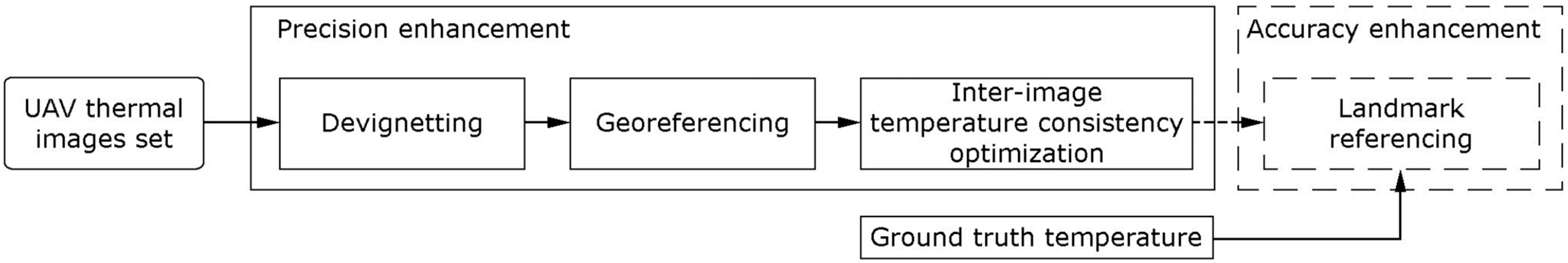
The aim of this work is to develop a method for post-processing of aerial thermal imagery that reduces the effects of undesirable phenomena occurring in uncooled thermal cameras without the use of non-standard equipment, such as reference black bodies or custom UAV attachments, and without access to raw thermal sensor data. The method consists of four steps (see Figure 1).
The following steps are responsible for:
- Devignetting—reduction of temperature pixel bias within each single picture caused by non-uniform temperature of the thermal sensor;
- Georeferencing—assigning the consistent coordinate system for the whole picture set based on EXIF (exchangeable image file format) metadata and characteristic keypoints identified on each picture;
- Inter-image temperature consistency optimisation—reduction of average temperature difference in the same areas recorded on different pictures;
- Landmark referencing—minimising the temperature offset of the whole thermal mosaic based on ground-based reference points.
The first three steps are dedicated to precision enhancement and can be used independently of the last one. The purpose of the last step is to improve the accuracy of the thermal map by eliminating the difference between the temperature of a selected point obtained from the thermal camera and the ground truth temperature measured directly on the surface. It is recommended to perform at least three reference measurements [9,17].
Achieving this goal is important, as the use of thermal imaging cameras is becoming widespread but proven post-processing methods are lacking.
2. Materials and Methods
2.1. Data
The thermal pictures were collected by the DJI Matrice 300 RTK drone system equipped with a Zenmuse H20T multicamera sensor that contains the thermal camera. Photos were captured from an altitude of 50 m with the side and front overlapping with a factor of 80%. The emissivity value of 0.95 was used based on a series of laboratory experiments performed in controlled conditions using the same thermal camera that was applied in the field. Data used in this study were collected from several areas in southern Poland:
- Area around about 500 m of the Kocinka stream stretch near Grodzisko village (50.8715 N, 18.9661 E);
- Area around about 350 m of the Kocinka stream stretch near Rybna village (50.9371 N, 19.1134 E);
- Area around about 160 m of the Sudół stream stretch near Kraków city (50.0999 N, 19.9027 E).
The water temperature of the rivers was measured using a thermocouple along their course in each case. The results were constant for the entire section and did not depend on chainage. Table 1 provides details of the locations, dates, conditions of the surveys, and measured river water temperatures.
2.2. Algorithm
2.2.1. Devignetting
The correction of the vignette effect was conducted using the “single image” method [18]. “Single image“ means that the algorithm tries to model the correction of the vignette effect only on the basis of the currently processed image and does not have any auxiliary data available (e.g., an image of a homogeneous target with a clearly visible vignette effect). It was implemented by translating the MATLAB code available at https://github.com/GUOYI1/Vignetting_corrector (accessed on 18 June 2023) into Python. Several changes have been made to adapt the algorithm to work with thermal images. Standard images are represented with floating point values from 0 to 1 or integers from 0 to 255. The original implementation of the algorithm assumed this data format, so it had to be modified to work on unconstrained float values. Thermal image values can also be negative. The vignette correction algorithm works on logarithms of pixel values, so temperatures were converted to Kelvins in order to avoid the logarithm of 0. The vignette correction algorithm tends to increase the brightness of the photo. For standard photos, this is not an issue, but for thermal images, where increasing the brightness will result in a bias in the temperature reading, this cannot be accepted. It has been assumed that images with vignette effect occurrence contain more accurate temperatures in their central part. Therefore, the central part of the photo before correction has been used as a reference level for the photo obtained after applying the vignette correction algorithm. The bias is compensated for by subtracting the average difference between the central areas of the images before and after vignette correction. While the vignette effect mainly affects the edge part of the image, the central area size is defined as a rectangle with sides twice smaller than the whole image.
2.2.2. Georeferencing
The georeferencing algorithm is largely based on the aerial photo stitching solution proposed by Luna Yue Huang [19]. Modifications in the proposed method consists of direct georeferencing to the universal transverse mercator (UTM) coordinate system. The georeferencing of images can be done by any method or software that best suits the nature of the image set. It is important that georeferencing results in information about the overlapping areas between all pairs of images. It is not possible to precisely georeference a single photo showing a non-orthographic view, but the following georeferencing method proved sufficiently accurate for the proposed temperature calibration method.
The first part of the georeferencing procedure is initial georeferencing of images based on EXIF metadata. These contain information about the geographic coordinates, yaw, and altitude of the drone camera at the time the image was taken. This information, along with the angle of the field of view taken from the camera specifications, allows the estimation of an affine transformation parameters of translation (, ), scale (, ), and counter clockwise rotation () that allows to embed the image in a UTM coordinate system. This is not an accurate estimation, due to the low accuracy of the UAV’s GPS geolocation and high sensitivity to the shift of the camera viewing area under the influence of wind gusts. In this estimation, the scale and parameters are equal and the shear (, ) coefficients are 0. The elimination of shear parameters from the procedure was possible because the camera is equipped with the gimbal system controlling the nadir position of the camera during the flight. The transformation parameters allow to obtain the transformation matrix based on Equation (1).
Based on the initial georeferencing, pairs of overlapping images are found in the set. To ensure that all possible pairs are found even when errors in the initial georeferencing may indicate a lack of overlapping, footprints are expanded (buffered) by a dilation operation by the given padding value. Each pair of images is aligned and a relative transformation matrix is found by a well-established in the field of image vision stitching method: (i) finding corresponding points (so called keypoints) in both images using scale-invariant feature transform (SIFT) [20], (ii) matching keypoints using fast approximate nearest neighbour search (FLANN) [21], and (iii) estimation of best transformation matrix using random sample consensus (RANSAC) [22]. Relative transformations are verified in two stages: (i) since we assume that the images are taken from the same altitude (study areas are flat), the scaling factor in the relative transformation of two overlapping images must be approximately equal to 1. If the value of the scaling factor for relative transformations is outside the range 0.9–1.1, the relative transformation is considered incorrect. (ii) As all images are taken in the nadir orientation (gimbal camera positioning system), the relative transformations should not perform a shearing operation. When there is no shear, the absolute values of the relative transformation matrix satisfy the following condition: and . If deviation between these values is greater than 0.1, the relative transformation is considered to be incorrect. If the relative transformation is found to be incorrect, according to the Luna Yue Huang solution, an attempt is made to establish a relative transformation using the same pair of images, but resized to twice lower resolution. Such a procedure allows to obtain different keypoints for a scale determination. If the relative transformation obtained with this procedure also fails to pass verification, the analysed pair of images is discarded. Another possible procedure (in case of multisensory cameras) to overcome the relative transformation error is the use of higher resolution RGB pictures collected simultaneously with thermal; however, in this study, the procedure was focused on the possible application in case of single sensor thermal cameras.
Based on the verified pairs of images, an undirected graph is constructed [23], where each node is an aerial photo and each edge is a valid relative transformation between a given pair of images. The connected components are then extracted from the graph. A connected component in graph theory is a group of vertices in a graph that are all directly or indirectly connected to each other. Only images (nodes) from a connected component containing the largest number of nodes are used for further processing.
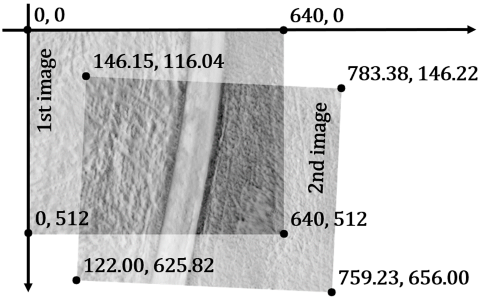
Coordinates of the second image corners are calculated in the pixel coordinate system of the first image of the pair using a relative transformation matrix :
where:
- —relative transformation matrix between the 2nd image and 1st image pixel coordinate systems;
- —coordinates of corner point expressed in the 2nd image pixel coordinate system;
- —coordinates of the same point expressed in the 1st image pixel coordinate system.
The procedure is repeated for each verified image pair from the set. The idea of this alignment procedure is visualised in Figure 2.
Optimisation of georeferencing of all images obtained during the flight involves tuning the absolute geographic transformation parameters (, , , , ) (for all images simultaneously) to make the relative transformations recovered from them as close as possible to the relative transformations obtained earlier using the alignment of each pair separately. Recovery of the optimised relative transformation matrix from the optimised absolute geographic transformation matrices and of two georeferenced images is obtained according to Equation (3):
and shear parameters are not tuned during the optimisation. Although tuning of these parameters improves the matching between pairs of photos further, it also introduces an unacceptable shearing of the entire mosaic of photos.
Similar to Equation (2), the coordinates of points expressed in the pixel reference system of the 2nd photo can be converted to coordinates expressed in the reference system of the 1st image using Equation (4):
where:
- —relative transformation matrix between the 2nd image and 1st image pixel coordinate systems after georeference optimisation;
- —coordinates of a point expressed in the 2nd image pixel coordinate system;
- —coordinates of the same point expressed in the 1st image pixel coordinate system after georeference optimisation.
Georeference optimisation is performed using the gradient descent method with the loss function that consists of two components and . Component is the mean Euclidean distance between the corner point coordinates obtained from the relative transformation recovered from the tuned absolute geographic transformation and the coordinates of the corresponding points that have been obtained from the relative transformation of the pair alignment procedure:
where:
- —number of pairs;
- —point of the j-th corner of the i-th pair of the 2nd image expressed in the 1st image pixel coordinate system estimated from pairs alignment;
- —point of the j-th corner of the i-th pair of the 2nd image expressed in the 1st image pixel coordinate system estimated using relative transformation recovered from absolute geographic transformations tuned during optimisation.
Component is the mean Euclidean distance between the geographic centroids of tuned image footprints and geographic centroids of image footprints obtained during initial georeferencing using EXIF data.
where:
- —number of images;
- —point of centroid of the i-th image obtained from EXIF data expressed in the geographic coordinate system;
- —point of centroid of the i-th image obtained from absolute geographic transformation tuned during optimisation.
By minimising the factor, the optimised absolute geographic transformations are adjusted, so that the relative transformations between images pairs that have been retrieved from them are as close as possible to the relative transformations previously obtained separately for each pair in the alignment process. Minimising the factor ensures that the entire mosaic will not move in any direction during the optimisation. Equation (7) is the final formula for the loss function. To minimise the impact on the relative matching of images using the component, the less important component is multiplied by a factor of . The factor value was selected experimentally by qualitative assessment of results tested for different values.
2.2.3. Inter-Image Temperature Consistency Optimisation
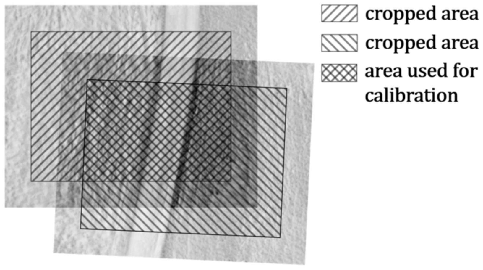
In order to minimise the temperature bias between overlapping images using gradient descent, a consistent dataset has to be prepared. If the reduction of the vignette effect has not yielded sufficient results and the photo overlap is large enough, the areas of the photos near the edges where the vignette effect affects the temperature images the most can be truncated (Figure 3).
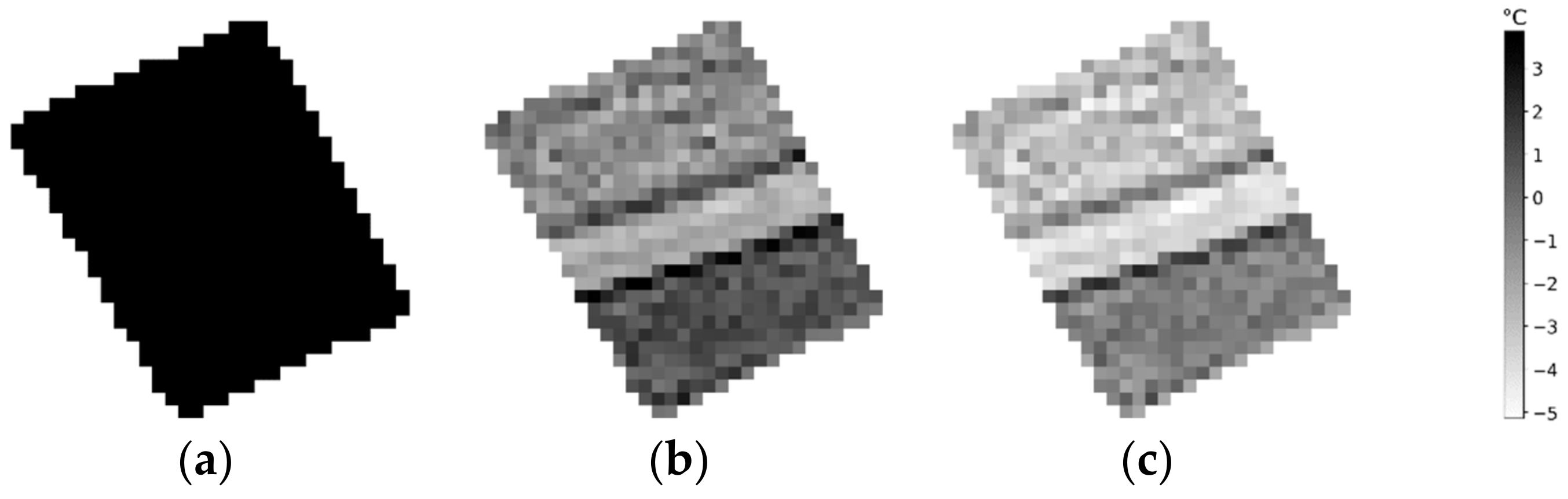
For the two images from each pair, only the common part is retained as well as a mask that allows to reproduce the irregular shape of the cut-out from the rectangular array. Temperature cut-outs of both images and the mask are resized to an array of pixels. During the resizing, the temperatures are interpolated using the bilinear method, and the mask is interpolated using the nearest neighbours method. The example result of the common clip is shown in Figure 4. The example corresponds to the image pair shown in Figure 2 and Figure 3. The rotation is due to the transformation to an absolute geographic datum. The lack of preservation of the aspect ratio is due to the need for scaling to fill the whole area of square array of pixels.
By resizing the slices to pixels, it was possible to create a coherent dataset of three arrays (the masks and the common parts of image pairs) of size , where is the number of pairs, which could then be used in optimisation using the gradient method.
Optimisation of the temperature values involves tuning the temperature offset between the calibrated and not calibrated image:
where:
- —temperature value with applied calibration;
- —temperature value before calibration.
Optimisation uses a loss function that consists of two components: and . Component is the pixelwise mean squared error between the calibrated temperature values of the first and second cut-out images from a given pair (Equation (9)):
where:
- —number of pairs;
- —calibrated temperature value of the pixel with the coordinates (j,k) of the 1st image in the i-th pair;
- —calibrated temperature value of the pixel with the coordinates (j,k) of the 2nd image in the i-th pair.
is the absolute difference between the mean values of temperatures in all uncalibrated and calibrated images (Equation (10)):
where:
- —mean temperature value of uncalibrated images;
- —mean temperature value of calibrated images.
By minimising the component, the bias between the temperature values in the overlapping images is minimised. The component ensure that during optimisation, the whole mosaic will not drift from the initial temperature mean value. The total loss is calculated using Equation (11). To minimise the impact of on bias correction using the component, the component was multiplied by factor of . The factor value was selected experimentally by qualitative assessment of results tested for different values.
2.3. Landmark Referencing
The rivers in the study areas have homogenous temperatures throughout the surveyed sections; therefore, the average of several dozens of temperature measurements performed along the river has been used for landmark referencing. The reference river measurements have been used to compensate a systematic error. The sets of both the original and temperature-adjusted images were shifted with the same offset value for all images from the given set, so that the average water body temperature read from the thermal mosaic was equal to the measured average reference water temperature. It was decided to apply this step because the temperature values returned by the DJI Thermal SDK may differ significantly from the actual temperature. This final landmark referencing step is optional, but it is a straightforward correction and makes it easier to compare measurement precision before and after the calibration procedure as it reduces a systematic error.
3. Results and Discussion
3.1. Devignetting
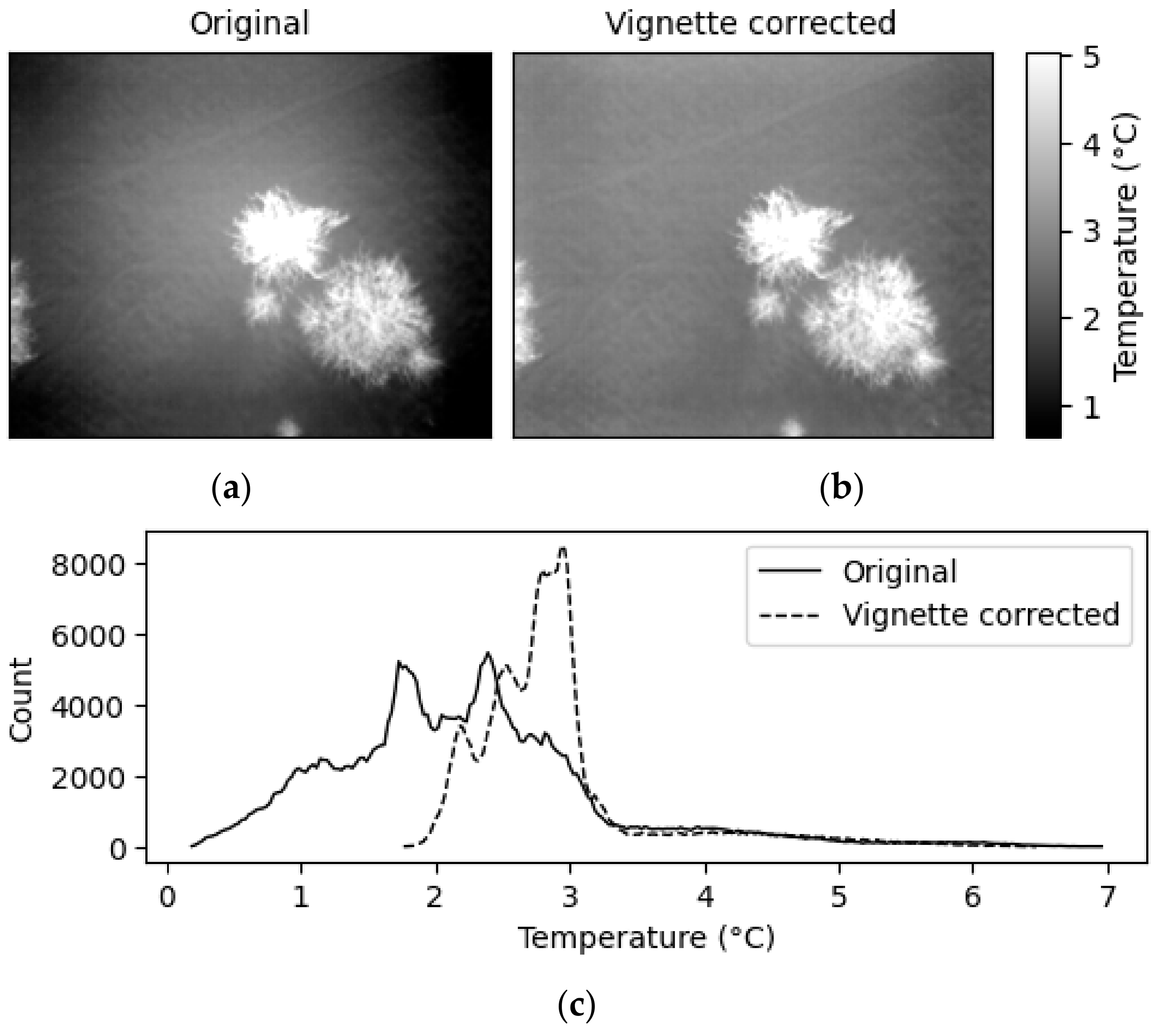
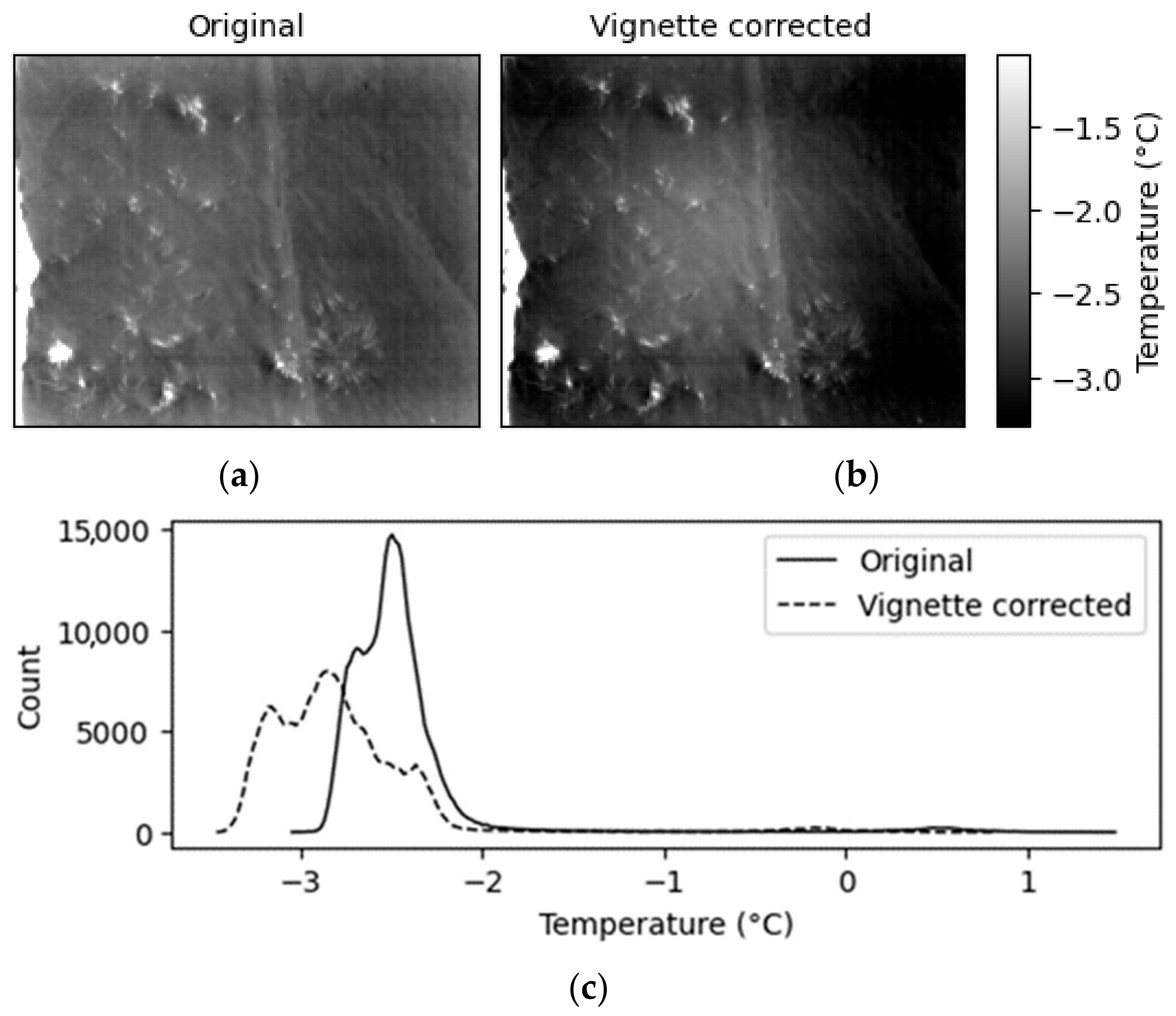
A ”single image” algorithm was used to correct the vignette effect. For this reason, the resulting image is prone to misinterpretations and consequently to an erroneous correction of the vignette effect. Figure 5 shows an example of a successful devignetting. In this case, the standard deviation of the temperature in the image decreased as a result of devignetting, which is manifested as a narrowing of the histogram of pixel temperature values. Figure 6 shows an erroneous devignetting, where it is likely that the river at the left edge of the image caused the misinterpretation. In this case, the correction resulted in an increase in the standard deviation of the image temperature, which manifests as a widening of the histogram of pixel values.
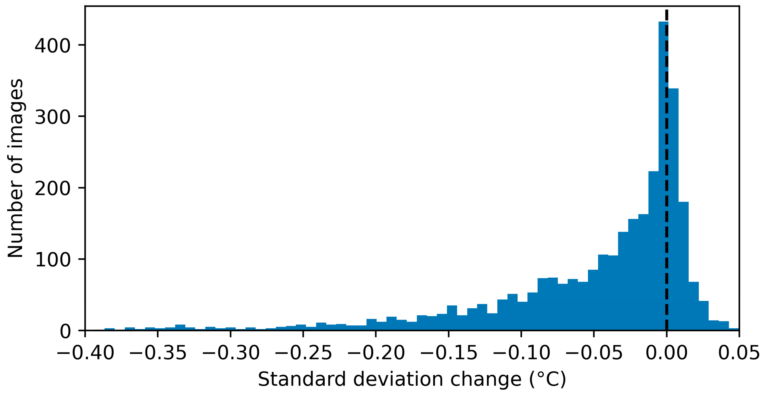
In order to assess the algorithm effectiveness quantitively, it was tested on a set of 3037 images. The measure of the algorithm effectiveness was a relative change in the image temperature standard deviation before and after the correction. For 74.4% (2261) of the images, a standard deviation reduction was obtained of –0.07 °C on average, and for 25.6% (776) of the images, an increase in the standard deviation was obtained of 0.01 °C on average. The detailed distribution of the changes in the temperature standard deviation as a result of the devignetting is shown in Figure 7.
3.2. Visual Assessment
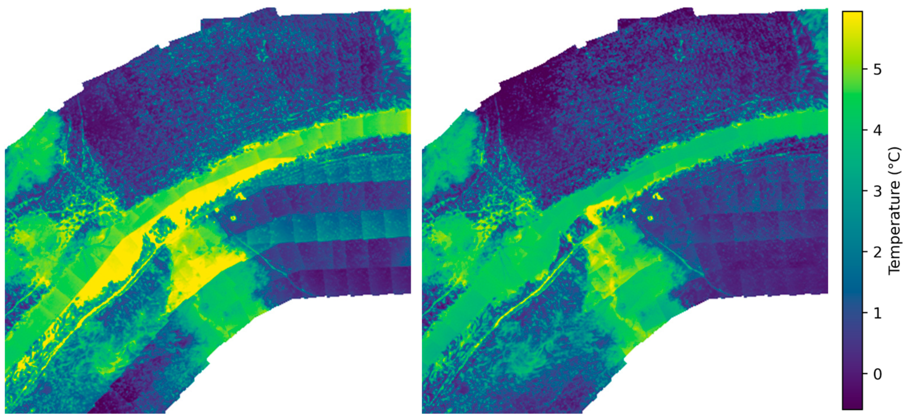
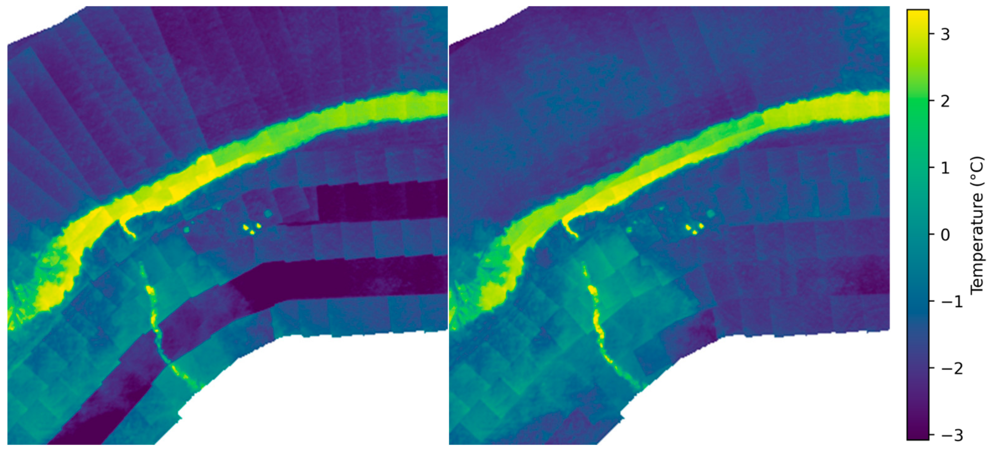
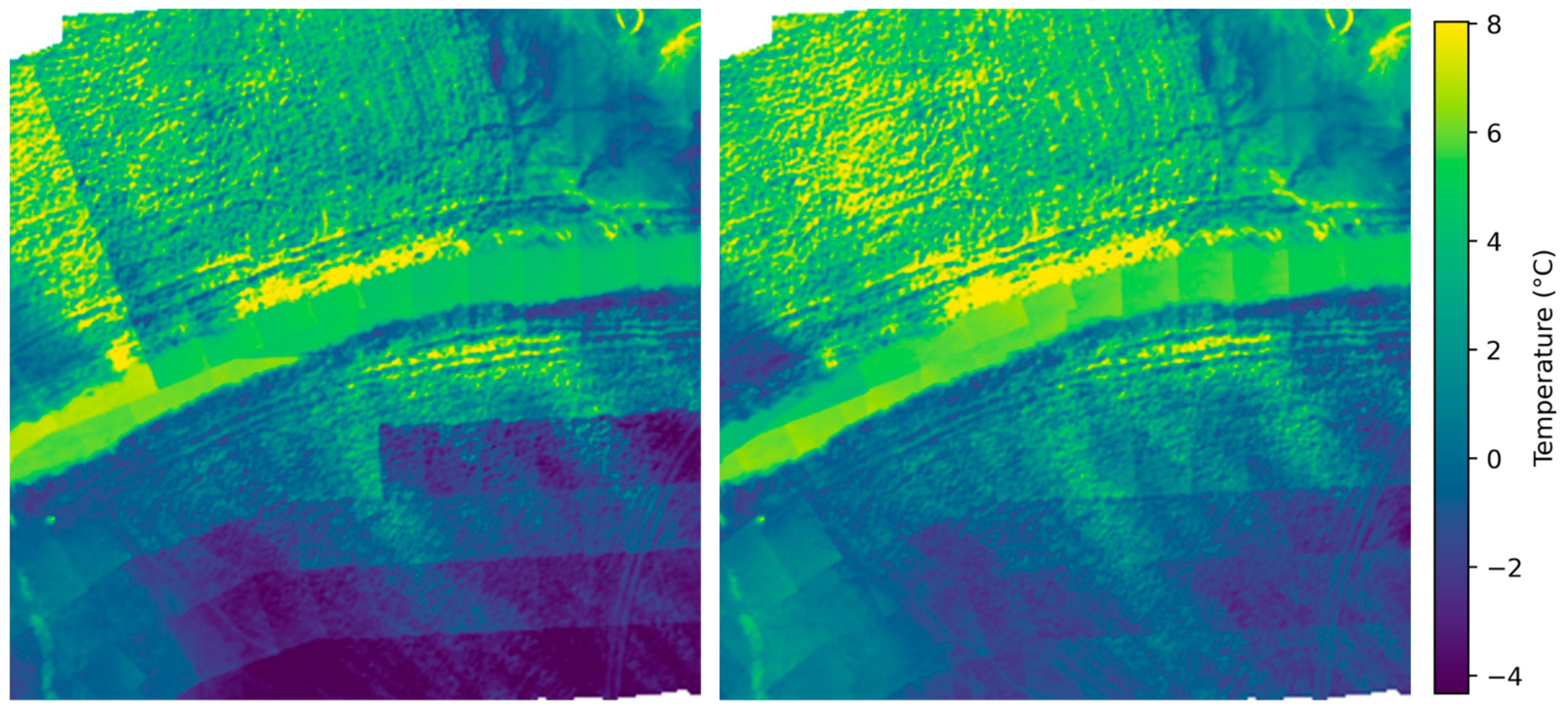
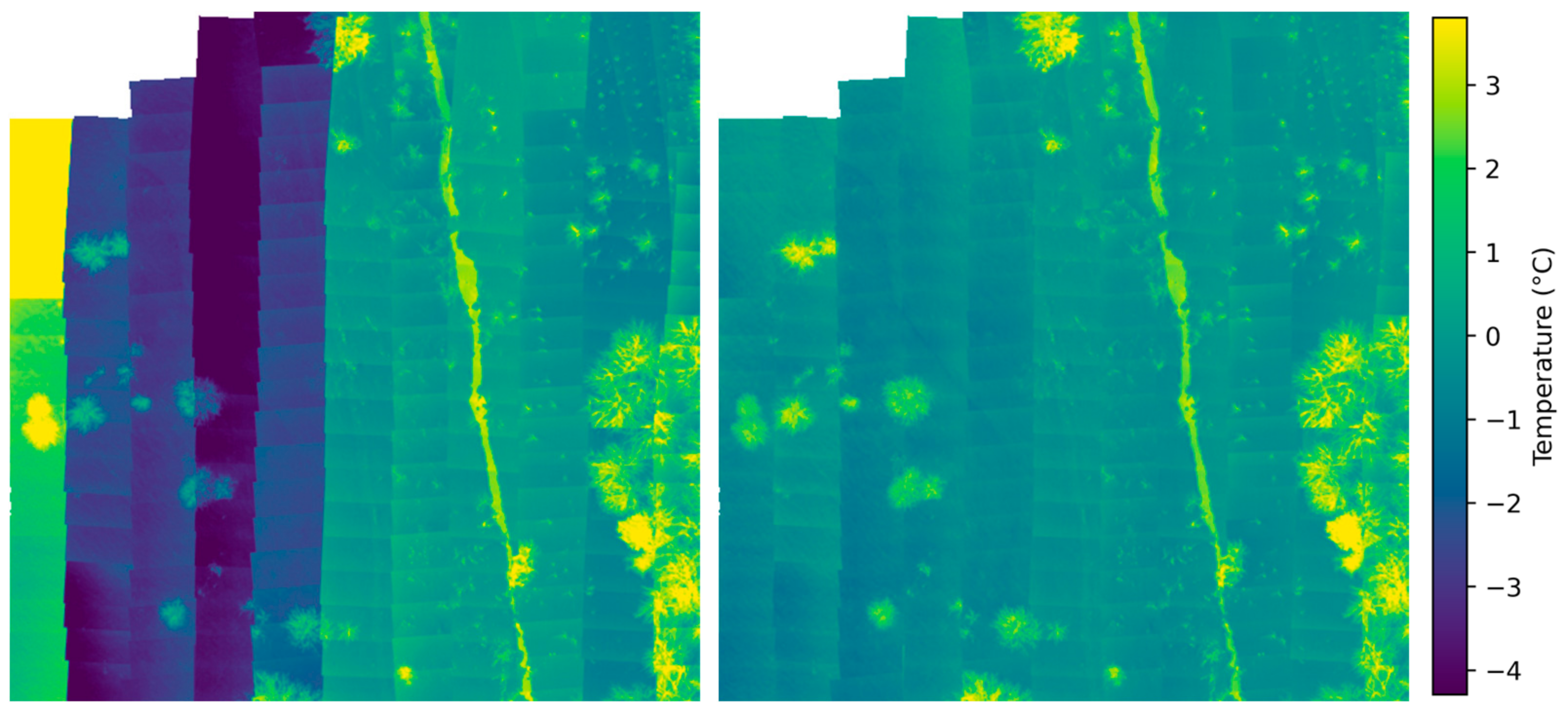
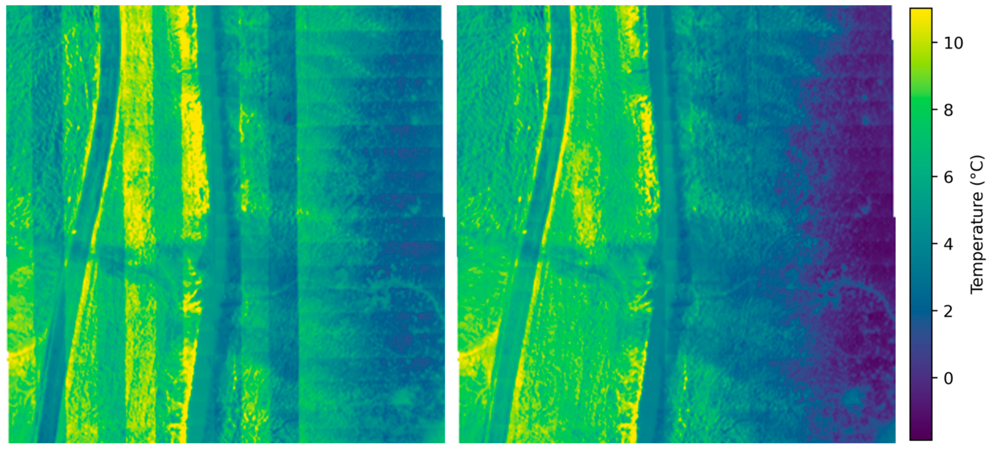
Figure 8, Figure 9, Figure 10, Figure 11 and Figure 12 show parts of thermal image mosaics before and after calibration for each case study (see Table 1). It should be noted that the pictures are not orthomosaics but image mosaics created straightforwardly by displaying all georeferenced images. If there was more than one image of the same area in a given set causing an overlap, a subsequent image was selected for the mosaic.
A visual comparison of the thermal imagery mosaics before and after calibration shows an improvement regarding the temperature fluctuations, particularly between successive flight passages that are noticeable as parallel bands in all of the uncorrected mosaics. The algorithm also handles the correction of undervalued images taken at the beginning of the flight when the camera is warming up, as seen, for example, in the left side of case D mosaic (Figure 11). Furthermore, correction of the images from the cases A (Figure 8) and B (Figure 9) has allowed to detect a warmer tributary of the stream, which is fed by the warm groundwater.
3.3. Waterbody Temperature
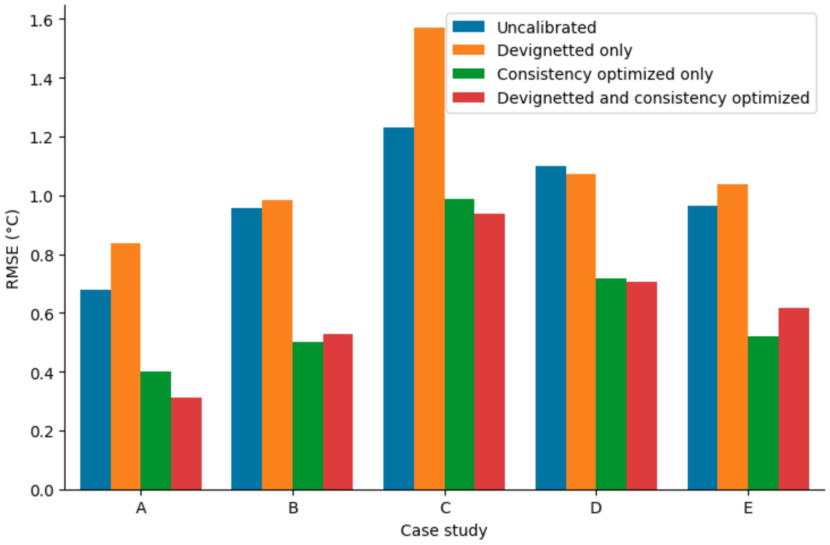
Figure 13 summarises the RMSE of river temperature measurements obtained from thermal images at various configurations of the calibration procedure: uncalibrated, devignetted only (Section 2.2.1), consistency optimised only (Section 2.2.3), and after applying both devignetting and consistency optimisation algorithms. To focus on the measurement precision only, all RMSE values (including uncalibrated) were calculated using images subjected to the landmark referencing described in Section 2.3.
Applying the devignetting algorithm itself resulted in an increase in RMSE in most cases, implying that the image temperature reading precision was decreased. A slight improvement was obtained in case D with a change in RMSE of –0.03 °C but it was statistically insignificant. Application of the inter-image consistency optimisation algorithm itself reduced the RMSE substantially in all cases, up to almost 50% in case B (from RMSE of 0.95 °C before the algorithm application down to 0.50 °C afterwards). Applying both algorithms to the image resulted in further improvement of the precision in three cases, and in the remaining two, the resulting RMSE increased compared to optimisation itself but was still substantially lower than that for the unprocessed image.
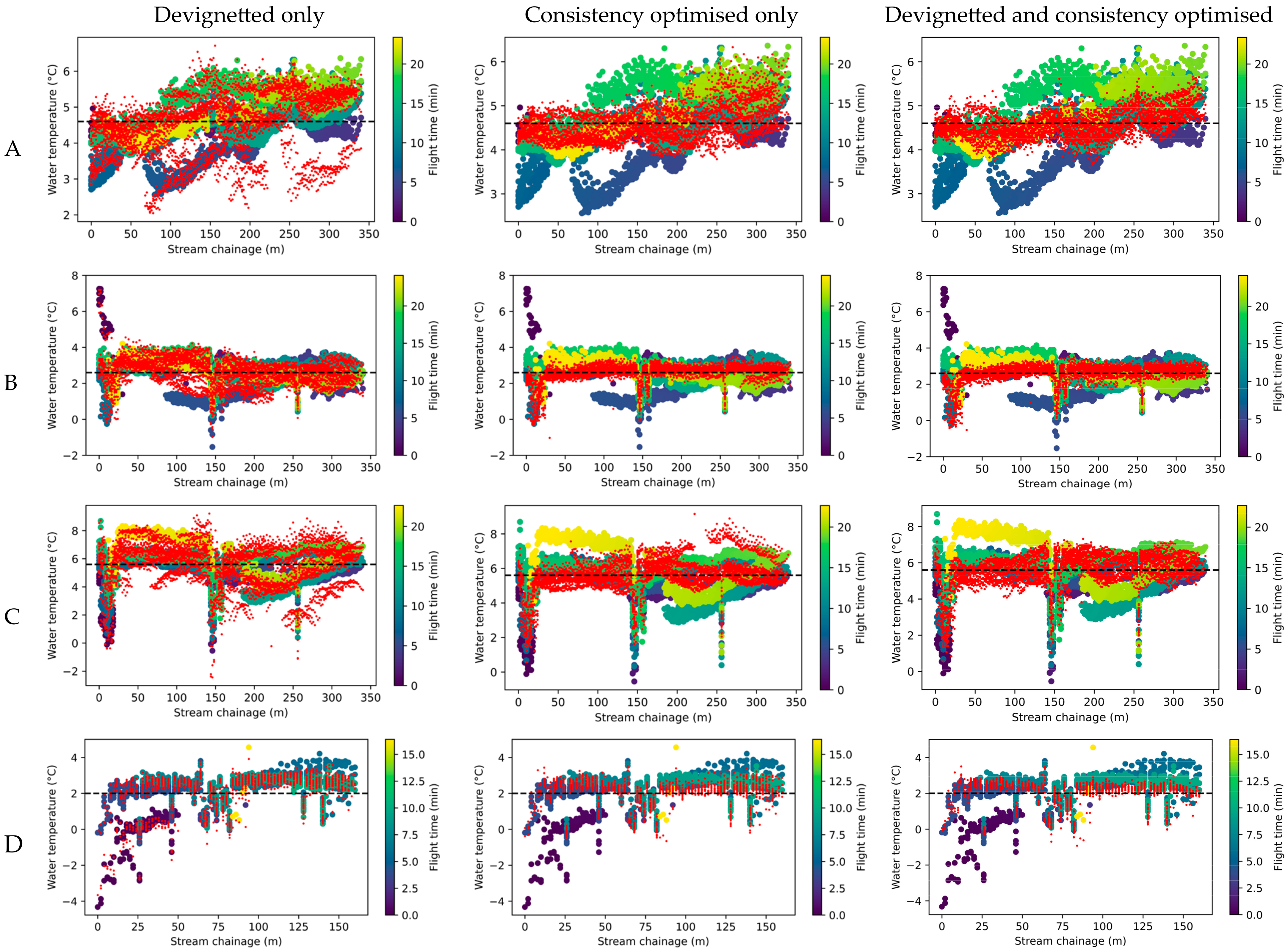
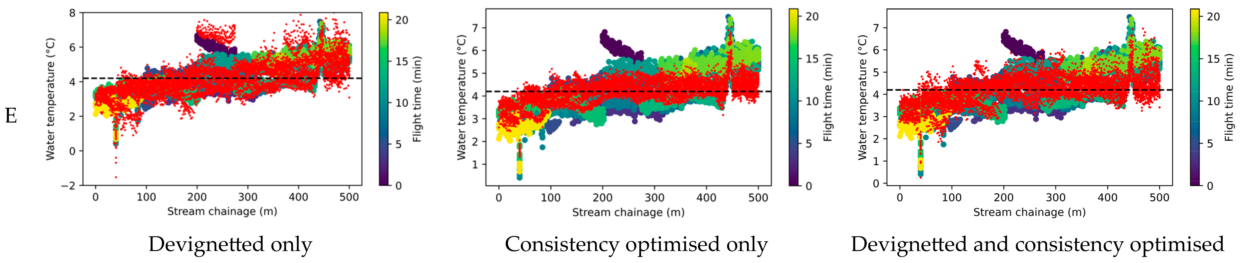
Figure 14 shows the temperature values sampled along the river centreline from the images processed using various configurations of devignetting and inter-image consistency optimisation. Since any point of the river may be present in multiple overlapping photos, several temperature readings are obtained for the same stream chainage location. The inter-image consistency optimisation procedure applied to the images from the beginning phase of the flight when the camera is warming up (dark blue markers in Figure 14) resulted in correct temperature readings in majority of the cases. The remaining outliers in the river temperature readings that have not been compensated by the algorithm, for example, three strongly negative peaks in case C in Figure 14, have proven to be sampled on vegetation overhanging the water surface.
4. Conclusions
The proposed solution significantly improved the precision of water surface temperature measurement using UAV thermal imagery. Predominant improvement came from the use of inter-image temperature consistency optimisation. Single image vignette correction had marginal impact on the final results. Calibration eliminated the clearly visible bias of images taken during the initial stage of flight that was due to warming up of the camera. This approach renders pre-flight warm-up of the camera unnecessary.
Previous methods of reducing adverse phenomena occurring in uncooled thermal cameras have relied on calibration under controlled laboratory conditions and required non-standard instrumentation such as reference black bodies or custom UAV attachments. For this reason, they require the additional effort of a specialised operator and cannot be automated. The proposed precision enhancement algorithm in opposition to those methods requires minimal effort as it only involves the data collected during a standard UAV flight and is highly automated, making it possible to use by a non-specialised operator. This also makes the solution ready to be implemented as part of a photogrammetric software workflow.
The presented method was successfully tested in the specific landscape of small river valleys in rural and suburban areas where semi-natural and anthropogenic land covers are intertwined with surface water areas with heterogeneous surface temperatures. A reliable mapping of land surface and water temperatures in such settings is important for the understanding of groundwater–surface water interactions and other physical processes that affect riverine ecosystems.
Author Contributions
Conceptualization, R.S., M.Z. and P.W.; methodology, R.S.; field work, R.S., M.Z. and P.W.; software, R.S.; validation, R.S. and A.J.-K.; formal analysis, R.S.; investigation, R.S. and A.J.-K.; resources, M.Z., P.W. and R.S.; data curation, R.S. and M.Z.; writing—original draft preparation, R.S.; writing—review and editing, P.W., M.Z. and A.J.-K.; visualization, R.S.; supervision, P.W. and M.Z.; project administration, P.W. and M.Z.; funding acquisition, P.W. and M.Z. All authors have read and agreed to the published version of the manuscript.
Funding
Research was partially funded by the National Science Centre, Poland, project WATERLINE (2020/02/Y/ST10/00065), under the CHISTERA IV programme of the EU Horizon 2020 (grant No. 857925) and the “Excellence Initiative—Research University” program at the AGH University of Krakow.
Data Availability Statement
The data presented in this study are openly available in the Zenodo repository at https://doi.org/10.5281/zenodo.8359964 (accessed on 29 September 2023). The Python implementation source code is available in the form of Jupyter notebooks at the GitHub repository https://github.com/radekszostak/aerial-thermal-tuner (accessed on 29 September 2023). Notes on implementation are included in Appendix A.
Acknowledgments
We gratefully acknowledge Poland‘s high-performance Infrastructure PLGrid (HPC Centers: ACK Cyfronet AGH, PCSS, CI TASK, WCSS) for providing computer facilities and support within computational grant no. PLG/2023/016162.
Conflicts of Interest
The authors declare no conflict of interest.
Appendix A
The algorithm was implemented in Jupyter Notebooks using the Python programming language. The processing solution includes five notebooks responsible for preliminary image conversion, vignette correction, georeferencing of images, inter-image temperature consistency optimisation, and offsetting of all images (1_conversion.ipynb, 2_devignetting.ipynb, 3_georeferencing.ipynb, 4_calibration.ipynb, respectively). They can be run on any operating system thanks to the Docker containerisation.
Appendix A.1. Conversion Notebook
First, the images must be converted from the camera manufacturer’s specific format (usually a JPG image with RGB channels providing temperature visualisation) to a single-channel TIFF file containing temperature values. For this study, the DJI thermal SDK (https://www.dji.com/pl/downloads/softwares/dji-thermal-sdk, accessed on 29 September 2023) library provided by the thermal camera manufacturer was used for the extraction of temperature arrays from manufacturer-specific JPG file format. This library requires values of flight altitude, air humidity, surface emissivity, and surface reflection temperature. The extracted temperatures are saved to a TIF file. The EXIF data is copied unchanged from the input JPG file to the resulting TIF file.
Appendix A.2. Georeferencing Notebook
For initial georeferencing, longitude (), latitude (), altitude (), and rotation () data were extracted from the images using the exiftool software. The camera’s diagonal angle of view () was taken from the camera documentation. The length of the image footprint diagonal () expressed in meters was calculated with the formula. The horizontal and vertical footprint lengths were calculated using the and formulas, respectively, where and are the width and height of the image expressed in number of pixels (in this case study, and ). The longitude and altitude were converted into , coordinates of the UTM system using the pyproj library. These are the coordinates of the centroid of the footprint of the photo. Footprint was initialized using the Polygon object of the shapely library with four corner points: , , , . It was then rotated by around the centroid using the affinity.rotate function from the shapely library to obtain the final footprint.
The rows of the matrix in the computer solutions are counted from top to bottom. It causes the vertical axis of the image reference system to point downward in the implementation. This requires modification of the transformation matrix (Equation (1)) into Equation (A1). The modified transformation matrix is similar to the standard transformation matrix with clockwise rotation; however, it uses clockwise rotation and the bottom-right pixel coordinates are used as and parameters. The modified version of the transformation matrix used in the implementation of the algorithm is presented in Equation (A1):
The modified transformation matrix was composed with and parameters being the coordinates of the bottom-right footprint corner, and parameters being the pixel sizes calculated with , parameter equal to the negative yaw value extracted from the EXIF data (as counterclockwise rotation is needed), and shear and parameters equal to zero.
In order to optimise the process of finding matches of overlapping pairs of photos, candidates are found that are potentially overlapping. The process of finding candidates consists of dilating all footprints by 5 m and then finding pairs of overlapping dilated footprints. Dilation is necessary, because due to inaccurate initial georeferencing, some of the footprints may indicate no overlap even if corresponding photos contain a common area. Then, with the help of the cv2 library, an attempt is made to stitch a given image with each of the potential neighbours. The stitching procedure consists of several steps using functions from the cv2 library: (i) detecting features and computing descriptors with the SIFT algorithm using the detectAndCompute function, (ii) descriptor matching using the knnMatch function from the FlannBasedMatcher class object, (iii) filtering out incorrect matches using the Lowe’s ratio test with a ratio value equal to , (iv) using correct matches with the estimateAffinePartial2D function to estimate the relative transformation matrix between the given image and the potential overlapping neighbour. If the number of matching points used for calculation of the transformation matrix is greater than or equal to eight, the pair of images and their relative transformation matrix are qualified for further processing. At this stage, using a relative transformation matrix, the coordinates of the corners of the stitched image in the relative reference system of the other image of the pair are also calculated.
To further ensure that the stitched pairs are correct, we filter out pairs where the scaling factor in the relative transformation matrix is outside the range of 0.8 to 1.2, as we assume that the images were taken from the same altitude, so the relative scaling factor must be equal to one.
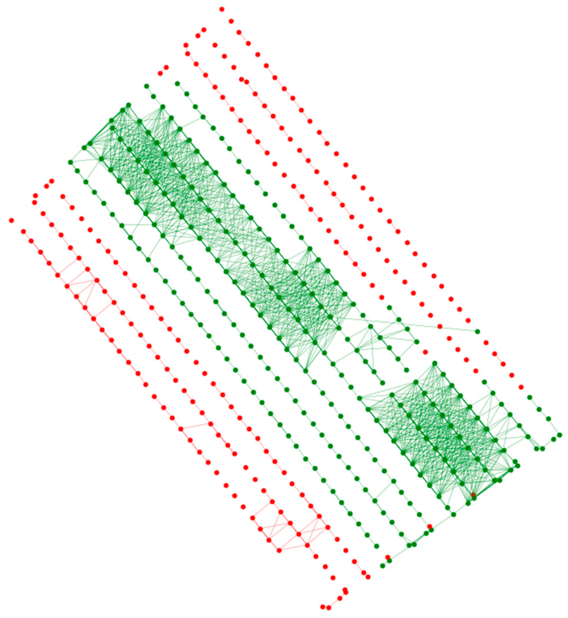
All stitched pairs of images that remain up to this point are interpreted as undirected graphs using the networkx library. Using the connected_components function, the connected component that contains the largest number of nodes (images) is extracted. It is also possible to visualise the stitched pairs and connected components as a graph with the geographical position of the nodes preserved. An example graph visualisation is shown in Figure A1.
Figure A1.
Graph visualization with preserved relative geographical positions of nodes and the largest connected component marked in green. Green nodes are used for georeferencing optimisation, red nodes are discarded. Example for D case study.
Figure A1.
Graph visualization with preserved relative geographical positions of nodes and the largest connected component marked in green. Green nodes are used for georeferencing optimisation, red nodes are discarded. Example for D case study.

The data prepared up to this point are loaded into the tensor objects of the pytorch library. Values of these tensors relate either to images or image pairs. Transformation parameters , , , , , , are stored in separate tensors of length equal number of images. These tensors will be tuned during the gradient descent optimisation, so they are initialized with the parameter requires_grad=True. A short optimisation time is ensured by using the ReduceLROnPlateau learning rate scheduler.
Appendix A.3. Calibration Notebook
Footprints are read from the previously generated GeoTIFF files. Then, based on them, pairs are found whose common part area is not less than the value defined as MIN_INTERCESTION_AREA. Samples that are the common part in pairs of images are scaled to a low resolution, defined as CLIP_SIZE. The dataset is loaded into the tensors, and gradient descent optimisation is performed.
References
- Berni, J.A.J.; Zarco-Tejada, P.J.; Suarez, L.; Fereres, E. Thermal and Narrowband Multispectral Remote Sensing for Vegetation Monitoring From an Unmanned Aerial Vehicle. IEEE Trans. Geosci. Remote Sens. 2009, 47, 722–738. [Google Scholar] [CrossRef]
- Yao, H.; Qin, R.; Chen, X. Unmanned Aerial Vehicle for Remote Sensing Applications—A Review. Remote Sens. 2019, 11, 1443. [Google Scholar] [CrossRef]
- Lagüela, S.; Díaz−Vilariño, L.; Roca, D.; Lorenzo, H. Aerial Thermography from Low-Cost UAV for the Generation of Thermographic Digital Terrain Models. Opto-Electron. Rev. 2015, 23, 76–82. [Google Scholar] [CrossRef]
- Messina, G.; Peña, J.M.; Vizzari, M.; Modica, G. A Comparison of UAV and Satellites Multispectral Imagery in Monitoring Onion Crop. An Application in the ‘Cipolla Rossa Di Tropea’ (Italy). Remote Sens. 2020, 12, 3424. [Google Scholar] [CrossRef]
- Dugdale, S.J. A Practitioner’s Guide to Thermal Infrared Remote Sensing of Rivers and Streams: Recent Advances, Precautions and Considerations. WIREs Water 2016, 3, 251–268. [Google Scholar] [CrossRef]
- Dugdale, S.J.; Kelleher, C.A.; Malcolm, I.A.; Caldwell, S.; Hannah, D.M. Assessing the Potential of Drone-based Thermal Infrared Imagery for Quantifying River Temperature Heterogeneity. Hydrol. Process. 2019, 33, 1152–1163. [Google Scholar] [CrossRef]
- O’Sullivan, A.M.; Linnansaari, T.; Curry, R.A. Ice Cover Exists: A Quick Method to Delineate Groundwater Inputs in Running Waters for Cold and Temperate Regions. Hydrol. Process. 2019, 33, 3297–3309. [Google Scholar] [CrossRef]
- Aragon, B.; Phinn, S.R.; Johansen, K.; Parkes, S.; Malbeteau, Y.; Al-Mashharawi, S.; Alamoudi, T.S.; Andrade, C.F.; Turner, D.; Lucieer, A.; et al. A Calibration Procedure for Field and UAV-Based Uncooled Thermal Infrared Instruments. Sensors 2020, 20, 3316. [Google Scholar] [CrossRef] [PubMed]
- Kelly, J.; Kljun, N.; Olsson, P.-O.; Mihai, L.; Liljeblad, B.; Weslien, P.; Klemedtsson, L.; Eklundh, L. Challenges and Best Practices for Deriving Temperature Data from an Uncalibrated UAV Thermal Infrared Camera. Remote Sens. 2019, 11, 567. [Google Scholar] [CrossRef]
- Kusnierek, K.; Korsaeth, A. Challenges in Using an Analog Uncooled Microbolometer Thermal Camera to Measure Crop Temperature. Int. J. Agric. Biol. Eng. 2014, 7, 60–74. [Google Scholar]
- Yuan, W.; Hua, W. A Case Study of Vignetting Nonuniformity in UAV-Based Uncooled Thermal Cameras. Drones 2022, 6, 394. [Google Scholar] [CrossRef]
- Ribeiro-Gomes, K.; Hernández-López, D.; Ortega, J.; Ballesteros, R.; Poblete, T.; Moreno, M. Uncooled Thermal Camera Calibration and Optimization of the Photogrammetry Process for UAV Applications in Agriculture. Sensors 2017, 17, 2173. [Google Scholar] [CrossRef] [PubMed]
- Lin, D.; Maas, H.-G.; Westfeld, P.; Budzier, H.; Gerlach, G. An Advanced Radiometric Calibration Approach for Uncooled Thermal Cameras. Photogramm. Rec. 2018, 33, 30–48. [Google Scholar] [CrossRef]
- Sampath, A.; Moe, D.; Christopherson, J. Two methods for self calibration of digital camera. Int. Arch. Photogramm. Remote Sens. Spat. Inf. Sci. 2012, 39, 261–266. [Google Scholar] [CrossRef]
- Mesas-Carrascosa, F.J.; Pérez-Porras, F.J.; Larriva, J.E.M.D.; Frau, C.M.; Agüera-Vega, F.; Carvajal-Ramírez, F.; Martínez-Carricondo, P.; García-Ferrer, A. Drift Correction of Lightweight Microbolometer Thermal Sensors On-Board Unmanned Aerial Vehicles. Remote Sens. 2018, 10, 615. [Google Scholar] [CrossRef]
- Kingma, D.P.; Ba, J. Adam: A Method for Stochastic Optimization. arXiv 2014, arXiv:1412.6980. [Google Scholar] [CrossRef]
- Sedano-Cibrián, J.; Pérez-Álvarez, R.; De Luis-Ruiz, J.M.; Pereda-García, R.; Salas-Menocal, B.R. Thermal Water Prospection with UAV, Low-Cost Sensors and GIS. Application to the Case of La Hermida. Sensors 2022, 22, 6756. [Google Scholar] [CrossRef] [PubMed]
- Zheng, Y.; Lin, S.; Kambhamettu, C.; Yu, J.; Kang, S.B. Single-Image Vignetting Correction. IEEE Trans. Pattern Anal. Mach. Intell. 2009, 31, 2243–2256. [Google Scholar] [CrossRef] [PubMed]
- Huang, L.Y. Luna983/Stitch-Aerial-Photos: Stable v1.1. 2020. Available online: https://github.com/luna983/stitch-aerial-photos (accessed on 18 June 2023).
- Lowe, D.G. Distinctive Image Features from Scale-Invariant Keypoints. Int. J. Comput. Vis. 2004, 60, 91–110. [Google Scholar] [CrossRef]
- Muja, M.; Lowe, D.G. Fast Approximate Nearest Neighbors with Automatic Algorithm Configuration. In Proceedings of the Fourth International Conference on Computer Vision Theory and Applications (VISIGRAPP 2009)—Volume 1: VISAPP, Lisboa, Portugal, 5–8 February 2009; pp. 331–340. [Google Scholar]
- Fischler, M.A.; Bolles, R.C. Random Sample Consensus: A Paradigm for Model Fitting with Applications to Image Analysis and Automated Cartography. Commun. ACM 1981, 24, 381–395. [Google Scholar] [CrossRef]
- John, C.; Allan, H.D. A First Look at Graph Theory; Allied Publishers: New Delhi, India, 1995. [Google Scholar]
Figure 1.
A block diagram of proposed self-calibration method consisting of the precision enhancement steps (solid box) and optional accuracy enhancement step (dashed box).
Figure 1.
A block diagram of proposed self-calibration method consisting of the precision enhancement steps (solid box) and optional accuracy enhancement step (dashed box).

Figure 2.
Visualisation of the alignment procedure of an example pair of images with dimensions of pixels. The coordinates of the marked corners are expressed in the pixel coordinate system of the first image.
Figure 2.
Visualisation of the alignment procedure of an example pair of images with dimensions of pixels. The coordinates of the marked corners are expressed in the pixel coordinate system of the first image.

Figure 3.
Example of cropped areas and the common area in a pair of images used for temperature adjustment.
Figure 3.
Example of cropped areas and the common area in a pair of images used for temperature adjustment.

Figure 4.
Example components of the dataset sample: (a) binary mask, (b) first temperature image, (c) second temperature image.
Figure 4.
Example components of the dataset sample: (a) binary mask, (b) first temperature image, (c) second temperature image.

Figure 5.
An example of successful devignetting: (a) top left, original image, (b) top right, the same image after applying devignetting procedure, (c) bottom, pixel temperature distributions of the original and corrected image.
Figure 5.
An example of successful devignetting: (a) top left, original image, (b) top right, the same image after applying devignetting procedure, (c) bottom, pixel temperature distributions of the original and corrected image.

Figure 6.
An example of unsuccessful devignetting: (a) top left, original image, (b) top right, the same image after applying devignetting procedure, (c) bottom, pixel temperature distributions of the original and corrected image. The river is a bright streak along the left edge of the image.
Figure 6.
An example of unsuccessful devignetting: (a) top left, original image, (b) top right, the same image after applying devignetting procedure, (c) bottom, pixel temperature distributions of the original and corrected image. The river is a bright streak along the left edge of the image.

Figure 7.
Change in the image temperature standard deviation as a result of the devignetting algorithm. Negative values imply improvement (lowering of the standard deviation in a corrected image). The dashed line is drawn at 0 °C.
Figure 7.
Change in the image temperature standard deviation as a result of the devignetting algorithm. Negative values imply improvement (lowering of the standard deviation in a corrected image). The dashed line is drawn at 0 °C.

Figure 8.
Case A—image mosaic before (left) and after (right) the calibration.

Figure 9.
Case B—image mosaic before (left) and after (right) the calibration.

Figure 10.
Case C—image mosaic before (left) and after (right) the calibration.

Figure 11.
Case D—image mosaic before (left) and after (right) the calibration.

Figure 12.
Case E—image mosaic before (left) and after (right) the calibration.

Figure 13.
Root mean square errors of waterbody temperature before calibration, after devignetting only, after consistency optimisation only, and after devignetting and consistency optimisation.
Figure 13.
Root mean square errors of waterbody temperature before calibration, after devignetting only, after consistency optimisation only, and after devignetting and consistency optimisation.

Figure 14.
Temperature values sampled along river centreline from devignetted only (left column), optimised only (middle column), and both devignetted and optimised (right column) images plotted as small red points. Large colour-scale points show the temperature sampled from unprocessed images, the colours themselves indicating time of flight in minutes. The dashed line indicates actual water temperature measured with a thermocouple. Rows A to E correspond to locations (see Table 1).


Table 1.
Details of the surveys carried out.
| Alias | Location | Time | Conditions | Water Temperature |
|---|---|---|---|---|
| A | Kocinka, Rybna | 15 December 2021 12:20 | Fog, snow cover | 4.6 °C |
| B | Kocinka, Rybna | 18 January 2022 14:55 | Snow cover, total cloud cover | 2.6 °C |
| C | Kocinka, Rybna | 25 March 2022 07:30 | No cloud cover | 5.6 °C |
| D | Sudół, Kraków | 20 December 2022 11:20 | Moderate cloud cover | 2.0 °C |
| E | Kocinka, Grodzisko | 11 January 2023 11:00 | No cloud cover | 4.2 °C |
Disclaimer/Publisher’s Note: The statements, opinions and data contained in all publications are solely those of the individual author(s) and contributor(s) and not of MDPI and/or the editor(s). MDPI and/or the editor(s) disclaim responsibility for any injury to people or property resulting from any ideas, methods, instructions or products referred to in the content. |
© 2023 by the authors. Licensee MDPI, Basel, Switzerland. This article is an open access article distributed under the terms and conditions of the Creative Commons Attribution (CC BY) license (https://creativecommons.org/licenses/by/4.0/).
Share and Cite
MDPI and ACS Style
Szostak, R.; Zimnoch, M.; Wachniew, P.; Jasek-Kamińska, A. Self-Calibration of UAV Thermal Imagery Using Gradient Descent Algorithm. Drones 2023, 7, 683. https://doi.org/10.3390/drones7110683
AMA Style
Szostak R, Zimnoch M, Wachniew P, Jasek-Kamińska A. Self-Calibration of UAV Thermal Imagery Using Gradient Descent Algorithm. Drones. 2023; 7(11):683. https://doi.org/10.3390/drones7110683
Chicago/Turabian StyleSzostak, Radosław, Mirosław Zimnoch, Przemysław Wachniew, and Alina Jasek-Kamińska. 2023. "Self-Calibration of UAV Thermal Imagery Using Gradient Descent Algorithm" Drones 7, no. 11: 683. https://doi.org/10.3390/drones7110683